Time optimal information transfer in spintronics networks

Abstract

Propagation of information encoded in spin degrees of freedom through networks of coupled spins enables important applications in spintronics and quantum information processing. We study control of information propagation in networks of spin-$\tfrac{1}{2}$ particles with uniform nearest neighbor couplings forming a ring with a single excitation in the network as simple prototype of a router for spin-based information. Specifically optimizing spatially distributed potentials, which remain constant during information transfer, simplifies the implementation of the routing scheme. However, the limited degrees of freedom makes finding a control that maximizes the transfer probability in a short time difficult. We show that the structure of the eigenvalues and eigenvectors must fulfill a specific condition to be able to maximize the transfer fidelity, and demonstrate that a specific choice among the many potential structures that fulfill this condition significantly improves the solutions found by optimal control.

I INTRODUCTION

Encoding information spin degrees of freedom has the potential to revolutionize information technology via the development of novel spintronic devices and possible future quantum information processors [1, 2]. Utilizing information encoded in spin degrees of freedom, however, requires efficient, controlled on-chip transfer of spin-based information. In some types of spintronic devices, spin degrees of freedom are used in addition to motional degrees of freedom of electrons, and information encoded in the spin degrees of freedom can be transferred using conventional currents. In principle, however, information stored in spin states can propagate through a network of coupled spins without charge transport. As propagation of spin-based information is governed by quantum-mechanics and the Schrödinger equation, however, excitations in a spin network propagate, disperse and refocus in a wave-like manner, and controlling information transport is thus a quantum control problem. Without any means to control the propagation of spin-based information in such networks information transport can be slow and inefficient. Control can be utilized to optimize transport in terms of maximizing transfer efficiency and speed [3, 4]. Here, we consider how to control information propagation in a network of spins by optimizing spatially distributed potentials, which remain constant during the evolution, in contrast to dynamic control schemes, which require dynamic modulation or fast switching of the control potentials.

II THEORY AND METHODS

II-A Networks of coupled spins

We restrict ourselves to spin-$\tfrac{1}{2}$ particles with two spin states labeled $|0\rangle$ and $|1\rangle$ as a simple prototype device for routing spin-based information. The energies of the spin states of spin $n$ differ by small amounts $\Delta_{n}$. Nearby spins can interact, e.g., by exchange coupling. This leads to a model Hamiltonian for a network of coupled spins of the form

$$H_{\rm full}=\sum_{n=1}^{N}\Delta_{n}Z_{n}+\sum_{m\neq n}J_{mn}[X_{m}X_{n}+Y_{m}Y_{n}+\kappa Z_{m}Z_{n}],$$ (1)

where $\kappa$ is a parameter depending on the type of coupling, e.g., $\kappa=1$ for isotropic Heisenberg coupling and $\kappa=0$ for pure $XX$ coupling. $X_{n}$, $Y_{n}$ and $Z_{n}$ are operators acting on the $2^{N}$ dimensional Hilbert space of the $N$-spin network. $X_{n}$ is a tensor product of $N-1$ identity operators with a single $X$ operator in the $n$th position, and similarly for $Y_{n}$ and $Z_{n}$. $X$, $Y$ and $Z$ are the Pauli spin operators

$$X=\begin{pmatrix}0&1\\ 1&0\end{pmatrix},\quad Y=\begin{pmatrix}0&-i\\ i&0\end{pmatrix},\quad Z=\begin{pmatrix}1&0\\ 0&-1\end{pmatrix}.$$ (2)

For networks with uniform coupling all non-zero couplings have the same strength $J$ and we can set $J=1$ by choosing the frequencies in units of $J$ and time in units of $J^{-1}$.

It can be easily verified that a Hamiltonian of the form (1) commutes with the total excitation operator $\sum_{n}Z_{n}$. The Hilbert space of the system therefore decomposes into excitation subspaces [6]. If we assume that only a single excitation (or bit of information) propagates through the network at any given time, then the Hamiltonian can be reduced to the single excitation subspace Hamiltonian

$$H=\Delta_{n}|n\rangle\langle n|+J_{mn}|m\rangle\langle n|,$$ (3)

where $|m\rangle\langle n|$ can be thought of as a matrix which is zero except for a $1$ in the $(m,n)$ position. Which $J_{mn}$ are non-zero depends on the network topology. For a chain with nearest-neighbor coupling we have $J_{mn}=0$ unless $m=n\pm 1$, and similarly for a ring arrangement, except that for the latter we also have $J_{N,1}=J_{1,N}\neq 0$. While a linear chain can be thought of as a type of quantum wire, a ring can be regarded as a basic routing element to distribute spin states, e.g., to chains attached to various nodes of the ring (see Fig. 1).

II-B Dynamic vs static control

Dynamic control involves dynamically altering certain couplings $J_{mn}$ or potentials $\Delta_{n}$. This is a powerful tool and has been explored in previous work [5]. However, it typically requires the ability to rapidly modulate or switch fields. Furthermore, for networks with a high degree of symmetry such as rings with uniform coupling, controllability is generally limited by dynamic symmetries [6]. An alternative to this dynamic control is to shape the potential landscape to facilitate the flow of information from an initial state (input node) to a target state (output node). For example, for information encoded in nuclear spins or electron spins in quantum dots whose potential can be controlled by surface control electrodes, this could be achieved by varying the voltages to create a potential landscape as shown in Fig. 1.

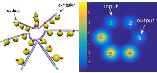
Figure 1: Spin network ring extended with chains (left) and potential landscape created by local biases optimized for information transfer from node 1 to 3 in a 6 ring (right).

Fixing the network topology defined by the couplings $J_{mn}$ and applying potentials $\Delta_{n}$ that are constant in time, gives the constant Hamiltonian $H_{\Delta}=H_{0}+\mbox{diag}(\Delta_{n})$ and the information transfer is governed by the Schrödinger equation

$$i\hbar\dot{U}(t)=H_{\Delta}U(t),\quad U(0)=I,$$ (4)

where $U(t)$ is a unitary propagation operator, initially equal to the identity operator $I$. The probability of transmission of information from the input node $|\mathrm{in}\rangle$ to the output node $|\mathrm{out}\rangle$ in time $t$ is then given by

$$p(t)=|\langle\mathrm{out}|e^{-itH_{\Delta}}|\mathrm{in}\rangle|^{2}.$$ (5)

Assuming the energies $\Delta_{n}$ are controllable, we have a vector of control parameters $\Delta=(\Delta_{n})$ and the objective is to find a $\Delta$ such that

$$p(t)=\max_{\Delta}|\langle\mathrm{out}|e^{-itH_{\Delta}}|\mathrm{in}\rangle|^{2}$$ (6)

at some time $t$. We can fix the time $t=t_{f}$, require that $t\leq t_{\max}$ where $t_{\max}$ is an upper bound, or attempt to accomplish the transfer with maximum fidelity in minimum time. These problems can in principle be solved in a straightforward manner using standard optimization tools although the optimization landscape is challenging, in particular when the goal is to find a control that achieves the highest possible fidelity in the shortest time possible as this effectively creates two objectives for the optimization.

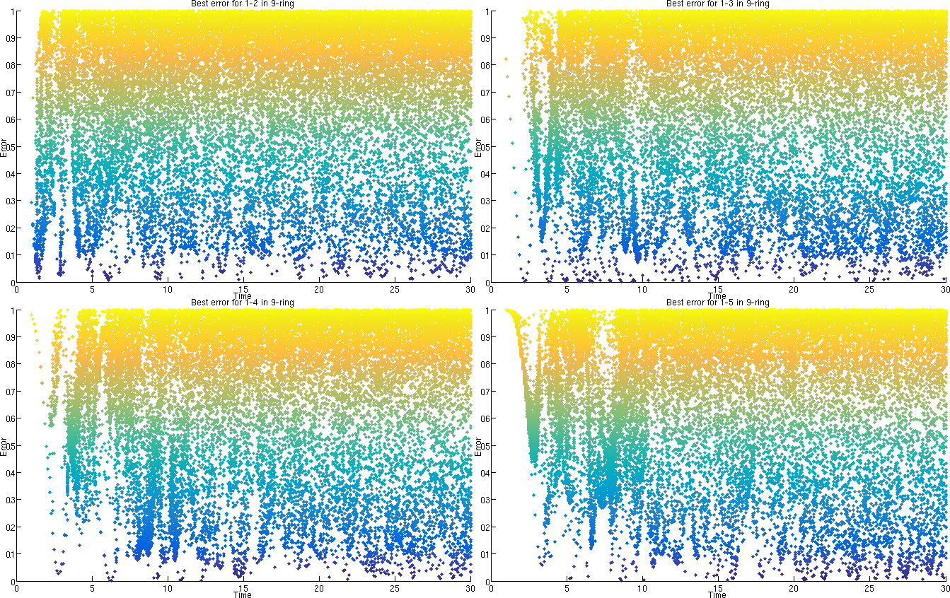
Figure 2: Results of optimizing the information propagation from spin $1$ to $2$ (top left), $3$ (top right), $4$ (bottom left) and $5$ (bottom right) for a ring of $9$ spins using a quasi-Newton L-BFGS optimization with exact gradient on static biases for fixed times $f_{f}$ from $1$ to $30$ with step size $0.2$. Each data point represents the infidelity $1-p(t)$ achieved for the corresponding time, indicating that the optimization gets trapped often, even if many repeats can still find good solutions for certain times.

II-C Eigenstructure optimization

We can reformulate the control problem by diagonalizing the Hamiltonian, $H_{\Delta}=V\Lambda V^{\dagger}$, where $V$ is a unitary matrix of the eigenvectors and $\Lambda$ a diagonal matrix of the eigenvalues of $H_{\Delta}$. Then $U=e^{-itH_{\Delta}}=VEV^{\dagger}$ with $E=\mbox{diag}(e^{-i\lambda_{n}t})$ and our control objective is to ensure

$$V^{\dagger}|\mathrm{out}\rangle=e^{i\phi}EV^{\dagger}|\mathrm{in}\rangle,$$ (7)

where $\phi$ is a global phase factor, which we introduce to cancel the the global phase of the output state.

For a network with ring topology, we can take the input state to be $|1\rangle=(1,0,\ldots)^{T}$ due to translation invariance, and the output state to be $|k\rangle$, $k\leq\lceil N/2\rceil$. Then Eq. (7) becomes

$$v_{n,k}^{*}=e^{-i(t\lambda_{n}-\phi)}v_{n,1}^{*},\quad\forall n=1,\ldots,N.$$ (8)

Thus, the optimization problem is equivalent to finding the a control vector $\Delta$ and phase $\phi$ that minimize

$$\sum_{n}|v_{k,n}-e^{i(t\lambda_{n}-\phi)}v_{1,n}|^{2}$$ (9)

Note that only the $1$st and $k$th component of the eigenvectors (or $1$st and $k$th rows of $V$) and eigenvalues $\lambda_{n}$ matter.

The upper bound on the fidelity of the transmission given no time constraints, referred to as Information Transfer Fidelity [8, 9], is given by

$$\sqrt{\mathrm{ITF}}=\sum_{n=1}^{N}|\langle\mathrm{in}|v_{n}\rangle\langle v_{n}|\mathrm{out}\rangle|=\sum_{n=1}^{N}s_{n}\langle\mathrm{in}|v_{n}\rangle\langle v_{n}|\mathrm{out}\rangle,$$ (10)

where $s_{n}=\mathrm{sign}(\langle\mathrm{in}|v_{n}\rangle\langle v_{n}|\mathrm{out}\rangle)$. Since it is a probability, $\mathrm{ITF}\leq 1$. Here we use some eigenstructure assignment concept [7] to show that, given $|\mathrm{in}\rangle$ and $|\mathrm{out}\rangle$, there always exists an orthonormal reference frame $\{v_{n}:n=1,...,N\}$ such that the upper bound $\mathrm{ITF}\leq 1$ is achieved. The issue as to whether this reference frame can be achieved by an optimal biasing strategy $\Delta=(\Delta_{n})_{n=1}^{N}$ is open, but numerical exploration seems to indicate that the optimal biases in the sense of Sec. III reproduce this frame with high accuracy.

Instead of deriving the position of the reference frame $\{v_{k}:k=1,...,N\}$ relative to the input and output states, we reformulate the problem as the one of finding the position of the input and output states relative to a given (orthonormal) reference frame $\{v_{n}:n=1,...,N\}$. Let $\langle v_{n}|\mathrm{in}\rangle$, $\langle v_{n}|\mathrm{out}\rangle$, $n=1,...,N$, be the coordinates of the input and output states, resp., in the reference frame $\{v_{k}:k=1,...,N\}$. The problem is to maximize Eq. (10) subject to the constraints

$$\langle\mathrm{out}|\mathrm{in}\rangle=0,\quad\langle\mathrm{in}|\mathrm{in}\rangle=1,\quad\langle\mathrm{out}|\mathrm{out}\rangle=1.$$

Define the Lagrange multipliers $\lambda$, $\mu$, $\kappa$ and the augmented functional

$$\sum_{n=1}^{N}s_{n}\langle v_{n}|\mathrm{in}\rangle^{*}\langle v_{n}|\mathrm{out}\rangle+\lambda\langle\mathrm{out}|\mathrm{in}\rangle+\tfrac{\kappa}{2}\langle\mathrm{in}|\mathrm{in}\rangle+\tfrac{\mu}{2}\langle\mathrm{out}|\mathrm{out}\rangle$$

The classical first order condition for optimality yields

$$\begin{pmatrix}\lambda+s_{n}&\mu\\ \kappa&\lambda+s_{n}\end{pmatrix}\begin{pmatrix}\langle v_{n}|\mathrm{in}\rangle\\ \langle v_{n}|\mathrm{out}\rangle\end{pmatrix}=0,\quad n=1,...,N.$$ (11)

Existence of a solution yields

$$\lambda=(\pm)\sqrt{\kappa\mu}-s_{n}.$$

The crucial issue is to observe that $\lambda$ should be independent of $n$. At optimality, not all $s_{n}$’s could be of the same sign (otherwise $\mathrm{ITF}=|\langle\mathrm{out}|\mathrm{in}\rangle|^{2}=0$). This implies that $s_{n}=(\pm)$ and $\sqrt{\kappa\mu}=1$. From there on, solving (11), and after some manipulation, it is found that

$$\langle v_{n}|\mathrm{in}\rangle=\pm\langle v_{n}|\mathrm{out}\rangle,\quad n=1,\ldots,N.$$

As already said, the optimal biases $\Delta_{n}$’s appear to reproduce this result. The above eigenvector assignment is non-unique and dimension dependent. When $N=2$, the solution is already far from unique. Up to permutation, either $\{|\mathrm{in}\rangle,|\mathrm{out}\rangle\}$ is in $\mathrm{span}\{v_{1},v_{2}\}$ and offset at a $45^{\circ}$ angle or $|\mathrm{in}\rangle=(1/\sqrt{4})(1,1,1,1)$ and $|\mathrm{out}\rangle=1/\sqrt{4}(1,-1,1,-1)$.

III RESULTS

III-A General optimization results

Solving the optimization problem given by Eq. (6) directly for a fixed target time $t_{f}$ is challenging even without constraints on the biases $\Delta$ as the landscape is extremely complicated with many local extrema, resulting in trapping of local optimization approaches such as quasi-Newton methods. Fig. 2 shows the results of various runs for fixed times for a ring of $9$ spins, with the objective being to propagate the excitation from spin $1$ to spin $2$, $3$, $4$ and $5$, respectively. Fixed time values $t_{f}$ from $1$ to $30$ with steps of $0.2$ were set and a quasi-Newton optimizer with random initial values for the biases repeated $100$ times for each $t_{f}$. Each point in this plot represents one run for the respective time $t_{f}$ and the achieved infidelity value $1-p(t)$. There are many points for which the error is large (i.e., the transmission fidelity is low), indicating that the optimization for this run converged to a local extremum, making finding a good solution very expensive. We also tested some global search algorithms that appeared successful for hard optimization problems such as a variant of differential evolution used in [10], but these proved to be much slower and produced generally worse results than the best solutions found by repeating a quasi-Newton optimization algorithm for a relatively large number of initial states. The results in Fig. 2 also indicate that there are only certain times for which we can expect to find a high information transfer fidelity.

Instead of fixing the time we can also add the time as additional parameter to optimize over and start for random initial biases and times. The results of this are shown in Fig. 3 for the propagation from spin $1$ to $5$ in a ring of $13$ spins. We report the solution with the highest fidelity overall and the fastest solution with a fidelity larger than $0.99$. Typically the highest fidelity solutions are found at longer times but good solutions for short times are also achieved. However, many restarts of the optimization are required, and many runs fail with fidelities smaller than $0.9$. Inspection of the good solutions found showed that many of these involved biases that were highly mirror symmetric w.r.t. the symmetry axis between the input and output spin on the ring.

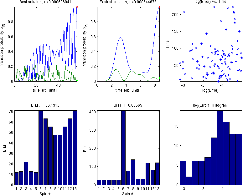
Figure 3: Results for optimizing the information transfer probability from spin $1$ to $5$ for a ring of $13$ spins over the spatial biases and times starting from random initial biases and times. Left-bottom shows the biases giving the best fidelity at time $T\approx 56.19$ yielding the $p(t)$ shown in the left-top image (in blue vs. the natural evolution in green). The two graphs in the middle show the fastest solution found with a fidelity greater than $0.99$ at time $T\approx 8.63$. Right-top shows the overall found solutions by the optimization plotting the time vs. the logarithm of the infidelity. Right-bottom plots a histogram of the logarithm of the infidelity.

III-B Finding good initial values

In principle the information transfer fidelity depends on all eigenvectors and eigenvalues of the Hamiltonian. However, the results in Section II-C show that the structure of the eigenvalues and eigenvectors must fulfill a specific condition to be able to maximize the transfer fidelity. While there are many potential structures that fulfill the condition, we can choose a specific one to provide a guide for good initial values or a restricted domain for the population. This significantly improved the solutions found by the optimal control algorithms.

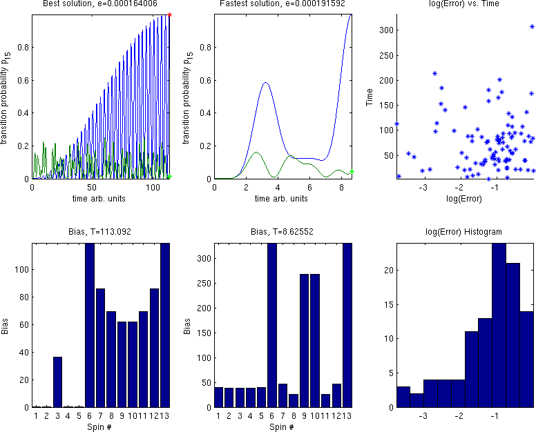
Figure 4: Results for optimizing the information transfer probability from spin $1$ to $5$ for a ring of $13$ spins over the spatial biases and times starting from random initial biases and times, where the biases are constrained to be symmetric across the axis going through the middle between initial and target state. Left-bottom shows the biases giving the best fidelity at time $T\approx 113.09$ yielding the $p(t)$ shown in the left-top image (in blue vs. the natural evolution in green). The two graphs in the middle show the fastest solution found with a fidelity greater than $0.99$ at time $T\approx 8.63$. Right-top shows the overall found solutions by the optimization plotting the time vs. the logarithm of the infidelity. Right-bottom plots a histogram of the logarithm of the infidelity.

The basic idea for imposing a specific eigenstructure is to quench the ring of $N$ spins into a chain from the initial spin to the target spin. Our previous work showed that this can be easily achieved by applying a very strong potential in the middle between the initial and target spin [3]. If we can control the potentials of all spins then we can generalize this to quench the ring just before the initial and after the target node, giving two options for a chain connecting the two nodes where either could provide a solution. As it turns out, this gives rise to a general eigenstructure induced by applying mirror symmetric potentials across the axis going through the middle between initial and target state in the ring. We consequently choose such symmetric potentials in combination with the approximate times where the maximum fidelity is achieved in the related chains as initial values for the optimal control algorithm. This significantly improves the results and efficiently finds controls for maximum information transfer in minimum time for any initial and target spin. This approach is also further justified by the results found using random initial values.

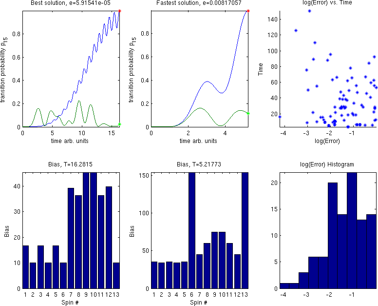
Figure 5: Results for information transfer from spin $1$ to $5$ in a ring of $13$ spins, optimizing both spatial biases and transfer times, starting with initial times corresponding to peaks in the chain transition and random biases. Left-bottom shows the biases giving the best fidelity at time $T\approx 16.28$ yielding the $p(t)$ in left-top graph (in blue vs. the natural evolution in green). The graphs in the middle show the fastest solution found with a fidelity greater than $0.99$ at time $T\approx 5.22$. Top-right plot shows the time-error distribution of the solutions found over $100$ runs and bottom right graphs shows a histogram of the logarithmic infidelity.

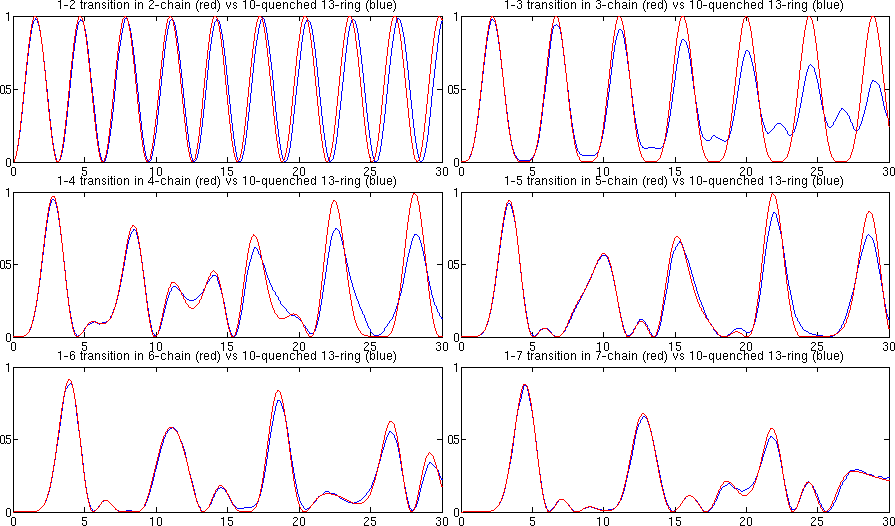
Figure 6: Information transfer probabilities for $1$ to $k=2,3,4,5,6,7$ in $13$-ring (blue) with a bias of $10$ on the spins from $k+1$ to $13$ vs. end-to-end natural transfer in $k$ chain (red)

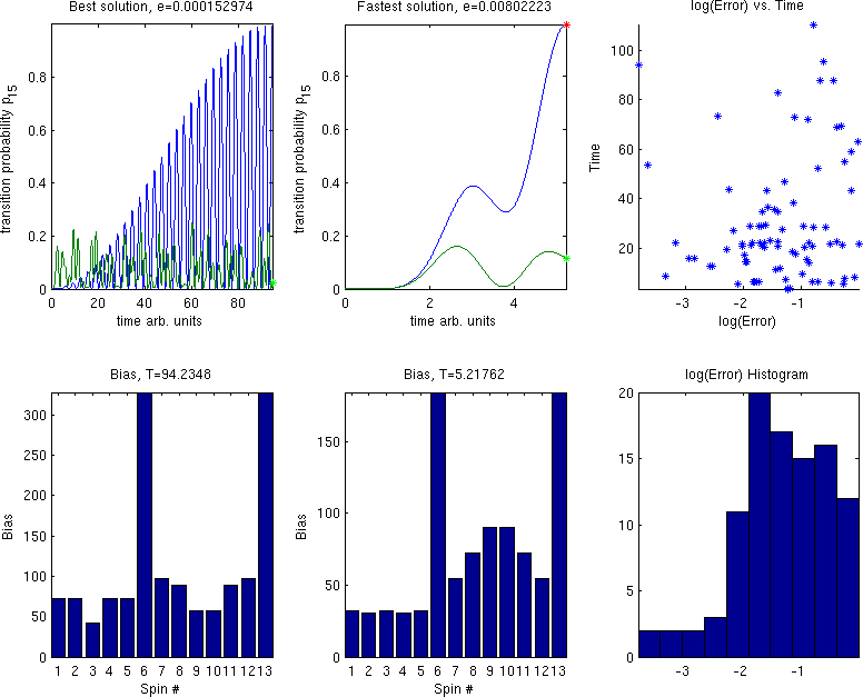
Figure 7: Results for information transfer from spin $1$ to $5$ for a ring of $13$ spins, optimizing both transfer times and spatial biases, starting with initial times derived from the peaks of the corresponding chain transition and biases that are random but subject to symmetry constraints. Left-bottom shows the biases giving the best fidelity at time $T\approx 94.23$ yielding the $p(t)$ shown in the left-top image (in blue vs. the natural evolution in green). Middle graphs show the fastest solution found with a fidelity greater than $0.99$ at time $T\approx 5.22$. Right-top shows the overall found solutions by the optimization plotting the time vs. the logarithm of the infidelity. Right-bottom plot shows histogram of logarithmic infidelity.

The symmetry constraint can be easily applied by reducing the number of biases to be found to $\lceil N/2\rceil$, symmetric across the symmetry axis between initial and target state. Fig. 4 shows the results with this constraint similar to the results in Fig. 3 without the symmetry constraint. Similar shortest time solutions are found, while the best solution is at a different time. This is not surprising considering that the solution found strongly depends on initial values. More importantly, there are slightly fewer failed runs. Convergence of the optimization can be further improved by selecting constants, peaks or troughs as biases between initial and target spin on both sides of the ring randomly.

Fig. 6 compares the information transfer probabilities from spin $1$ to $k$ in an $N$ ring with a constant bias on the spins $k$ to $N$ with the information transfer probabilities between the end nodes of a chain of length $k$. From this example and theory [3] it is obvious that the maxima coincide and the stronger the bias the more similar the information transfer probabilities between the quenched ring and the chain. Hence, it seems likely that we can obtain better results if the initial times are taken from the largest peaks, say those over $0.8$, of the chain transition, which can easily be approximated by evaluating the probabilities for the chain at a regular sampling.

Fig. 5 shows the results for the $1$ to $5$ transition of the $13$ ring for random, unconstrained initial biases and the initial times taken from the peaks of the corresponding $1$ to $5$ transition in a $5$ chain. This resulted in a faster time being found, but still quite a few failed runs. Combining this with the symmetry constraint gives the results shown in Fig. 7, resulting in the same short time and fewer failed runs.

We can further add a constraint to limit the strength of the biases. Fig. 8 shows the results. To achieve the same effect of quenching the ring to a chain, all potentials are moved towards the maximum instead of pushing the two potentials at the two end spins to very high values.

Overall, results for other rings and transitions are similar to the results presented for the $1$ to $5$ transition for a ring of size $N=13$. Fig 9 shows the shortest times achieved for transition fidelities greater than $0.99$. This indicates that the shortest transition times depend largely on the distance between the spins and not the size of the ring, consistent with quenching the ring into a chain. Although we have no proof that there is no shorter transition time, the results seem to indicate that the shortest time in the ring is closely related to the time of the natural evolution to the corresponding chain, in case of static bias controls.

In special cases we can further derive values for the expected minimum transfer time and the corresponding biases. If the distance between the initial and target spin is $1$ then quenching the ring as described reduces the network to a two-spin system with direct coupling and an effective Hamiltonian of the form $H=\begin{pmatrix}c_{1}&1\\ 1&c_{2}\end{pmatrix}$ which undergoes Rabi oscillations with the Rabi frequency $\Omega=\sqrt{(c_{2}-c_{1})^{2}+4}$. It can easily be shown that $p_{12}(t)=(\tfrac{1}{2}\Omega)^{-2}\sin^{2}(\tfrac{1}{2}{\Omega}t)$. The maximum $p_{12}=1$ is assumed for $t=\tfrac{\pi}{2}$, if and only if $\Omega=2$, or $c_{1}=c_{2}$. Indeed the numerical optimization results in Fig. 2 for transfer from $1$ to $2$ (top left) in a ring of size $9$ show that the first minimum is close to $0$ and occurs for $t\approx\pi/2$.

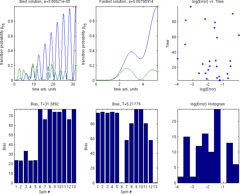
Figure 8: Results for information transfer from spin $1$ to $5$ in a ring of $13$ spins, optimizing both spatial biases and transfer times, starting with initial times corresponding to peaks in the chain transition and biases that are random but subject to symmetry and amplitude constraints $0\leq\Delta_{n}\leq 100$. Left-bottom shows biases giving the best fidelity at time $T\approx 94.23$ yielding $p(t)$ shown in the left-top image (in blue vs. natural evolution in green). The graphs in the middle show the fastest solution found with a fidelity $>0.99$ at time $T\approx 5.22$. Top-right plot shows the time-error distribution of the solutions found over $100$ runs and bottom right graphs shows a histogram of the logarithmic infidelity.

Similarly, if the distance is $2$ the ring is reduced to a three-spin chain. In this case we can easily show that, assuming zero-bias, $\Delta=(0,0,0)$, $p_{13}=\sin^{4}(\tfrac{1}{2}\sqrt{2}t)$ and thus $p_{14}=1$, i.e., we have perfect state transfer, for $t=\tfrac{\pi}{2}\sqrt{2}$. Fig. 2 (top-right) shows that the numerical results are indeed consistent with this solution with the first minimum for the $1\to 3$ transfer occurring for $t\approx\tfrac{\pi}{2}\sqrt{2}$.

More generally, if the distance between the input and output nodes is $k-1$ and the biases satisfy $c_{k+1-n}=c_{n}$ then $H$ commutes with the permutation $\sigma=[k,k-1,\ldots,1]$. If $P=P^{\dagger}$ is the corresponding permutation matrix then $PHP=H$ and thus $V\Lambda V^{\dagger}=PV\Lambda V^{\dagger}P$ or $V=PV$. In particular, this means that the first and last row of $V$ are the same and Eq. (9) becomes

$$\sum_{n}|v_{1,n}|^{2}|1-e^{i(t\lambda_{n}-\phi)}|^{2}=4\sum_{n}|v_{1,n}|^{2}\sin^{2}(\tfrac{1}{2}(t\lambda_{n}-\phi)).$$ (12)

This expression vanishes if $t\lambda_{n}-\phi$ is a multiple of $2\pi$ for $n=1,\ldots,k$. In the previous example, for a chain of length $3$ with no bias, $\lambda_{1}=-\lambda_{3}=\sqrt{2}$ and $\lambda_{2}=0$, hence we achieve perfect state transfer for $t=2\pi/\lambda_{1}=\frac{1}{2}\sqrt{2}\pi$ setting $\phi=0$.

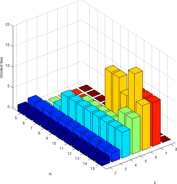
Figure 9: Shortest times achieved for transition fidelities greater than $0.99$ for rings of size $N=5,\dots,15$ and transitions from $1$ to $k=2,\dotsc,\lceil N/2\rceil$

IV CONCLUSIONS AND FUTURE WORK

We have demonstrated how static controls can be used to control the information flow in $\tfrac{1}{2}$-spin rings. Compared to dynamic control, finding static controls is a considerably harder optimization problem due to the complexity of the optimization landscape. Careful selection of initial values and enforcement of the constraints derived from eigenstructure analysis substantially improve the performance of the algorithm. For rings, the constraints enforce symmetries that make the rings more similar to chains, and the timing of transmission peaks for corresponding chains give a good indication of the shortest possible times that can be achieved. Better understanding of the symmetry constraints, their relation to the reachability of target states and the design of global optimization algorithms that utilize the specific structure of the problem may yield even better solutions.

References

- [1] S.A. Wolf et al., Spintronics: A spin-based electronics vision for the future, Science, vol. 294, no. 5546, 2001, pp 1488-1495.
- [2] D.D. Awschalom et al., Quantum spintronics: Engineering and manipulating atom-like spins in semiconductors, Science, vol. 339, no. 6124, 2013, pp 1174-1179.
- [3] E. Jonckheere, F. Langbein and S. Schirmer, Information Transfer Fidelity in Networks of Spins, submitted, preprint arXiv:1408.3765.
- [4] S. Schirmer and F. Langbein, Characterization and Control of Quantum Spin Chains and Rings, Communications, Control and Signal Processing (ISCCSP), 6th International Symposium on, 2014, pp 615-619.
- [5] S.G. Schirmer, P.J. Pemberton-Ross, Fast high-fidelity information transmission through spin-chain quantum wires, Phys. Rev. A vol. 80, no. 3, 2009, 030301.
- [6] X. Wang, P. Pemberton-Ross, S.G. Schirmer, Symmetry and subspace controllability for spin networks with a single-node control, IEEE Trans. Autom. Control vol. 57, no 8, 2012, 1945-1956.
- [7] P. Lohsoonthorn, E. Jonckheere, S. Dalzell, Eigenstructure vs Constrained Design for Hypersoninc Winged Cone, J. Guidance, Control, and Dynamics, vol. 24, No. 4, 2001, pp. 648-658.
- [8] E. Jonckheere, F.C. Langbein, S.G. Schirmer, Curvature of quantum rings, Communications Control and Signal Processing (ISCCSP), 2012 5th International Symposium on, 2012, pp 1-6.
- [9] E. Jonckheere, F.C. Langbein, S.G. Schirmer, Quantum networks: anti-core of spin chains, Quantum Information Processing, vol. 13, no.7, 2014, 1607-1637.
- [10] E. Zahedinejad, S. Schirmer, B.C. Sanders, Evolutionary Algorithms for Hard Quantum Control, Phys. Rev. A vol. 90, 2015, 032310.