The Fermi–Pasta–Ulam system as a model for glasses

Abstract

We show that the standard Fermi–Pasta–Ulam system, with a suitable choice for the interparticle potential, constitutes a model for glasses, and indeed an extremely simple and manageable one. Indeed, it allows one to describe the landscape of the minima of the potential energy and to deal concretely with any one of them, determining the spectrum of frequencies and the normal modes. A relevant role is played by the harmonic energy $\mathcal{E}$ relative to a given minimum, i.e., the expansion of the Hamiltonian about the minimum up to second order. Indeed we find that there exists an energy threshold in $\mathcal{E}$ such that below it the harmonic energy $\mathcal{E}$ appears to be an approximate integral of motion for the whole observation time. Consequently, the system remains trapped near the minimum, in what may be called a vitreous or glassy state. Instead, for larger values of $\mathcal{E}$ the system rather quickly relaxes to a final equilibrium state. Moreover we find that the vitreous states present peculiar statistical behaviors, still involving the harmonic energy $\mathcal{E}$. Indeed, the vitreous states are described by a Gibbs distribution with an effective Hamiltonian close to $\mathcal{E}$ and with a suitable effective inverse temperature. The final equilibrium state presents instead statistical properties which are in very good agreement with the Gibbs distribution relative to the full Hamiltonian of the system.

1 Introduction

If one looks at the microscopic equations of motion, there is essentially no difference between a glass and the corresponding crystal form. They live in the same phase space and have the same Hamiltonian, with a potential energy presenting a huge number of minima. In both cases the initial data lie near one of the potential energy minima, the only peculiarity of the crystal being that the corresponding minimum is the absolute one.

The glass and the corresponding crystal show different physical behaviors just because they remain trapped for an extremely long time in two different regions of phase space (two regions about two different minima, indeed). A final relaxation to global equilibrium might perhaps occur, but only over time scales of a huge magnitude, outside the experimental reach. One can thus conjecture that there exist suitable effective integrals of motion, which forbid the system from exploring the whole a priori available “energy surface”.

This analogy or some variant of it certainly is at the basis of the paper [1] (see also [2]), in which for the first time the idea was advanced that an analogy may exist between the standard Fermi–Pasta–Ulam system [3] and glasses. Indeed it was suggested that the apparent paradox of lack of energy equipartition observed in the FPU system for initial data of FPU type (long wavelength excitations) might be interpreted as analogous to the glass–like trapping of a system near a potential energy minimum. In both cases, a final approach to equilibrium might occur over longer time scales. However, apparently such analogy was no longer pursued.

In the present paper we make explicit such a qualitative analogy, through numerical integrations of a FPU system, i.e., a linear chain of particles with nearest–neighbor interaction. The only peculiarity of the present model is that, for the interaction, a double–well quartic potential is chosen (Fig. 1). This is easily seen to imply a property which is a characteristic feature of the literature on glasses. Namely, that the system possesses a huge number (increasing exponentially with the sistem size) of stable equilibrium points, each corresponding to a disordered configuration of particles, which are usually said to constitute the “potential energy landscape” of the system.

Obviously, the program of understanding glassy dynamics in terms of the potential energy landscape is an old one, which goes back at least to the work of Goldstein [4] and was pursued more recently ib several works (see for example [5]). The advantage of the present model seems to be that in principle it allows one to locate all the equilibrium points, ascertain their stability, and compute for each of them the frequency spectrum (Fig. 2) together with the corresponding normal modes of oscillation (Fig.3). So one has an essentially complete information on the system, at variance with what occurs with three-dimensional models.

Our aim is to exploit such information in studying the dynamics of our model exactly in the spirit of the standard studies on the Fermi–Pasta–Ulam system.

The numerical simulations show that the system admits glassy states: if the initial conditions are chosen sufficiently “near” a local minimum, the trajectory remains trapped in a region about that point for the duration of the simulations. This implies that ergodicity is broken, at least on the times scale of our simulations. In fact we find that there exists another function, besides the total Hamiltonian, which remains practically constant during the evolution. Such a practically constant value is orders of magnitudes different from that of the corresponding phase average. This function is nothing but the sum of the energies of the normal modes relative to the considered equilibrium configuration. In the rest of the paper such a function will be called the “total harmonic energy”, or simply the “harmonic energy”, and denoted by $\mathcal{E}$.

It appears that the harmonic energy $\mathcal{E}$ determines whether the system will be trapped or not: if its value is below a certain threshold the system does not thermalize, analogously to what occurs in the familiar FPU system. Instead, a transition to a behavior of ergodic type occurs if the value of $\mathcal{E}$ is sufficiently raised (Figs. 6 and 7).

Obviously, a trajectory might remain trapped about a local potential minimum because of a trivial reason, i.e.. just in virtue of conservation of the Hamiltonian. But this is not what happens in the case of glasses because, in the thermodynamic limit, there is plenty of energy available for a particle to leap over a potential barrier. It is just in order to insure that this happens also in our model that the double well potential was chosen with a very low barrier between the two minima (Fig. 1). Thus, in all cases in which the system appears to be trapped near a vitreous equilibrium point, the total energy is much larger (by factors of order ten or a hundred, depending on the system size) than the one needed for a particle to leap over the barrier. So, conservation of the Hamiltonian alone cannot explain the trapping. Instead, the trapping is apparently due to the fact that the total harmonic energy $\mathcal{E}$ relative to the considered minimum is practically a constant of motion in a neighborhod about it, whereas this no longer occurs for initial data sufficiently far away from the stable equilibrium point, i.e., above a certain threshold in $\mathcal{E}$.

This is the first result of our paper. A second one pertains to the distribution of the normal mode energies. Indeed, if computed in the equilibrium Gibbs state (through a Montecarlo simulation), such distribution displays a very distinctive character (Fig. 5). We find that the empirical distribution observed in the final eauilibrium state above threshldold agrees very well with the theoretical equilibrium one (see Fig. 8). This is completely at variance with what occurs in the glassy state (below threshold). Indeed in such a case the empirical distribution (see Fig. 9) follows an exponential law of the type $\exp(-\beta_{eff}E)$, This suggests that in the glassy state there exists a (quasi–equilibrium) measure, actually a Gibbs measure $\exp(-\beta_{eff}\tilde{H})$, with a suitable effective Hamiltonian $\tilde{H}$ close to the total harmonic energy $\mathcal{E}$ (relative to the considered minimum), and a suitable effective temperature. This reminds us of what occurs in the description of the different phases met in phase transitions, as was particularly stressed by Frenkel [6].

The paper is organized as follows. In Section 2 we describe the model, determine an equilibrium point and compute the corresponding normal modes of oscillation together with the related spectrum of frequencies. In Section 3 we discuss the statistical features of the equilibrium state. In Section 4 we illustrate the results of our numerical computations, which exhibit the existence of a glassy state in our model. Some final remarks are reported in Section 5.

2 The model, the local minima and the corresponding normal modes

Figure 1: Plot of the two body potential as a function of particle “distance”.

If one considers a linear chain of $N+2$ equal point particles with a nearest neighbor interaction and fixed ends, one gets the following Hamiltonian

$$H=\frac{1}{2m}\sum_{j=1}^{N}p_{j}^{2}+\sum_{j=0}^{N}V(x_{j+1}-x_{j})\ ,$$ (1)

with $x_{0}=0$, $x_{N+1}=L$, where $L$ is the total length of the chain. A trivial equilibrium point is obtained by taking $x_{j+1}-x_{j}=L/(N+1)$, which corresponds to a crystal structure. A more general equilibrium is obtained by imposing that

$$V^{\prime}(x_{j+1}-x_{j})\buildrel{\rm def}\over{=}F(x_{j+1}-x_{j})=b\quad\mbox{for all}\quad j\ ,$$

so that the two forces acting on each particle balance. Now, if $V^{\prime}(r)$ is monotonic, then the crystal equilibrium is the only possible one. Otherwise, if $F^{-1}(b)$ (the inverse image of $b$ under the application of the function $F$) contains $m>1$ points $a_{1},\ldots,a_{m}$, then one gets $m^{N}$ different equilibrium points, which are obtained by choosing in all possible ways the “distances” $r_{j}\buildrel{\rm def}\over{=}x_{j+1}-x_{j}$ between adjacent particles, taking them from the values $a_{l}$. As in the ordered crystal case, $b$ is determined by imposing

$$\sum r_{j}=L\ .$$

Expanding the potential energy about one of these equilibria up to second order one gets

$$V_{tot}=\sum V(r_{j})+\frac{1}{2}\sum V^{\prime\prime}(r_{j})(q_{j+1}-q_{j})^{2}+\dots$$ (2)

where $q_{j}$ is the displacement of the $j$–th particle from its equilibrium position. This shows that if the values $r_{j}$ are such that $V^{\prime\prime}(r_{j})>0$ for all $j$, then the considered equilibrium point is a local minimum, and so is stable. We do not discuss here the general case, and in the present paper we consider only equilibrium points for which the above condition is satisfied. For example, this certainly occurs if the two–body potential $V(r)$ presents two minima, i.e., is a double well potential, and one takes as $r_{j}$ one of them.

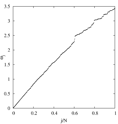
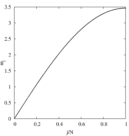
Figure 2: Frequency spectra, i.e., frequencies of the normal modes, about a minimum of the potential energy. Left panel: a glass case (local minimum). Right panel: the crystal case (absolute minimum). In the glassy case the frequencies are reported in ascending order as a function of the index $j/N$. System size is $N=512$.

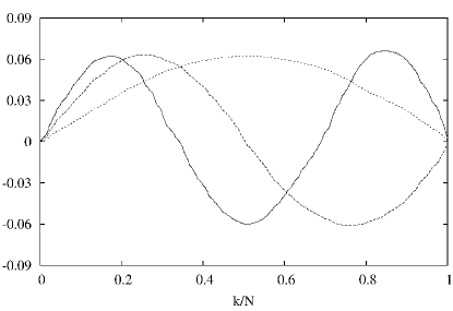
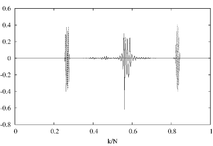
Figure 3: Shapes of the normal modes, namely, of the oscillation amplitudes of the particles as a function of the particle number normalized to 1, for a disordered equilibrium point. System size is $N=512$. Left panel: the three normal modes of lowest frequencies. The shapes are virtually the same as for the crystal. Right panel: three normal modes in the higher part of the frequency spectrum (with frequencies $\omega_{k}=1.93,2.89,3.34$). The localization phenomenon is clearly exhibited.

Clearly each of such equilibrium points corresponds to a disordered structure. Moreover, one meets here in a natural way with a random frame, because each of such equilibria can be obtained by choosing at random the distances $r_{j}$, among the $m$ possible values $a_{l}$. So one obtains a “landscape” of local minima, whose number is exponentially increasing with the number of particles.

For the purpose of discussing such vitreous states, it is of interest to determine the normal modes of a given equilibrium point. In the disordered case this can be obtained only by numerical means, computing the change–of–basis matrix $\hat{U}$ which diagonalizes the dynamical matrix. This forces us to make a definite choice for the two-body potential $V(r)$, which we take within the Fermi–Pasta–Ulam family $V(r)={r^{2}}/2+\alpha r^{3}/3+\beta r^{4}/4$, by fixing $\alpha=-5$ and $\beta=4$, namely,

$$V(r)=\frac{r^{2}}{2}-\frac{5}{3}r^{3}+r^{4}\ .$$ (3)

The graph of the potential is displayed in Fig. 1. As one sees, this is an asymmetric double–well potential, with the ratio between the heigths of the two barriers equal to $\approx 0.05$, and the distance between the minima equal to 1. With a potential of such a type, one might guess that a jump from the higher minimum to the lower one easily occurs. However, our numerical simulations will show that this is not the case.

Having chosen the potential, we determine one among the equilibrium configurations by choosing at random the distances between adjacent particles. We take $r_{j}=1$ with probability $0.64$ and $r_{j}=0$ with probability $0.36$, in order to insure that the total length be $L$. We then compute the change–of–basis matrix $\hat{U}$ and determine the normal modes together with their frequencies. In Fig.2 we report the spectrum of the disordered system (left panel). As the wave number $k$ does not exist in this case, we sort the frequencies in ascending order, i.e., in such a way that $\omega_{j+1}\geq\omega_{j}$. For comparison, we also report in the figure (right panel) the spectrum of the crystalline system, i.e., of the system for which all $r_{j}$’s are equal to $1$. One sees that the spectra are alike for the first part of the spectrum, while qualitative differences show up in the second part, where the disordered spectrum presents some discontinuities.

For what concerns the shapes of the normal modes, some examples are shown in Fig. 3. The low–frequencies modes are delocalized and quite similar to the crystalline case (left panel). Instead, the modes become localized as the frequency increases, and finally, in the upper part of the spectrum, they are localized on only a very few sites (right panel). This is in agreement with the analytical results reported in [7].

3 The statistical approach

We will show in a moment that the vitreous state is not at all typical, i.e., that, if the initial data are taken at random, then the system is far from any equilibrium point. Here ”random” means as usual that the data are extracted according to the Gibbs measure

$$\,\mathrm{d}\mu=\frac{e^{-\beta H(p_{1},\ldots,x_{N})}}{Z(\beta)}\,\mathrm{d}p_{1}\ldots\,\mathrm{d}x_{N}\ .$$ (4)

Care should be taken in choosing a suitable value of $\beta$, if one wants that the mean energy $U$ falls in a range in which an exponentially large number of equilibrium points are present. With our choice of the two–body potential, this occurs if one takes for example $\beta=6$, which is the value we used in all our numerical computations. For such a value of $\beta$ we also computed the average length of the chain with free ends, and fixed the actual length $L$ to such an average value. The value $L$, in turn, determines also the values assigned to the probabilities needed to build up the glass in the way described in the previous section.

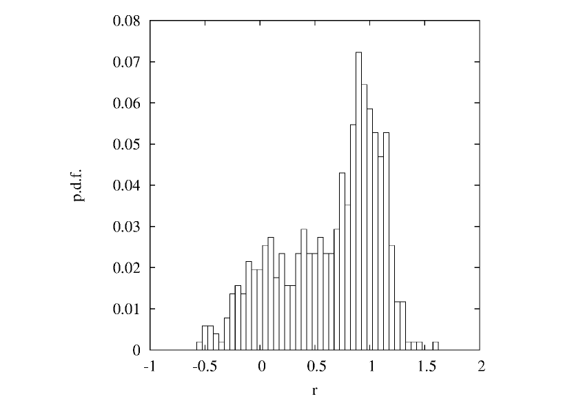
Figure 4: The probability distribution function for the distance between adjacent particles, for a canonical distribution with $\beta=6$.

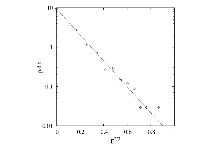
Figure 5: For a canonical distribution with $\beta=6$, plot of the probability distribution function for the energy of the normal modes, versus $E^{2/3}$, in semilogarithmic scale. The continuous line is the function $\exp(-\gamma E^{2/3})$, with $\gamma=7.6$. System size is $N=512$.

So, having fixed $\beta$, one can extract some data, and construct the histogram of the distances $r_{j}$ between adjacent particles. The result is shown in Fig. 4. As one sees, the dispersion is very large. In particular, one has a maximun at $r=1$ and a relative maximum about $r=0$. The large dispersion clearly shows that, in a generic configuration, the particles are not close to any minimum of the potential, so that a vitreous state in non generic.

A different way of describing this situation is by looking at other quantities. In particular one can look at the distribution of the energy of the normal modes relative to a given minimum. This is shown in Fig. 5. One finds a characteristic decay, as the histogram is well approximated by a distribution of the type $\exp(-\gamma E^{2/3})$, with $\gamma=7.6$). This means that the distribution has a heavy tail, which in turn means that many modes have a big energy, i.e., the point in phase space is ”far” (in the energy norm) from the considered equilibrium point. The shape of the histogram is also useful in deciding whether the system did thermalize or not, as will be better explained below.

Thus a vitreous state can only be constructed by hands in the way explained in Section 2, and not by extracting it at random with the Gibbs measure. In other terms, the vitreous states do not belong to the so–called Boltzmann sea (i.e., the set of points of phase space which are ”typical” with respect to the Gibbs measure). Thus, vitreous states can show up only if the dynamics is not ergodic, i.e., only if, placing initially the system near a local equilibrium point, it later remains “frozen” there for a long time without entering into the ”Boltzmann sea”. It is in this sense that ergodicity is, as one often says, “broken”.

We suggest two possible ways to check that the system remains outside the Boltzmann sea. The first is statistical in nature. One chooses an initial datum near the equilibrium point representing the glass, computes the orbit for a certain time, and also computes the histogram of the energies of the single normal modes, at the final time. If such histogram agrees well with the one computed according to the Gibbs distribution, in particular by showing heavy tails, then the system did thermalize, leaving the neighborhood of the equilibrium point. Otherwise the system is still frozen in the glassy state.

A more geometrical approach to control whether the point remains in a neighborhood of the equilibrium point is the following. Starting again from an initial datum near the equilibrium point, one computes the trajectory, and looks at the total harmonic energy $\mathcal{E}$, i.e., at the sum of the energies of the normal modes, as a function of time. The set defined by $\mathcal{E}\leq\delta$, with $\delta$ much smaller than the phase average $\langle\mathcal{E}\rangle$, is a (small) ellipsoid centered at the equilibrium point. If the total harmonic energy $\mathcal{E}$ approaches its phase average, then the system leaves the neighborhood and (possibly) does thermalize.

If instead, during the evolution, the total harmonic energy remains almost constant, close to its initial value, then the motion is confined in such an ellipsoid, and so remains close to the equilibrium point. This shows that the system remains a “glass”. At the same time this shows that ergodicity is broken in the standard sense of dynamical system theory, i.e., there exists a function, independent of the total energy of the system, whose time average does not converge to its phase average.

As said in the Introduction, the aim of this paper is to show, through numerical integrations of the equation of motion, that this actually happens, i.e., that there exists a threshold of the total harmonic energy $\mathcal{E}$ such that, if one starts with a smaller value of $\mathcal{E}$ the system remains “frozen” in the glassy state without thermalizing, up to the times for which we can numerically follow the system. In this sense we recover, in the present setting, the classical results of the standard Fermi–Pasta–Ulam system.

4 Numerical results

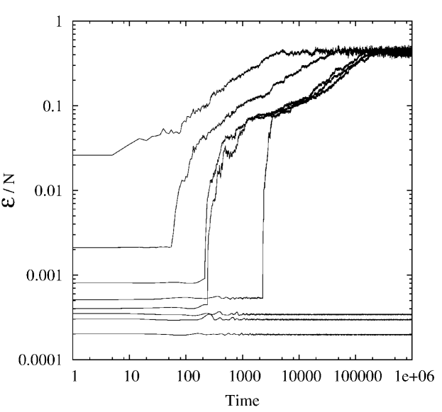
Figure 6: Total harmonic energy per particle $\mathcal{E}/N$ as a function of time, in logarithmic scale. The curves correspond to a system of $N=512$ particles with initial values of $\mathcal{E}/N$ equal to 0.0002, 0.0003, 0.00035, 0.0004, 0.0005, 0.0008, 0.002 and 0.006.

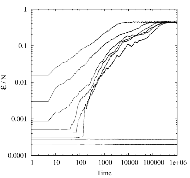
Figure 7: Total harmonic energy per particle $\mathcal{E}/N$ as a function of time, in logarithmic scale. The curves correspond to a system of $N=4096$ particles with initial values of $\mathcal{E}/N$ equal to 0.0002, 0.000275, 0.0003, 0.0004, 0.0005, 0.0008, 0.002 and 0.006.

As explained above, we integrated (by the standard leap–frog method) the equations of motions corresponding to the Hamiltonian (1), with a potential $V(r)$ given by (3). The time step was chosen equal to $0.005$, so as to insure an energy conservation better than a part over a thousand in all the performed computations. The total time of each integration was equal to $10^{6}$.

We integrated the system for two different numbers $N$ of particles, namely, $N=512$ and $N=4096$. For each of such two values of $N$ we constructed a vitreous equilibrium point as described earlier in Section 2. Then the initial data near it were chosen in the familiar way used in the Fermi–Pasta–Ulam model, i.e., by assigning energies and phases to the normal modes pertaining to that equilibrium.

In fact, we chose to excite only low–frequency packets of modes, as done in many numerical studies of the Fermi–Pasta–Ulam system (see [8] or the recent work [9]). More precisely, in the case $N=512$ we excited only the three lowest frequency modes, giving them an equal share of energy, while choosing the phases at random. In the case $N=4096$, we excited only the twenty four lowest–frequency modes, so that the packet had the same relative width as for $N=512$. Again the initial energies were the same for all the excited modes, with the phases chosen at random.

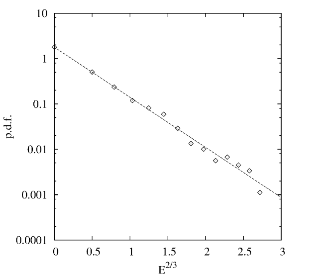
Figure 8: Histogram of the distribution of the mormal mode energies (diamonds), at the end of the numerical integration, in semilogarithmic scale. Initial value of $\mathcal{E}/N$ equal to $0.0008$, a case above threshold. The values are reported versus $E^{2/3}$, as for the theoretical equilibrium p.d.f. reported in Fig. 5. The agreement is evident. The continuous line is the graph of the function $\exp\,(-\gamma E^{2/3})$, with $\gamma=2.54$.

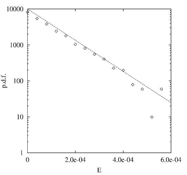
Figure 9: Histogram of the distribution of the mormal mode energies (diamonds), at the end of the integration, in semilogarithmic scale. Initial value of $\mathcal{E}/N$ is $0.0001$, a case below threshold. Values are reported versus $E$. The continuous line is the graph of the function $\exp(-\beta_{eff}E)$, with $1/\beta_{eff}=\mathcal{E}/N=0.0001$. System size is $N=512$.

We made different runs in both cases, with the initial total harmonic energies chosen in such a way that the total harmonic energies per particle $\mathcal{E}/N$ were essentially the same for the two values of $N$. The results are summarized in the Figures 6-9.

In Figure 6, we report the total harmonic energy per particle $\mathcal{E}/N$ as a function of time in logarithmic scale, for the case $N=512$. We report eight runs with different initial values of $\mathcal{E}/N$ in the range $0.0001\div 0.006$. One sees that if the initial value of $\mathcal{E}/N$ is above a threshold (laying between $0.0003\div 0.0004$), the total harmonic energy $\mathcal{E}$ soon starts increasing, and then reaches, after some time, an asymptotic value which agrees rather well with the corresponding phase average computed through the Gibbs measure (with $\beta=6$). In this case the system did thermalize. Below threshold things are different: the total harmonic energy $\mathcal{E}$ remains constant, just fluctuating a bit about its initial value. So below threshold the system is frozen in a glassy state up to the total integration time, and ergodicity is broken, at least on such a time scale. Perhaps the system might thermalize on a longer time scale, but in any case such time scale has to increase sharply, below the threshold.

Things are the same also in the case $N=4096$, as one sees in Figure 7. Even in this case the total harmonic energy $\mathcal{E}$ goes asymptotically to its phase average if the initial value of $\mathcal{E}/N$ is above a threshold (laying now between $0.00025\div 0.0003$) while remaining essentially constant below such a threshold. Notice that the threshold of $\mathcal{E}/N$ appears to depend on the number $N$ of particles, even if not in a quite strong way. However, as the threshold could also exhibit a dependence on the chosen local minimum, the dependence of the threshold on the number $N$ of particles needs to be more carefully investigated. We leave this task for future studies, and in this paper we content ourselves with indicating that the values of the threshold (expressed in terms of energy per particle) have roughly the same order of magnitude in the two cases.

A very interesting fact shows up if one investigates the distribution of the energies of the single normal modes. This is shown in Figure 8–9, which give the histograms for the values of the energies at the final time of integration, The figure refers to $N=512$ (the case $N=4096$ gives the same results, and so the histograms are not reported here). The first figure refers to an initial value of $\mathcal{E}/N$ equal to $0.0008$, a case above threshold. Here the system did thermalize, and in fact one sees that the histogram decays as a stretched exponential, with the same power $E^{2/3}$ as the one computed at equilibrium. Things, instead, are completely different below threshold. This is shown in Figure 9, which corresponds to an initial value of $\mathcal{E}/N$ equal to $0.0001$. Now one sees that the distribution is of the type $\exp(-\beta_{eff}E)$, i.e., of Gibbs type. However, one has now an effective (quadratic) Hamiltonian instead of the true Hamiltonian, and moreover an effective inverse temperature $\beta_{eff}$ with $1/\beta_{eff}=\mathcal{E}/N$, as might have been expected. So it appears as if the glassy state could be described by a measure of Gibbs type with an effective Hamiltonian and an effective temperature. Such a measure is different from the Gibbs one relative to the true hamiltonian, which instead describes the final equilibrium state very far from the glassy state.

5 Final comments

We have shown that, in our Fermi–Pasta–Ulam model with a double–well interparticle potential, it is possible to build a vitreous state which is stable for a very long time. Thus the system fails to exhibit an ergodic behavior on large time scales, in very close analogy with what observed in the original FPU paper.

Now, perhaps this might have been forecast on the basis of the present theoretical understanding of the FPU model, particularly (see for example [10]) for what concerns the slowing down of relaxation to equilibrium. However, the same can not be said concerning the other main result found here for the glassy states, which came as a surprise. Namely, the Gibbs–like form of the histogram of the distribution of the mode energies. This seems to indicate that the measure which describes the glassy state has first of all to be of Gibbs type, with however both an effective Hamiltonian and an effective inverse temperature $\beta_{eff}$, in place of the true Hamiltonian and the true $\beta$. Actually, a phenomelogical approach of this type was taken in the physical literature (see for example [11]). However, a clear theoretical understanding of this point is apparently lacking at the moment.

Another interesting point is that, below threshold, the total harmonic energy $\mathcal{E}$ appears to be a conserved quantity, independest of the total Hamiltonian $H$. Now, in the standard studies on the FPU model, i.e., those concerned with the crystal state, it is usually assumed that $\mathcal{E}$ is conserved because of conservation of the Hamiltonian $H$, the two quantities being very close to each other in that case. So the present results cast some doubts on that belief. The interesting point is that, if $\mathcal{E}$ corresponds to a conserved quantity independent of $H$, then the criterion usually employed for checking thermalization in the FPU system (namely, the occurring or not of equipartition of the normal mode energies) should be reconsidered. Indeed in the case of glasses such a criterion would lead to estimates of the relaxation times much lower than those found here.

References

- [1] R. Fucito, F. Marchesoni, E. Marinari, G. Parisi, L. Peliti, S. Ruffo, A. Vulpiani, Approach to equilibrium in a chain of nonlinear oscillators, J. Phys. 43, 707 (1982).
- [2] G. Parisi, On the approach to equilibrium of a Hamiltonian chain of anharmonic oscillators, Europhys. Lett. 40, 357 (1997).
- [3] E. Fermi, J. Pasta, S. Ulam, Studies of nonlinear problems, in E. Fermi, Collected Papers, Vol. II, No 266, page 977, Accademia Nazionale dei Lincei and The University of Chicago Press, Chicago (1965).
- [4] M. Goldstein, Viscous liquids and the glass transition: a potential energy barrier picture, J. Chem. Phys. 51, 3728 (1969).
- [5] T.S. Grigera, A. Cavagna, I. Giardina, G. Parisi, Geomwetric approach to the dynamic glass transition, Phys. Rev. Lett. 88, 055502 (2002).
- [6] J. Frenkel, Kinetic theory of liquids, Oxford C.P., Oxford (1946).
- [7] R. Carmona, A. Klein, F. Martinelli, Anderson localization for Bernoulli and other singular potentials, Commun. Mat. Phys. 108, 41 (1987).
- [8] G. Benettin, A. Carati, L. Galgani, A. Giorgilli, The Fermi–Pasta–Ulam problem and the metastability perspective, in The Fermi-Pasta-Ulam Problem: A Status Report, G. Gallavotti ed., Lecture Notes in Physics , Vol. 728, Springer Verlag, Berlin (2007).
- [9] G. Benettin, A. Ponno, Time scales to equipartition in the Fermi–Pasta–Ulam problem: finite size effects and thermodynamic limit, J. Stat. Phys. 144, 793 (2011).
- [10] A. Maiocchi, D. Bambusi, A. Carati, An averaging theorem for Fermi–Pasta–Ulam in the thermodynamic limit, J. Stat. Phys. 155, 300 (2014).
- [11] R.C. Lord, J.C. Morrow, Calculation of the heat capacity of –quartz and vitreous silica from spectroscopic data, J. Chem. Phys. 26, 230 (1957).