Global Convergence of Non-Convex Gradient Descent for Computing Matrix Squareroot

Abstract

While there has been a significant amount of work studying gradient descent techniques for non-convex optimization problems over the last few years, all existing results establish either local convergence with good rates or global convergence with highly suboptimal rates, for many problems of interest. In this paper, we take the first step in getting the best of both worlds – establishing global convergence and obtaining a good rate of convergence for the problem of computing squareroot of a positive definite (PD) matrix, which is a widely studied problem in numerical linear algebra with applications in machine learning and statistics among others.

Given a PD matrix $\mathbf{M}$ and a PD starting point $\mathbf{U_{0}}$, we show that gradient descent with appropriately chosen step-size finds an $\epsilon$-accurate squareroot of $\mathbf{M}$ in $\mathcal{O}\left(\alpha\log(\left\|\mathbf{M}-\mathbf{U_{0}}^{2}\right\|_{F}/\epsilon)\right)$ iterations, where $\alpha\stackrel{{\scriptstyle\triangle}}{{=}}(\max\{\left\|{\mathbf{U_{0}}}\right\|_{2}^{2},\left\|{\mathbf{M}}\right\|_{2}\}$ $/$ $\min\{\sigma_{\min}^{2}(\mathbf{U_{0}}),\sigma_{\min}\left(\mathbf{M}\right)\})^{3/2}$. Our result is the first to establish global convergence for this problem and that it is robust to errors in each iteration. A key contribution of our work is the general proof technique which we believe should further excite research in understanding deterministic and stochastic variants of simple non-convex gradient descent algorithms with good global convergence rates for other problems in machine learning and numerical linear algebra.

1 Introduction

Given that a large number of problems and frameworks in machine learning are non-convex optimization problems (examples include non-negative matrix factorization (Lee and Seung, 2001), sparse coding (Aharon et al., 2006), matrix sensing (Recht et al., 2010), matrix completion (Koren et al., 2009), phase retrieval (Netrapalli et al., 2015) etc.), in the last few years, there has been an increased interest in designing efficient non-convex optimization algorithms. Several recent works establish local convergence to the global optimum for problems such as matrix sensing (Jain et al., 2013; Tu et al., 2015), matrix completion (Jain and Netrapalli, 2014; Sun and Luo, 2015), phase retrieval (Candes et al., 2015), sparse coding (Agarwal et al., 2013) and so on (and hence, require careful initialization). However, despite strong empirical evidence, none of these results have been able to establish global convergence. On the other hand some other recent works (Nesterov and Polyak, 2006; Ge et al., 2015; Lee et al., 2016; Sun et al., 2015) establish the global convergence of gradient descent methods to local minima for a large class of non-convex problems but the results they obtain are quite suboptimal compared to the local convergence results mentioned above. In other words, results that have very good rates are only local (and results that are global do not have very good rates).

Therefore, a natural and important question is if gradient descent actually has a good global convergence rate when applied to specific and important functions that are of interest in machine learning. Apart from theoretical implications, such a result is also important in practice since a) finding a good initialization might be difficult and b) local convergence results are inherently difficult to extend to stochastic algorithms due to noise.

In this work, we answer the above question in affirmative for the problem of computing square root of a positive definite (PD) matrix $\mathbf{M}$: i.e., $\min_{\mathbf{U}\succeq 0}f(\mathbf{U})$ where $f(\mathbf{U})=\|\mathbf{M}-\mathbf{U}^{2}\|_{F}^{2}$. This problem in itself is a fundamental one and arises in several contexts such as computation of the matrix sign function (Higham, 2008), computation of data whitening matrices, signal processing applications (Kaminski et al., 1971; Carlson, 1990; Van Der Merwe and Wan, 2001; Tippett et al., 2003) and so on.

1.1 Related work

Given the importance of computing the matrix squareroot, there has been a tremendous amount of work in the numerical linear algebra community focused on this problem (Björck and Hammarling, 1983; Higham, 1986, 1987, 1997; Meini, 2004). For a detailed list of references, see Chapter 6 in Higham’s book (Higham, 2008).

The basic component of most these algorithms is the Newton’s method to find the square root of a positive number. Given a positive number $m$ and a positive starting point ${u_{0}}$, Newton’s method gives rise to the iteration

$${u_{t+1}}\leftarrow\frac{1}{2}\left({u_{t}}+\frac{m}{{u_{t}}}\right).$$ (1)

It can be shown that the iterates converge to $\sqrt{m}$ at a quadratic rate (i.e., $\epsilon$-accuracy in $\log\log\frac{1}{\epsilon}$ iterations). The extension of this approach to the matrix case is not straight forward due to non commutativity of matrix multiplication. For instance, if $\mathbf{M}$ and $\mathbf{U_{t}}$ were matrices, it is not clear if $\frac{m}{{u_{t}}}$ should be replaced by ${\mathbf{U_{t}}}^{-1}\mathbf{M}$ or $\mathbf{M}{\mathbf{U_{t}}}^{-1}$ or something else. One approach to overcome this issue is to select $\mathbf{U_{0}}$ carefully to ensure commutativity through all iterations (Higham, 1986, 1997; Meini, 2004), for example, $\mathbf{U_{0}}=\mathbf{M}$ or $\mathbf{U_{0}}=\mathbf{I}$. However, commutativity is a brittle property and small numerical errors in an iteration itself can result in loss of commutativity. Although a lot of work since, has focused on designing stable iterations that are inspired by Eq.(1) (Higham, 1986, 1997; Meini, 2004), and has succeeded in making it robust in practice, no provable robustness guarantees are known in the presence of repeated errors. Similarly, another recent approach by  Sra (2015) uses geometric optimization to solve the matrix squareroot problem but their analysis also does not address the stability or robustness to numerical or statistical errors (if we see a noisy version of $\mathbf{M}$) .

Another approach to solve the matrix square-root problem is to use the eigenvalue decomposition (EVD) and then take square-root of the eigenvalues. To the best of our knowledge, state-of-the-art computation complexity for computing the EVD of a matrix (in the real arithmetic model of computation) is due to Pan et al. (1998), which is $\mathcal{O}\left(n^{{\omega}}\log n+n\log^{2}n\log\log\frac{1}{\epsilon}\right)$ for matrices with distinct eigenvalues. Though the result is close to optimal (in reducing the EVD to matrix multiplication), the algorithm and the analysis are quite complicated. For instance robustness of these methods to errors is not well understood. As mentioned above however, our focus is to understand if local search techniques like gradient descent (which are often applied to several non-convex optimization procedures) indeed avoid saddle points and local minima, and can guide the solution to global optimum.

As we mentioned earlier, Ge et al. (2015); Lee et al. (2016) give some recent results on global convergence for general non-convex problems which can be applied to matrix squareroot problem. While Lee et al. (2016) prove only asymptotic behavior of gradient descent without any rate, applying the result of Ge et al. (2015) gives us a runtime of $\mathcal{O}\left(n^{10}/\textrm{poly}\left(\epsilon\right)\right)$, which is highly suboptimal in terms of its dependence on $n$ and $\epsilon$.

Finally, we note that subsequent to this work, Jin et al. (2017) proved global convergence results with almost sharp dimension dependence for a much wider class of functions. While Jin et al. (2017) explicitly add perturbation to help escape saddle points, our framework does not require perturbation, and shows that for this problem, gradient descent naturally stays away from saddle points.

1.2 Our contribution

Method	Runtime	Global convergence	Provable robustness
Gradient descent (this paper)	$\mathcal{O}\left(\alpha n^{{\omega}}\log\frac{1}{\epsilon}\right)$	$\checkmark$	$\checkmark$
Stochastic gradient descent (Ge et al., 2015)	$\mathcal{O}\left(n^{10}/\textrm{poly}\left(\epsilon\right)\right)$	$\checkmark$	$\checkmark$
Newton variants (Higham, 2008)	$\mathcal{O}\left(n^{{\omega}}\log\log\frac{1}{\epsilon}\right)$	$\times$	$\times$
EVD (algebraic (Pan et al., 1998))	$\mathcal{O}\left(n^{{\omega}}\log n+n\log^{2}n\log\log\frac{1}{\epsilon}\right)$	Not iterative	$\times$
EVD (power method (Golub and Van Loan, 2012))	$\mathcal{O}\left(n^{3}\log\frac{1}{\epsilon}\right)$	Not iterative	$\times$

Table 1: Comparison of our result to existing ones. Here $\omega$ is the matrix multiplication exponent and $\alpha$ is our convergence rate parameter defined in Eq.(3). We show that our method enjoys global convergence and is also provably robust to arbitrary bounded errors in each iteration. In contrast, Newton variants only have local convergence and their robustness to errors in multiple iterations is not known. Robustness of methods based on eigenvalue decomposition is also not well understood.

In this paper, we propose doing gradient descent on the following non-convex formulation:

$$\min_{\mathbf{U}\in\mathbb{R}^{n\times n};\mathbf{U}\succeq 0}\left\|\mathbf{M}-\mathbf{U}^{2}\right\|_{F}^{2}.$$ (2)

We show that if the starting point $\mathbf{U_{0}}$ is chosen to be a positive definite matrix, our algorithm converges to the global optimum of Eq.(2) at a geometric rate. In order to state our runtime, we make the following notation:

$$\alpha\stackrel{{\scriptstyle\triangle}}{{=}}\left(\frac{\max\left(\left\|{\mathbf{U_{0}}}\right\|_{2},\sqrt{\left\|{\mathbf{M}}\right\|_{2}}\right)}{\min\left(\sigma_{\min}\left(\mathbf{U_{0}}\right),\sqrt{\sigma_{\min}\left(\mathbf{M}\right)}\right)}\right)^{3},$$ (3)

where $\sigma_{\min}\left(\mathbf{U_{0}}\right)$ and $\left\|{\mathbf{U_{0}}}\right\|_{2}$ are the minimum singular value and operator norm respectively of the starting point $\mathbf{U_{0}}$, and $\sigma_{\min}\left(\mathbf{M}\right)$ and $\left\|{\mathbf{M}}\right\|_{2}$ are those of $\mathbf{M}$. Our result says that gradient descent converges $\epsilon$ close to the optimum of Eq.(2) in $\mathcal{O}\left(\alpha\log\frac{\left\|\mathbf{M}-\mathbf{U_{0}}^{2}\right\|_{F}}{\epsilon}\right)$ iterations. Each iteration involves doing only three matrix multiplications and no inversions or leastsquares. So the total runtime of our algorithm is $\mathcal{O}\left(n^{{\omega}}\alpha\log\frac{\left\|\mathbf{M}\right\|_{F}}{\epsilon}\right)$, where $\omega<2.373$ is the matrix multiplication exponent(Williams, 2012). As a byproduct of our global convergence guarantee, we obtain the robustness of our algorithm to numerical errors for free. In particular, we show that our algorithm is robust to errors in multiple steps in the sense that if each step has an error of at most $\delta$, then our algorithm achieves a limiting accuracy of $\mathcal{O}\left(\alpha\sqrt{\left\|{\mathbf{M}}\right\|_{2}}\delta\right)$. Another nice feature of our algorithm is that it is based purely on matrix multiplications, where as most existing methods require matrix inversion or solving a system of linear equations. An unsatisfactory part of our result however is the dependence on $\alpha\geq\kappa^{3/2}$, where $\kappa$ is the condition number of $\mathbf{M}$. We prove a lower bound of $\Omega\left(\kappa\right)$ iterations for our method which tells us that the dependence on problem parameters in our result is not a weakness in our analysis.

Outline: In Section 2, we will briefly set up the notation we will use in this paper. In Section 3, we will present our algorithm, approach and main results. We will present the proof of our main result in Section 4 and conclude in Section 5. The proofs of remaining results can be found in the Appendix.

2 Notation

Let us briefly introduce the notation we will use in this paper. We use boldface lower case letters ($\mathbf{v},\mathbf{w},\ldots$) to denote vectors and boldface upper case letters ($\mathbf{M},\mathbf{X},\ldots$) to denote matrices. $\mathbf{M}$ denotes the input matrix we wish to compute the squareroot of. $\sigma_{i}\left(\mathbf{A}\right)$ denotes the $i^{\textrm{th}}$ singular value of $\mathbf{A}$. $\sigma_{\min}\left(\mathbf{A}\right)$ denotes the smallest singular value of $\mathbf{A}$. $\kappa\left(\mathbf{A}\right)$ denotes the condition number of $\mathbf{A}$ i.e., $\frac{\left\|{\mathbf{A}}\right\|_{2}}{\sigma_{\min}\left(\mathbf{A}\right)}$. $\kappa$ without an argument denotes $\kappa\left(\mathbf{M}\right)$. $\lambda_{i}\left(\mathbf{A}\right)$ denotes the $i^{\textrm{th}}$ largest eigenvalue of $\mathbf{A}$ and $\lambda_{\textrm{min}}(\mathbf{A})$ denotes the smallest eigenvalue of $\mathbf{A}$.

3 Our Results

In this section, we present our guarantees and the high-level approach for the analysis of Algorithm 1 which is just gradient descent on the non-convex optimization problem:

$$\min_{\mathbf{U}\in\mathbb{R}^{n\times n};\mathbf{U}\succeq 0}\left\|\mathbf{M}-\mathbf{U}^{2}\right\|_{F}^{2}.$$ (4)

Algorithm 1 Gradient descent for matrix square root

0:  $\mathbf{M}$, PD matrix $\mathbf{U_{0}},\eta,T$

0:  $\mathbf{U}$

  for $t=0,\cdots,T-1$ do

     $\mathbf{U_{t+1}}=\mathbf{U_{t}}-\eta\left(\mathbf{U_{t}}^{2}-\mathbf{M}\right)\mathbf{U_{t}}-\eta\mathbf{U_{t}}\left(\mathbf{U_{t}}^{2}-\mathbf{M}\right)$

  end for

  Return $\mathbf{U_{T}}$.

We first present a warmup analysis, where we assume that all the iterates of Algorithm 1 commute with $\mathbf{M}$. Later, in Section 3.2 we present our approach to analyze Algorithm 1 for any general starting point $\mathbf{U_{0}}$. We provide formal guarantees in Section 3.3.

3.1 Warmup – Analysis with commutativity

In this section, we will give a short proof of convergence for Algorithm 1, when we ensure that all iterates commute with $\mathbf{M}$.

Lemma 3.1.

There exists a constant $c$ such that if $\eta<\frac{c}{\left\|{\mathbf{M}}\right\|_{2}}$, and $\mathbf{U_{0}}$ is chosen to be $\sqrt{\left\|{\mathbf{M}}\right\|_{2}}\cdot\mathbf{I}$, then $\mathbf{U_{t}}$ in Algorithm 1 satisfies:

$$\left\|\mathbf{U_{t}}^{2}-\mathbf{M}\right\|_{F}^{2} \leq\exp\left(-2\eta\sigma_{\min}\left(\mathbf{M}\right)t\right)\left\|\mathbf{U_{0}}^{2}-\mathbf{M}\right\|_{F}^{2}.$$

Proof.

Since $\mathbf{U_{0}}=\sqrt{\left\|{\mathbf{M}}\right\|_{2}}\mathbf{I}$ has the same eigenvectors as $\mathbf{M}$, it can be seen by induction that $\mathbf{U_{t}}$ has the same eigenvectors as $\mathbf{M}$ for every $t$. Every singular value $\sigma_{i}\left(\mathbf{U_{t+1}}\right)$ can be written as

$$\sigma_{i}\left(\mathbf{U_{t+1}}\right)=\left(1-2\eta\left(\sigma_{i}\left(\mathbf{U_{t}}\right)^{2}-\sigma_{i}\left(\mathbf{M}\right)\right)\right)\sigma_{i}\left(\mathbf{U_{t}}\right).$$ (5)

Firstly, this tells us that $\left\|{\mathbf{U_{t}}}\right\|_{2}<\sqrt{2\left\|{\mathbf{M}}\right\|_{2}}$ for every $t$. Verifying this is easy using induction. The statement holds for $t=0$ by hypothesis. Assuming it holds for $\mathbf{U_{t}}$, the induction step follows by considering the two cases $\left\|{\mathbf{U_{t}}}\right\|_{2}\leq\sqrt{\left\|{\mathbf{M}}\right\|_{2}}$ and $\sqrt{\left\|{\mathbf{M}}\right\|_{2}}<\left\|{\mathbf{U_{t}}}\right\|_{2}<\sqrt{2\left\|{\mathbf{M}}\right\|_{2}}$ separately and using the assumption that $\eta<\frac{c}{\left\|{\mathbf{M}}\right\|_{2}}$. A similar induction argument also tells us that $\sigma_{i}\left(\mathbf{U_{t}}\right)>\sqrt{\frac{\sigma_{i}\left(\mathbf{M}\right)}{2}}$. Eq.(5) can now be used to yield the following convergence equation:

$$\left|\sigma_{i}\left(\mathbf{U_{t+1}}\right)^{2}-\sigma_{i}\left(\mathbf{M}\right)\right|$$

$$= \left|\sigma_{i}\left(\mathbf{U_{t}}\right)^{2}-\sigma_{i}\left(\mathbf{M}\right)\right|\cdot\left(1-4\eta\sigma_{i}\left(\mathbf{U_{t}}\right)^{2}\right.$$

$$\quad\quad\quad\left.+4\eta^{2}\sigma_{i}\left(\mathbf{U_{t}}\right)^{2}\left(\sigma_{i}\left(\mathbf{U_{t}}\right)^{2}-\sigma_{i}\left(\mathbf{M}\right)\right)\right)$$

$$\leq \left|\sigma_{i}\left(\mathbf{U_{t}}\right)^{2}-\sigma_{i}\left(\mathbf{M}\right)\right|\cdot\left(1-4\eta\sigma_{i}\left(\mathbf{U_{t}}\right)^{2}\right.$$

$$\quad\quad\quad\left.+8\eta^{2}\sigma_{i}\left(\mathbf{U_{t}}\right)^{2}\left\|{\mathbf{M}}\right\|_{2}\right)$$

$$\leq \left(1-2\eta\sigma_{i}\left(\mathbf{U_{t}}\right)^{2}\right)\left|\sigma_{i}\left(\mathbf{U_{t}}\right)^{2}-\sigma_{i}\left(\mathbf{M}\right)\right|$$

$$\leq \exp\left(-\eta\sigma_{\min}\left(\mathbf{M}\right)\right)\left|\sigma_{i}\left(\mathbf{U_{t}}\right)^{2}-\sigma_{i}\left(\mathbf{M}\right)\right|,$$

where we used the hypothesis on $\eta$ in the last two steps. Using induction gives us

$$\left|\sigma_{i}\left(\mathbf{U_{t}}\right)^{2}-\mathbf{M}\right|\leq\exp\left(-\eta\sigma_{\min}\left(\mathbf{M}\right)t\right)\left|\sigma_{i}\left(\mathbf{U_{0}}\right)^{2}-\mathbf{M}\right|.$$

This can now be used to prove the lemma:

$$\left\|\mathbf{U_{t}}^{2}-\mathbf{M}\right\|_{F}^{2}=\sum_{i}\left(\sigma_{i}\left(\mathbf{U_{t}}\right)^{2}-\sigma_{i}\left(\mathbf{M}\right)\right)^{2}$$

$$\leq \exp\left(-2\eta\sigma_{\min}\left(\mathbf{M}\right)t\right)\sum_{i}\left(\sigma_{i}\left(\mathbf{U_{0}}\right)^{2}-\sigma_{i}\left(\mathbf{M}\right)\right)^{2}$$

$$\leq \exp\left(-2\eta\sigma_{\min}\left(\mathbf{M}\right)t\right)\left\|\mathbf{U_{0}}^{2}-\mathbf{M}\right\|_{F}^{2}.$$

∎

Note that the above proof crucially used the fact that the eigenvectors of $\mathbf{U_{t}}$ and $\mathbf{M}$ are aligned, to reduce the matrix iterations to iterations only over the singular values.

3.2 Approach

As we begin to investigate the global convergence properties of Eq.(4), the above argument breaks down due to lack of alignment between the singular vectors of $\mathbf{M}$ and those of the iterates $\mathbf{U_{t}}$. Let us now take a step back and consider non-convex optimization in general. There are two broad reasons why local search approaches fail for these problems. The first is the presence of local minima and the second is the presence of saddle points. Each of these presents different challenges: with local minima, local search approaches have no way of certifying whether the convergence point is a local minimum or global minimum; while with saddle points, if the iterates get close to a saddle point, the local neighborhood looks essentially flat and escaping the saddle point may take exponential time.

The starting point of our work is the realization that the non-convex formulation of the matrix squareroot problem does not have any local minima. This can be argued using the continuity of the matrix squareroot function, and this statement is indeed true for many matrix factorization problems. The only issue to be contended with is the presence of saddle points. In order to overcome this issue, it suffices to show that the iterates of the algorithm never get too close to a saddle point. More concretely, while optimizing a function $f$ with iterates $\mathbf{U_{t}}$, it suffices to show that for every $t$, $\mathbf{U_{t}}$ always stay in some region $\mathcal{D}$ far from saddle points so that for all $\mathbf{U},\mathbf{U}^{\prime}\in\mathcal{D}$:

$$\left\|\bigtriangledown f(\mathbf{U})-\bigtriangledown f(\mathbf{U}^{\prime})\right\|_{F}\leq L\left\|\mathbf{U}-\mathbf{U}^{\prime}\right\|_{F}$$ (6)

$$\left\|\bigtriangledown f(\mathbf{U})\right\|_{F}\geq\sqrt{\ell\left(f(\mathbf{U})-f_{*}\right)},$$ (7)

where $f_{*}=\min_{\mathbf{U}}f(\mathbf{U})$, and $L$ and $\ell$ are some constants. If we flatten matrix $\mathbf{U}$ to be $n^{2}$-dimensional vector, then Eq.(6) is the standard smoothness assumption in optimization, and Eq.(7) is known as gradient dominated property (Polyak, 1963; Nesterov and Polyak, 2006). If Eq.(6) and Eq.(7) hold, it follows from standard analysis that gradient descent with a step size $\eta<\frac{1}{L}$ achieves geometric convergence with

$$f(\mathbf{U_{t}})-f_{*}\leq\exp\left(-\eta\ell t/2\right)\left(f(\mathbf{U_{0}})-f_{*}\right).$$

Since the gradient in our setting is $\left(\mathbf{U_{t}}^{2}-\mathbf{M}\right)\mathbf{U_{t}}+\mathbf{U_{t}}\left(\mathbf{U_{t}}^{2}-\mathbf{M}\right)$, in order to establish Eq.(7), it suffices to lower bound $\lambda_{\min}\left(\mathbf{U_{t}}\right)$. Similarly, in order to establish Eq.(6), it suffices to upper bound $\left\|{\mathbf{U_{t}}}\right\|_{2}$. Of course, we cannot hope to converge if we start from a saddle point. In particular Eq.(7) will not hold for any $l>0$. The core of our argument consists of Lemmas 4.3 and 4.2, which essentially establish Eq.(6) and Eq.(7) respectively for the matrix squareroot problem Eq.(4), with the resulting parameters $l$ and $L$ dependent on the starting point $\mathbf{U_{0}}$. Lemmas 4.3 and 4.2 accomplish this by proving upper and lower bounds respectively on $\left\|{\mathbf{U_{t}}}\right\|_{2}$ and $\lambda_{\min}\left(\mathbf{U_{t}}\right)$. The proofs of these lemmas use only elementary linear algebra and we believe such results should be possible for many more matrix factorization problems.

3.3 Guarantees

In this section, we will present our main results establishing that gradient descent on (4) converges to the matrix square root at a geometric rate and its robustness to errors in each iteration.

3.3.1 Noiseless setting

The following theorem establishes geometric convergence of Algorithm 1 from a full rank initial point.

Theorem 3.2.

There exist universal numerical constants $c$ and $\widehat{c}$ such that if $\mathbf{U_{0}}$ is a PD matrix and $\eta<\frac{c}{\alpha\beta^{2}}$, then for every $t\in[T-1]$, we have $\mathbf{U_{t}}$ be a PD matrix with

$$\left\|\mathbf{M}-\mathbf{U_{t}}^{2}\right\|_{F}\leq\exp\left(-\widehat{c}\eta\beta^{2}t\right)\left\|\mathbf{M}-\mathbf{U_{0}}^{2}\right\|_{F},$$

where $\alpha$ and $\beta$ are defined as

$$\alpha \stackrel{{\scriptstyle\triangle}}{{=}}\left(\frac{\max\left(\left\|{\mathbf{U_{0}}}\right\|_{2},\sqrt{\left\|{\mathbf{M}}\right\|_{2}}\right)}{\min\left(\sigma_{\min}\left(\mathbf{U_{0}}\right),\sqrt{\sigma_{\min}\left(\mathbf{M}\right)}\right)}\right)^{3},$$

$$\beta \stackrel{{\scriptstyle\triangle}}{{=}}\min\left(\sigma_{\min}\left(\mathbf{U_{0}}\right),\sqrt{\sigma_{\min}\left(\mathbf{M}\right)}\right)$$

Remarks:

• This result implies global geometric convergence. Choosing $\eta=\frac{c}{\alpha\beta^{2}}$, in order to obtain an accuracy of $\epsilon$, the number of iterations required would be $\mathcal{O}\left(\alpha\log\frac{\left\|\mathbf{M}-\mathbf{U_{0}}^{2}\right\|_{F}}{\epsilon}\right)$.

• Note that saddle points of (4) must be rank degenerate matrix ($\sigma_{\min}(\mathbf{U})=0$) and starting Algorithm 1 from a point close to the rank degenerate surface takes a long time to get away from the saddle surface. Hence, as $\mathbf{U_{0}}$ gets close to being rank degenerate, convergence rate guaranteed by Theorem 3.2 degrades (as $\kappa\left(\mathbf{U_{0}}\right)^{3}$). It is possible to obtain a smoother degradation with a finer analysis, but in the current paper, we trade off optimal results for a simple analysis.

• The convergence rate guaranteed by Theorem 3.2 also depends on the relative scales of $\mathbf{U_{0}}$ and $\mathbf{M}$ (say as measured by $\left\|{\mathbf{U_{0}}}\right\|_{2}^{2}/\left\|{\mathbf{M}}\right\|_{2}$) and is best if it is close to $1$.

• We believe that it is possible to extend our analysis to the case where $\mathbf{M}$ is low rank (PSD). In this case, suppose $\text{rank}(\mathbf{M})=k$, and let $\mathbf{U}^{\star}$ be the k-dimensional subspace in which $\mathbf{M}$ resides. Then, saddle points should satisfy $\sigma_{k}({\mathbf{U}}^{\top}\mathbf{U}^{\star})=0$.

A simple corollary of this result is when we choose $\mathbf{U_{0}}=\lambda\mathbf{I}$, where $\left\|{\mathbf{M}}\right\|_{2}\leq\lambda\leq 2\left\|{\mathbf{M}}\right\|_{2}$ (such a $\lambda$ can be found in time $\mathcal{O}\left(n^{2}\right)$ Musco and Musco (2015)).

Corollary 3.3.

Suppose we choose $\mathbf{U_{0}}=\lambda\mathbf{I}$, where $\left\|{\mathbf{M}}\right\|_{2}\leq\lambda\leq 2\left\|{\mathbf{M}}\right\|_{2}$. Then $\left\|\mathbf{M}-\mathbf{U_{T}}^{2}\right\|_{F}\leq\epsilon$ for $T\geq\mathcal{O}\left(\kappa^{\frac{3}{2}}\log\frac{\left\|\mathbf{M}-\mathbf{U_{0}}^{2}\right\|_{F}}{\epsilon}\right)$.

3.3.2 Noise Stability

Theorem 3.2 assumes that the gradient descent updates are performed with out any error. This is not practical. For instance, any implementation of Algorithm 1 would incur rounding errors. Our next result addresses this issue by showing that Algorithm 1 is stable in the presence of small, arbitrary errors in each iteration. This will establish the stability of our algorithm in the presence of round-off errors for instance. Formally, we consider in every gradient step, we incur an error $\mathbf{\bigtriangleup_{t}}$.

The following theorem shows that as long as the errors $\mathbf{\bigtriangleup_{t}}$ are small enough, Algorithm 1 recovers the true squareroot upto an accuracy of the error floor. The proof of the theorem follows fairly easily from that of Theorem 3.2.

Theorem 3.4.

There exist universal numerical constants $c$ and $\widehat{c}$ such that the following holds: Suppose $\mathbf{U_{0}}$ is a PD matrix and $\eta<\frac{c}{\alpha\beta^{2}}$ where $\alpha$ and $\beta$ are defined as before:

$$\alpha \stackrel{{\scriptstyle\triangle}}{{=}}\left(\frac{\max\left(\left\|{\mathbf{U_{0}}}\right\|_{2},\sqrt{\left\|{\mathbf{M}}\right\|_{2}}\right)}{\min\left(\sigma_{\min}\left(\mathbf{U_{0}}\right),\sqrt{\sigma_{\min}\left(\mathbf{M}\right)}\right)}\right)^{3},$$

$$\beta \stackrel{{\scriptstyle\triangle}}{{=}}\min\left(\sigma_{\min}\left(\mathbf{U_{0}}\right),\sqrt{\sigma_{\min}\left(\mathbf{M}\right)}\right).$$

Suppose further that $\left\|{\mathbf{\bigtriangleup_{t}}}\right\|_{2}<\frac{1}{300}\eta{\sigma_{\min}\left(\mathbf{M}\right)}\beta$. Then, for every $t\in[T-1]$, we have $\mathbf{U_{t}}$ be a PD matrix with

$$\left\|\mathbf{M}-\mathbf{U_{t}}^{2}\right\|_{F}\leq\exp\left(-\widehat{c}\eta\beta^{2}t\right)\left\|\mathbf{M}-\mathbf{U_{0}}^{2}\right\|_{F}$$

$$\quad+4\max(\left\|{\mathbf{U_{0}}}\right\|_{2},\sqrt{3\left\|{\mathbf{M}}\right\|_{2}})\sum_{s=0}^{t-1}e^{-\widehat{c}\eta\beta^{2}(t-s-1)}\left\|\mathbf{\bigtriangleup_{s}}\right\|_{F}.$$

Remarks:

• Since the errors above are multiplied by a decreasing sequence, they can be bounded to obtain a limiting accuracy of $\mathcal{O}\left(\alpha(\left\|{\mathbf{U_{0}}}\right\|_{2}+\sqrt{\left\|{\mathbf{M}}\right\|_{2}})(\sup_{s}\left\|\mathbf{\bigtriangleup_{s}}\right\|_{F})\right)$.

• If there is error in only the first iteration i.e., $\mathbf{\bigtriangleup_{t}}=0$ for $t\neq 0$, then the initial error $\mathbf{\bigtriangleup_{0}}$ is attenuated with every iteration,

  $$\left\|\mathbf{M}-\mathbf{U_{t}}^{2}\right\|_{F}\leq\exp\left(-\widehat{c}\eta\beta^{2}t\right)\left\|\mathbf{M}-\mathbf{U_{0}}^{2}\right\|_{F}$$

  $$\quad\quad\quad+6\max(\left\|{\mathbf{U_{0}}}\right\|_{2}^{2},{\left\|{\mathbf{M}}\right\|_{2}})e^{-\widehat{c}\eta\beta^{2}(t-1)}\left\|\mathbf{\bigtriangleup_{0}}\right\|_{F}.$$

  That is, our dependence on $\left\|\mathbf{\bigtriangleup_{0}}\right\|_{F}$ is exponentially decaying with respect to time $t$. On the contrary, best known results only guarantees the error dependence on $\left\|\mathbf{\bigtriangleup_{0}}\right\|_{F}$ will not increase significantly with respect to time $t$ (Higham, 2008).

3.3.3 Lower Bound

We also prove the following lower bound showing that gradient descent with a fixed step size requires $\Omega\left(\kappa\right)$ iterations to achieve an error of $\mathcal{O}\left(\sigma_{\min}\left(\mathbf{M}\right)\right)$.

Theorem 3.5.

For any value of $\kappa$, we can find a matrix $\mathbf{M}$ such that, for any step size $\eta$, there exists an initialization $\mathbf{U_{0}}$ that has the same eigenvectors as $\mathbf{M}$, with $\left\|{\mathbf{U_{0}}}\right\|_{2}\leq\sqrt{3\left\|{\mathbf{M}}\right\|_{2}}$ and $\sigma_{\min}\left(\mathbf{U_{0}}\right)\geq\frac{1}{10}\sqrt{\sigma_{\min}\left(\mathbf{M}\right)}$, such that we will have $\left\|\mathbf{U_{t}}^{2}-\mathbf{M}\right\|_{F}\geq\frac{1}{4}\sigma_{\min}\left(\mathbf{M}\right)$ for all $t\leq\kappa$.

This lemma shows that the convergence rate of gradient descent fundamentally depends on the condition number $\kappa$, even if we start with a matrix that has the same eigenvectors and similar scale as $\mathbf{M}$. In this case, note that the lower bound of Theorem 3.5 is off from the upper bound of Theorem 3.2 by $\sqrt{\kappa}$. Though we do not elaborate in this paper, it is possible to formally show that a dependence of $\kappa^{3/2}$ is the best bound possible using our argument (i.e., one along the lines of Section 3.2).

4 Proof Sketch for Theorem 3.2

In this section, we will present the proof of Theorem 3.2. To make our strategy more concrete and transparent, we will leave the full proofs of some technical lemmas in Appendix A.

At a high level, our framework consists of following three steps:

1. Show all bad stationary points lie in a measure zero set $\{\mathbf{U}|\phi(\mathbf{U})=0\}$ for some constructed potential function $\phi(\cdot)$. In this paper, for the matrix squareroot problem, we choose the potential function $\phi(\cdot)$ to be the smallest singular value function $\sigma_{\min}\left(\cdot\right)$.

2. Prove for any $\epsilon>0$, if initial $\mathbf{U}_{0}\in\mathcal{D}_{\epsilon}=\{\mathbf{U}|~{}|\phi(\mathbf{U})|>\epsilon\}$ and the stepsize is chosen appropriately, then we have all iterates $\mathbf{U}_{t}\in\mathcal{D}_{\epsilon}$. That is, updates will always keep away from bad stationary points.

3. Inside regions $\mathcal{D}_{\epsilon}$, show that the optimization function satisfies good properties such as smoothness and gradient-dominance, which establishes convergence to a global minimum with good rate.

Since we can make $\epsilon$ arbitrarily small and since $\{\mathbf{U}|\phi(\mathbf{U})=0\}$ is a measure zero set, this essentially establishes convergence from a (Lebesgue) measure one set, proving global convergence.

We note that step 2 above implies that no stationary point found in the set $\{\mathbf{U}|\phi(\mathbf{U})=0\}$ is a local minimum – it must either be a saddle point or a local maximum. This is because starting at any point outside $\{\mathbf{U}|\phi(\mathbf{U})=0\}$ does not converge to $\{\mathbf{U}|\phi(\mathbf{U})=0\}$. Therefore, our framework can be mostly used for non-convex problems with saddle points but no spurious local minima.

Before we proceed with the full proof, we will first illustrate the three steps above for a simple, special case where $n=2$ and all relevant matrices are diagonal. Specifically, we choose target matrix $\mathbf{M}$ and parameterize $\mathbf{U}$ as:

$$\mathbf{M}=\begin{pmatrix}4&0\\ 0&2\end{pmatrix},\quad\quad\mathbf{U}=\begin{pmatrix}x&0\\ 0&y\end{pmatrix}.$$

Here $x$ and $y$ are unknown parameters. Since we are concerned with $\mathbf{U}\succeq 0$, we see that $x,y\geq 0$. The reason we restrict ourselves to diagonal matrices is so that the parameter space is two dimensional letting us give a good visual representation of the parameter space. Figures 2 and 2 show the plots of function value contours and negative gradient flow respectively as a function of $x$ and $y$.

Figure 1: Contour of Objective Functions

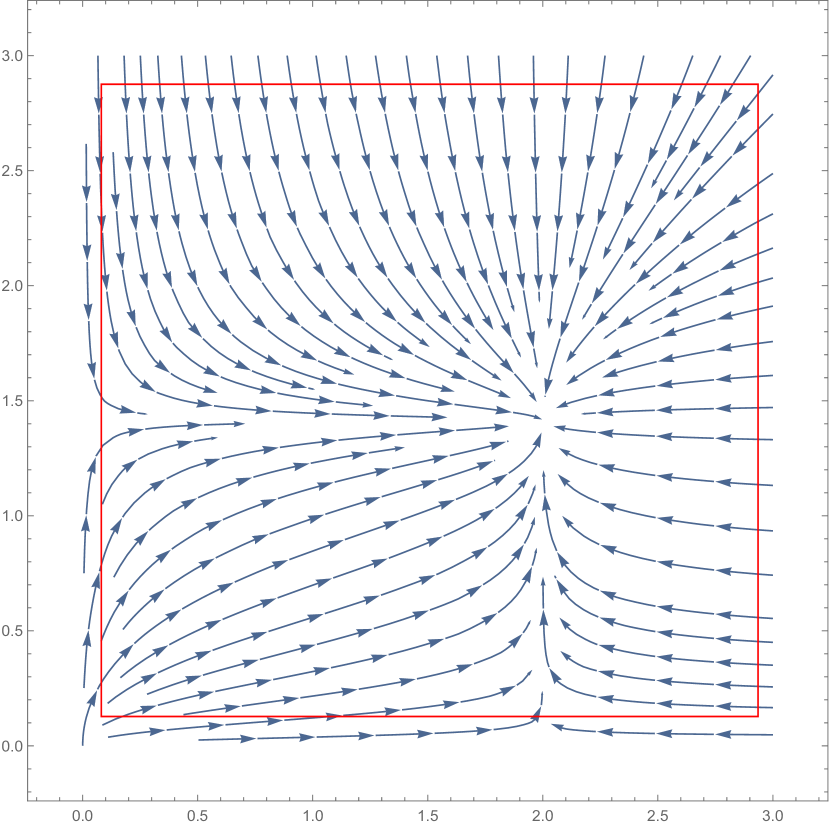
Figure 2: Flow of Negative Gradient

We will use Figures 2 and 2 to qualitatively establish the three steps in our framework.

1. From Figure 2, we note that $(2,\sqrt{2})$ is the global minimum. $(2,0),(0,\sqrt{2})$ are saddle points, while $(0,0)$ is local maximum. We notice all the stationary points which are not global minima lie on the surface $\sigma_{\min}(\mathbf{U})=0$, that is, the union of x-axis and y-axis.

2. By defining a boundary $\{\mathbf{U}|\sigma_{\min}(\mathbf{U})>c,\left\|{\mathbf{U}}\right\|_{2}<C\}$ for some small $c$ and large $C$ (corresponding to the red box in Figure 2), we see that negative gradient flow is pointed inside the box which means that for any point in the box, performing gradient descent with a small enough stepsize will ensure that all iterates lie inside the box (and hence keep away from saddle points).

3. Inside the red box, Figure 2 shows that negative gradient flow points to the global optimum. Moreover, we can indeed establish upper and lower bounds on the magnitude of gradients within the red box – this corresponds to establishing smoothness and gradient dominance respectively.

Together, all the above observations along with standard results in optimization tell us that gradient descent has geometric convergence for this problem.

We now present a formal proof of our result.

4.1 Location of Saddle Points

We first give a characterization of locations of all the stationary points which are not global minima.

Lemma 4.1.

Within symmetric PSD cone $\{\mathbf{U}|\mathbf{U}\succeq 0\}$, all stationary points of $f(\mathbf{U})=\left\|\mathbf{M}-\mathbf{U}^{2}\right\|_{F}^{2}$ which are not global minima, must satisfy $\sigma_{\min}\left(\mathbf{U}\right)=0$.

Proof.

For any stationary point $\mathbf{U}^{\prime}$ of $f(\mathbf{U})$ which is not on the boundary $\{\mathbf{U}|\sigma_{\min}(\mathbf{U})=0\}$, by linear algebra calculation, we have:

$$0= \|\nabla f(\mathbf{U}^{\prime})\|^{2}_{F}=\|(\mathbf{U}^{\prime 2}-\mathbf{M})\mathbf{U}^{\prime}+\mathbf{U}^{\prime}(\mathbf{U}^{\prime 2}-\mathbf{M})\|^{2}_{F}$$

$$= \langle(\mathbf{U}^{\prime 2}-\mathbf{M})\mathbf{U}^{\prime}+\mathbf{U}^{\prime}(\mathbf{U}^{\prime 2}-\mathbf{M}),$$

$$\quad\quad\quad\quad\quad\quad\quad(\mathbf{U}^{\prime 2}-\mathbf{M})\mathbf{U}^{\prime}+\mathbf{U}^{\prime}(\mathbf{U}^{\prime 2}-\mathbf{M})\rangle$$

$$= 2\text{Tr}([(\mathbf{U}^{\prime 2}-\mathbf{M})\mathbf{U}^{\prime}]^{2})+2\text{Tr}((\mathbf{U}^{\prime 2}-\mathbf{M})^{2}\mathbf{U}^{\prime 2})$$

$$\geq 4\sigma^{2}_{\min}(\mathbf{U}^{\prime})\|\mathbf{U}^{\prime 2}-\mathbf{M}\|_{F}^{2}$$

Therefore, since $\mathbf{U}^{\prime}$ is not on the boundary of PSD cone, we have $\sigma^{2}_{\min}(\mathbf{U})>0$, which gives $f(\mathbf{U}^{\prime})=\left\|\mathbf{M}-\mathbf{U}^{\prime 2}\right\|_{F}^{2}\neq 0$, thus $\mathbf{U}^{\prime}$ is global minima. ∎

As mentioned before, note that all the bad stationary points are contained in $\{\mathbf{U}|\sigma_{\min}\left(\mathbf{U}\right)=0\}$ which is a (Lebesgue) measure zero set.

4.2 Stay Away from Saddle Surface

Since the gradient at stationary points is zero, gradient descent can never converge to a global minimum if starting from suboptimal stationary points. Fortunately, in our case, gradient updates will keep away from bad stationary points. As in next Lemma, we show that as long as we choose suitable small learning rate, $\sigma_{\min}\left(\mathbf{U}_{t}\right)$ will never be too small.

Lemma 4.2.

Suppose $\eta<c\frac{\min\left(\sigma_{\min}\left(\mathbf{U_{0}}\right),\sigma^{1/2}_{\min}(\mathbf{M})/10\right)}{\max\left(\left\|{\mathbf{U_{0}}}\right\|_{2}^{3},\left(3\left\|{\mathbf{M}}\right\|_{2}\right)^{3/2}\right)}$, where $c$ is a small enough constant. Then, for every $t\in[T-1]$, we have $\mathbf{U_{t}}$ in Algorithm 1 be a PD matrix with

$$\lambda_{\min}\left(\mathbf{U_{t}}\right)\geq\min\left(\sigma_{\min}\left(\mathbf{U_{0}}\right),\frac{\sqrt{\sigma_{\min}\left(\mathbf{M}\right)}}{10}\right).$$

It turns out that the gradient updates will not only keep $\sigma_{\min}\left(\mathbf{U}\right)$ from being too small, but also keep $\left\|{\mathbf{U}}\right\|_{2}$ from being too large.

Lemma 4.3.

Suppose $\eta<\frac{1}{10\max\left(\left\|{\mathbf{U_{0}}}\right\|_{2}^{2},3{\left\|{\mathbf{M}}\right\|_{2}}\right)}$. For every $t\in[T-1]$, we have $\mathbf{U_{t}}$ in Algorithm 1 satisfying:

$$\left\|{\mathbf{U_{t}}}\right\|_{2}\leq\max\left(\left\|{\mathbf{U_{0}}}\right\|_{2},\sqrt{3\left\|{\mathbf{M}}\right\|_{2}}\right).$$

Although $\left\|{\mathbf{U}}\right\|_{2}$ is not directly related to the surface with bad stationary points, the upper bound on $\left\|{\mathbf{U}}\right\|_{2}$ is crucial for the smoothness of function $f(\cdot)$, which gives good convergence rate in Section 4.3.

4.3 Convergence in Saddle-Free Region

So far, we have been able to establish both upper bounds and lower bounds on singular values of all iterates $\mathbf{U}_{t}$ given suitable small learning rate. Next, we show that when spectral norm of $\mathbf{U}$ is small, function $f(\mathbf{U})$ is smooth, and when $\sigma_{\min}\left(\mathbf{U}\right)$ is large, function $f(\mathbf{U})$ is gradient dominated.

Lemma 4.4.

Function $f(\mathbf{U})=\left\|\mathbf{M}-\mathbf{U}^{2}\right\|_{F}^{2}$ is $8\max\{\Gamma,\left\|{\mathbf{M}}\right\|_{2}\}$-smooth in region $\{\mathbf{U}|\left\|{\mathbf{U}}\right\|_{2}^{2}\leq\Gamma\}$. That is, for any $\mathbf{U_{1}},\mathbf{U_{2}}\in\{\mathbf{U}|\left\|{\mathbf{U}}\right\|_{2}^{2}\leq\Gamma\}$, we have:

$$\|\nabla f(\mathbf{U_{1}})-\nabla f(\mathbf{U_{2}})\|_{F}\leq 8\max\{\Gamma,\left\|{\mathbf{M}}\right\|_{2}\}\|\mathbf{U_{1}}-\mathbf{U_{2}}\|_{F}$$

Lemma 4.5.

Function $f(\mathbf{U})=\left\|\mathbf{M}-\mathbf{U}^{2}\right\|_{F}^{2}$ is $4\gamma$-gradient dominated in region $\{\mathbf{U}|\sigma_{\min}\left(\mathbf{U}\right)^{2}\geq\gamma\}$. That is, for any $\mathbf{U}\in\{\mathbf{U}|\sigma_{\min}\left(\mathbf{U}\right)^{2}\geq\gamma\}$, we have:

$$\|\nabla f(\mathbf{U})\|^{2}_{F}\geq 4\gamma f(\mathbf{U})$$

Lemma 4.4 and 4.5 are the formal versions of Eq.(6) and Eq.(7) in Section 3.2, which are essential in establishing geometric convergence.

Putting all pieces together, we are now ready prove our main theorem:

Proof of Theorem 3.2.

Recall the definitions in Theorem 3.2:

$$\alpha \stackrel{{\scriptstyle\triangle}}{{=}}\left(\frac{\max\left(\left\|{\mathbf{U_{0}}}\right\|_{2},\sqrt{\left\|{\mathbf{M}}\right\|_{2}}\right)}{\min\left(\sigma_{\min}\left(\mathbf{U_{0}}\right),\sqrt{\sigma_{\min}\left(\mathbf{M}\right)}\right)}\right)^{3},$$

$$\beta \stackrel{{\scriptstyle\triangle}}{{=}}\min\left(\sigma_{\min}\left(\mathbf{U_{0}}\right),\sqrt{\sigma_{\min}\left(\mathbf{M}\right)}\right)$$

By choosing learning rate $\eta<\frac{c}{\alpha\beta^{2}}$ with small enough constant $c$. We can satisfy the precondition of Lemma 4.2, and Lemma 4.3 at same time. Therefore, we know all iterates will fall in region:

$$\left\{\mathbf{U}\left|\left\|{\mathbf{U}}\right\|_{2}\leq\max\left(\left\|{\mathbf{U_{0}}}\right\|_{2},\sqrt{3\left\|{\mathbf{M}}\right\|_{2}}\right)\right.\right.,$$

$$\quad\quad\left.\lambda_{\min}\left(\mathbf{U}\right)\geq\min\left(\sigma_{\min}\left(\mathbf{U_{0}}\right),\frac{\sqrt{\sigma_{\min}\left(\mathbf{M}\right)}}{10}\right)\right\}$$

Then, apply Lemma 4.4 and Lemma 4.5, we know in this region, function $f(\mathbf{U})=\left\|\mathbf{U}^{2}-\mathbf{M}\right\|_{F}^{2}$ has smoothness parameter:

$$8\max\left\{\max\left\{\left\|{\mathbf{U_{0}}}\right\|_{2}^{2},3\left\|{\mathbf{M}}\right\|_{2}\right\},\left\|{\mathbf{M}}\right\|_{2}\right\}\leq 24\alpha^{2/3}\beta^{2}$$

and gradient dominance parameter:

$$4\min\left\{\sigma_{\min}^{2}(\mathbf{U_{0}}),\frac{\sigma_{\min}\left(\mathbf{M}\right)}{100}\right\}\geq\frac{\beta^{2}}{25}$$

That is, $f(\mathbf{U})$ in the region is both $24\alpha^{2/3}\beta^{2}$-smooth, and $\beta^{2}/25$-gradient dominated.

Finally, by Taylor’s expansion of smooth function, we have:

$$f(\mathbf{U_{t+1}})\leq f(\mathbf{U_{t}})+\langle\nabla f(\mathbf{U_{t}}),\mathbf{U_{t+1}}-\mathbf{U_{t}}\rangle$$

$$\quad\quad\quad\quad\quad+12\alpha^{2/3}\beta^{2}\left\|\mathbf{U_{t+1}}-\mathbf{U_{t}}\right\|_{F}^{2}$$

$$= f(\mathbf{U_{t}})-(\eta-12\eta^{2}\alpha^{2/3}\beta^{2})\left\|\nabla f(\mathbf{U_{t}})\right\|_{F}^{2}$$

$$\leq f(\mathbf{U_{t}})-\frac{\eta}{2}\left\|\nabla f(\mathbf{U_{t}})\right\|_{F}^{2}$$

$$\leq (1-\eta\frac{\beta^{2}}{50})f(\mathbf{U_{t}})$$

The second last inequality is again by setting constant $c$ in learning rate to be small enough, and the last inequality is by the property of gradient dominated. This finishes the proof.

∎

5 Conclusion

In this paper, we take a first step towards addressing the large gap between local convergence results with good convergence rates and global convergence results with highly suboptimal convergence rates. We consider the problem of computing the squareroot of a PD matrix, which is a widely studied problem in numerical linear algebra, and show that non-convex gradient descent achieves global geometric convergence with a good rate. In addition, our analysis also establishes the stability of this method to numerical errors. We note that this is the first method to have provable robustness to numerical errors for this problem and our result illustrates that global convergence results are also useful in practice since they might shed light on the stability of optimization methods.

Our result shows that even in the presence of a large saddle point surface, gradient descent might be able to avoid it and converge to the global optimum at a linear rate. We believe that our framework and proof techniques should be applicable for several other nonconvex problems (especially those based on matrix factorization) in machine learning and numerical linear algebra and would lead to the analysis of gradient descent and stochastic gradient descent in a transparent way while also addressing key issues like robustness to noise or numerical errors.

Appendix A Proofs of Lemmas in Section 4

In this section, we restate the Lemmas in Section 4 which were used to prove Theorem 3.2, and present their proofs.

First, we prove lemmas which show a lower bound and a upper bound on the eigenvalues of the intermediate matrices $\mathbf{U_{t}}$ in Algorithm 1. This shows $\mathbf{U_{t}}$ always stay away from the surface where unwanted stationary point locate.

Lemma A.1 (Restatement of Lemma 4.2).

Suppose $\eta<\frac{c\min\left(\sigma_{\min}\left(\mathbf{U_{0}}\right),\sqrt{\sigma_{\min}\left(\mathbf{M}\right)}/10\right)}{\max\left(\left\|{\mathbf{U_{0}}}\right\|_{2}^{3},\left(3\left\|{\mathbf{M}}\right\|_{2}\right)^{3/2}\right)}$, where $c$ is a small enough constant. Then, for every $t\in[T-1]$, we have $\mathbf{U_{t}}$ be a PD matrix with

$$\lambda_{\min}\left(\mathbf{U_{t}}\right)\geq\min\left(\sigma_{\min}\left(\mathbf{U_{0}}\right),\frac{\sqrt{\sigma_{\min}\left(\mathbf{M}\right)}}{10}\right).$$

Proof.

We will prove the lemma by induction. The base case $t=0$ holds trivially. Suppose the lemma holds for some $t$. We will now prove that it holds for $t+1$. We have

$$\lambda_{\min}\left(\mathbf{U_{t+1}}\right)= \lambda_{\min}\left(\mathbf{U_{t}}-\eta\left(\mathbf{U_{t}}^{2}-\mathbf{M}\right)\mathbf{U_{t}}-\eta\mathbf{U_{t}}\left(\mathbf{U_{t}}^{2}-\mathbf{M}\right)\right)$$

$$\geq \lambda_{\min}\left(\frac{3}{4}\mathbf{U_{t}}-2\eta\mathbf{U_{t}}^{3}\right)+\lambda_{\min}\left(\frac{1}{4}\mathbf{U_{t}}+\eta(\mathbf{M}\mathbf{U_{t}}+\mathbf{U_{t}}\mathbf{M})\right)$$

$$= \lambda_{\min}\left(\frac{3}{4}\mathbf{U_{t}}-2\eta\mathbf{U_{t}}^{3}\right)+\lambda_{\min}\left(\left(\frac{1}{2}\mathbf{I}+\eta\mathbf{M}\right)\mathbf{U_{t}}\left(\frac{1}{2}\mathbf{I}+\eta\mathbf{M}\right)-\eta^{2}\mathbf{M}\mathbf{U_{t}}\mathbf{M}\right)$$ (8)

When $\eta\leq\frac{1}{100\max\left(\left\|{\mathbf{U_{0}}}\right\|_{2}^{2},3\left\|{\mathbf{M}}\right\|_{2}\right)}$, using Lemma 4.3 we can bound the first term as

$$\lambda_{\min}\left(\frac{3}{4}\mathbf{U_{t}}-2\eta\mathbf{U_{t}}^{3}\right)=\frac{3}{4}\sigma_{\min}\left(\mathbf{U_{t}}\right)-2\eta\sigma_{\min}\left(\mathbf{U_{t}}\right)^{3}.$$ (9)

To bound the second term, for any vector $\mathbf{w}\in\mathbb{R}^{n}$ with $\left\|{\mathbf{w}}\right\|_{2}=1$, let $\mathbf{w}=\sum_{i}^{n}\alpha_{i}\mathbf{v}_{i}$, where $\mathbf{v}_{i}$ is the $i^{\textrm{th}}$ eigenvector of $\mathbf{M}$, and $\sum_{i=1}^{n}\alpha_{i}^{2}=1$. Then:

$${\mathbf{w}}^{\top}\left(\left(\frac{1}{2}\mathbf{I}+\eta\mathbf{M}\right)\mathbf{U_{t}}\left(\frac{1}{2}\mathbf{I}+\eta\mathbf{M}\right)-\eta^{2}\mathbf{M}\mathbf{U_{t}}\mathbf{M}\right)\mathbf{w}$$

$$\geq \lambda_{\min}\left(\mathbf{U_{t}}\right)\left\|{\left(\frac{1}{2}\mathbf{I}+\eta\mathbf{M}\right)\mathbf{w}}\right\|_{2}^{2}-\eta^{2}\left\|{\mathbf{U_{t}}}\right\|_{2}\left\|{\mathbf{M}\mathbf{w}}\right\|_{2}^{2}$$

$$= \lambda_{\min}\left(\mathbf{U_{t}}\right)\sum_{i=1}^{n}\left(\frac{1}{2}+\eta\lambda_{i}\left(\mathbf{M}\right)\right)^{2}\alpha_{i}^{2}-\eta^{2}\left\|{\mathbf{U_{t}}}\right\|_{2}\sum_{i=1}^{n}\lambda_{i}\left(\mathbf{M}\right)^{2}\alpha_{i}^{2}$$

$$= \lambda_{\min}\left(\mathbf{U_{t}}\right)\sum_{i=1}^{n}\alpha_{i}^{2}\left(\frac{1}{4}+\eta\lambda_{i}\left(\mathbf{M}\right)+\eta^{2}\lambda_{i}\left(\mathbf{M}\right)^{2}-\eta^{2}\kappa\left(\mathbf{U_{t}}\right)\lambda_{i}\left(\mathbf{M}\right)^{2}\right)$$

$$\stackrel{{\scriptstyle(\zeta_{1})}}{{=}} \sigma_{\min}\left(\mathbf{U_{t}}\right)\sum_{i=1}^{n}\alpha_{i}^{2}\left(\frac{1}{4}+\eta\sigma_{i}\left(\mathbf{M}\right)+\eta^{2}\sigma_{i}\left(\mathbf{M}\right)^{2}-\eta^{2}\kappa\left(\mathbf{U_{t}}\right)\sigma_{i}\left(\mathbf{M}\right)^{2}\right)$$

$$\stackrel{{\scriptstyle(\zeta_{2})}}{{\geq}} \sigma_{\min}\left(\mathbf{U_{t}}\right)\sum_{i=1}^{n}\alpha_{i}^{2}\left(\frac{1}{4}+\frac{1}{2}\eta\sigma_{i}\left(\mathbf{M}\right)\right)\geq\sigma_{\min}\left(\mathbf{U_{t}}\right)\left(\frac{1}{4}+\frac{1}{2}\eta\sigma_{\min}\left(\mathbf{M}\right)\right),$$ (10)

where $(\zeta_{1})$ is due to the fact that $\mathbf{U_{t}}$ is a PD matrix, so $\lambda_{\min}\left(\mathbf{U_{t}}\right)=\sigma_{\min}\left(\mathbf{U_{t}}\right)\geq 0$, and $(\zeta_{2})$ is because since $\eta\leq\frac{\min\left(\sigma_{\min}\left(\mathbf{U_{0}}\right),\sqrt{\sigma_{\min}\left(\mathbf{M}\right)}/10\right)}{\max\left(\left\|{\mathbf{U_{0}}}\right\|_{2}^{3},\left(3\left\|{\mathbf{M}}\right\|_{2}\right)^{3/2}\right)}\leq\frac{1}{2\kappa\left(\mathbf{U_{t}}\right)\left\|{\mathbf{M}}\right\|_{2}}$, we have $\eta^{2}\kappa\left(\mathbf{U_{t}}\right)\sigma_{i}\left(\mathbf{M}\right)^{2}\leq\frac{1}{2}\eta\sigma_{i}\left(\mathbf{M}\right)$.

Plugging Eq.(9) and Eq.(10) into Eq.(8), we have:

$$\lambda_{\min}\left(\mathbf{U_{t+1}}\right)\geq\sigma_{\min}\left(\mathbf{U_{t}}\right)(1+\frac{1}{2}\eta\sigma_{\min}\left(\mathbf{M}\right)-2\eta\sigma_{\min}\left(\mathbf{U_{t}}\right)^{2})$$

When $\sigma_{\min}\left(\mathbf{U_{t}}\right)\leq\sqrt{\sigma_{\min}\left(\mathbf{M}\right)}/3$, we obtain:

$$\lambda_{\min}\left(\mathbf{U_{t+1}}\right)\geq\sigma_{\min}\left(\mathbf{U_{t}}\right)\geq\max\left(\sigma_{\min}\left(\mathbf{U_{0}}\right),\frac{\sqrt{\sigma_{\min}\left(\mathbf{M}\right)}}{10}\right),$$

and when $\sigma_{\min}\left(\mathbf{U_{t}}\right)\geq\sqrt{\sigma_{\min}\left(\mathbf{M}\right)}/3$, we have:

$$\lambda_{\min}\left(\mathbf{U_{t+1}}\right) \geq\sigma_{\min}\left(\mathbf{U_{t}}\right)(1-2\eta\sigma_{\min}\left(\mathbf{U_{t}}\right)^{2})$$

$$\geq\sigma_{\min}\left(\mathbf{U_{t}}\right)(1-2\eta\left\|{\mathbf{U_{t}}}\right\|_{2}^{2})\geq\frac{9}{10}\sigma_{\min}\left(\mathbf{U_{t}}\right)\geq\min\left(\sigma_{\min}\left(\mathbf{U_{0}}\right),\frac{\sqrt{\sigma_{\min}\left(\mathbf{M}\right)}}{10}\right).$$

This concludes the proof. ∎

Lemma A.2 (Restatement of Lemma 4.3).

Suppose $\eta<\frac{1}{10\max\left(\left\|{\mathbf{U_{0}}}\right\|_{2}^{2},3{\left\|{\mathbf{M}}\right\|_{2}}\right)}$. For every $t\in[T-1]$, we have:

$$\left\|{\mathbf{U_{t}}}\right\|_{2}\leq\max\left(\left\|{\mathbf{U_{0}}}\right\|_{2},\sqrt{3\left\|{\mathbf{M}}\right\|_{2}}\right).$$

Proof.

We will prove the lemma by induction. The base case $t=0$ is trivially true. Supposing the statement is true for $\mathbf{U_{t}}$, we will prove it for $\mathbf{U_{t+1}}$.

Using the update equation of Algorithm 1, we have:

$$\left\|{\mathbf{U_{t+1}}}\right\|_{2} =\left\|{\mathbf{U_{t}}-\eta\left(\mathbf{U_{t}}^{2}-\mathbf{M}\right)\mathbf{U_{t}}-\eta\mathbf{U_{t}}\left(\mathbf{U_{t}}^{2}-\mathbf{M}\right)}\right\|_{2}$$

$$=\left\|{\left(\mathbf{I}-2\eta\mathbf{U_{t}}^{2}\right)\mathbf{U_{t}}+\eta\mathbf{M}\mathbf{U_{t}}+\eta\mathbf{U_{t}}\mathbf{M}}\right\|_{2}$$

$$\leq\left\|{\left(\mathbf{I}-2\eta\mathbf{U_{t}}^{2}\right)\mathbf{U_{t}}}\right\|_{2}+2\eta\left\|{\mathbf{M}}\right\|_{2}\left\|{\mathbf{U_{t}}}\right\|_{2}.$$ (11)

The singular values of the matrix $\left(\mathbf{I}-2\eta\mathbf{U_{t}}^{2}\right)\mathbf{U_{t}}$ are exactly $(1-2\eta\sigma^{2})\cdot{\sigma}$ where $\sigma$ is a singular value of $\mathbf{U_{t}}$. For $\sigma\leq\sqrt{2\left\|{\mathbf{M}}\right\|_{2}}$, we clearly have $(1-2\eta\sigma^{2}){\sigma}\leq\sqrt{2\left\|{\mathbf{M}}\right\|_{2}}$. On the other hand, for $\sigma>\sqrt{2\left\|{\mathbf{M}}\right\|_{2}}$, we have $(1-2\eta\sigma^{2}){\sigma}<(1-4\eta\left\|{\mathbf{M}}\right\|_{2}){\sigma}$. Plugging this observation into Eq.(11), we obtain:

$$\left\|{\mathbf{U_{t+1}}}\right\|_{2} \leq\max\left(\sqrt{2\left\|{\mathbf{M}}\right\|_{2}},(1-4\eta\left\|{\mathbf{M}}\right\|_{2})\left\|{\mathbf{U_{t}}}\right\|_{2}\right)+2\eta\left\|{\mathbf{M}}\right\|_{2}\left\|{\mathbf{U_{t}}}\right\|_{2}$$

$$\leq\max\left(\sqrt{2\left\|{\mathbf{M}}\right\|_{2}}+\frac{1}{15}\left\|{\mathbf{U_{t}}}\right\|_{2},\left\|{\mathbf{U_{t}}}\right\|_{2}\right)\leq\max\left(\left\|{\mathbf{U_{0}}}\right\|_{2},\sqrt{3\left\|{\mathbf{M}}\right\|_{2}}\right),$$

where we used the inductive hypothesis in the last step. This proves the lemma. ∎

Finally, we prove the smoothness and gradient dominance in above regions.

Lemma A.3 (Restatement of Lemma 4.4).

For any $\mathbf{U_{1}},\mathbf{U_{2}}\in\{\mathbf{U}|\left\|{\mathbf{U}}\right\|_{2}^{2}\leq\Gamma\}$, we have function $f(\mathbf{U})=\left\|\mathbf{M}-\mathbf{U}^{2}\right\|_{F}^{2}$ satisfying:

$$\|\nabla f(\mathbf{U_{1}})-\nabla f(\mathbf{U_{2}})\|_{F}\leq 8\max\{\Gamma,\left\|{\mathbf{M}}\right\|_{2}\}\|\mathbf{U_{1}}-\mathbf{U_{2}}\|_{F}$$ (12)

Proof.

By expanding gradient $\nabla f(\mathbf{U})$, and reordering terms, we have:

$$\|\nabla f(\mathbf{U_{1}})-\nabla f(\mathbf{U_{2}})\|_{F}$$

$$= \|(2\mathbf{U_{1}}^{3}-\mathbf{M}\mathbf{U_{1}}-\mathbf{U_{1}}\mathbf{M})-(2\mathbf{U_{2}}^{3}-\mathbf{M}\mathbf{U_{2}}-\mathbf{U_{2}}\mathbf{M})\|_{F}$$

$$= \|2(\mathbf{U_{1}}^{3}-\mathbf{U_{2}}^{3})-\mathbf{M}(\mathbf{U_{1}}-\mathbf{U_{2}})-(\mathbf{U_{1}}-\mathbf{U_{2}})\mathbf{M}\|_{F}$$

$$\leq 2\|\mathbf{M}\|_{2}\|\mathbf{U_{1}}-\mathbf{U_{2}}\|_{F}+2\|\mathbf{U_{1}}^{3}-\mathbf{U_{2}}^{3}\|_{F}$$

$$= 2\|\mathbf{M}\|_{2}\|\mathbf{U_{1}}-\mathbf{U_{2}}\|_{F}+2\|\mathbf{U_{1}}^{2}(\mathbf{U_{1}}-\mathbf{U_{2}})+\mathbf{U_{1}}(\mathbf{U_{1}}-\mathbf{U_{2}})\mathbf{U_{2}}+(\mathbf{U_{1}}-\mathbf{U_{2}})\mathbf{U_{2}}^{2}\|_{F}$$

$$\leq 2\|\mathbf{M}\|_{2}\|\mathbf{U_{1}}-\mathbf{U_{2}}\|_{F}+6\Gamma\|\mathbf{U_{1}}-\mathbf{U_{2}}\|_{F}$$

$$\leq 8\max\{\Gamma,\left\|{\mathbf{M}}\right\|_{2}\}\|\mathbf{U_{1}}-\mathbf{U_{2}}\|_{F}$$

∎

Lemma A.4 (Restatement of Lemma 4.5).

For any $\mathbf{U}\in\{\mathbf{U}|\sigma_{\min}\left(\mathbf{U}\right)^{2}\geq\gamma\}$, we have function $f(\mathbf{U})=\left\|\mathbf{M}-\mathbf{U}^{2}\right\|_{F}^{2}$ satisfying:

$$\|\nabla f(\mathbf{U})\|^{2}_{F}\geq 4\gamma f(\mathbf{U})$$ (13)

Proof.

By expanding gradient $\nabla f(\mathbf{U})$, we have:

$$\|\nabla f(\mathbf{U})\|^{2}_{F}=\|(\mathbf{U}^{2}-\mathbf{M})\mathbf{U}+\mathbf{U}(\mathbf{U}^{2}-\mathbf{M})\|^{2}_{F}$$

$$= \langle(\mathbf{U}^{2}-\mathbf{M})\mathbf{U}+\mathbf{U}(\mathbf{U}^{2}-\mathbf{M}),(\mathbf{U}^{2}-\mathbf{M})\mathbf{U}+\mathbf{U}(\mathbf{U}^{2}-\mathbf{M})\rangle$$

$$\geq 4\sigma^{2}_{\min}(\mathbf{U})\|\mathbf{U}^{2}-\mathbf{M}\|_{F}^{2}=4\gamma f(\mathbf{U})$$

∎

Appendix B Proof of Theorem 3.4

In this section, we will prove Theorem 3.4. We first state a useful lemma which is a stronger version of Lemma 4.2

Lemma B.1.

Suppose $\mathbf{U_{t}}$ is a PD matrix with $\left\|{\mathbf{U_{t}}}\right\|_{2}\leq\max(\left\|{\mathbf{U_{0}}}\right\|_{2},\sqrt{3\left\|{\mathbf{M}}\right\|_{2}})$, and $\sigma_{\min}\left(\mathbf{U_{t}}\right)\geq\min(\sigma_{\min}\left(\mathbf{U_{0}}\right),\frac{1}{10}\sqrt{\sigma_{\min}\left(\mathbf{M}\right)})$. Suppose further that $\eta<\frac{c\min(\sigma_{\min}\left(\mathbf{U_{0}}\right),\frac{1}{10}\sqrt{\sigma_{\min}\left(\mathbf{M}\right)})}{\max(\left\|{\mathbf{U_{0}}}\right\|_{2},\sqrt{3\left\|{\mathbf{M}}\right\|_{2}})^{3/2}}$, where $c$ is a small enough constant and denote $\mathbf{U_{t+1}}\stackrel{{\scriptstyle\triangle}}{{=}}\mathbf{U_{t}}-\eta\left(\mathbf{U_{t}}^{2}-\mathbf{M}\right)\mathbf{U_{t}}-\eta\mathbf{U_{t}}\left(\mathbf{U_{t}}^{2}-\mathbf{M}\right)$. Then, $\mathbf{U_{t+1}}$ is a PD matrix with:

$$\lambda_{\min}\left(\mathbf{U_{t+1}}\right)\geq\left(1+\frac{\eta{\sigma_{\min}\left(\mathbf{M}\right)}}{15}\right)\min(\sigma_{\min}\left(\mathbf{U_{0}}\right),\frac{1}{10}\sqrt{\sigma_{\min}\left(\mathbf{M}\right)}).$$

Indeed, our proof of Lemma 4.2 already proves this stronger result. Now we are ready to prove Theorem 3.4.

Proof of Theorem 3.4.

The proof of the theorem is a fairly straight forward modification of the proof of Theorem 3.2. We will be terse since for most part we will use the arguments employed in the proofs of Theorem 3.2 and Lemmas 4.3 and 4.2.

We have the following two claims, which are robust versions of Lemmas 4.3 and 4.2, bounding the spectral norm and smallest eigenvalue of intermediate iterates. The proofs will be provided after the proof of the theorem.

Claim B.2.

For every $t\in[T-1]$, we have:

$$\left\|{\mathbf{U_{t}}}\right\|_{2}\leq\max(\left\|{\mathbf{U_{0}}}\right\|_{2},\sqrt{3\left\|{\mathbf{M}}\right\|_{2}}).$$

Claim B.3.

For every $t\in[T-1]$, we have $\mathbf{U_{t}}$ be a PD matrix with

$$\sigma_{\min}\left(\mathbf{U_{t}}\right)\geq\min(\sigma_{\min}\left(\mathbf{U_{0}}\right),\frac{\sqrt{\sigma_{\min}\left(\mathbf{M}\right)}}{10}).$$

We prove the theorem by induction. The base case $t=0$ holds trivially. Assuming the theorem is true for $t$, we will show it for $t+1$. Denoting $\mathbf{\widetilde{U}_{t+1}}\stackrel{{\scriptstyle\triangle}}{{=}}\mathbf{U_{t}}-\eta\left(\mathbf{U_{t}}^{2}-\mathbf{M}\right)\mathbf{U_{t}}-\eta\mathbf{U_{t}}\left(\mathbf{U_{t}}^{2}-\mathbf{M}\right)$, we have

$$\left\|\mathbf{M}-\mathbf{U_{t+1}}^{2}\right\|_{F} =\left\|\mathbf{M}-\mathbf{\widetilde{U}_{t+1}}^{2}-\mathbf{\widetilde{U}_{t+1}}\mathbf{\bigtriangleup_{t}}-\mathbf{\bigtriangleup_{t}}\mathbf{\widetilde{U}_{t+1}}-\mathbf{\bigtriangleup_{t}}^{2}\right\|_{F}$$

$$\leq\left\|\mathbf{M}-\mathbf{\widetilde{U}_{t+1}}^{2}\right\|_{F}+2\left\|{\mathbf{\widetilde{U}_{t+1}}}\right\|_{2}\left\|\mathbf{\bigtriangleup_{t}}\right\|_{F}+\left\|\mathbf{\bigtriangleup_{t}}^{2}\right\|_{F}.$$ (14)

Using Claims B.2 and B.3, Lemma 4.3 tells us that

$$\left\|{\mathbf{\widetilde{U}_{t+1}}}\right\|_{2}\leq\max(\left\|{\mathbf{U_{0}}}\right\|_{2},\sqrt{3\left\|{\mathbf{M}}\right\|_{2}}),$$

and Theorem 3.2 tells us that

$$\left\|\mathbf{M}-\mathbf{\widetilde{U}_{t+1}}^{2}\right\|_{F}\leq\exp\left(-\widehat{c}\eta\min(\sigma_{\min}\left(\mathbf{U_{0}}\right)^{2},\sigma_{\min}\left(\mathbf{M}\right))\right)\left\|\mathbf{M}-\mathbf{U_{t}}^{2}\right\|_{F}.$$

Plugging the above two conclusions into (14), tells us that

$$\left\|\mathbf{M}-\mathbf{U_{t+1}}^{2}\right\|_{F}$$

$$\leq\exp\left(-\widehat{c}\eta\min(\sigma_{\min}\left(\mathbf{U_{0}}\right)^{2},\sigma_{\min}\left(\mathbf{M}\right))\right)\left\|\mathbf{M}-\mathbf{U_{t}}^{2}\right\|_{F}+2\max(\left\|{\mathbf{U_{0}}}\right\|_{2},\sqrt{3\left\|{\mathbf{M}}\right\|_{2}})\left\|\mathbf{\bigtriangleup_{t}}\right\|_{F}$$

$$\qquad+\frac{1}{30}\eta\sigma_{\min}\left(\mathbf{M}\right)\min(\sigma_{\min}\left(\mathbf{U_{0}}\right),\sqrt{\sigma_{\min}\left(\mathbf{M}\right)})\left\|\mathbf{\bigtriangleup_{t}}\right\|_{F}$$

$$\leq\exp\left(-\widehat{c}\eta\min(\sigma_{\min}\left(\mathbf{U_{0}}\right)^{2},\sigma_{\min}\left(\mathbf{M}\right))\right)\left\|\mathbf{M}-\mathbf{U_{0}}^{2}\right\|_{F}$$

$$\qquad+4\max(\left\|{\mathbf{U_{0}}}\right\|_{2},\sqrt{3\left\|{\mathbf{M}}\right\|_{2}})\sum_{s=0}^{t}\exp\left(-\widehat{c}\eta\min(\sigma_{\min}\left(\mathbf{U_{0}}\right)^{2},\sigma_{\min}\left(\mathbf{M}\right))(t-s)\right)\left\|\mathbf{\bigtriangleup_{s}}\right\|_{F},$$

where we used the induction hypothesis in the last step. ∎

We now prove Claim B.2.

Proof of Claim B.2.

Just as in the proof of Lemma 4.3, we will use induction. Assuming the claim is true for $\mathbf{U_{t}}$, by update equation

$$\mathbf{U_{t+1}}=\mathbf{U_{t}}-\eta\left(\mathbf{U_{t}}^{2}-\mathbf{M}\right)\mathbf{U_{t}}-\eta\mathbf{U_{t}}\left(\mathbf{U_{t}}^{2}-\mathbf{M}\right)+\mathbf{\bigtriangleup_{t}}$$

We can write out:

$$\left\|{\mathbf{U_{t+1}}}\right\|_{2} \leq\left\|{\left(\mathbf{I}-2\eta\mathbf{U_{t}}^{2}\right)\mathbf{U_{t}}}\right\|_{2}+\eta\left\|{\mathbf{M}}\right\|_{2}\left\|{\mathbf{U_{t}}}\right\|_{2}+\eta\left\|{\mathbf{U_{t}}}\right\|_{2}\left\|{\mathbf{M}}\right\|_{2}+\left\|{\mathbf{\bigtriangleup_{t}}}\right\|_{2}.$$ (15)

Since $\eta<\frac{1}{10\max(\left\|{\mathbf{U_{0}}}\right\|_{2}^{2},\left\|{\mathbf{M}}\right\|_{2})}$ and $\left\|{\mathbf{U_{t}}}\right\|_{2}\leq\max(\left\|{\mathbf{U_{0}}}\right\|_{2},\sqrt{3\left\|{\mathbf{M}}\right\|_{2}})$, note that the singular values of the matrix $\left(\mathbf{I}-2\eta\mathbf{U_{t}}^{2}\right)\mathbf{U_{t}}$ are exactly $(1-2\eta\sigma^{2})\cdot{\sigma}$ where $\sigma$ is a singular value of $\mathbf{U_{t}}$. For $\sigma\leq\sqrt{2\left\|{\mathbf{M}}\right\|_{2}}$, we clearly have $(1-2\eta\sigma^{2}){\sigma}\leq\sqrt{2\left\|{\mathbf{M}}\right\|_{2}}$. On the other hand, for $\sigma>\sqrt{2\left\|{\mathbf{M}}\right\|_{2}}$, we have $(1-2\eta\sigma^{2}){\sigma}<(1-4\eta\left\|{\mathbf{M}}\right\|_{2}){\sigma}$. Plugging this observation into (15), we obtain:

$$\left\|{\mathbf{U_{t+1}}}\right\|_{2} \leq\max\left(\sqrt{2\left\|{\mathbf{M}}\right\|_{2}},(1-4\eta\left\|{\mathbf{M}}\right\|_{2})\left\|{\mathbf{U_{t}}}\right\|_{2}\right)+2\eta\left\|{\mathbf{M}}\right\|_{2}\left\|{\mathbf{U_{t}}}\right\|_{2}+\left\|{\mathbf{\bigtriangleup_{t}}}\right\|_{2}$$

$$\leq\max(\left\|{\mathbf{U_{0}}}\right\|_{2},\sqrt{3\left\|{\mathbf{M}}\right\|_{2}}),$$

proving the claim. ∎

We now prove Claim B.3.

Proof of Claim B.3.

We will use induction, with the proof following fairly easily using Lemma B.1. Suppose $\sigma_{\min}\left(\mathbf{U_{t}}\right)\geq\min(\sigma_{\min}\left(\mathbf{U_{0}}\right),\frac{1}{10}\sqrt{\sigma_{\min}\left(\mathbf{M}\right)})$. Denoting

$$\mathbf{\widetilde{U}_{t+1}}\stackrel{{\scriptstyle\triangle}}{{=}}\mathbf{U_{t}}-\eta\left(\mathbf{U_{t}}^{2}-\mathbf{M}\right)\mathbf{U_{t}}-\eta\mathbf{U_{t}}\left(\mathbf{U_{t}}^{2}-\mathbf{M}\right),$$

Lemma B.1 tells us that

$$\sigma_{\min}\left(\mathbf{\widetilde{U}_{t+1}}\right)\geq\left(1+\frac{\eta{\sigma_{\min}\left(\mathbf{M}\right)}}{15}\right)\min(\sigma_{\min}\left(\mathbf{U_{0}}\right),\frac{1}{10}\sqrt{\sigma_{\min}\left(\mathbf{M}\right)}),$$

which then implies the claim, since

$$\sigma_{\min}\left(\mathbf{U_{t+1}}\right)\geq\sigma_{\min}\left(\mathbf{U_{t+1}}\right)-\left\|{\mathbf{\bigtriangleup_{t}}}\right\|_{2}\geq\min(\sigma_{\min}\left(\mathbf{U_{0}}\right),\frac{1}{10}\sqrt{\sigma_{\min}\left(\mathbf{M}\right)}).$$

∎

Appendix C Proof of Theorem 3.5

In this section, we will prove Theorem 3.5.

Proof.

Consider two-dimensional case, where

$$\mathbf{M}=\begin{pmatrix}\left\|{\mathbf{M}}\right\|_{2}&0\\ 0&\sigma_{\min}\left(\mathbf{M}\right)\end{pmatrix}$$

We will prove Theorem 3.5 by considering two cases of step size (where $\eta\geq\frac{1}{4\left\|{\mathbf{M}}\right\|_{2}}$ or $\eta<\frac{1}{4\left\|{\mathbf{M}}\right\|_{2}}$) separately.

Case 1

: For step size $\eta\geq\frac{1}{4\left\|{\mathbf{M}}\right\|_{2}}$. Let $\beta=\frac{1}{2\eta\left\|{\mathbf{M}}\right\|_{2}}+1$, and consider following initialization $\mathbf{U_{0}}$:

$$\mathbf{U_{0}}=\begin{pmatrix}\sqrt{\beta\left\|{\mathbf{M}}\right\|_{2}}&0\\ 0&\sqrt{\sigma_{\min}\left(\mathbf{M}\right)}\end{pmatrix}$$

Since $\eta\geq\frac{1}{4\left\|{\mathbf{M}}\right\|_{2}}$, we know $\beta\leq 3$, which satisfies our assumption about $\mathbf{U_{0}}$ and $\mathbf{M}$. By calculation, we have:

$$\mathbf{U_{0}}(\mathbf{U_{0}}^{2}-\mathbf{M})+(\mathbf{U_{0}}^{2}-\mathbf{M})\mathbf{U_{0}}=\begin{pmatrix}2(\beta-1)\sqrt{\beta\left\|{\mathbf{M}}\right\|_{2}^{3}}&0\\ 0&0\end{pmatrix}$$

and since $2\eta(\beta-1)\left\|{\mathbf{M}}\right\|_{2}=1$, we have:

$$\mathbf{U_{1}}=\mathbf{U_{0}}-\eta[\mathbf{U_{0}}(\mathbf{U_{0}}^{2}-\mathbf{M})+(\mathbf{U_{0}}^{2}-\mathbf{M})\mathbf{U_{0}}]=\begin{pmatrix}\sqrt{\beta\left\|{\mathbf{M}}\right\|_{2}}-2\eta(\beta-1)\sqrt{\beta\left\|{\mathbf{M}}\right\|_{2}^{3}}&0\\ 0&1\end{pmatrix}=\begin{pmatrix}0&0\\ 0&1\end{pmatrix}$$

Then, by induction we can easily show for all $t\geq 1$, $\mathbf{U_{t}}=\mathbf{U_{1}}$, thus $\left\|\mathbf{U_{t}}^{2}-\mathbf{M}\right\|_{F}\geq\left\|{\mathbf{M}}\right\|_{2}\geq\frac{1}{4}\sigma_{\min}\left(\mathbf{M}\right)$ .

Case 2

: For step size $\eta\leq\frac{1}{4\left\|{\mathbf{M}}\right\|_{2}}$, consider following initialization $\mathbf{U_{0}}$:

$$\mathbf{U_{0}}=\begin{pmatrix}\sqrt{\left\|{\mathbf{M}}\right\|_{2}}&0\\ 0&\frac{1}{2}\sqrt{\sigma_{\min}\left(\mathbf{M}\right)}\end{pmatrix}$$

According to the update rule in Algorithm 1, we can easily show by induction that: for any $t\geq 0$, $\mathbf{U_{t}}$ is of form:

$$\mathbf{U_{t}}=\begin{pmatrix}\sqrt{\left\|{\mathbf{M}}\right\|_{2}}&0\\ 0&\alpha_{t}\sqrt{\sigma_{\min}\left(\mathbf{M}\right)}\end{pmatrix}$$

where $\alpha_{t}$ is a factor that depends on $t$, satisfying $0\leq\alpha_{t}\leq 1$ and:

$$\alpha_{t+1}=\alpha_{t}[1+\eta\sigma_{\min}\left(\mathbf{M}\right)(1-\alpha_{t}^{2})],\quad\alpha_{0}=\frac{1}{2}$$

Since $\eta\leq\frac{1}{4\left\|{\mathbf{M}}\right\|_{2}}$, we know:

$$\alpha_{t+1}\leq\alpha_{t}[1+\frac{1}{4\kappa}(1-\alpha_{t}^{2})]\leq\alpha_{t}+\frac{1}{4\kappa}$$

Therefore, for all $t\leq\kappa$, we have $\alpha_{t}\leq\frac{3}{4}$, and thus $\left\|\mathbf{U_{t}}^{2}-\mathbf{M}\right\|_{F}\geq\frac{1}{4}\sigma_{\min}\left(\mathbf{M}\right)$. ∎

References

- Agarwal et al. [2013] Alekh Agarwal, Animashree Anandkumar, Prateek Jain, and Praneeth Netrapalli. Learning sparsely used overcomplete dictionaries via alternating minimization. arXiv preprint, 2013.
- Aharon et al. [2006] Michal Aharon, Michael Elad, and Alfred Bruckstein. K-SVD: An algorithm for designing overcomplete dictionaries for sparse representation. Signal Processing, IEEE Transactions on, 54(11):4311–4322, 2006.
- Björck and Hammarling [1983] Åke Björck and Sven Hammarling. A Schur method for the square root of a matrix. Linear algebra and its applications, 52:127–140, 1983.
- Candes et al. [2015] Emmanuel J Candes, Xiaodong Li, and Mahdi Soltanolkotabi. Phase retrieval via wirtinger flow: Theory and algorithms. Information Theory, IEEE Transactions on, 61(4):1985–2007, 2015.
- Carlson [1990] Neal Carlson. Federated square root filter for decentralized parallel processors. Aerospace and Electronic Systems, IEEE Transactions on, 26(3):517–525, 1990.
- Ge et al. [2015] Rong Ge, Furong Huang, Chi Jin, and Yang Yuan. Escaping from saddle points—online stochastic gradient for tensor decomposition. In Proceedings of The 28th Conference on Learning Theory, pages 797–842, 2015.
- Golub and Van Loan [2012] Gene H Golub and Charles F Van Loan. Matrix computations, volume 3. JHU Press, 2012.
- Higham [1986] Nicholas J Higham. Newton’s method for the matrix square root. Mathematics of Computation, 46(174):537–549, 1986.
- Higham [1987] Nicholas J Higham. Computing real square roots of a real matrix. Linear Algebra and its applications, 88:405–430, 1987.
- Higham [1997] Nicholas J Higham. Stable iterations for the matrix square root. Numerical Algorithms, 15(2):227–242, 1997.
- Higham [2008] Nicholas J Higham. Functions of matrices: theory and computation. Society for Industrial and Applied Mathematics (SIAM), 2008.
- Jain and Netrapalli [2014] Prateek Jain and Praneeth Netrapalli. Fast exact matrix completion with finite samples. arXiv preprint, 2014.
- Jain et al. [2013] Prateek Jain, Praneeth Netrapalli, and Sujay Sanghavi. Low-rank matrix completion using alternating minimization. In Proceedings of the forty-fifth annual ACM symposium on Theory of computing, pages 665–674. ACM, 2013.
- Jin et al. [2017] Chi Jin, Rong Ge, Praneeth Netrapalli, Sham M Kakade, and Michael I Jordan. How to escape saddle points efficiently. arXiv preprint arXiv:1703.00887, 2017.
- Kaminski et al. [1971] Paul G Kaminski, Arthur E Bryson Jr, and Stanley F Schmidt. Discrete square root filtering: A survey of current techniques. Automatic Control, IEEE Transactions on, 16(6):727–736, 1971.
- Koren et al. [2009] Yehuda Koren, Robert Bell, and Chris Volinsky. Matrix factorization techniques for recommender systems. Computer, (8):30–37, 2009.
- Lee and Seung [2001] Daniel D Lee and H Sebastian Seung. Algorithms for non-negative matrix factorization. In Advances in neural information processing systems, pages 556–562, 2001.
- Lee et al. [2016] Jason D Lee, Max Simchowitz, Michael I Jordan, and Benjamin Recht. Gradient descent converges to minimizers. University of California, Berkeley, 1050:16, 2016.
- Meini [2004] Beatrice Meini. The matrix square root from a new functional perspective: theoretical results and computational issues. SIAM journal on matrix analysis and applications, 26(2):362–376, 2004.
- Musco and Musco [2015] Cameron Musco and Christopher Musco. Stronger approximate singular value decomposition via the block lanczos and power methods. arXiv preprint, 2015.
- Nesterov and Polyak [2006] Yurii Nesterov and Boris T Polyak. Cubic regularization of newton method and its global performance. Mathematical Programming, 108(1):177–205, 2006.
- Netrapalli et al. [2015] Praneeth Netrapalli, Prateek Jain, and Sujay Sanghavi. Phase retrieval using alternating minimization. IEEE Transactions on Signal Processing, 63(18):4814–4826, 2015.
- Pan et al. [1998] Victor Y Pan, Zhao Q Chen, and Ailong Zheng. The complexity of the algebraic eigenproblem. Mathematical Sciences Research Institute, Berkeley, page 71, 1998.
- Polyak [1963] BT Polyak. Gradient methods for the minimisation of functionals. USSR Computational Mathematics and Mathematical Physics, 3(4):864–878, 1963.
- Recht et al. [2010] Benjamin Recht, Maryam Fazel, and Pablo A Parrilo. Guaranteed minimum-rank solutions of linear matrix equations via nuclear norm minimization. SIAM review, 52(3):471–501, 2010.
- Sra [2015] Suvrit Sra. On the matrix square root via geometric optimization. arXiv preprint, 2015.
- Sun et al. [2015] Ju Sun, Qing Qu, and John Wright. When are nonconvex problems not scary? arXiv preprint arXiv:1510.06096, 2015.
- Sun and Luo [2015] Ruoyu Sun and Zhi-Quan Luo. Guaranteed matrix completion via nonconvex factorization. In Foundations of Computer Science (FOCS), 2015 IEEE 56th Annual Symposium on, pages 270–289. IEEE, 2015.
- Tippett et al. [2003] Michael K Tippett, Jeffrey L Anderson, Craig H Bishop, Thomas M Hamill, and Jeffrey S Whitaker. Ensemble square root filters*. Monthly Weather Review, 131(7):1485–1490, 2003.
- Tu et al. [2015] Stephen Tu, Ross Boczar, Mahdi Soltanolkotabi, and Benjamin Recht. Low-rank solutions of linear matrix equations via procrustes flow. arXiv preprint arXiv:1507.03566, 2015.
- Van Der Merwe and Wan [2001] Ronell Van Der Merwe and Eric Wan. The square-root unscented kalman filter for state and parameter-estimation. In Acoustics, Speech, and Signal Processing, 2001. Proceedings.(ICASSP’01). 2001 IEEE International Conference on, volume 6, pages 3461–3464. IEEE, 2001.
- Williams [2012] Virginia Vassilevska Williams. Multiplying matrices faster than coppersmith-winograd. In Proceedings of the forty-fourth annual ACM symposium on Theory of computing, pages 887–898. ACM, 2012.