Correlations between bulk parameters in relativistic and nonrelativistic hadronic mean-field models.

Abstract

In this work, we study the arising of correlations among some isoscalar ($K_{o}$, $Q_{o}$, and $I_{o}$) and isovector ($J$, $L_{o}$, $K_{\mbox{\tiny sym}}^{o}$, $Q_{\mbox{\tiny sym}}^{o}$, and $I_{\mbox{\tiny sym}}^{o}$) bulk parameters in nonrelativistic and relativistic hadronic mean-field models. For the former, we investigate correlations in Skyrme and Gogny parametrizations, as well as in the nonrelativistic (NR) limit of relativistic point-coupling models. We provide analytical correlations among bulk parameters for the NR limit, discussing the conditions in which they are linear ones. Based on a recent study [B. M. Santos et al., Phys. Rev. C 90, 035203 (2014)], we also show that some correlations presented in the NR limit are reproduced for relativistic models presenting cubic and quartic self-interactions in the scalar field $\sigma$, mostly studied in this work in the context of the relativistic framework. We also discuss how the crossing points, observed in the density dependence of some bulk parameters, can be seen as a signature of linear correlations between the specific bulk quantity presenting the crossing, and its immediately next order parameter.

I Introduction

In a general way, there are at least two different and competitive approaches in the treatment of nuclear matter. One of them is based on nucleon-nucleon interactions, from which many-nucleon microscopic relativistic/nonrelativistic Brueckner-Hartree-Fock (BHF) bhf calculations are performed to obtain information regarding the entire nuclear system. These calculations depend on the chosen nucleon-nucleon potential, classified as phenomenological (Reid, Urbana and Argonne interactions, for instance) or theoretical one-boson exchange ones (Paris, Bonn and Nijmegen interactions, for instance). For a short review, see Ref. rpot . Such nucleon-nucleon interactions reproduce experimental data on phase-shifts and deuteron properties and are implemented in complicated many-nucleon BHF codes in order to obtain nuclear matter properties. Alternatively, a second (macroscopic) approach does not use nucleon-nucleon interaction itself. This is the case of nonrelativistic mean-field models like Skyrme skyrme and Gogny gog ones. In relativistic framework, on the other hand, the most used models are the relativistic mean-field (RMF) Walecka model walecka , and its improved versions rmf .

In both approaches, many of the models and approximations used are intrinsically related to the fact that an analytical expression for the nucleon-nucleon potential is unknown. Therefore, in a theoretical point of view, correlations between two or more observables acquire enormous importance due to the fact that they reduce the set of independent relevant quantities to be used in the construction of nuclear models, avoiding redundant free-parameter fittings. In an experimental point of view, on the other hand, a correlation between two observables $\mathcal{A}$ and $\mathcal{B}$, for instance, allows the complete knowledge of $\mathcal{B}$ if $\mathcal{A}$ is experimentally well constrained.

In the few-body nuclear physics, for example, the Tjon line tjon , establishes a correlation between the binding energies of ${}^{4}\rm He$ and triton, $B_{\alpha}$ and $B_{t}$, respectively. The parametrization of the numerical results for several two-nucleon potentials plb concludes that such a correlation reads roughly $B_{\alpha}=4.72(B_{t}-2.48)$, in MeV units. It means that, if $B_{t}$ is calculated by using a two nucleon-nucleon potential, the value of $B_{\alpha}$ is predicted, even before any four-nucleon calculation.

Concerning correlations among bulk parameters, there are still a few of them well established in the literature. One of them, usually known as the Coester line coester , correlates the saturation density $\rho_{o}$ and the nuclear matter binding energy $B_{o}$. It was analyzed in Ref. coester in a two-nucleon model interaction, by varying its tensor force contribution while keeping the deuteron binding energy fixed. They showed that the function $B_{o}\times\rho_{o}$ roughly follows a line, in fact a band, also observing its similarity with the curve constructed from $B_{o}$ and $\rho_{o}$ obtained from distinct two-nucleon potentials. Even modern calculations using Brueckner-Hartree-Fock, and including single-particle contribution in the continuum, change the results but preserve the Coester line. Another correlation was studied in Ref. ls-splitting , and involves the relationship between finite nuclei spin-orbit splittings and the ratio $m^{*}=M^{*}_{o}/M$ for a class of finite-range (FR) RMF models, being $M^{*}_{o}$ the nucleon Dirac effective mass at $\rho=\rho_{o}$ and $M$ the nucleon rest mass. The authors showed that such splittings are experimentally well reproduced if the range for $m^{*}$ is constrained to the following inequality,

$$0.58\leqslant m^{*}\leqslant 0.64.$$ (1)

We will refer the above relation extracted from Ref. ls-splitting as the FRS constraint. It is important because it relates bulk infinite nuclear matter calculation with the closed shell finite nuclei energy spectrum. Still regarding relationships among quantities of finite nuclei and infinite nuclear matter, we also point out the correlation between the neutron skin thickness in ${}^{208}\rm Pb$, and the liquid-to-solid transition density in neutron-rich matter, investigated in Ref. skin with RMF models.

In a recent paper bianca , we have provided analytical expressions linearly correlating the symmetry energy ($J$), its slope ($L_{o}$) and curvature ($K_{\mbox{\tiny sym}}^{o}$) at the saturation density in the framework of the nonrelativistic (NR) limit of nonlinear point-coupling (NLPC) versions of the Boguta-Bodmer models boguta (FR-RMF models presenting cubic and quartic self-interactions in the scalar field $\sigma$). From such analytical correlations, we were able to predict ranges for $L_{o}$ that Boguta-Bodmer models must present in order furnish good values for finite nuclei spin-orbit splittings. In this paper, we further investigate the arising of correlations among bulk parameters of infinite nuclear matter at zero temperature in nonrelativistic and relativistic hadronic mean-field models. For the former, we choose some Skyrme and Gogny parametrizations as well as the NR limit of NLPC models. For the latter, we choose FR-RMF models, specially the Boguta-Bodmer ones, and show the conditions to be satisfied in order to their bulk parameters present correlations. In particular, we show, in a general way, how linear correlations are connected with crossing points in the density dependence of bulk parameters. For this purpose, we generalize the procedure used in Ref. margueron , where the authors associated the crossing point in the incompressibility function for different nonrelativistic Skyrme models, but not for FR-RMF ones, with the linear correlation between $K_{o}$ and $Q_{o}$ (incompressibility and skewness coefficient at $\rho_{o}$, respectively). We show here that there are other crossing densities different from $\rho_{c}\simeq 0.7\rho_{o}$, value found in Refs. margueron ; prl , for different bulk parameters in nonrelativistic models, as well as in relativistic ones. In the following, we will see that such crossing densities may be seen as signatures of linear correlations between higher order derivatives of the specific bulk parameter presenting the crossing.

The paper is organized as follows. In Sec. II we show how linear correlations are connected with crossing densities in bulk parameters of infinite nuclear matter. In Sec. III, we use some results of our previous study of the NR limit bianca , in order to apply the calculations of the previous section. In Sec. IV, we use the predictions of the NR limit to study the conditions that establish linear correlations in FR-RMF models. In Sec. V, we study relativistic and nonrelativistic models presenting two isovector coupling constants in the context of the correlation between the symmetry energy and its slope. Finally, we present our main conclusions in Sec. VI.

II Connection between linear correlations and crossing densities

In the literature, it is verified that crossing points can occur in the density dependence of the symmetry energy 19 , in pure neutron matter equation of state 20 , and in pairing gap of nuclear matter 22 , for instance. Recently, in Refs. prl ; margueron , the authors found a specific crossing point in the incompressibility of nuclear matter for different nonrelativistic Skyrme models, and not confirmed in FR-RMF ones. They showed that this crossing density ($\rho_{c}\simeq 0.7\rho_{o}\simeq 0.11$ fm^-3) when used in the calculation of the derivative of the incompressibility, makes this quantity better correlated to the centroid energy of the isoscalar giant monopole resonance than $K_{o}$. The authors also pointed out that this crossing density $\rho_{c}$ is closer to the average density in the ${}^{208}{\rm Pb}$ nucleus, $\langle\rho\rangle=0.12$ fm^-3, than the saturation density itself, $\rho_{o}\simeq 0.16$ fm^-3, with $\langle\rho\rangle$ also obtained by using the Skyrme model. The question we pose here is what properly mean, or indicate, such crossing points. In the following, we try to answer this question.

Actually, crossing points in different bulk parameters of infinity nuclear matter can be viewed as a signature of linear correlations between higher order derivatives of that particular bulk parameter presenting the crossing in its density dependence. In order to make it clear, we proceed to generalize the calculation performed in Ref. margueron , where the authors associated a crossing in the $K(\rho)$ function with the linear correlation between $K_{o}$ and $Q_{o}$ for some Skyrme parametrizations. Firstly, let us define a function of the density, $\mathcal{F}(\rho)$, expanded in terms of the dimensionless variable $x=\frac{\rho-\rho_{o}}{3\rho_{o}}$, and around the saturation density as,

$$\mathcal{F}(\rho)=\mathcal{F}(\rho_{o})+\mathcal{F}^{\prime}(\rho_{o})x+\frac{\mathcal{F}^{\prime\prime}(\rho_{o})}{2!}x^{2}+\frac{\mathcal{F}^{\prime\prime\prime}(\rho_{o})}{3!}x^{3}+\cdots$$ (2)

with the derivatives of $\mathcal{F}(\rho)$ given by

$$\mathcal{F}^{(m)}(\rho)=(3\rho)^{m}\frac{\partial}{\partial\rho}\left[\frac{\mathcal{F}^{(m-1)}(\rho)}{(3\rho)^{m-1}}\right],$$ (3)

for $m=1,2,3\,...$

For the values $m=1,2,3$, for instance, and by noting that $\frac{\rho}{\rho_{o}}=3x+1$ and $\frac{\partial}{\partial\rho}=\frac{\partial x}{\partial\rho}\frac{\partial}{\partial x}=\frac{1}{3\rho_{o}}\frac{\partial}{\partial x}$, we see that Eq. (3) leads to

$$\mathcal{F}^{\prime}(\rho) = 3\rho\frac{\partial\mathcal{F}}{\partial\rho}=\frac{3\rho}{3\rho_{o}}\frac{\partial\mathcal{F}}{\partial x}=(3x+1)\frac{\partial\mathcal{F}}{\partial x},$$ (4)

$$\mathcal{F}^{\prime\prime}(\rho) = (3\rho)^{2}\frac{\partial}{\partial\rho}\left[\frac{\mathcal{F}^{\prime}(\rho)}{3\rho}\right]=(3\rho)^{2}\frac{\partial}{\partial\rho}\left[\frac{\partial\mathcal{F}}{\partial\rho}\right]$$ (5)

$$= \frac{(3\rho)^{2}}{(3\rho_{o})^{2}}\frac{\partial^{2}\mathcal{F}}{\partial x^{2}}=(3x+1)^{2}\frac{\partial^{2}\mathcal{F}}{\partial x^{2}},$$

and

$$\mathcal{F}^{\prime\prime\prime}(\rho) = (3\rho)^{3}\frac{\partial}{\partial\rho}\left[\frac{\mathcal{F}^{\prime\prime}(\rho)}{(3\rho)^{2}}\right]=(3\rho)^{3}\frac{\partial}{\partial\rho}\left[\frac{\partial^{2}\mathcal{F}}{\partial\rho^{2}}\right]$$ (6)

$$= \frac{(3\rho)^{3}}{(3\rho_{o})^{3}}\frac{\partial^{3}\mathcal{F}}{\partial x^{3}}=(3x+1)^{3}\frac{\partial^{3}\mathcal{F}}{\partial x^{3}}.$$

The pattern verified in Eqs. (2)-(6) allows us to write $\mathcal{F}(\rho)$ and its derivatives in a compact form as,

$$\mathcal{F}^{(m)}(\rho) = (3x+1)^{m}\left\{\mathcal{F}^{(m)}(\rho_{o})+\mathcal{F}^{(m+1)}(\rho_{o})x\right.$$ (7)

$$+ \left.\frac{\mathcal{F}^{(m+2)}(\rho_{o})}{2!}x^{2}+\frac{\mathcal{F}^{(m+3)}(\rho_{o})}{3!}x^{3}+...\right\},$$

for $m=0,1,2,3\,...$ and with $\mathcal{F}^{(m)}(\rho_{o})$, $\mathcal{F}^{(m+1)}(\rho_{o})$, $\mathcal{F}^{(m+2)}(\rho_{o})\,...$ being the bulk parameters evaluated at the saturation density.

In order to make our analysis simpler, we consider that $\mathcal{F}^{(m)}/(3x+1)^{m}$ is well described by its expansion until order $x^{3}$. Now, let us assume that the bulk parameters of the higher order derivatives of $\mathcal{F}^{(m)}$, namely, $\mathcal{F}^{(m+1)}(\rho_{o})$, $\mathcal{F}^{(m+2)}(\rho_{o})$ and $\mathcal{F}^{(m+3)}(\rho_{o})$, are correlated with $\mathcal{F}^{(m)}(\rho_{o})$, more specifically in a linear way, as given below,

$$\mathcal{F}^{(m+1)}(\rho_{o}) = b_{1}+a_{1}\mathcal{F}^{(m)}(\rho_{o}),$$ (8)

$$\mathcal{F}^{(m+2)}(\rho_{o}) = b_{2}+a_{2}\mathcal{F}^{(m)}(\rho_{o}),$$ (9)

$$\mathcal{F}^{(m+3)}(\rho_{o}) = b_{3}+a_{3}\mathcal{F}^{(m)}(\rho_{o}),$$ (10)

with $a_{i}$ and $b_{i}$ independent of any other parameters of the model. If such linear correlations hold, then, Eq. (7) can be rewritten as

$$\mathcal{F}^{(m)}(\rho)\simeq(3x+1)^{m}\times\\ \times\left\{f(x)\mathcal{F}^{(m)}(\rho_{o})+b_{1}x+\frac{b_{2}}{2!}x^{2}+\frac{b_{3}}{3!}x^{3}\right\},$$ (11)

where

$$f(x)=1+a_{1}x+\frac{a_{2}}{2!}x^{2}+\frac{a_{3}}{3!}x^{3}.$$ (12)

For a specific value (or values) of the density, named as $\rho_{c}$, that makes $f(x_{c})=0$, with $x_{c}=\frac{\rho_{c}-\rho_{o}}{3\rho_{o}}$, $\mathcal{F}^{(m)}(\rho_{c})$ will be exactly the same for any hadronic model, according to Eq. (11) since the $b_{i}$ parameters are model independent. Therefore, the functions $\mathcal{F}^{(m)}(\rho)$ of any model will cross each other exactly at $\rho=\rho_{c}$. This is the crossing point presented in the $\mathcal{F}^{(m)}(\rho)$ function. Thus, one can see this crossing as a signature of the linear correlations given by Eqs. (8)-(10). Naturally, such a signature only holds if we can express the function $\mathcal{F}^{(m)}(\rho)$ in terms of the expansion presented in Eq. (7).

In the case of $\mathcal{F}^{(m)}/(3x+1)^{m}$ is expanded until order $x^{3}$, Eq. (12) generates a cubic equation, when one imposes $f(x_{c})=0$, in order to localize the values of $\rho_{c}$. In the general case, in which is needed to expand $\mathcal{F}^{(m)}/(3x+1)^{m}$ until order $x^{N}$, then

$$f(x_{c})=1+\sum_{i=1}^{N}\frac{a_{i}x_{c}^{i}}{i!}=0,$$ (13)

produces an equation of order $N$ to be solved in order to determine the possible values of $x_{c}$, and, consequently, the crossing densities $\rho_{c}$ of the function $\mathcal{F}^{(m)}(\rho)$.

The determination of linear correlations from the searching of crossing points is suitable, for instance, for the isovector bulk properties of hadronic models, in which the quantities and its derivatives can be expanded around the saturation density exactly as in Eq. (7). The energy per particle of a system of proton fraction given by $y=\rho_{p}/\rho$ ($\rho_{p}$ is the proton density) can be expanded in terms of the isospin asymmetry parameter $\beta=1-2y$ as

$$E(\rho,\beta)=E(\rho)+\mathcal{S}(\rho)\beta^{2}+\mathcal{S}_{4}(\rho)\beta^{4}+\cdots$$ (14)

where $E(\rho)$ is the energy per particle related to the symmetric nuclear matter ($\beta=0$). The other two coefficients of the expansion are, respectively, the symmetry energy and the fourth-order symmetry energy, with the density dependence, associated with the isovector sector, expanded in terms of the density as

$$\mathcal{S}(\rho) = J+L_{o}x+\frac{K_{\mbox{\tiny sym}}^{o}}{2!}x^{2}+\frac{Q_{\mbox{\tiny sym}}^{o}}{3!}x^{3}+\cdots$$ (15)

and

$$\mathcal{S}_{4}(\rho) = J_{4}+L_{4}^{o}x+\frac{K_{\mbox{\tiny sym,4}}^{o}}{2!}x^{2}+\frac{Q_{\mbox{\tiny sym,4}}^{o}}{3!}x^{3}+\cdots$$ (16)

The derivatives of $\mathcal{S}(\rho)$ are defined exactly as in Eq. (3), i. e., $L=3\rho\frac{\partial\mathcal{S}}{\partial\rho}$, $K_{\mbox{\tiny sym}}=(3\rho)^{2}\frac{\partial^{2}\mathcal{S}}{\partial\rho^{2}}$, $Q_{\mbox{\tiny sym}}=(3\rho)^{3}\frac{\partial^{2}\mathcal{S}}{\partial\rho^{3}}$, and so on. The isovector bulk parameters, $L_{o}$, $K_{\mbox{\tiny sym}}^{o}$ and $Q_{\mbox{\tiny sym}}^{o}$ are the derivatives evaluated at $\rho=\rho_{o}$, and $J$ is given by $J=\mathcal{S}(\rho_{o})$. Analogous quantities are also defined from $\mathcal{S}_{4}(\rho)$. Based on this structure, the search of linear correlations from the location of crossing densities can be naturally performed. This will be done for nonrelativistic and relativistic models in the next two sections.

As a last remark, we mention here that the procedure described above was first used in Ref. margueron specifically to justify the crossing point in the $K(\rho)\times\rho$ curve, and not as a route to find linear correlations as we are doing in the present work. Moreover, we are also generalizing this method to any bulk parameter.

III Correlations in nonrelativistic models

III.1 Theoretical framework of the NR limit

In the background of nonrelativistic mean-field models, we analyse some parametrizations of Skyrme and Gogny models, and also those from the NR limit of NLPC versions of the Boguta-Bodmer model. It is important to mention that as the FR-RMF models, relativistic point-coupling ones also describe very well the infinite nuclear matter bulk parameters and finite nuclei properties nlpc2 ; nlpc3 ; nlpc4 ; newrefpc1 ; newrefpc2 ; nlpc1 . In Ref. nlpc1 , for instance, the authors were able to obtain, by using a NLPC model, ground state binding energies, spin-orbit splittings, and rms charge radii of a large set of closed shell nuclei, as well as, of nuclei outside the valley of beta stability, clearly showing the success of these kind of model. Their nonrelativistic versions, besides follows this same pattern, at least concerning the infinite nuclear matter that is the scope of our work, are also useful in the sense that they can be used to predict correlations also exhibited in FR-RMF models, as observed in our previous study of Ref. bianca .

The relativistic NLPC versions of the Boguta-Bodmer models are described by the following Lagrangian density

$$\mathcal{L}_{\mbox{\tiny NLPC}} = \bar{\psi}(i\gamma^{\mu}\partial_{\mu}-M)\psi-\frac{1}{2}G^{2}_{\mbox{\tiny V}}(\bar{\psi}\gamma^{\mu}\psi)^{2}+\frac{1}{2}G^{2}_{\mbox{\tiny S}}(\bar{\psi}\psi)^{2}$$ (17)

$$+ \frac{A}{3}(\bar{\psi}\psi)^{3}+\frac{B}{4}(\bar{\psi}\psi)^{4}-\frac{1}{2}G^{2}_{\mbox{\tiny TV}}(\bar{\psi}\gamma^{\mu}\vec{\tau}\psi)^{2},$$

that mimics the two-, three- and four-body pointlike interactions. In this equation, the last term is included in order to take into account the asymmetry of the system (different number of protons and neutrons). In the NR limit of the NLPC model, and by using the mean-field approximation, the energy density functional at zero temperature for asymmetric nuclear matter is written as

$$\varepsilon^{\mbox{\tiny(NR)}}(\rho,y) = (G^{2}_{\mbox{\tiny V}}-G^{2}_{\mbox{\tiny S}})\rho^{2}-A\rho^{3}-B\rho^{4}$$ (18)

$$+ G^{2}_{\mbox{\tiny TV}}\rho^{2}(2y-1)^{2}+\frac{3}{10M^{*}(\rho,y)}\lambda\rho^{\frac{5}{3}},$$

where the effective mass is

$$M^{*}(\rho,y)=\frac{M^{2}}{(M+G^{2}_{\mbox{\tiny S}}\rho+2A\rho^{2}+3B\rho^{3})H_{\frac{5}{3}}},$$ (19)

with $H_{\frac{5}{3}}=2^{\frac{2}{3}}[y^{\frac{5}{3}}+(1-y)^{\frac{5}{3}}]$, and $\lambda=(3\pi^{2}/2)^{\frac{2}{3}}$, see Ref. bianca .

From the energy density in Eq. (18), it is possible to obtain pressure, incompressibility and the symmetry energy of the model, since $P=\rho^{2}\frac{\partial(\mathcal{E}/\rho)}{\partial\rho}$, $K=9\frac{\partial P}{\partial\rho}$, and $\mathcal{S}=\frac{1}{8}\left[\frac{\partial^{2}(\varepsilon/\rho)}{\partial y^{2}}\right]_{y=\frac{1}{2}}$. These expressions are, respectively, given by

$$P^{\mbox{\tiny(NR)}}(\rho,y) = (G^{2}_{\mbox{\tiny V}}-G^{2}_{\mbox{\tiny S}})\rho^{2}-2A\rho^{3}-3B\rho^{4}$$ (20)

$$+ G^{2}_{\mbox{\tiny TV}}\rho^{2}(2y-1)^{2}+\frac{\lambda H_{5/3}}{5M^{2}}\times$$

$$\times \left(M+\frac{5}{2}G^{2}_{\mbox{\tiny S}}\rho+8A\rho^{2}+\frac{33}{2}B\rho^{3}\right)\rho^{\frac{5}{3}},\quad$$

$$K^{\mbox{\tiny(NR)}}(\rho,y) = 18(G^{2}_{\mbox{\tiny V}}-G^{2}_{\mbox{\tiny S}})\rho-54A\rho^{2}-108B\rho^{3}$$ (21)

$$+ 18G^{2}_{\mbox{\tiny TV}}\rho(2y-1)^{2}+\frac{3\lambda H_{5/3}}{M^{2}}\times$$

$$\times \left(M+4G^{2}_{\mbox{\tiny S}}\rho+\frac{88}{5}A\rho^{2}+\frac{231}{5}B\rho^{3}\right)\rho^{\frac{2}{3}},\qquad$$

and

$$\mathcal{S}^{\mbox{\tiny(NR)}}(\rho)=G^{2}_{\mbox{\tiny TV}}\rho+\frac{\lambda\rho^{\frac{2}{3}}}{6M^{*}(\rho,1/2)}.$$ (22)

The symmetry energy $\mathcal{S}^{\mbox{\tiny(NR)}}$ is used in order to obtain its slope, curvature and skewness. The results are

$$L^{\mbox{\tiny(NR)}}(\rho) = \frac{\lambda\rho^{\frac{2}{3}}}{3M^{2}}\left(M+\frac{5}{2}G^{2}_{\mbox{\tiny S}}\rho+8A\rho^{2}+\frac{33}{2}B\rho^{3}\right)$$ (23)

$$+ 3G^{2}_{\mbox{\tiny TV}}\rho,$$

$$K_{\mbox{\tiny sym}}^{\mbox{\tiny(NR)}}(\rho) = \frac{\lambda\rho^{\frac{2}{3}}}{3M^{2}}\left(-M+5G^{2}_{\mbox{\tiny S}}\rho+40A\rho^{2}+132B\rho^{3}\right),\quad\,\,\,\,\,$$ (24)

and

$$Q_{\mbox{\tiny sym}}^{\mbox{\tiny(NR)}}(\rho)=\frac{4\lambda\rho^{\frac{2}{3}}}{3M^{2}}\left(M-\frac{5}{4}G^{2}_{\mbox{\tiny S}}\rho+20A\rho^{2}+165B\rho^{3}\right),$$ (25)

respectively.

The coupling constants of the model are $G^{2}_{\mbox{\tiny S}}$, $G^{2}_{\mbox{\tiny V}}$, $A$, $B$ and $G^{2}_{\mbox{\tiny TV}}$. The first four of them are adjusted in order to fix $\rho_{o}$, $B_{o}$, $K_{o}$ and $M^{*}_{o}$. This is done by solving a system of four equations, namely, $\varepsilon^{\mbox{\tiny(NR)}}(\rho_{o},1/2)/\rho_{o}=-B_{o}$, $K^{\mbox{\tiny(NR)}}(\rho_{o},1/2)=K_{o}$, $P^{\mbox{\tiny(NR)}}(\rho_{o},1/2)=0$ (nuclear matter saturation), and $M^{*}(\rho_{o},1/2)=M^{*}_{o}$. The last coupling constant, $G^{2}_{\mbox{\tiny TV}}$, is obtained by imposing upon the model the requirement of presenting a particular value for $J=\mathcal{S}^{\mbox{\tiny(NR)}}(\rho_{o})$. The explicit forms of the constants $G^{2}_{\mbox{\tiny S}}$, $G^{2}_{\mbox{\tiny V}}$, $A$, $B$ and $G^{2}_{\mbox{\tiny TV}}$ in terms of $m^{*}$, $\rho_{o}$, $B_{o}$, $K_{o}$ and $J$, are given in the Appendix.

III.2 Results from the isovector sector

In Ref. bianca , we rewritten the coupling constants of the model in terms of the bulk parameters $m^{*}$, $\rho_{o}$, $B_{o}$, and $K_{o}$ (an analogous procedure is done in the context of the Skyrme models in Ref. sam ). This method allowed us to explicitly write the slope of the symmetry energy at the saturation density also as a function of $m^{*}$, $\rho_{o}$, $B_{o}$, and $K_{o}$, and thus, find the following correlation between $J$ and $L_{o}$, namely,

$$L_{o}=3J+b(m^{*},\rho_{o},B_{o},K_{o}),$$ (26)

with

$$b(m^{*},\rho_{o},B_{o},K_{o})=\frac{1}{\left(3M^{2}-19E_{\mbox{\tiny F}}^{o}M+18E_{\mbox{\tiny F}}^{o2}\right)}\times\\ \times\bigg{\{}\frac{10E_{\mbox{\tiny F}}^{o}}{9m^{*}}(3M^{2}-14ME_{\mbox{\tiny F}}^{o})-5E_{\mbox{\tiny F}}^{o}(M^{2}-5ME_{\mbox{\tiny F}}^{o})\\ +30B_{o}E_{\mbox{\tiny F}}^{o2}-\frac{5K_{o}}{9}E_{\mbox{\tiny F}}^{o}M\bigg{\}},$$ (27)

where $E_{\mbox{\tiny F}}^{o}=3\lambda\rho_{o}^{\frac{2}{3}}/10M$.

The expression in Eq. (24) along with the correlation in Eq. (26), and the definitions of the coupling constants in terms of the bulk parameters are used to find

$$K_{\mbox{\tiny sym}}^{o}=(L_{o}-3J)p(\rho_{o})+q(\rho_{o},B_{o},K_{o})$$ (28)

where

$$p(\rho_{o})=\frac{3\left(5M^{2}-18E_{\mbox{\tiny F}}^{o}M\right)}{3M^{2}-14ME_{\mbox{\tiny F}}^{o}},$$ (29)

and

$$q(\rho_{o},B_{o},K_{o})=\frac{5M^{2}E_{\mbox{\tiny F}}^{o}+90B_{o}ME_{\mbox{\tiny F}}^{o}-\frac{70}{9}K_{o}E_{\mbox{\tiny F}}^{o}M}{3M^{2}-14ME_{\mbox{\tiny F}}^{o}},\quad\,\,\,\,$$ (30)

As pointed out in Ref. bianca , if $J$ and $K_{o}$ are kept fixed in Eq. (28), $K_{\mbox{\tiny sym}}^{o}$ will present a linear correlation with $L_{o}$, since, the binding energy and the saturation density are well established closely around the values of $B_{o}=16$ MeV and $\rho_{o}=0.15$ fm^-3, and do not vary too much for each parametrizations of any nuclear mean-field model. For this reason, we consider $B_{o}$ and $\rho_{o}$ as constants hereafter. The same conditions also occur with the skewness of $\mathcal{S}$ of the NR limit, due to its analytical structure in Eq. (25). This quantity, obtained through $Q_{\mbox{\tiny sym}}^{o}=Q_{\mbox{\tiny sym}}^{\mbox{\tiny(NR)}}(\rho_{o})$, can also be written in the following form,

$$Q_{\mbox{\tiny sym}}^{o}=(L_{o}-3J)u(\rho_{o})+v(\rho_{o},B_{o},K_{o})$$ (31)

with

$$u(\rho_{o})=-\frac{5\left(3M^{2}-22E_{\mbox{\tiny F}}^{o}M-144E_{\mbox{\tiny F}}^{o2}\right)}{3M^{2}-14ME_{\mbox{\tiny F}}^{o}},$$ (32)

and

$$v(\rho_{o},B_{o},K_{o})=\frac{1}{3M^{2}-14ME_{\mbox{\tiny F}}^{o}}\times\\ \times\bigg{\{}5E_{\mbox{\tiny F}}^{o}M\left(M+52E_{\mbox{\tiny F}}^{o}\right)-\frac{850}{9}K_{o}E_{\mbox{\tiny F}}^{o}M\\ +150B_{o}E_{\mbox{\tiny F}}^{o}\left(9M-8E_{\mbox{\tiny F}}^{o}\right)\bigg{\}}.$$ (33)

The linear dependence of $K_{\mbox{\tiny sym}}^{o}$ and $Q_{\mbox{\tiny sym}}^{o}$ as a function of $L_{o}$ for fixed $J$ and $K_{o}$ is depicted in Fig. 1.

Figure 1: (a) $K_{\mbox{\tiny sym}}^{o}$ and (b) $Q_{\mbox{\tiny sym}}^{o}$ as a function of $L_{o}$ for the NR limit for different values of $J$. The effective mass varies in the range of $0.50\leqslant m^{*}\leqslant 0.80$. For each panel, $\rho_{o}=0.15$ fm^-3, $B_{o}=16$ MeV and $K_{o}=270$ MeV.

We remark to the reader that it was possible to investigate how $K_{\mbox{\tiny sym}}^{o}$ and $Q_{\mbox{\tiny sym}}^{o}$ depend on $L_{o}$, by using parametrizations presenting $J$ fixed and different values of the effective mass, specifically in the range of $0.50\leqslant m^{*}\leqslant 0.80$. In this way, it was possible to keep $J$ fixed and still be able to vary $L_{o}$ from the variation of $b(m^{*},\rho_{o},B_{o},K_{o})$ in Eq. (26).

The increasing of $K_{\mbox{\tiny sym}}^{o}$, and decreasing of $Q_{\mbox{\tiny sym}}^{o}$ as a function of $L_{o}$, are also verified for Gogny interactions presented in Ref. gogny . In this work, the authors analysed the isovector properties of this specific nonrelativistic model, providing analytical expressions for symmetric and asymmetric nuclear matter, see Fig. 2.

Figure 2: (Color online) (a) $K_{\mbox{\tiny sym}}^{o}$ and (b) $Q_{\mbox{\tiny sym}}^{o}$ as a function of $L_{o}$ for Gogny parametrizations studied in Ref. gogny .

Notice that although some parametrizations present a linear dependence, this behavior is not verified for all of them.

According to the discussion of Sec. II, the searching of such linear correlations could also have been done if we had looked for their possible signature, in this case in the density dependence of the symmetry energy slope. If the function $L^{\mbox{\tiny(NR)}}(\rho)$ can be expanded, and if its density dependence presents a crossing point, then one can ensure at least the linear behavior presented in Fig. 1a. In fact, this crossing around $\rho_{c}^{\mbox{\tiny L}}/\rho_{0}=0.47$ is verified in Fig. 3 in the NR limit for parametrizations in which the values of $J$ and $K_{o}$ are kept fixed.

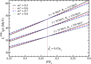
Figure 3: (Color online) Symmetry energy slope as a function of $\rho/\rho_{o}$ for the NR limit, Eq. (23). In this figure, $\rho_{o}=0.15$ fm^-3, and $B_{o}=16$ MeV.

It is worthwhile to note that the crossing density displayed in Fig. 3, namely, $\rho_{c}^{\mbox{\tiny L}}/\rho_{0}=0.47$, is exactly the same for all curves. In this figure, we group three different sets of parametrizations, each one presenting three distinct values for the pair ($J$, $K_{o}$). The values were chosen inside the ranges of $25\leqslant J\leqslant 35$ MeV, and $250\leqslant K_{o}\leqslant 315$ MeV. One can still notice that the quantity $L^{\mbox{\tiny(NR)}}(\rho_{c}^{\mbox{\tiny L}})$ is different for each set. However, the values of $L^{\mbox{\tiny(NR)}}(\rho_{c}^{\mbox{\tiny L}})$ of these parametrizations present an overlap of $48\%$ with the constraint established in Ref. slope , namely, $L(\rho_{c}^{\mbox{\tiny L}})=47.3\pm 7.8$ MeV. We still point out that the range of $25\leqslant J\leqslant 35$ MeV is showed to be totally compatible rmf with experimental values from analyses of different terrestrial nuclear experiments and astrophysical observations bali , and the range of $250\leqslant K_{o}\leqslant 315$ MeV was based on the recent reanalysis of data on isoscalar giant monopole resonance energies stone .

If we consider the expansion of $L^{\mbox{\tiny(NR)}}/(3x+1)$ until order $x$, namely, $L(\rho)\simeq(3x+1)(L_{o}+K_{\mbox{\tiny sym}}^{o}x)$, it is possible to explain the crossing point in Fig. 3 if $K_{\mbox{\tiny sym}}^{o}$ is linearly correlated with $L_{o}$, i. e., if we can write $K_{\mbox{\tiny sym}}^{o}=b_{1}+a_{1}L_{o}$, and if there exist a real root for the equation $f(x_{c})=a_{1}x_{c}+1=0$, since in this case one writes $L(\rho)=(3x+1)\left\{L_{o}\left(a_{1}x+1\right)+b_{1}x\right\}$. As we can see in Eq. (28) and in Fig. 1a, the linear correlation between $K_{\mbox{\tiny sym}}^{o}$ and $L_{o}$ holds in fact for $J$ and $K_{o}$ fixed. However, if we solve the equation $f(x_{c})=0$ we find $\rho_{c}^{\mbox{\tiny L}}/\rho_{0}=0.41$ (since $a_{1}=p(\rho_{o})=5.13$ and $\rho_{c}^{\mbox{\tiny L}}/\rho_{0}=3x_{c}^{\mbox{\tiny L}}+1$), not exactly the same crossing density presented in Fig. 3. This suggests that $f(x_{c})$ should be modified in order to produces a more exact root, what means that $L^{\mbox{\tiny(NR)}}/(3x+1)$ actually needs to be expanded in higher orders in $x$, at least in the density region around the crossing density $\rho_{c}^{\mbox{\tiny L}}/\rho_{0}=0.47$. If we now take the expansion of $L^{\mbox{\tiny(NR)}}/(3x+1)$ until order $x^{2}$, the crossing point will exist if $K_{\mbox{\tiny sym}}^{o}$ and $Q_{\mbox{\tiny sym}}^{o}$ are linearly correlated with $L_{o}$. The latter correlation is verified in Eq. (31) and Fig. 1b as we already discussed. For this case we will have

$$L(\rho)\simeq(3x+1)\left\{L_{o}+K_{\mbox{\tiny sym}}^{o}x+\frac{Q_{\mbox{\tiny sym}}^{o}}{2}x^{2}\right\}\\ =(3x+1)\left\{L_{o}\left(\frac{a_{2}}{2}x^{2}+a_{1}x+1\right)+\left(\frac{b_{2}}{2}x+b_{1}\right)x\right\},$$ (34)

with $b_{1}=q-3Jp$, $a_{1}=p$, $b_{2}=v-3Ju$, and $a_{2}=u$. The crossing is explained if $f(x_{c}^{\mbox{\tiny L}})=1+px_{c}^{\mbox{\tiny L}}+\frac{u}{2}{x_{c}^{\mbox{\tiny L}}}^{2}=0$, satisfied for

$$x_{c}^{\mbox{\tiny L}}=\frac{1}{5\left(3M^{2}-22E_{\mbox{\tiny F}}^{o}M-144E_{\mbox{\tiny F}}^{o2}\right)}\bigg{\{}15M^{2}-54E_{\mbox{\tiny F}}^{o}M-\\ (315M^{4}-2700E_{\mbox{\tiny F}}^{o}M^{3}+1676E_{\mbox{\tiny F}}^{o2}M^{2}+20160E_{\mbox{\tiny F}}^{o3}M)^{\frac{1}{2}}\bigg{\}},$$ (35)

that produces $\rho_{c}^{\mbox{\tiny L}}/\rho_{0}=0.46$, a value much more close to the crossing density than $\rho_{c}^{\mbox{\tiny L}}/\rho_{0}=0.41$, found previously.

Therefore, it becomes clear that a crossing point in a density dependence of a bulk parameters indicates a route for the searching of linear correlations in its higher order derivatives. Nevertheless, we point out to the reader that a crossing point itself does not ensure linear correlations in all higher order bulk parameters. For the previous analysis, for example, one can not affirm that $L_{o}$ will be correlated with $I_{\mbox{\tiny sym}}^{o}=(3\rho_{o})^{4}\left(\frac{\partial^{4}{\cal S}}{\partial\rho^{4}}\right)_{\rho=\rho_{o}}$, simply by the fact that the expansion of $L^{\mbox{\tiny(NR)}}/(3x+1)$ until order $x^{3}$ is better than those until order $x^{2}$. It is needed to check whether such linear correlation really holds. Actually, the crossing ensure at least the linear correlation between $L_{o}$ and the immediately next order bulk parameter $K_{\mbox{\tiny sym}}^{o}$. As a matter of fact, we investigate if $L_{o}$ correlates with $I_{\mbox{\tiny sym}}^{o}$ by obtaining the expression of the fourth order derivative of $\mathcal{S}^{\mbox{\tiny(NR)}}$, namely,

$$I_{\mbox{\tiny sym}}^{\mbox{\tiny(NR)}}(\rho)=\frac{28\lambda\rho^{\frac{2}{3}}}{3M^{2}}\left(-M+\frac{5}{7}G^{2}_{\mbox{\tiny S}}\rho-\frac{20}{7}A\rho^{2}+\frac{330}{7}B\rho^{3}\right).$$ (36)

From Eq. (36), is possible to write $I_{\mbox{\tiny sym}}^{o}=I_{\mbox{\tiny sym}}^{\mbox{\tiny(NR)}}(\rho_{o})$ in terms of $L_{o}$, $J$, $\rho_{o}$, $B_{o}$ and $K_{o}$ in the following way,

$$I_{\mbox{\tiny sym}}^{o}=(L_{o}-3J)r(\rho_{o})+s(\rho_{o},B_{o},K_{o})$$ (37)

with

$$r(\rho_{o})=\frac{20\left(3M^{2}-56ME_{\mbox{\tiny F}}^{o}+324E_{\mbox{\tiny F}}^{o2}\right)}{3M^{2}-14ME_{\mbox{\tiny F}}^{o}},$$ (38)

and

$$s(\rho_{o},B_{o},K_{o})=\frac{5}{3M^{2}-14ME_{\mbox{\tiny F}}^{o}}\times\\ \Bigg{\{}1080B_{o}E_{\mbox{\tiny F}}^{o}\left(M-2E_{\mbox{\tiny F}}^{o}\right)\\ -12E_{\mbox{\tiny F}}^{o}M\left(M-18E_{\mbox{\tiny F}}^{o}\right)-\frac{160}{3}K_{o}E_{\mbox{\tiny F}}^{o}M\Bigg{\}}.$$ (39)

Thus, it is verified that $I_{\mbox{\tiny sym}}^{o}$ also linearly correlates with $L_{o}$, under the same conditions that makes $L_{o}$ also correlated with $K_{\mbox{\tiny sym}}^{o}$ and $Q_{\mbox{\tiny sym}}^{o}$, namely, fixed values for $J$ and $K_{o}$. Furthermore, a new expansion of $L^{\mbox{\tiny(NR)}}/(3x+1)$ until order $x^{3}$ generates the cubic equation $f(x_{c}^{\mbox{\tiny L}})=1+px_{c}^{\mbox{\tiny L}}+\frac{u}{2!}{x_{c}^{\mbox{\tiny L}}}^{2}+\frac{r}{3!}{x_{c}^{\mbox{\tiny L}}}^{3}=0$, presenting a root corresponding to $\rho_{c}^{\mbox{\tiny L}}/\rho_{0}=0.47$ (since $r(0.15)=14.17$), the exact value for the crossing density.

Following these same ideas, we search for signatures of linear correlations in the Skyrme model. At this point, we remind the reader there is no unique crossing point at the density dependence of the symmetry energy and its slope for the Skyrme model, as we can see in Figs. 4 and 5, respectively, where we display the $240$ parametrizations of Ref. skyrme .

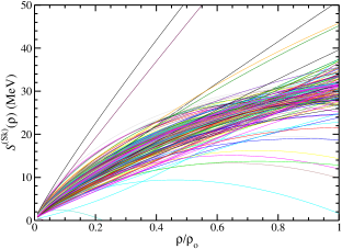
Figure 4: (Color online) Symmetry energy as a function of $\rho/\rho_{o}$ for the $240$ Skyrme parametrizations of Ref. skyrme .

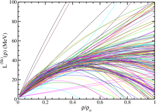
Figure 5: (Color online) Symmetry energy slope as a function of $\rho/\rho_{o}$ for the $240$ Skyrme parametrizations of Ref. skyrme .

This lack of a unique crossing in the density dependence of $\mathcal{S}(\rho)$ and $L(\rho)$ functions can also be seen in Fig. 2 (left) of Ref. corecrust , where the authors studied $21$ Skyrme parametrizations.

Specifically for the density dependence of the symmetry energy slope, we found a crossing density for the SV sv , SkO sko , SkO’ sko , SkT3 skt3 , SkRA skra and Ska35s15 skyrme parametrizations at $\rho_{c}^{\mbox{\tiny L}}/\rho_{0}=0.38$. It is displayed in Fig. 6.

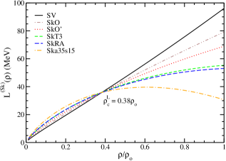
Figure 6: (Color online) Symmetry energy slope as a function of $\rho/\rho_{o}$ for some Skyrme parametrizations.

According to the discussed so far, these Skyrme parametrizations will present linear correlation at least regarding $K_{\mbox{\tiny sym}}^{o}$ and $L_{o}$. This is confirmed in Fig. 7a. Moreover, in Figs. 7b and  7c it is also checked the linear correlations of $L_{o}$ with $Q_{\mbox{\tiny sym}}^{o}$ and $I_{\mbox{\tiny sym}}^{o}$, respectively, like in the case of the NR limit.

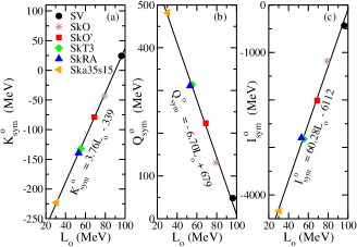
Figure 7: (Color online) (a) $K_{\mbox{\tiny sym}}^{o}$ (b) $Q_{\mbox{\tiny sym}}^{o}$, and (c) $I_{\mbox{\tiny sym}}^{o}$ as a function of $L_{o}$ for the Skyrme parametrizations of Fig. 6. The linear fits are indicated in each panel.

For the sake of completeness, we have checked that the expansion of $L(\rho)/(3x+1)$ that approaches to the exact function around $\rho/\rho_{o}=0.38$ is taken until order $x^{3}$ for these Skyrme parametrizations. Therefore, the angular coefficients found in Fig. 7 are used to define the function $f(x_{c}^{\mbox{\tiny L}})$ that needs to be null. This will provide the cubic equation $1+3.76x_{c}^{\mbox{\tiny L}}-\frac{6.70}{2!}{x_{c}^{\mbox{\tiny L}}}^{2}+\frac{60.28}{3!}{x_{c}^{\mbox{\tiny L}}}^{3}=0$, that has one of the roots given by $\rho_{c}^{\mbox{\tiny L}}/\rho_{0}=0.38$, precisely the crossing density verified in Fig. 6.

Still at the framework of the Skyrme parametrizations, another crossing point is observed in the isovector sector, specifically in the density dependence of the symmetry energy itself. As pointed out in Fig. 8, such a crossing occurs at $\rho_{c}^{\mbox{\tiny S}}/\rho_{0}=0.89$.

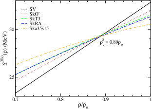
Figure 8: (Color online) Symmetry energy as a function of $\rho/\rho_{o}$ for some Skyrme parametrizations.

We have noticed that for these parametrizations, $J$ is linearly correlated with $L_{o}$, $K_{\mbox{\tiny sym}}^{o}$, $Q_{\mbox{\tiny sym}}^{o}$ and $I_{\mbox{\tiny sym}}^{o}$ as one can see in Figs. 9 and 10. The angular coefficients of these lines are used to define the quartic equation to be solved in order to determine the value of the crossing density, namely, $1+28.8x_{c}^{\mbox{\tiny S}}+\frac{108.6}{2!}{x_{c}^{\mbox{\tiny S}}}^{2}-\frac{188.3}{3!}{x_{c}^{\mbox{\tiny S}}}^{3}+\frac{1695}{4!}{x_{c}^{\mbox{\tiny S}}}^{4}=0$. One root of this equation provides the value $\rho_{c}^{\mbox{\tiny S}}/\rho_{0}=0.89$, observed in Fig. 8.

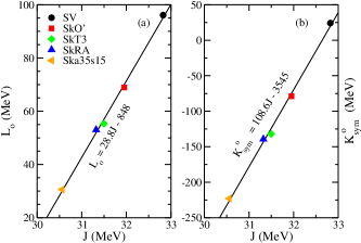
Figure 9: (Color online) (a) $L_{o}$ and (b) $K_{\mbox{\tiny sym}}^{o}$ as a function of $J$ for the Skyrme parametrizations of Fig. 8. The linear fits are indicated in each panel.

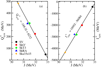
Figure 10: (Color online) (a) $Q_{\mbox{\tiny sym}}^{o}$ and (b) $I_{\mbox{\tiny sym}}^{o}$ as a function of $J$ for the Skyrme parametrizations of Fig. 8. The linear fits are indicated in each panel.

As a remark, it is worthwhile to note that a linear correlation itself between two bulk parameters is not a sufficient condition to guarantee a crossing point in the density dependence of the immediately preceding bulk parameter. As an example of this statement, we focus on the analytical structure of the NR limit to find other two specific linear correlations. From Eqs. (28) and (31) it is straightforward to obtain

$$Q_{\mbox{\tiny sym}}^{o}=\frac{u}{p}K_{\mbox{\tiny sym}}^{o}+v-\frac{uq}{p}.$$ (40)

From Eqs. (28) and (37), an analogous expression can be written relating $I_{\mbox{\tiny sym}}^{o}$ and $K_{\mbox{\tiny sym}}^{o}$, namely,

$$I_{\mbox{\tiny sym}}^{o}=\frac{r}{p}K_{\mbox{\tiny sym}}^{o}+s-\frac{rq}{p}.$$ (41)

Therefore, one see for a fixed value of $K_{o}$, that the bulk parameter $K_{\mbox{\tiny sym}}^{o}$ is linearly correlated with $Q_{\mbox{\tiny sym}}^{o}$ and $I_{\mbox{\tiny sym}}^{o}$, see Fig. 11.

Figure 11: (a) $Q_{\mbox{\tiny sym}}^{o}$ and (b) $I_{\mbox{\tiny sym}}^{o}$ as a function of $K_{\mbox{\tiny sym}}^{o}$ for the NR limit. The effective mass varies in the range of $0.50\leqslant m^{*}\leqslant 0.80$. For each panel, $\rho_{o}=0.15$ fm^-3 and $B_{o}=16$ MeV.

Here, we highlight that one can vary $K_{\mbox{\tiny sym}}^{o}$ without any information regarding $L_{o}$. Let us remind that $K_{\mbox{\tiny sym}}^{o}$ can also be written only as a function of the isoscalar parameters, according to Eq. (12) of Ref. bianca . Thus, for fixed values of $K_{o}$, it is possible to investigate how $Q_{\mbox{\tiny sym}}^{o}$ and $I_{\mbox{\tiny sym}}^{o}$ depend on $K_{\mbox{\tiny sym}}^{o}$ only from the variation of $m^{*}$.

Notice that, the expansion of $K_{\mbox{\tiny sym}}^{\mbox{\tiny(NR)}}/(3x+1)^{2}$ until order $x^{2}$ can describe the exact function in Eq. (24) in a density region of subsaturation densities, see Fig. 12a. In spite of this, the quadratic equation constructed from the angular coefficients extracted from Fig. 11, namely, $1-0.88x_{c}^{{\mbox{\tiny K}}_{\mbox{\tiny sym}}}+\frac{2.76}{2!}{x_{c}^{{\mbox{\tiny K}}_{\mbox{\tiny sym}}}}^{2}=0$, presents no real roots, indicating no crossing points in the $K_{\mbox{\tiny sym}}^{\mbox{\tiny(NR)}}(\rho)$ function. This finding is confirmed in Fig. 12b.

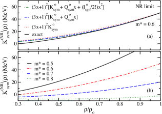
Figure 12: (Color online) $K_{\mbox{\tiny sym}}^{\mbox{\tiny(NR)}}$ as a function of $\rho/\rho_{o}$. (a) Exact function for $m^{*}=0.6$, Eq. (24), compared with its expansion. (b) Exact function for different effective mass values. The bulk parameters fixed in the two panels are $K_{o}=270$ MeV, $\rho_{o}=0.15$ fm^-3 and $B_{o}=16$ MeV.

Another example of linear correlations between bulk parameters and the lack of crossing points in the density dependence in one of them, is the case of the quantities $L_{o}$ and $J$. According to Eq. (26), a linear correlation between $J$ and $L_{o}$ is established if the function $b(m^{*},\rho_{o},B_{o},K_{o})$ is kept fixed, i. e., if the analyzed parametrizations have exactly the same isoscalar bulk parameters. Thus, parametrizations with different $J$ values but same isoscalar parameters, present the behavior depicted in Fig. 13a.

Figure 13: (a) $L_{o}\times J$ correlation obtained from Eq. (26). (b) density dependence of symmetry energy, Eq. (22).

As one can see in Fig. 13b, these parametrizations do not generate any crossing point in the density dependence of $\mathcal{S}(\rho)$. From the point of view of the discussion of Sec. II, one can understand the lack of crossing points from the equation $1+3x_{c}^{\mbox{\tiny S}}=0$, satisfied only for $x_{c}^{\mbox{\tiny S}}=-\frac{1}{3}$, i. e., for $\rho_{c}^{\mbox{\tiny S}}/\rho_{0}=0$ (since we have $\rho/\rho_{0}=3x+1$).

In summary, one can associate linear correlations as signatures of crossing points only if the exact function studied can be approximated by its expansion, and simultaneously, if the equation $f(x_{c})=0$ present nonzero real roots in the analysed range of densities. In the case of the NR limit, the latter condition is not satisfied in the study of the $K_{\mbox{\tiny sym}}^{\mbox{\tiny(NR)}}(\rho)$ function, implying in no crossing points in its density dependence in the range of subsaturation densities.

III.3 Results from the isoscalar sector

Regarding the quantities related to the isoscalar sector of the nonrelativistic hadronic models, we underline here the relationship between $K_{o}$, $Q_{o}$ and $I_{o}$. For the former two quantities, a correlation was firstly found in Refs. prl ; margueron for some Skyrme parametrizations. In particular, they found it as a linear one. Here we proceed to find, in the NR limit framework, the conditions that the parametrizations must satisfy in order to gives rise to the same relationship. For this purpose, we first need to obtain $Q(\rho,y)$ from the energy density, Eq. (18). This is done by calculating $Q=(3\rho)^{3}\left[\frac{\partial^{3}(\mathcal{E}/\rho)}{\partial\rho^{3}}\right]$, with the full expression given by

$$Q^{\mbox{\tiny(NR)}}(\rho,y)=-162B\rho^{3}+\frac{12\lambda H_{5/3}}{5M^{2}}\rho^{\frac{2}{3}}\times\\ \times\left(M-\frac{5}{4}G^{2}_{\mbox{\tiny S}}\rho+20A\rho^{2}+165B\rho^{3}\right),$$ (42)

where $Q_{o}$ is defined by $Q_{o}=Q^{\mbox{\tiny(NR)}}(\rho_{o},1/2)$.

By using the coupling constants in terms of the bulk parameters in the expressions of $K_{o}$ and $Q_{o}$, it is possible to find the following relationship between these quantities,

$$Q_{o}=i(\rho_{o})K_{o}+j(\rho_{o},B_{o},m^{*}),$$ (43)

where

$$i(\rho_{o})=\frac{3\left(9M^{2}-73E_{\mbox{\tiny F}}^{o}M+90E_{\mbox{\tiny F}}^{o2}\right)}{3M^{2}-19E_{\mbox{\tiny F}}^{o}M+18E_{\mbox{\tiny F}}^{o2}},$$ (44)

and

$$j(\rho_{o},B_{o},m^{*})=\frac{1}{3M^{2}-19E_{\mbox{\tiny F}}^{o}M+18E_{\mbox{\tiny F}}^{o2}}\times\\ \times\Bigg{\{}\frac{24E_{\mbox{\tiny F}}^{o}}{m^{*}}\left(M^{2}-40ME_{\mbox{\tiny F}}^{o}/3+60E_{\mbox{\tiny F}}^{o2}\right)\\ -162B_{o}\left(3M^{2}-25ME_{\mbox{\tiny F}}^{o}+40E_{\mbox{\tiny F}}^{o2}\right)\\ -108E_{\mbox{\tiny F}}^{o}\left(M^{2}-10ME_{\mbox{\tiny F}}^{o}+27E_{\mbox{\tiny F}}^{o2}\right)\Bigg{\}}.$$ (45)

From the structure presented in Eq. (43), we notice that the effective mass plays a crucial role for the correlation between $Q_{o}$ and $K_{o}$. For fixed values of $m^{*}$, this correlation is a linear one. We remember the reader that $\rho_{o}$ and $B_{o}$ vary only in a very narrow range around $0.15$ fm^-3 and $16$ MeV, respectively. Thus, these bulk parameters can be considered constants for the hadronic mean-field models. For different $m^{*}$ values, Eq. (43) generates parallel lines as indicated in Fig. 14a. The same linear correlation is also observed in some Gogny parametrizations, as indicated in Fig. 14b.

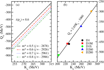
Figure 14: (Color online) $Q_{o}$ as a function of $K_{o}$ for (a) the NR limit with different $m^{*}$ values, and for (b) some Gogny parametrizations studied in Ref. gogny . In panel (a), $\rho_{o}=0.15$ fm^-3 and $B_{o}=16$ MeV.

From the perspective addressed in Sec. II, the linear correlation between $K_{o}$ and $Q_{o}$ could also be sought, by searching for a possible crossing point in the density dependence of the incompressibility. In fact, as pointed out in Fig. 15, there are two of them, at $\rho_{c}^{\mbox{\tiny K}}/\rho_{0}=0.21$ (not shown), and $\rho_{c}^{\mbox{\tiny K}}/\rho_{0}=0.79$.

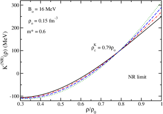
Figure 15: (Color online) Incompressibility as a function of $\rho/\rho_{o}$ for the NR limit, Eq. (21).

Furthermore, notice that the the second point is quite close to the crossing density $\rho_{c}^{\mbox{\tiny K}}/\rho_{0}=0.71$ observed also for the Skyrme parametrizations studied in Ref. margueron .

Since crossings in the $K^{\mbox{\tiny(NR)}}(\rho)$ function were found, they indicate a signature of a linear correlation, in this case at least between $K_{o}$ and $Q_{o}$, since the latter is the bulk parameter associated to the immediately next order derivative of $K(\rho)$. Nevertheless, for the NR limit, we can also check analytically if the next bulk parameter, $I_{o}$, correlates with $K_{o}$. From Eq. (18) and the definition $I=(3\rho)^{3}\left[\frac{\partial^{3}(\mathcal{E}/\rho)}{\partial\rho^{3}}\right]$, one obtains,

$$I^{\mbox{\tiny(NR)}}(\rho,y)=\frac{84\lambda H_{5/3}}{5M^{2}}\rho^{\frac{2}{3}}\times\\ \times\left(-M+\frac{5}{7}G^{2}_{\mbox{\tiny S}}\rho-\frac{20}{7}A\rho^{2}+\frac{330}{7}B\rho^{3}\right).$$ (46)

From this expression, the fourth order derivative of the energy per particle evaluated at the saturation density, $I_{o}=I^{\mbox{\tiny(NR)}}(\rho_{o},1/2)$, can be written in terms of $\rho_{o}$, $B_{o}$, $m^{*}$, and $K_{o}$ as

$$I_{o}=w(\rho_{o})K_{o}+z(\rho_{o},B_{o},m^{*}),$$ (47)

where

$$w(\rho_{o})=-\frac{20\left(25E_{\mbox{\tiny F}}^{o}M-54E_{\mbox{\tiny F}}^{o2}\right)}{3M^{2}-19E_{\mbox{\tiny F}}^{o}M+18E_{\mbox{\tiny F}}^{o2}},$$ (48)

and

$$z(\rho_{o},B_{o},m^{*})=\frac{1}{3M^{2}-19E_{\mbox{\tiny F}}^{o}M+18E_{\mbox{\tiny F}}^{o2}}\times\\ \times\Bigg{\{}\frac{40E_{\mbox{\tiny F}}^{o}}{m^{*}}\left(3M^{2}-56ME_{\mbox{\tiny F}}^{o}+324E_{\mbox{\tiny F}}^{o2}\right)\\ +1080B_{o}\left(9ME_{\mbox{\tiny F}}^{o}-32E_{\mbox{\tiny F}}^{o2}\right)\\ -72E_{\mbox{\tiny F}}^{o}\left(4M^{2}-77ME_{\mbox{\tiny F}}^{o}+324E_{\mbox{\tiny F}}^{o2}\right)\Bigg{\}}.$$ (49)

Notice that once more, the effective mass needs to be constant for the parametrizations in order to ensure a linear dependence between $I_{o}$ and $K_{o}$, with angular coefficient given by $w(0.15)=-4.16$.

For the sake of completeness, we use the angular coefficients $i(\rho_{o})$ and $w(\rho_{o})$ to calculate the crossing density in Fig. 15. First, we consider the energy per particle of symmetric nuclear matter as

$$E(\rho)\simeq E_{o}+\frac{K_{o}}{2!}x^{2}+\frac{Q_{o}}{3!}x^{3}+\frac{I_{o}}{4!}x^{4},$$ (50)

then, the corresponding expansion for $K(\rho)$ reads

$$K (\rho)=18\rho\frac{\partial E}{\partial\rho}+9\rho^{2}\frac{\partial^{2}E}{\partial\rho^{2}}$$

$$= 6(3x+1)\frac{\partial E}{\partial x}+(3x+1)^{2}\frac{\partial^{2}E}{\partial x^{2}}$$

$$\simeq (3x+1)\times$$

$$\times \left[K_{o}+(9K_{o}+Q_{o})x+\left(6Q_{o}+\frac{I_{o}}{2}\right)x^{2}+\frac{5I_{o}}{2}x^{3}\right].\quad\,\,\,\,\,$$ (52)

This expansion is observed to be consistent with the exact function, Eq. (21), as showed in Fig. 16.

Figure 16: (Color online) Density dependence of the incompressibility compared with its expansion for the NR limit.

It is worth noting that despite the extra term in Eq. (III.3) compared with $\mathcal{F}^{\prime\prime}$ in Eq. (5), the final expansion, Eq. (52), is analogous to the general function $\mathcal{F}^{(m)}(\rho)$ in Eq. (7). Therefore, all the procedure developed in Sec. II also applies in the analysis of correlations and crossing points for the $K^{\mbox{\tiny(NR)}}(\rho)$ function in the isoscalar sector. Indeed, this was done for some Skyrme parametrizations in Ref. margueron . From this point of view, it is possible to use Eqs. (43) and (47) to rewrite Eq. (52) as

$$K(\rho)=(3x+1)\times\\ \times\left\{K_{o}\left[1+(9+i)x+\left(6i+\frac{w}{2}\right)x^{2}+\frac{5w}{2}x^{3}\right]\right.\\ +\left.\left[j+\left(6j+\frac{z}{2}\right)x+\frac{5z}{2}x^{2}\right]x\right\}.$$ (53)

Thus, the crossings points in Fig. 15a are justified if $1+(9+i)x_{c}^{\mbox{\tiny K}}+(6i+w/2){x_{c}^{{\mbox{\tiny K}}}}^{2}+(5w/2){x_{c}^{{\mbox{\tiny K}}}}^{3}=0$. Two solutions of this cubic equation are $\rho_{c}^{\mbox{\tiny K}}/\rho_{0}=0.21$, and $\rho_{c}^{\mbox{\tiny K}}/\rho_{0}=0.79$.

IV Correlations in FR-RMF models

In the context of QHD, protons and neutrons are the fundamental particles interacting each other through scalar and vector mesons exchange. In this framework, the fields $\sigma$ and $\omega$ represent, respectively, these mesons and mimic the attractive and repulsive parts of the nuclear interaction. The main representative of QHD models is the Walecka one walecka , in which the only two free parameters are fitted in order to reproduce the values of $\rho_{o}$ and $B_{o}$. However, it does not give reasonable values for $K_{o}$ ($\sim 500$ MeV), and $M^{*}_{o}$ ($\sim 0.54M$). This problem was circumvented by Boguta and Bodmer boguta , who added to the Walecka model cubic and quartic self-interactions in the scalar field $\sigma$, introducing, consequently, two more free parameters, which are fitted so as to fix these quantities. All thermodynamic quantities of this model are found from its Lagrangian density, given by

$$\mathcal{L} = \overline{\psi}(i\gamma^{\mu}\partial_{\mu}-M)\psi+g_{\sigma}\sigma\overline{\psi}\psi+\frac{1}{2}(\partial^{\mu}\sigma\partial_{\mu}\sigma-m^{2}_{\sigma}\sigma^{2})$$ (54)

$$- \frac{A}{3}\sigma^{3}-\frac{B}{4}\sigma^{4}-g_{\omega}\overline{\psi}\gamma^{\mu}\omega_{\mu}\psi-\frac{1}{4}F^{\mu\nu}F_{\mu\nu}+\frac{1}{2}m^{2}_{\omega}\omega_{\mu}\omega^{\mu}$$

$$- \frac{g_{\rho}}{2}\overline{\psi}\gamma^{\mu}\vec{\rho}_{\mu}\vec{\tau}\psi-\frac{1}{4}\vec{B}^{\mu\nu}\vec{B}_{\mu\nu}+\frac{1}{2}m^{2}_{\rho}\vec{\rho}_{\mu}\vec{\rho}^{\mu},$$

with $F_{\mu\nu}=\partial_{\nu}\omega_{\mu}-\partial_{\mu}\omega_{\nu}$, and $\vec{B}_{\mu\nu}=\partial_{\nu}\vec{\rho}_{\mu}-\partial_{\mu}\vec{\rho}_{\nu}-g_{\rho}(\vec{\rho}_{\mu}\times\vec{\rho}_{\nu})$. The coupling constants are $g_{\sigma}$, $g_{\omega}$, $g_{\rho}$, $A$ and $B$. For a complete description of the model, and also other kind of FR-RMF ones, such as density dependent, crossed terms and nonlinear point-couplings, we address the reader to the recent study of Ref. rmf involving an analysis of $263$ relativistic parametrizations under constraints related to symmetric nuclear matter, pure neutron matter, symmetry energy, and its derivatives. Here, we mainly focus in searching for correlations between bulk parameters for the FR-RMF parametrizations described by Eq. (54).

IV.1 Isovector sector

Besides its complete analytical structure, other advantage of the NR limit of NLPC models is its usefulness in predictions of correlations in Boguta-Bodmer models, as pointed out in Ref. bianca . For instance, the $L_{o}\times J$ correlation in Eq. (26) is showed to be linear also for these models under the restriction of fixed values of effective mass. Like in the NR limit, different values for $K_{o}$ do not destruct the linear dependence, see figure 2b of Ref. bianca . Based on this correspondence, we use the framework of the NR limit to confirm other correlations in Boguta-Bodmer models. Still at the isovector sector, we showed in Ref. bianca that the linear correlation indicated in Eq. (28) holds for the models described by Eq. (54), if we also fix the values of $K_{o}$ and $J$. Now, we further investigate such a correlation. In Fig. 17, we show $K_{\mbox{\tiny sym}}^{o}$ as a function of $L_{o}$ for parametrizations with effective masses submitted to the FRS constraint, Eq. (1). According to Ref. ls-splitting , this is the range of $m^{*}$ in which Boguta-Bodmer models have to be constrained in order to produce spin-orbit splittings in agreement with well established experimental values for the ${}^{16}\rm{O}$, ${}^{40}\rm{Ca}$, and ${}^{208}\rm{Pb}$ nuclei.

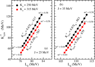
Figure 17: (Color online) $K_{\mbox{\tiny sym}}^{o}$ versus $L_{o}$ for Boguta-Bodmer models with $\rho_{o}=0.15$ fm^-3 and $B_{o}=16$ MeV. The linear fittings are indicated in both panels.

In this figure, we present curves corresponding to the limiting values of the ranges $25\leqslant J\leqslant 35$ MeV rmf , and $250\leqslant K_{o}\leqslant 315$ MeV stone .

From these results, we can conclude that the relation $K_{\mbox{\tiny sym}}^{o}=p_{rel}L_{o}+q_{rel}$ also works well for the Boguta-Bodmer models submitted to the FRS constraint. However, by comparing the angular coefficients $p(\rho_{o})$ from Eq. (28) and $p_{rel}$, we notice that $p_{rel}$ slightly depends on $K_{o}$, unlike the nonrelativistic case in which the angular coefficient depends only on $\rho_{o}$. We perform the same analysis for the $L_{o}$ dependence on $Q_{\mbox{\tiny sym}}^{o}$, motivated by the linear correlation presented in Eq. (31). The result is found in Fig. 18.

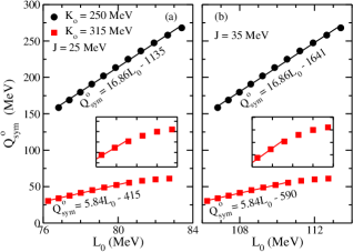
Figure 18: (Color online) $Q_{\mbox{\tiny sym}}^{o}$ versus $L_{o}$ for Boguta-Bodmer models with $\rho_{o}=0.15$ fm^-3, $B_{o}=16$ MeV, and $0.58\leqslant m^{*}\leqslant 0.64$. The linear fittings are indicated in both panels. In the insets, we show $L_{o}$ in the ranges of (a) $79\leqslant L_{o}\leqslant 83$ MeV, and (b) $109\leqslant L_{o}\leqslant 113$ MeV.

As we see, there is a correlation between $Q_{\mbox{\tiny sym}}^{o}$ and $L_{o}$. However, the linear form $Q_{\mbox{\tiny sym}}^{o}=u_{rel}L_{o}+v_{rel}$ is strongly dependent on $K_{o}$, unlike the previous case. For $K_{o}=315$ MeV, for example, we notice the range of effective mass that still ensure a line in the curve fitting is reduced from the range of Eq. (1) to $0.60\leqslant m^{*}\leqslant 0.64$. The break of this linearity is better depicted in the insets of Fig. 18.

One can also use the linear dependences showed in Figs. 17 and 18, with the latter guaranteed only for some values of $K_{o}$ and $m^{*}$, in order to justify a possible crossing point in the density dependence of the symmetry energy slope, as we did in the case of nonrelativistic models in Sec. III. In fact, there is such a crossing as we can see in Fig. 19.

Figure 19: (Color online) Symmetry energy slope as a function of $\rho/\rho_{o}$ for some Boguta-Bodmer parametrizations.

From the angular coefficients of the respective lines of Figs. 17a and 18a, we can solve the equation $1+8.87x_{c}^{\mbox{\tiny L}}+\frac{16.86}{2!}{x_{c}^{\mbox{\tiny L}}}^{2}=0$ to find a crossing density at $\rho_{c}^{\mbox{\tiny L}}/\rho_{0}=0.61$. This value can not be refined since a linear correlation is not found in the next order bulk parameter, namely, $I_{\mbox{\tiny sym}}^{o}$, as we see in Fig. 20.

Figure 20: (Color online) $I_{\mbox{\tiny sym}}^{o}$ versus $L_{o}$ for Boguta-Bodmer models with $\rho_{o}=0.15$ fm^-3, $B_{o}=16$ MeV, and $0.58\leqslant m^{*}\leqslant 0.64$.

We see that a correlation between $L_{o}$ and $I_{\mbox{\tiny sym}}^{o}$ holds for the relativistic Boguta-Bodmer models, but it is not a linear one, as we verified in the NR limit, Eq. (37).

Still concerning isovector bulk parameters, we point out to the reader a specif class of relativistic models of Ref. cai with mesonic crossed interactions. Following notation of Ref. rmf , they are classified as type 4 models ($\sigma^{3}+\sigma^{4}+\omega_{0}^{4}+$ cross terms models) and have the terms,

$$\mathcal{L}_{\sigma\omega\rho}=g_{\sigma}g_{\omega}^{2}\sigma\omega_{\mu}\omega^{\mu}\left(\alpha_{1}+\frac{1}{2}{\alpha_{1}}^{\prime}g_{\sigma}\sigma\right)+\frac{C}{4}(g_{\omega}^{2}\omega_{\mu}\omega^{\mu})^{2}\\ +\frac{1}{2}{\alpha_{3}}^{\prime}g_{\omega}^{2}g_{\rho}^{2}\omega_{\mu}\omega^{\mu}\vec{\rho}_{\mu}\vec{\rho}^{\mu}+g_{\sigma}g_{\rho}^{2}\sigma\vec{\rho}_{\mu}\vec{\rho}^{\mu}\left(\alpha_{2}+\frac{1}{2}{\alpha_{2}}^{\prime}g_{\sigma}\sigma\right)$$ (55)

added to the Lagrangian density of Eq. (54). The parametrizations of this model presented in Ref. cai are constructed in order to fix the symmetry energy not at the saturation density, but in a smaller value. They present $\mathcal{S}(\rho_{c}^{\mbox{\tiny S}})=26$ MeV, with $\rho_{c}^{\mbox{\tiny S}}/\rho_{o}=0.68$. Therefore, the $\mathcal{S}(\rho)$ function presents a crossing point, as pointed out in Ref. 19 , and as one can see in Fig. 21a.

Figure 21: (Color online) (a) Symmetry energy as a function of $\rho/\rho_{o}$, and (b) $L_{o}$ as a function of $J$ for the parametrizations of Ref. cai .

Therefore, such a crossing indicates a linear behavior between $L_{o}$ and $J$ for these specific parametrizations. This correlation is clearly observed in Fig. 21b. Furthermore, the crossing density is obtained from the angular coefficient, by solving the equation $1+9.27x_{c}^{\mbox{\tiny S}}=0$. The solution of this linear equation leads to $\rho_{c}^{\mbox{\tiny S}}/\rho_{0}=0.68$, exactly the value verified in Fig. 21a.

As a last remark of this subsection, we point out to the reader that the angular and linear coefficients of the $L_{o}\times J$ correlation are not universal, as we can see by comparing the linear equation of Fig. 21b of the relativistic FSU family, with that of Fig. 9a of the Skyrme parametrizations. Even among relativistic models, one can not reach such universality, as we can see by the comparison of the correlation in Fig. 21b with that found in Ref. ellipses for the relativistic NL3* and IU-FSU families.

IV.2 Isoscalar sector

Motivated by the analytical structure relating $K_{o}$, $Q_{o}$, and $I_{o}$, we investigate in this section whether the linear dependences presented in the NR limit, see Eqs. (43) and (47), also applies for Boguta-Bodmer models. According to the NR limit case, if we keep fixed the effective mass, $K_{o}$ linearly correlates with $Q_{o}$ as we show in Eq. (43) and Fig. 14a. For the relativistic case of FR-RMF models described by Eq. (54), we see that this condition remains, as one can see in Fig. 22a for the MS2 ms2 , NLSH nlsh , NL4 nl4 , NLRA1 nlra1 , Q1 q1 , Hybrid hybrid , NL3 nlsh , FAMA1 fama1 , NL-VT1 nlvt1 , NL06 rmf , and NLS nls parametrizations presenting $m^{*}\simeq 0.6$.

Figure 22: (Color online) (a) $Q_{o}$ as a function of $K_{o}$ for some Boguta-Bodmer parametrizations with $m^{*}\simeq 0.6$. (b) Incompressibility as a function of $\rho/\rho_{o}$ for the same parametrizations.

Such a correlation can be used in order to justify the crossing in the $K(\rho)$ function depicted in Fig. 22b. Proceeding in that direction, we use the expansion of the energy per particle in Eq. (50) until order $x^{3}$ to calculate the density dependence of the incompressibility. The result of this calculation is given by

$$K(\rho)\simeq(3x+1)\left[K_{o}+(9K_{o}+Q_{o})x+6Q_{o}x^{2}\right].$$ (56)

Therefore, the linear dependence $Q_{o}=i_{rel}K_{o}+j_{rel}$ showed in Fig. 22a can be used in Eq. (56) to furnish

$$K(\rho) \simeq (3x+1)\left\{K_{o}\left[1+(9+i_{rel})x+6ix^{2}\right]\right.$$ (57)

$$+ \left.\left(1+6x\right)j_{rel}x\right\},$$

with $i_{rel}=6.30$ and $j_{rel}=1552$ MeV. Thus, one has a crossing point when the quadratic equation $1+(9+i_{rel})x_{c}^{\mbox{\tiny K}}+6i_{rel}{x_{c}^{{\mbox{\tiny K}}}}^{2}=0$ present solution. This is the case for $\rho_{c}^{\mbox{\tiny K}}/\rho_{0}=0.78$.

We remark that a crossing point in the $K(\rho)$ function was firstly explained from the linear correlation between $K_{o}$ and $Q_{o}$ in Ref. margueron . However, the authors found such a crossing for some nonrelativistic Skyrme and Gogny parametrizations. For the relativistic models analysed, they did not found linear correlations or crossing points. Indeed, for the nonrelativistic case, they found a crossing at $\rho_{c}^{\mbox{\tiny K}}/\rho_{0}\simeq 0.7$, a value quite close to ours findings, namely, $\rho_{c}^{\mbox{\tiny K}}/\rho_{0}=0.77$ and $\rho_{c}^{\mbox{\tiny K}}/\rho_{0}=0.79$, for Boguta-Bodmer models and the NR limit, respectively, see Figs. 22b and 15.

Unlike the linear correlation presented in the NR limit, the angular coefficient $i_{rel}$ is slightly dependent on the effective mass. For the former case, we have $i=i(\rho_{o})$, see Eq. (44). In Fig. 23, we show this variation observing the FRS constraint and the range $250\leqslant K_{o}\leqslant 315$ MeV.

Figure 23: (Color online) $Q_{o}$ as a function of $K_{o}$ for Boguta-Bodmer parametrizations in which $\rho_{o}=0.15$ fm^-3 and $B_{o}=16$ MeV. The linear fittings are indicated in the figure.

In particular, notice that for $m^{*}=0.64$, a value that ensure good values for finite nuclei spin-orbit splittings ls-splitting , the range of the skewness coefficient is given by $-183\leqslant Q_{o}\leqslant 130$ MeV. Such a specific constraint for $Q_{o}$ present an overlap of $\simeq 36\%$ with a recent range proposed for this bulk parameter in Ref. chen-skew , namely, $-494\leqslant Q_{o}\leqslant-10$ MeV. In this study, the authors analysed models with crossed interactions among the fields, i. e., models described by Eq. (54) added to the terms in Eq. (55). They verified that such models, presenting the skewness coefficient in the range of $-494\leqslant Q_{o}\leqslant-10$ MeV, satisfy the suprasaturation constraint for the density dependence of the pressure in the symmetric nuclear science , and also the neutron star mass constraint, given by $2.01\pm 0.04M_{\odot}$. This latter is due to the recently discovered neutron star PSR J0348+0432 ns .

Finally, we verify whether the relationship between $K_{o}$ and $I_{o}$ presented in Eq. (47) is preserved in the relativistic case. According to the results of Fig. 24a, we see that the linear behavior $I_{o}=w_{rel}K_{o}+z_{rel}$ still remains in the range of $250\leqslant K_{o}\leqslant 315$ MeV, with $w_{rel}$ slightly depending on $m^{*}$, like in the case of $i_{rel}$.

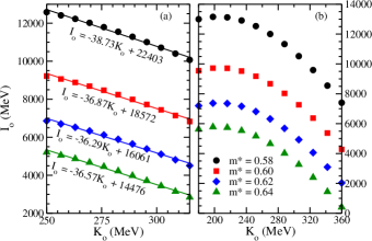
Figure 24: (Color online) $I_{o}$ as a function of $K_{o}$ for Boguta-Bodmer parametrizations in which $\rho_{o}=0.15$ fm^-3 and $B_{o}=16$ MeV. The curves are constructed in the range of (a) $250\leqslant K_{o}\leqslant 315$ MeV, and (b) $180\leqslant K_{o}\leqslant 360$ MeV. The linear fittings are indicated in panel (a).

It is worth to notice that, as showed in Fig. 24b, for a broader range of $K_{o}$ the linear dependence is blurred, although a correlation between the bulk parameters $K_{o}$ and $I_{o}$ still remains.

V Models with more than one isovector coupling constant

In previous sections, we have analyzed under what conditions the linear correlations presented in the NR limit of point-coupling models are reproduced in the context of relativistic Boguta-Bodmer parametrizations. However, our comparisons were restricted to relativistic and nonrelativistic models presenting only one isovector coupling constant, namely, $g_{\rho}$ and $G^{2}_{\mbox{\tiny TV}}$, respectively. For the Boguta-Bodmer model, $g_{\rho}$ is related to the interaction strength between the nucleon and the $\rho$ meson. For the NR limit model, $G^{2}_{\mbox{\tiny TV}}$ regulates the strength of the term that mimics the same kind of interaction (we remind the reader that our NR limit model is derived from a relativistic point-coupling model, therefore, a model in which there are no meson exchanges). Regarding the specific relationship between $L_{o}$ and $J$, we concluded in Ref. bianca that for the NR limit model, such correlation is linear whenever the isoscalar bulk parameters, namely, $m^{*}$, $\rho_{o}$, $B_{o}$ and $K_{o}$, remain unchanged. We also showed that this same condition also ensures a linear correlation between $L_{o}$ and $J$ for Boguta-Bodmer parametrizations. Furthermore, the angular coefficients of these correlations are the same, and the absolute values of $L_{o}$ are very close each other, as we can see in Fig. 25 for the NL3* Boguta-Bodmer parametrizations and their respective NR limit versions, namely, the NR-NL3* ones.

Figure 25: $L_{o}$ as a function of $J$ for the NL3* Boguta-Bodmer parametrizations and their NR limit versions NR-NL3*. These parametrizations were constructed by fixing $\rho_{o}=0.15$ fm^-3, $B_{o}=16.31$ MeV, $m^{*}=0.594$, $K_{o}=258.25$ MeV, and by running $J$.

In order to construct this figure, we fixed the isoscalar parameters values of the NL3* model, and varied the $J$ values. We taken such procedure for the exact relativistic NL3* parametrization, and for its NR limit version. For the latter, we have used our Eq. (26).

By proceeding one step further in our analysis of the $L_{o}\times J$ correlation, we now study relativistic and nonrelativistic models with more than one isovector parameter in order to verify whether the dependence observed in Fig. 25 still applies. For the relativistic model, we use that described by the Lagrangian density of Eq. (54) added to those of Eq. (55) with $\alpha_{1}=\alpha_{2}=\alpha^{\prime}_{1}=\alpha^{\prime}_{2}=C=0$, i. e., we choose a model with interaction between the mesons $\omega$ and $\rho$. Thus, we are dealing with a model with two isovector parameters, namely, $g_{\rho}$ and $\alpha^{\prime}_{3}$.

To take the NR limit of this specific model, we construct the following point-coupling Lagrangian density,

$$\mathcal{L}_{\mbox{\tiny NLPC}} = \bar{\psi}(i\gamma^{\mu}\partial_{\mu}-M)\psi-\frac{1}{2}G^{2}_{\mbox{\tiny V}}(\bar{\psi}\gamma^{\mu}\psi)^{2}+\frac{1}{2}G^{2}_{\mbox{\tiny S}}(\bar{\psi}\psi)^{2}$$ (58)

$$+ \frac{A}{3}(\bar{\psi}\psi)^{3}+\frac{B}{4}(\bar{\psi}\psi)^{4}-\frac{1}{2}G^{2}_{\mbox{\tiny TV}}(\bar{\psi}\gamma^{\mu}\vec{\tau}\psi)^{2}$$

$$- \frac{1}{4}G_{\mbox{\tiny VTV}}(\bar{\psi}\gamma^{\mu}\vec{\tau}\psi)^{2}(\bar{\psi}\gamma^{\mu}\psi)^{2},$$

in which the last term mimics the interaction between the mesons $\omega$ and $\rho$. The isovector coupling constants of this model are $G^{2}_{\mbox{\tiny TV}}$ and $G_{\mbox{\tiny VTV}}$. The symmetry energy and its slope for the NR limit of this model are given by,

$$\mathcal{S}^{\mbox{\tiny(NR)}}(\rho)=G^{2}_{\mbox{\tiny TV}}\rho+G_{\mbox{\tiny VTV}}\rho^{3}+\frac{\lambda\rho^{\frac{2}{3}}}{6M^{*}(\rho,1/2)},$$ (59)

and

$$L^{\mbox{\tiny(NR)}}(\rho) = \frac{\lambda\rho^{\frac{2}{3}}}{3M^{2}}\left(M+\frac{5}{2}G^{2}_{\mbox{\tiny S}}\rho+8A\rho^{2}+\frac{33}{2}B\rho^{3}\right)$$ (60)

$$+ 3G^{2}_{\mbox{\tiny TV}}\rho+9G_{\mbox{\tiny VTV}}\rho^{3},$$

respectively. The new isovector coupling constant, $G_{\mbox{\tiny VTV}}$, is found by imposing upon the model that the symmetry energy at $\rho_{1}/\rho_{o}\equiv r$ is fixed at a particular value $\mathcal{S}_{1}\equiv\mathcal{S}(\rho_{1})$. Here, $r$ is a value smaller than $1$. Furthermore, we still found $G^{2}_{\mbox{\tiny TV}}$ by requiring that the model present a particular value $J$ for the symmetry energy at the saturation density. The analytical form of these constants as a function of the bulk parameters can be found in the Appendix.

Such an analytical structure enables us to find the following correlation between $L_{o}$ and $J$,

$$L_{o}=3\left(\frac{3-r^{2}}{1-r^{2}}\right)J+b^{\prime}(m^{*},\rho_{o},B_{o},K_{o},r,\mathcal{S}_{1}),$$ (61)

with

$$b^{\prime} (m^{*},\rho_{o},B_{o},K_{o},r,\mathcal{S}_{1})=b(m^{*},\rho_{o},B_{o},K_{o})$$

$$+ \frac{10E_{\mbox{\tiny F}}^{o}r^{2/3}}{3(r^{2}-1)(3M^{2}-19E_{\mbox{\tiny F}}^{o}M+18E_{F}^{o2})}\times$$

$$\times \Bigg{\{}\frac{E_{\mbox{\tiny F}}^{o}}{3m^{*}}\left(13M-66E_{\mbox{\tiny F}}^{o}\right)+\frac{K_{o}}{6}\left(M-6E_{\mbox{\tiny F}}^{o}\right)$$

$$- B_{o}\left(9M-48E_{\mbox{\tiny F}}^{o}\right)-E_{\mbox{\tiny F}}^{o}\left(7M-36E_{\mbox{\tiny F}}^{o}\right)$$

$$- r\bigg{[}\frac{16E_{\mbox{\tiny F}}^{o}}{3m^{*}}\left(M-6E_{\mbox{\tiny F}}^{o}\right)+\frac{2}{3}K_{o}\left(M-3E_{\mbox{\tiny F}}^{o}\right)$$

$$- 6B_{o}\left(3M-13E_{\mbox{\tiny F}}^{o}\right)-2E_{\mbox{\tiny F}}^{o}\left(5M-27E_{\mbox{\tiny F}}^{o}\right)\bigg{]}$$

$$- r^{2}\bigg{[}-\frac{E_{\mbox{\tiny F}}^{o}}{m^{*}}\left(M-10E_{\mbox{\tiny F}}^{o}\right)-\frac{K_{o}}{2}\left(M-2E_{\mbox{\tiny F}}^{o}\right)$$

$$+ 3B_{o}\left(3M-10E_{\mbox{\tiny F}}^{o}\right)+3E_{\mbox{\tiny F}}^{o}\left(M-6E_{\mbox{\tiny F}}^{o}\right)\bigg{]}\Bigg{\}}$$

$$+ \frac{6}{(r^{2}-1)}\Bigg{[}\frac{\mathcal{S}_{1}}{r}+\frac{5E_{\mbox{\tiny F}}^{o}}{9m^{*}}(1-r^{2/3})+\frac{5E_{\mbox{\tiny F}}^{o}}{9}(r^{2/3}-r^{-1/3})\Bigg{]}.$$

Notice that now, a linear correlation between $L_{o}$ and $J$ is established if the function $b^{\prime}(m^{*},\rho_{o},B_{o},K_{o},r,\mathcal{S}_{1})$ is a constant, i. e., if the quantities $m^{*}$, $\rho_{o}$, $B_{o}$, $K_{o}$, $r$, and $\mathcal{S}_{1}$ are kept fixed. Moreover, if we now look at the $\mathcal{S}(\rho)$ function for a particular parametrization family, namely, that in which the set $m^{*}$, $\rho_{o}$, $B_{o}$, $K_{o}$, $r$, and $\mathcal{S}_{1}$ is fixed and $J$ runs a certain range, we see a crossing point, differently from the NR limit case presenting only one isovector coupling constant. We show this finding in Fig. 26 for the NR-NL3* family.

Figure 26: Density dependence of the symmetry energy for the NR-NL3* parametrization family with two isovector parameters.

By looking at the finite range relativistic model with the $\omega$ and $\rho$ mesons interaction, we verified that a linear correlation between $L_{o}$ and $J$ also holds if we apply the same conditions observed in the NR limit case, i. e., fixed values of $m^{*}$, $\rho_{o}$, $B_{o}$, $K_{o}$, $r$, and $\mathcal{S}_{1}$. A direct comparison between these two correlations, analogous to that presented in Fig. 25, is displayed in Fig. 27.

Figure 27: $L_{o}$ as a function of $J$ for the relativistic NL3* parametrization family and their NR limit versions NR-NL3*. These parametrizations were constructed by fixing $\rho_{o}=0.15$ fm^-3, $B_{o}=16.31$ MeV, $m^{*}=0.594$, $K_{o}=258.25$ MeV, $r=0.67$, $\mathcal{S}_{1}=25.8$ MeV, and by running $J$. Both models present two isovector coupling constants.

Here, we restricted our analysis for $J$ in a range of values greater than $\mathcal{S}_{1}$.

From Fig. 27, we can notice that the NR limit version of NL3* parametrizations with two isovector coupling constants, presents a different slope for the $L_{o}\times J$ linear correlation, differently from the case showed in Fig. 25, where we tested models with only one isovector parameter. This result is in qualitative agreement with the findings obtained in Ref. ellipses , where the authors compared the same NL3* parametrization family (two isovector parameters) with a nonrelativistic Skyrme parametrization family named as SkNL3*. For this family, the isoscalar bulk parameters present the same values as in the relativistic NL3* model. The authors also imposed that the energy per neutron predictions, at subsaturation densities, of the SkNL3* and NL3* models were compatible with the band constraint depicted in Fig. 2 of Ref. ellipses . As a consequence, they found correlation bands (ellipses) for the $L_{o}$ and $J$ bulk parameters, as one can see in Fig. 28.

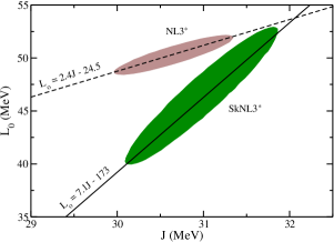
Figure 28: (Color online) Correlation bands for the $L_{o}$ and $J$ bulk parameters of the NL3* parametrization family and SkNL3* one, extracted from Fig. 3a of Ref. ellipses . The full lines are linear fits.

These ellipses were constructed by the authors of Ref. ellipses from the covariance analysis method. In Fig. 28, we extracted such bands and constructed the linear fits. Notice the nonrelativistic line presenting a greater slope in comparison with the relativistic one, exactly the same qualitative behavior observed in Fig. 27, where we have constructed the correlations only observing the conditions under which they are linear ones. Furthermore, our ratio for the NL3* slope to the NR-NL3* one is not much different to the same ratio of Fig. 28, namely, $2.22$ for ours (Fig. 27), and $2.96$ for Ref. ellipses , or Fig. 28, obtained from the covariance analysis method.

VI Summary and conclusions

In this work, we analysed the arising of correlations between isovector and isoscalar bulk parameters of hadronic nonrelativistic, and relativistic mean-field models. In particular, we discussed the connection of the crossing point in the density dependence of a particular bulk quantity, with the specific linear correlation between this quantity with its immediately next order bulk parameter. In the isovector sector, for instance, if there is a crossing point in the density dependence of the symmetry energy, then, it can be explained by the linear correlation between the symmetry energy, $\mathcal{S}$, and its slope, $L=3\rho(\partial\mathcal{S}/\partial\rho)$, both evaluated at the saturation density, i. e., there will be a linear correlation between $J=\mathcal{S}(\rho_{o})$ and $L_{o}=L(\rho_{o})$. In summary, the crossing points can be seen as a signature, or a route, in the searching of linear correlations among bulk parameters, as discussed in Sec. II.

In the nonrelativistic framework, we presented correlations in some Skyrme skyrme and Gogny parametrizations, see Figs. 2, 7, 9, 10 and 14b, as well as in parametrizations generated from the NR limit of NLPC models. By using the analytical structure of the latter model, we could write its five coupling constants in terms of the bulk parameters $\rho_{o}$, $B_{o}$, $K_{o}$, $m^{*}$, and $J$ in order to investigate the conditions in which the linear correlations of $L_{o}$ with $K_{\mbox{\tiny sym}}^{o}$, $Q_{\mbox{\tiny sym}}^{o}$ and $I_{\mbox{\tiny sym}}^{o}$, in the isovector sector, and of $K_{o}$ with $Q_{o}$ and $I_{o}$, in the isoscalar one holds. For these parametrizations, we showed that $L_{o}$ linearly correlates with $K_{\mbox{\tiny sym}}^{o}$, $Q_{\mbox{\tiny sym}}^{o}$ and $I_{\mbox{\tiny sym}}^{o}$ if we keep fixed the values of $J$ and $K_{o}$, see Eqs. (28), (31) and (37). Following analogous procedure, we found that parametrizations with fixed effective mass lead to linear correlations of $K_{o}$ with $Q_{o}$ and $I_{o}$, according to Eqs. (43), (47), and the respective subsequent discussions. For some of these linear correlations, we discussed how they could have been found from the searching of crossing points in the bulk parameter as a function of the density. We pointed out that the crossing at $\rho_{c}^{\mbox{\tiny L}}/\rho_{0}=0.47$ ($\rho_{c}^{\mbox{\tiny K}}/\rho_{0}=0.79$) exhibited in Fig. 3 (Fig. 15) for the $L^{\mbox{\tiny(NR)}}$ ($K^{\mbox{\tiny(NR)}}$) function, for instance, is a signature of the linear correlations between $L_{o}$ and $K_{\mbox{\tiny sym}}^{o}$ ($K_{o}$ and $Q_{o}$), at least.

Regarding the relativistic mean-field models rmf , we mainly studied that presenting cubic and quartic self-interaction in the scalar field $\sigma$, namely, the Boguta-Bodmer model boguta . The reason for this choice was based on our previous work of Ref. bianca . In that work, we showed that some correlations among bulk parameters presented in the NR limit of NLPC models, are also valid for this particular relativistic model. We further studied the correlations for bulk parameters of isovector and isoscalar sectors, mainly in the ranges of effective mass, symmetry energy, and incompressibility given by $0.58\leqslant m^{*}\leqslant 0.64$, $25\leqslant J\leqslant 35$ MeV, and $250\leqslant K_{o}\leqslant 315$ MeV, respectively. The first range was proved to be experimentally consistent with finite nuclei spin-orbit splittings, according to Ref. ls-splitting . The second is compatible with experimental values from analyses of different terrestrial nuclear experiments and astrophysical observations rmf ; bali , and the latter was based on the recent reanalysis of data on isoscalar giant monopole resonance energies stone .

In the isovector sector, we showed that $L_{o}$ also correlates with $K_{\mbox{\tiny sym}}^{o}$, $Q_{\mbox{\tiny sym}}^{o}$ and $I_{\mbox{\tiny sym}}^{o}$ like in the NR limit. However, the linear behavior of $L_{o}$ with $I_{\mbox{\tiny sym}}^{o}$ is broken in the range of $m^{*}$ and $K_{o}$ analysed, as pointed out in Fig. 20. For the correlation between $L_{o}$ and $Q_{\mbox{\tiny sym}}^{o}$, we verified that the linear behavior is blurred only at higher values of $K_{o}$, see Fig. 18. We still concluded that the linear dependence of $L_{o}$ on $K_{\mbox{\tiny sym}}^{o}$ is preserved for fixed values of $J$, as in the case of the NR limit, according to the results presented in Fig. 17. This specific linear correlation was used to justify the crossing point exhibited in Fig. 19 for the $L(\rho)$ function.

By comparing the behavior of $K_{o}$ and $Q_{o}$ in the isoscalar sector, we verified that these quantities are linearly correlated if the effective mass is kept fixed, exactly as deduced in the NR limit case. This correlation was displayed in Figs. 22a and 23. We also used the angular coefficient presented in the former figure in order to justify the crossing point in the incompressibility function of the parametrizations showed in Fig. 22b. Furthermore, we notice that for $m^{*}=0.64$, and $250\leqslant K_{o}\leqslant 315$ MeV, $Q_{o}$ varies in the range of $-183\leqslant Q_{o}\leqslant 130$ MeV, and present an overlap of about $36\%$ with the range of $-494\leqslant Q_{o}\leqslant-10$ MeV recently proposed in Ref. chen-skew .

Lastly, we verified that the linear behavior between $K_{o}$ and $I_{o}$ is still valid for the Boguta-Bodmer models with fixed effective mass and for the range of $250\leqslant K_{o}\leqslant 315$ MeV, see Fig. 24a. Nevertheless, the linearity is broken for a broader range of $K_{o}$ but with a correlation $I_{o}=I_{o}(K_{o})$ still applying, see Fig. 24b.

Appendix A Coupling constants of the NR limit

In the NR limit of the NLPC models, the coupling constants can be written in terms of the bulk parameter, namely, $m^{*}$, $\rho_{o}$, $B_{o}$, $K_{o}$ and $J$, as

$$G^{2}_{\mbox{\tiny TV}} = \frac{J}{\rho_{o}}-\frac{\lambda}{6M}\frac{1}{m^{*}}\rho_{o}^{-\frac{1}{3}},$$ (63)

$$A = \frac{M/3\rho_{o}^{2}}{\left(3M^{2}-19E_{\mbox{\tiny F}}^{o}M+18E_{\mbox{\tiny F}}^{o2}\right)}\Bigg{\{}\frac{8E_{\mbox{\tiny F}}^{o}}{m^{*}}\left(M-6E_{\mbox{\tiny F}}^{o}\right)$$ (64)

$$+ K_{o}\left(M-3E_{\mbox{\tiny F}}^{o}\right)-9B_{o}\left(3M-13E_{\mbox{\tiny F}}^{o}\right)$$

$$- 3E_{\mbox{\tiny F}}^{o}\left(5M-27E_{\mbox{\tiny F}}^{o}\right)\Bigg{\}},$$

$$B = \frac{M/3\rho_{o}^{3}}{\left(3M^{2}-19E_{\mbox{\tiny F}}^{o}M+18E_{\mbox{\tiny F}}^{o2}\right)}\Bigg{\{}-\frac{E_{\mbox{\tiny F}}^{o}}{m^{*}}\left(M-10E_{\mbox{\tiny F}}^{o}\right)$$ (65)

$$- \frac{K_{o}}{2}\left(M-2E_{\mbox{\tiny F}}^{o}\right)+3B_{o}\left(3M-10E_{\mbox{\tiny F}}^{o}\right)$$

$$+ 3E_{\mbox{\tiny F}}^{o}\left(M-6E_{\mbox{\tiny F}}^{o}\right)\Bigg{\}},$$

$$G^{2}_{\mbox{\tiny S}} = \frac{M}{\rho_{o}}\left(\frac{1}{m^{*}}-1\right)-2A\rho_{o}-3B\rho_{o}^{2},$$ (66)

and

$$G^{2}_{\mbox{\tiny V}} = \frac{M}{\rho_{o}}\left(\frac{1}{m^{*}}-1\right)-\frac{E_{\mbox{\tiny F}}^{o}}{m^{*}\rho_{o}}-\frac{B_{o}}{\rho_{o}}-A\rho_{o}-2B\rho^{2}_{o}.\qquad$$ (67)

In the case of the NR limit obtained from the Lagrangian density of Eq. (58), the two isovector coupling constants are written as

$$G_{\mbox{\tiny VTV}} = \Bigg{\{}J-\frac{\mathcal{S}_{1}}{r}-\frac{5E_{\mbox{\tiny F}}^{o}}{9m^{*}}(1-r^{2/3})-\frac{5E_{\mbox{\tiny F}}^{o}}{9M}\Bigg{[}M\left(1-\frac{1}{r}\right)$$

$$+ 2A\rho_{o}^{2}(1-r)+3B\rho_{o}^{3}(1-r^{2})\Bigg{]}r^{2/3}\Bigg{\}}\frac{1}{\rho_{o}^{3}(1-r^{2})},$$

and

$$G^{2}_{\mbox{\tiny TV}} = \frac{J}{\rho_{o}}-\frac{\lambda}{6M}\frac{1}{m^{*}}\rho_{o}^{-\frac{1}{3}}-G_{\mbox{\tiny VTV}}\rho_{o}^{2},$$ (69)

with $r=\rho_{1}/\rho_{o}$ and $\mathcal{S}_{1}=\mathcal{S}(\rho_{1})$.

References

- (1) P. Ring and P. Schuck, The Nuclear Many-Body Problem (Springer, Heidelberg, 1980).
- (2) M. Naghdi, Phys. Part. Nucl. 45, 924 (2014).
- (3) M. Dutra, O. Lourenço, J. S. Sá Martins, A. Delfino, J. R. Stone, and P. D. Stevenson, Phys. Rev. C 85, 035201 (2012).
- (4) J. Dechargé and D. Gogny, Phys. Rev. C 21, 1568 (1980).
- (5) J. D. Walecka, Ann. Phys. 83, 491 (1974).
- (6) M. Dutra, O. Lourenço, S. S. Avancini, B. V. Carlson, A. Delfino, D. P. Menezes, C. Providência, S. Typel, and J. R. Stone, Phys. Rev. C 90, 055203 (2014).
- (7) J. A. Tjon, Phys. Lett. B 56, 217 (1975); R. Perne, H. Kroger, Phys. Rev. C 20, 340 (1979); J. A. Tjon, Nucl. Phys. A 353, 470 (1981).
- (8) A. Delfino, T. Frederico, V. S. Timóteo, and L. Tomio, Phys. Lett. B 634, 185 (2006).
- (9) F. Coester, S. Cohen, B. D. Day, and C. M. Vincent, Phys. Rev. C 1, 769 (1970).
- (10) R. J. Furnstahl, J. J. Rusnak, B.D. Serot, Nucl. Phys. A 632, 607 (1998).
- (11) C. J. Horowitz, and J. Piekarewicz, Phys. Rev. Lett. 86, 5647 (2001).
- (12) B. M. Santos, M. Dutra, O. Lourenço, and A. Delfino, Phys. Rev. C 90, 035203 (2014).
- (13) J. Boguta and A. R. Bodmer, Nucl. Phys. A 292, 413 (1977).
- (14) E. Khan, and J. Margueron, Phys. Rev. C 88, 034319 (2013).
- (15) E. Khan, J. Margueron, and I. Vidaña, Phys. Rev. Lett. 109, 092501 (2012).
- (16) J. Piekarewicz, Phys. Rev. C 83, 034319 (2011).
- (17) B. A. Brown, Phys. Rev. Lett. 85, 5296 (2000).
- (18) E. Khan, M. Grasso, and J. Margueron, Phys. Rev. C 80, 044328 (2009).
- (19) J. J. Rusnak and R. J. Furnstahl, Nucl. Phys. A 627, 495 (1997).
- (20) D. G Madland, T. J Bürvenich, J. A Maruhn, P.-G Reinhard, Nucl. Phys. A 741, 52 (2004).
- (21) O. Lourenço, M. Dutra, A. Delfino, and R. L. P. G. Amaral, Int. Jour. Mod. Phys. E, 16, 3037 (2007).
- (22) P. W. Zhao, Z. P. Li, J. M. Yao, and J. Meng, Phys. Rev. C 82, 054319 (2010).
- (23) T. Niksic, D. Vretenar, and P. Ring, Prog. in Part. and Nucl. Phys. 66, 519 (2011).
- (24) B. A. Nikolaus, T. Hoch, and D. G. Madland, Phys. Rev. C 46, 1757 (1992).
- (25) B. K. Agrawal, S. Shlomo, and V. K. Au, Phys. Rev. C 72, 014310 (2005); L. W. Chen, and J. Z. Gu, J. Phys. G 39, 035104 (2012).
- (26) R. Sellahewa and A. Rios, Phys. Rev. C 90, 054327 (2014).
- (27) Zhen Zhang and Lie-Wen Chen, Phys. Rev. C 90, 064317 (2014).
- (28) B.-A. Li and X. Han, Phys. Lett. B 727, 276 (2013).
- (29) J. R. Stone, N. J. Stone, and S. A. Moszkowski, Phys. Rev. C 89, 044316 (2014).
- (30) C. Ducoin, J. Margueron, C. Providência, and I. Vidaña, Phys. Rev. 83, 045810 (2011).
- (31) M. Beiner, H. Flocard, N. Van Giai, and P. Quentin, Nucl. Phys. A 238, 29 (1975).
- (32) P.-G. Reinhard, D. J. Dean, W. Nazarewicz, J. Dobaczewski, J. A. Maruhn, and M. R. Strayer, Phys. Rev. C 60, 014316 (1999).
- (33) F. Tondeur, M. Brack, M. Farine, and J. M. Pearson, Nucl. Phys. A 420, 297 (1984).
- (34) M. Rashdan, Mod. Phys. Lett. A 15, 1287 (2000).
- (35) B.-J. Cai and L.-W. Chen, Phys. Rev. C 85, 024302 (2012).
- (36) F. J. Fattoyev, W. G. Newton, J. Xu, and B. A. Li, Phys. Rev. C 86, 025804 (2012).
- (37) H. Müller and B. D. Serot, Nucl. Phys. A 606, 508 (1996).
- (38) G. A. Lalazissis, J. König, and P. Ring, Phys. Rev. C 55, 540 (1997).
- (39) B. Nerlo-Pomoroska and J. Sykut, Int. J. Mod. Phys. E 13, 75 (2004).
- (40) M. Rashdan, Phys. Rev. C 63, 044303 (2001).
- (41) R. J. Furnstahl, B. D. Serot, and H. B. Tang, Nucl. Phys. A 615, 441 (1997).
- (42) J. Piekarewicz and M. Centelles, Phys. Rev. C 79, 054311 (2009).
- (43) J. Piekarewicz, Phys. Rev. C 66, 034305 (2002).
- (44) M. Bender, K. Rutz, P. G. Reinhard, J. A. Maruhn, and W. Greiner, Phys. Rev. C 60, 034304 (1999).
- (45) P.-G. Reinhard, Z. Phys. A 329, 257 (1988).
- (46) B. J. Cai, and L. W. Chen, arxiv:1402.4242v1.
- (47) P. Danielewicz, R. Lacey, and W. G. Lynch, Science, 298, 1592 (2002).
- (48) J. Antoniadis, et. al., Science 340, 6131 (2013).