A priori truncation method for posterior sampling
from homogeneous normalized completely random measure mixture models

Abstract

This paper adopts a Bayesian nonparametric mixture model where the mixing distribution belongs to the wide class of normalized homogeneous completely random measures. We propose a truncation method for the mixing distribution by discarding the weights of the unnormalized measure smaller than a threshold. We prove convergence in law of our approximation, provide some theoretical properties and characterize its posterior distribution so that a blocked Gibbs sampler is devised.

The versatility of the approximation is illustrated by two different applications. In the first the normalized Bessel random measure, encompassing the Dirichlet process, is introduced; goodness of fit indexes show its good performances as mixing measure for density estimation. The second describes how to incorporate covariates in the support of the normalized measure, leading to a linear dependent model for regression and clustering.

Keywords: Bayesian nonparametric mixture models •  normalized completely random measure •  blocked Gibbs sampler •  finite dimensional approximation •  a priori truncation method

1 Introduction

One of the livelier topic in Bayesian Nonparametrics concerns mixtures of parametric densities where the mixing measure is an almost surely discrete random probability measure. The basic model is what is known now as Dirichlet process mixture model, appeared first in Lo (1984), where the mixing measure is indeed the Dirichlet process. Dating back to Ishwaran and James (2001) and Lijoi et al. (2005), many alternative mixing measures have been proposed; the former paper replaced the Dirichlet process with stick-breaking random probability measures, while the latter focused on normalized completely random measures.

These hierarchical mixtures play a pivotal role in modern Bayesian Nonparametrics, since their potentialities range within many applications. Indeed, they can easily be exploited in very different contexts: for instance, graphical models, topic modeling or biological applications. Their popularity is mainly due to the high flexibility in density estimation problems as well as in clustering, which is naturally embedded in the model.

Often the Dirichlet Process prior is employed as mixing measure because of its mathematical and computational tractability: however, in some statistical applications, clustering induced by the Dirichlet process may be restrictive. In fact, it is well-know that the latter allocates observations to clusters with probabilities depending only on the cluster sizes, leading to the ”the rich gets richer” behavior. Within some classes of more general processes, as, for instance, stick-breaking and normalized processes, the probability of allocating an observation to a specific cluster depends also on extra parameters, as well as on the number of groups and on the cluster’s size. We refer to Argiento et al. (2015) for a recent review of state of art on Bayesian nonparametric mixture models and clustering.

Since, when dealing with nonparametric mixtures, the posterior inference involves an infinite-dimensional parameter, this may lead to computational issues; this limit prevents applied statisticians from exploiting models beyond Dirichlet process mixtures when dealing with modern real-life applications. However, there is a recent and lively literature focusing mainly on two different classes of MCMC algorithms, namely marginal and conditional Gibbs samplers. The former integrate out the infinite dimensional parameter (i.e. the random probability), resorting to generalized Polya urn schemes; see Favaro and Teh (2013) or Lomelí et al. (2014). The latter include the nonparametric mixing measure in the state space of the Gibbs sampler, updating it as a component of the algorithm; this group includes the slice sampler (see Griffin and Walker, 2011). Among conditional algorithms there are truncation methods, where the infinite parameter (i.e. the mixing measure) is approximated by truncation of the infinite sums defining the process, either a posteriori (Argiento et al., 2010; Barrios et al., 2013) or a priori (Argiento et al., 2015; Griffin, 2013).

In this work we introduce an almost surely finite dimensional class of random probability measures that approximates the wide family of homogeneous normalized completely random measures (Regazzini et al., 2003; Kingman, 1975); we use this class as the building block in mixture models and provide a simple but general algorithm to perform posterior inference. Our approximation is based on the constructive definition of the weights of the completely random measure as the points of a Poisson process on $\mathbb{R}^{+}$. In particular, we consider only points larger than a threshold $\varepsilon$, controlling the degree of approximation. The construction given here generalizes Argiento et al. (2015) where the particular class of normalized generalized gamma processes was considered. Conditionally on $\varepsilon$, our process is finite dimensional either a priori and a posteriori.

As detailed later, the two main ingredients to build a normalized completely random measure are $\rho(s)$, $s>0$, the intensity of the Poisson process determining the weights of the measure on the one hand, and the so-called centering measure $P_{0}(\cdot)$, characterizing the locations of the measure, on the other. Here we illustrate two applications. In the first, a new choice for $\rho$ is proposed: the Bessel intensity function, that, up to our knowledge, has never been applied in a statistical framework, but in finance (see Barndorff-Nielsen, 2000, for instance). On the other hand, we fix the centering measure $P_{0}$ to be the normal inverse-gamma, a conjugate choice when the kernel is Gaussian. We call this new process normalized Bessel random measure. In the second application, we set $\rho$ to be the well-known generalized gamma intensity and consider a centering measure $P_{0\textbf{x}}$ depending on on a set of covariates x, yielding a linear dependent normalized completely random measure. For a recent survey on dependent nonparametric processes in the Statistics and Machine Learning literature see Foti and Williamson (2015).

In this paper, since the main objective is the approximation of the nonparametric process arisen from the normalization of completely random measures, we fix $\varepsilon$ to a small value. However, it is worth mentioning that it is possible to elicit a prior for $\varepsilon$, but the computational cost might greatly increase for some $\rho$.

The main achievements of this works can be summarized as follows: first we show that, for $\varepsilon$ going to zero, the finite dimensional $\varepsilon$-approximation of homogeneous normalized completely random measures converges to its infinite dimensional counterpart, and compute its prior moments (Sections 3 and 4). Then we provide a Gibbs sampler for the $\varepsilon$ -approximation hierarchical mixture model (Section 5). Section 6.1 is devoted to the introduction of the normalized normalized Bessel random measure, and some of its properties; on the other hand, Section 6.2 discusses an application of the $\varepsilon$-Bessel mixture models to both simulated and real data. Section 7 defines the linear dependent $\varepsilon$-NGGs, and consider linear dependent $\varepsilon$-NGG mixtures to fit the AIS data set. To complete the set-up of the paper, Section 2 is devoted to a summary of basic notions about homogeneous NRMIs, and Section 8 contains a conclusive discussion.

2 Preliminaries on homogeneous normalized completely random measures

Let us briefly recall the definition of a homogeneous normalized completely random measure. Let $\Theta\subset{\mathbb{R}}^{m}$ for some positive integer $m$. A random measure $\mu$ on $\Theta$ is completely random if for any finite sequence $B_{1},B_{2},\dots,B_{k}$ of disjoint sets in $\mathcal{B}(\Theta)$, $\mu(B_{1}),\mu(B_{2}),\dots,\mu(B_{k})$ are independent. A purely atomic completely random measure is defined (see Kingman, 1993, Section 8.2) by $\mu(\cdot)=\sum_{j\geq 1}J_{j}\delta_{\tau_{j}}(\cdot)$, where the $\{(J_{j},\tau_{j})\}_{j\geq 1}$ are the points of a Poisson process on ${\mathbb{R}}^{+}\times\Theta$. We denote by $\nu(ds,d\tau)$ the intensity of the mean measure of such a Poisson process. A completely random measure is homogeneous if $\nu(ds,d\tau)=\rho(s)ds\kappa P_{0}(d\tau)$, where $\rho(s)$ is the density of a non-negative measure on ${\mathbb{R}}^{+}$, while $\kappa P_{0}$ is a finite measure on $\Theta$ with total mass $\kappa>0$. If $\mu$ is homogeneous, the support points, that is $\{\tau_{j}\}$, and the jumps of $\mu$, $\{J_{j}\}$, are independent, and the $\tau_{j}$’s are independent identically distributed (iid) random variables from $P_{0}$, while $\{J_{j}\}$ are the points of a Poisson process on ${\mathbb{R}}^{+}$ with mean intensity $\rho$. Furthermore, we assume that $\rho$ satisfies the following regularity conditions:

(1) $$\begin{array}[h!]{ccc}\displaystyle\int_{0}^{+\infty}\min\{1,s\}\rho(s)ds<\infty&\text{and}&\displaystyle\int_{0}^{+\infty}\rho(s)ds=+\infty,\end{array}$$

so that, if $T:=\mu(\Theta)=\sum_{j\geq 1}J_{j}$, $\mathbb{P}(0<T<+\infty)=1$. Recall that the distribution of $T$ is uniquely determined by its Laplace transform, given by:

(2) $$\mathbb{E}(\mathrm{e}^{-\lambda T})=\exp{\{-\kappa\int_{0}^{+\infty}(1-\mathrm{e}^{-\lambda s})\rho(s)ds\}},\quad\lambda\geq 0.$$

Therefore, a random probability measure (r.p.m.) $P$ can be defined through normalization of $\mu$:

(3) $$P:=\frac{\mu}{\mu(\Theta)}=\sum_{j=1}^{+\infty}\frac{J_{j}}{T}\ \delta_{\tau_{j}}=\sum_{j=1}^{+\infty}P_{j}\delta_{\tau_{j}}\ .$$

We refer to $P$ in (3) as a (homogeneous) normalized completely random measure with parameter $(\rho,\kappa P_{0})$. As an alternative notation, following James et al. (2009), $P$ is referred as a homogeneous normalized measure with independent increments. The definition of normalized completely random measures appeared in Regazzini et al. (2003) first. An alternative construction of normalized completely random measures can be given in terms of Poisson-Kingman models as in Pitman (2003).

3 $\varepsilon$-approximation of normalized completely random measures

The goal of this section is the definition of a finite dimensional random probability measure that is an approximation of a general normalized completely random measure with Levy’s intensity given by $\nu(ds,d\tau)=\rho(ds)\kappa P_{0}(d\tau)$, introduced above.

First of all, by the Restriction Theorem for Poisson processes, for any $\varepsilon>0$, all the jumps $\{J_{j}\}$ of $\mu$ larger than a threshold $\varepsilon$ are still a Poisson process, with mean intensity $\gamma_{\varepsilon}(s):=\kappa\rho(s)\mathbb{I}_{(\varepsilon,+\infty)}(s)$. Moreover, the total number of these points is Poisson distributed, i.e. $N_{\varepsilon}\sim\mathcal{P}_{0}(\Lambda_{\varepsilon})$ where

$$\Lambda_{\varepsilon}:=\gamma_{\varepsilon}(\mathbb{R}^{+})=\kappa\int_{\varepsilon}^{+\infty}\rho(s)ds.$$

Since $\Lambda_{\varepsilon}<+\infty$ for any $\varepsilon>0$ thanks to the regularity conditions (1), $N_{\varepsilon}$ is almost surely finite. In addition, conditionally to $N_{\varepsilon}$, the points $\{J_{1},\dots,J_{N_{\varepsilon}}\}$ are iid from the density

(4) $$\rho_{\varepsilon}(s)=\dfrac{\gamma_{\varepsilon}(s)}{\Lambda_{\varepsilon}}=\dfrac{\kappa\rho(s)}{\Lambda_{\varepsilon}}\mathbb{I}_{(\varepsilon,+\infty)}(s),$$

thanks to the relationship between Poisson and Bernoulli processes; see, for instance, Kingman (1993), Section 2.4. However, in this case, while $\mathbb{P}(\sum_{j=1}^{N_{\varepsilon}}J_{j}<\infty)=1$, the condition on the right hand side of (1) is not satisfied, so that $\mathbb{P}(\sum_{j=1}^{N_{\varepsilon}}J_{j}=0)>0$, or, in other terms, $\mathbb{P}(N_{\varepsilon}=0)>0$ for any $\varepsilon>0$. For this reason we consider $N_{\varepsilon}+1$ iid points $\{J_{0},J_{1},\dots,J_{N_{\varepsilon}}\}$ from $\rho_{\varepsilon}$ and define the completely random measure $\mu_{\varepsilon}(\cdot)=\sum_{j=0}^{N_{\varepsilon}}J_{j}\delta_{\tau_{j}}(\cdot)$, as well as its normalized counterpart:

(5) $$P_{\varepsilon}(\cdot)=\sum_{j=0}^{N_{\varepsilon}}P_{j}\delta_{\tau_{j}}(\cdot)=\sum_{j=0}^{N_{\varepsilon}}\frac{J_{j}}{T_{\varepsilon}}\delta_{\tau_{j}}(\cdot),$$

where $T_{\varepsilon}=\sum_{j=0}^{N_{\varepsilon}}J_{j}$, $\tau_{j}\stackrel{{\scriptstyle\mathrm{iid}}}{{\sim}}P_{0}$, $\{\tau_{j}\}$ and $\{J_{j}\}$ independent. We denote $P_{\varepsilon}$ in (5) by $\varepsilon$-NormCRM and write $P_{\varepsilon}\sim\varepsilon-NormCRM(\rho,\kappa P_{0})$. When $\rho_{\varepsilon}(s)=1/(\omega^{\sigma}\Gamma(-\sigma,\omega\varepsilon))s^{-\sigma-1}\mathrm{e}^{-\omega s}$, $s>\varepsilon$, $P_{\varepsilon}$ is the $\varepsilon$-NGG process introduced in Argiento et al. (2015), with parameter $(\sigma,\kappa,P_{0})$, $0\leq\sigma\leq 1$, $\kappa\geq 0$.

Both the infinite and finite dimensional processes defined in (3) and (5), respectively, belong to the wide class of species sampling models, deeply investigated in Pitman (1996), and we use some of the results there to derive ours. Let $\left(\theta_{1},\dots,\theta_{n}\right)$ be a sample from (3) or (5) (or more generally, from a species sampling model); since it is a sample from a discrete probability, it induces a random partition ${\bm{p}}_{n}:=\{C_{1},\dots,C_{k}\}$ on the set $\mathbb{N}_{n}:=\{1,\dots,n\}$ where $C_{j}=\{i:\theta_{i}=\theta^{*}_{j}\}$ for $j=1,\dots,k$. If $\#C_{i}=n_{i}$ for $1\leq i\leq k$, the marginal law of $\left(\theta_{1},\dots,\theta_{n}\right)$ has unique characterization:

$$\mathcal{L}({\bm{p}}_{n},\theta^{*}_{1},\dots,\theta^{*}_{k})=p(n_{1},\dots,n_{k})\prod_{j=1}^{k}\mathcal{L}(\theta^{*}_{j}),$$

where $p$ is the exchangeable partition probability function (eppf) associated to the random probability. The eppf $p$ is a probability law on the set of the partitions of $\mathbb{N}_{n}$. The following proposition provides an expression for the eppf of a general $\varepsilon$-NormCRM.

Proposition 1.

Let $(n_{1},\dots,n_{k})$ be a vector of positive integers such that $\sum_{i=1}^{k}n_{i}=n$. Then, the eppf associated with a $P_{\varepsilon}\sim\varepsilon$-NormCRM$(\rho,\kappa P_{0})$ is

(6) $$\begin{split}p_{\varepsilon}(n_{1},\dots,n_{k})&=\int_{0}^{+\infty}\left[\dfrac{u^{n-1}}{\Gamma(n)}\dfrac{(k+\Lambda_{\varepsilon,u})}{\Lambda_{\varepsilon}}e^{\left(\Lambda_{\varepsilon,u}-\Lambda_{\varepsilon}\right)}\prod_{i=1}^{k}\int_{\varepsilon}^{+\infty}\kappa s^{n_{i}}\mathrm{e}^{-us}\rho(s)ds\right]du\end{split}$$

where

(7) $$\Lambda_{\varepsilon,u}:=\kappa\int_{\varepsilon}^{+\infty}\mathrm{e}^{-us}\rho(s)ds,\quad u\geq 0.$$

Proof.

We have

(8) $$p_{\varepsilon}(n_{1},\dots,n_{k})=\sum_{N_{\varepsilon}=0}^{+\infty}p_{\varepsilon}(n_{1},\dots,n_{k}|N_{\varepsilon})\frac{\Lambda_{\varepsilon}^{N_{\varepsilon}}}{N_{\varepsilon}!}\mathrm{e}^{-\Lambda_{\varepsilon}},$$

since $N_{\varepsilon}\sim Poi(\Lambda_{\varepsilon})$. Then, equation (30) in Pitman (1996) yields

$$p_{\varepsilon}(n_{1},\dots,n_{k}|N_{\varepsilon})=\mathbb{I}_{\{1,\dots,N_{\varepsilon}+1\}}(k)\sum_{j_{1},\dots,j_{k}}\mathbb{E}\left(\prod_{i=1}^{k}P_{j_{i}}^{n_{i}}\right),$$

where the vector $(j_{1},\dots,j_{k})$ ranges over all permutations of $k$ elements in $\{0,\dots,N_{\varepsilon}\}$. Then, using the gamma function identity, $1/T_{\varepsilon}^{n}=\int_{0}^{+\infty}1/\Gamma(n)u^{n-1}e^{-uT_{\varepsilon}}du$, we have:

$$\begin{split}&p_{\varepsilon}(n_{1},..,n_{k}|N_{\varepsilon})=\mathbb{I}_{\{1,\dots,N_{\varepsilon}+1\}}(k)\sum_{j_{1},\dots,j_{k}}\int\prod_{i=1}^{k}\frac{J_{j_{i}}^{n_{i}}}{T_{\varepsilon}^{n_{i}}}\mathcal{L}(dJ_{0},\dots,dJ_{N_{\varepsilon}})\\ \quad&=\mathbb{I}_{\{1,\dots,N_{\varepsilon}+1\}}(k)\sum_{j_{1},\dots,j_{k}}\int_{0}^{+\infty}du\left(\frac{1}{\Gamma(n)}u^{n-1}\prod_{i=1}^{k}\int_{0}^{+\infty}J_{j_{i}}^{n_{i}}\mathrm{e}^{-J_{j_{i}}u}\rho_{\varepsilon}(J_{{\color[rgb]{0,0,0}j_{i}}})dJ_{j_{i}}\right.\\ &\qquad\qquad\qquad\qquad\qquad\qquad\qquad\qquad\qquad\qquad\qquad\times\left.\prod_{j\notin\{j_{1},\dots,j_{k}\}}\int_{0}^{+\infty}\mathrm{e}^{-J_{j}u}\rho_{\varepsilon}({\color[rgb]{0,0,0}J_{j}})dJ_{j}\right).\end{split}$$

Now, by the definition of $\rho_{\varepsilon}$ in (4) and adopting the notation $\tilde{\rho}(s):=\kappa\rho(s)$, it is straightforward to see that

$$\begin{split}&p_{\varepsilon}(n_{1},..,n_{k}|N_{\varepsilon})=\mathbb{I}_{\{1,\dots,N_{\varepsilon}+1\}}(k)\sum_{j_{1},\dots,j_{k}}\int_{0}^{+\infty}du\left(\frac{1}{\Gamma(n)}u^{n-1}\prod_{i=1}^{k}\int_{\varepsilon}^{+\infty}J_{j_{i}}^{n_{i}}\mathrm{e}^{-J_{j_{i}}u}\ \dfrac{\tilde{\rho}(J_{j_{i}})}{\Lambda_{\varepsilon}}dJ_{j_{i}}\right.\\ &\qquad\qquad\qquad\qquad\qquad\qquad\qquad\qquad\qquad\qquad\qquad\qquad\times\left.\prod_{j\notin\{j_{1},\dots,j_{k}\}}\int_{\varepsilon}^{+\infty}\mathrm{e}^{-J_{j}u}\ \dfrac{\tilde{\rho}(J_{j})}{\Lambda_{\varepsilon}}dJ_{j}\right).\end{split}$$

By $\eqref{eq:eppf_sum}$, we have

$$\begin{split}&p_{\varepsilon}(n_{1},\dots,n_{k})=\sum_{N_{\varepsilon}=0}^{+\infty}\mathbb{I}_{\{1,\dots,N_{\varepsilon}+1\}}(k)\sum_{j_{1},\dots,j_{k}}\int_{0}^{+\infty}du\left(\frac{u^{n-1}}{\Gamma(n)}\dfrac{1}{\Lambda_{\varepsilon}^{k}}\prod_{i=1}^{k}\int_{\varepsilon}^{+\infty}J_{j_{i}}^{n_{i}}\mathrm{e}^{-J_{j_{i}}u}\tilde{\rho}(J_{j_{i}})dJ_{j_{i}}\right.\\ &\qquad\qquad\qquad\qquad\qquad\qquad\qquad\qquad\qquad\times\left.\dfrac{1}{\Lambda_{\varepsilon}^{N_{\varepsilon}+1-k}}\prod_{j\notin\{j_{1},\dots,j_{k}\}}\int_{\varepsilon}^{+\infty}\mathrm{e}^{-J_{j}u}\ \tilde{\rho}(J_{j})dJ_{j}\right)\dfrac{\Lambda_{\varepsilon}^{N_{\varepsilon}}}{N_{\varepsilon}!}e^{-\Lambda_{\varepsilon}}\\ &\qquad\qquad\qquad=\sum_{N_{\varepsilon}=0}^{+\infty}\mathbb{I}_{\{1,\dots,N_{\varepsilon}+1\}}(k)\dfrac{e^{-\Lambda_{\varepsilon}}}{\Lambda_{\varepsilon}N_{\varepsilon}!}\int_{0}^{+\infty}\Biggl{\{}\frac{u^{n-1}}{\Gamma(n)}\left(\int_{\varepsilon}^{+\infty}\mathrm{e}^{-J_{j}u}\tilde{\rho}(J_{j})dJ_{j}\right)^{N_{\varepsilon}+1-k}\\ &\qquad\qquad\qquad\qquad\qquad\qquad\qquad\qquad\qquad\qquad\qquad\times\sum_{j_{1},\dots,j_{k}}\left(\prod_{i=1}^{k}\int_{\varepsilon}^{+\infty}J_{j_{i}}^{n_{i}}\mathrm{e}^{-J_{j_{i}}u}\tilde{\rho}(J_{j_{i}})dJ_{j_{i}}\right)\Biggr{\}}du.\end{split}$$

Denoting by $N_{na}:=N_{\varepsilon}+1-k$ the number of non-allocated jumps, we get

$$\begin{split}&p_{\varepsilon}(n_{1},\dots,n_{k})=\int_{0}^{+\infty}\Biggl{\{}\frac{u^{n-1}}{\Gamma(n)}\dfrac{e^{-\Lambda_{\varepsilon}}}{\Lambda_{\varepsilon}}\sum_{N_{\varepsilon}=0}^{+\infty}\dfrac{N_{\varepsilon}+1}{(N_{\varepsilon}+1-k)!}\mathbb{I}_{\{1,\dots,N_{\varepsilon}+1\}}(k)\\ &\qquad\qquad\qquad\qquad\qquad\times\left(\int_{\varepsilon}^{+\infty}\mathrm{e}^{-J_{j}u}\tilde{\rho}(J_{j})dJ_{j}\right)^{N_{\varepsilon}+1-k}\left(\prod_{i=1}^{k}\int_{\varepsilon}^{+\infty}J_{j_{i}}^{n_{i}}\mathrm{e}^{-J_{j_{i}}u}\tilde{\rho}(J_{j_{i}})dJ_{j_{i}}\right)\Biggr{\}}du\\ &=\int_{0}^{+\infty}\frac{u^{n-1}}{\Gamma(n)}\dfrac{e^{-\Lambda_{\varepsilon}}}{\Lambda_{\varepsilon}}\prod_{i=1}^{k}\int_{\varepsilon}^{+\infty}J_{j_{i}}^{n_{i}}\mathrm{e}^{-J_{j_{i}}u}\tilde{\rho}(J_{j_{i}})dJ_{j_{i}}\sum_{N_{na}=0}^{+\infty}\Lambda_{\varepsilon,u}^{N_{na}}\dfrac{N_{na}+k}{N_{na}!}\mathbb{I}_{\{1,\dots,N_{\varepsilon}+1\}}(k)\ du.\end{split}$$

Since the last summation adds up to $e^{\Lambda_{\varepsilon,u}}\left(\Lambda_{\varepsilon,u}+k\right)$, the $p_{\varepsilon}(n_{1},\dots,n_{k})$ and the right hand-side of (6) coincide. ∎

A result concerning the eppf of a generic normalized (homogeneous) completely random measure can be readily obtained from Pitman (2003), formulas (36)-(37):

(9) $$p(n_{1},\dots,n_{k})=\int_{0}^{+\infty}\dfrac{u^{n-1}}{\Gamma(n)}\mathrm{e}^{\kappa\int_{0}^{+\infty}(\mathrm{e}^{-us}-1)\rho(s)ds}\left(\prod_{i=1}^{k}\int_{0}^{+\infty}\kappa s^{n_{i}}\mathrm{e}^{-us}\rho(s)ds\right)du.$$

Now we are ready to show that the eppf of (5) converges pointwise to that of the corresponding (homogeneous) normalized completely random measure (3) when $\varepsilon\to 0$.

Proposition 2.

Let $p_{\varepsilon}(\cdot)$ be the eppf of a $\varepsilon-$NormCRM$(\rho,\kappa P_{0})$. Then for any sequence $n_{1},\dots,n_{k}$ of positive integers with $k>0$ and $\sum_{i=1}^{k}n_{i}=n$,

(10) $$\lim_{\varepsilon\rightarrow 0}p_{\varepsilon}(n_{1},\dots,n_{k})=p_{0}(n_{1},\dots,n_{k}),$$

where $p_{0}(\cdot)$ is the eppf of the NormCRM$(\rho,\kappa P_{0})$ as in (9).

Proof.

By Proposition 7

$$p_{\varepsilon}(n_{1},\dots,n_{k})=\int_{0}^{+\infty}f_{\varepsilon}(u;n_{1},\dots,n_{k})du$$

where

(11) $$f_{\varepsilon}(u;n_{1},\ldots,n_{k})=\dfrac{u^{n-1}}{\Gamma(n)}\dfrac{(k+\Lambda_{\varepsilon,u})}{\Lambda_{\varepsilon}}e^{\left(\Lambda_{\varepsilon,u}-\Lambda_{\varepsilon}\right)}\prod_{i=1}^{k}\int_{\varepsilon}^{+\infty}\kappa s^{n_{i}}\mathrm{e}^{-us}\rho(s)ds,\quad u>0.$$

On the other hand, the eppf of a NormCRM$(\rho,\kappa P_{0})$ can be written as

$$p_{0}(n_{1},\dots,n_{k})=\int_{0}^{+\infty}f_{0}(u;n_{1},\dots,n_{k})du,$$

where

$$f_{0}(u;n_{1},\dots,n_{k})=\dfrac{u^{n-1}}{\Gamma(n)}\exp\left\{\kappa\int_{0}^{+\infty}(\mathrm{e}^{-us}-1)\rho(s)ds\right\}\prod_{i=1}^{k}\int_{0}^{+\infty}\kappa s^{n_{i}}\mathrm{e}^{-us}\rho(s),\quad u>0.$$

We first show that

(12) $$\lim_{\varepsilon\rightarrow 0}f_{\varepsilon}(u;n_{1},\dots,n_{k})=f(u;n_{1},\dots,n_{k})\quad\textrm{ for any }u>0.$$

In particular, we have that

$$\lim_{\varepsilon\to 0}\int_{\varepsilon}^{+\infty}s^{n_{i}}\mathrm{e}^{-us}\rho(s)ds=\int_{0}^{+\infty}s^{n_{i}}\mathrm{e}^{-us}\rho(s)ds$$

and

$$\lim_{\varepsilon\to 0}\mathrm{e}^{\Lambda_{\varepsilon,u}-\Lambda_{\varepsilon}}=\exp\left\{\kappa\int_{0}^{+\infty}(\mathrm{e}^{-us}-1)\rho(s)ds\right\},$$

being this limit finite for any $u>0$. Using standard integrability criteria, it is straightforward to check that, for any $u>0$, $\lim_{\varepsilon\to 0}\Lambda_{\varepsilon,u}=\lim_{\varepsilon\to 0}\Lambda_{\varepsilon}=+\infty$ and they are equivalent infinite, i.e.

$$\lim_{\varepsilon\to 0}\dfrac{k+\Lambda_{\varepsilon,u}}{\Lambda_{\varepsilon}}=\lim_{\varepsilon\to 0}\dfrac{\Lambda_{\varepsilon,u}}{\Lambda_{\varepsilon}}=1.$$

We can therefore conclude that (12) holds true.

The rest of the proof follows as in the second part of the proof of Lemma 2 in Argiento et al. (2015), where we prove that $(i)$ $\lim_{\varepsilon\rightarrow 0}\sum_{\mathcal{C}\in\Pi_{n}}p_{\varepsilon}(n_{1},\dots,n_{k})=1$; $(ii)$ $\liminf_{\varepsilon\rightarrow 0}p_{\varepsilon}(n_{1},\dots,n_{k})=p_{0}(n_{1},\dots,n_{k})$ for all $\mathcal{C}=(C_{1}$, $\dots,C_{k})\in\Pi_{n}$, the set of all partitions of $\{1,2,\ldots,n\}$; $(iii)$ $\sum_{\mathcal{C}\in\Pi_{n}}p_{0}(n_{1},\dots,n_{k})=1$. By Lemma 1 in Argiento et al. (2015), equation $\eqref{eq:conv_eppf}$ follows.

∎

Convergence of the sequence of eppfs yields convergence of the sequences of $\varepsilon$-NormCRMs, generalizing a result obtained for $\varepsilon$-NGG processes.

Proposition 3.

Let $P_{\varepsilon}$ be a $\varepsilon$-NormCRM$(\rho,\kappa P_{0})$, for any $\varepsilon>0$. Then

$$P_{\varepsilon}\stackrel{{\scriptstyle d}}{{\rightarrow}}P\textrm{ as }\varepsilon\rightarrow 0,$$

where $P$ is a NormCRM$(\rho,\kappa P_{0})$. Moreover, as $\varepsilon\rightarrow+\infty$, $P_{\varepsilon}\stackrel{{\scriptstyle d}}{{\rightarrow}}\delta_{\tau_{0}}$, where $\tau_{0}\sim P_{0}$.

Proof.

Since $P_{\varepsilon}$ is a proper species sampling model, $p_{\varepsilon}$ defines a probability law on the sets of all partitions of $\{1,\dots,n\}$, for any positive integer $n$; let $(N_{1}^{\varepsilon},\ldots,N_{k}^{\varepsilon})$ denote the sizes of the blocks (in order of appearance) of the random partition $C_{\varepsilon,n}$ defined by $p_{\varepsilon}$, for any $\varepsilon\geq 0$. The probability distributions of $\{(N_{1}^{\varepsilon},\ldots,N_{k}^{\varepsilon}),\varepsilon\geq 0\}$ are proportional to the values of $p_{\varepsilon}$ (for any $\varepsilon\geq 0$) in (2.6) in Pitman (2006). Hence, by Proposition 2, for any $k=1,\ldots,n$ and any $n$,

$$(N_{1}^{\varepsilon},\ldots,N_{k}^{\varepsilon})\stackrel{{\scriptstyle d}}{{\rightarrow}}(N_{1}^{0},\ldots,N_{k}^{0})\textrm{ as }\varepsilon\rightarrow 0,$$

where $(N_{1}^{0},\ldots,N_{k}^{0})$ denote the sizes of the blocks of the random partition $C_{\varepsilon,n}$ defined by $p_{0}$, the eppf of a NormCRM$(\rho,\kappa P_{0})$ process. By formula (2.30) in Pitman (2006), we have

$$\begin{CD}\left(\frac{N_{j}^{\varepsilon}}{n}\right)@>{d}>{n\rightarrow+\infty}>(\tilde{P}_{j}^{\varepsilon})\\ @V{\varepsilon\rightarrow 0}V{d}V\\ \left(\frac{N_{j}^{0}}{n}\right)@>{d}>{{n\rightarrow+\infty}}>(\tilde{P}_{j})\end{CD}$$

where $P_{j}^{\varepsilon}$ and $\tilde{P}_{j}$ are the $j$-th weights of a $\varepsilon$-NormCRM and a NormCRM process (with parameters $(\rho,\kappa P_{0})$), respectively. We prove that

$$\begin{CD}\sum_{j\geq 0}\tilde{P}_{j}^{\varepsilon}\delta_{\tau_{j}}@>{d}>{n\rightarrow+\infty}>\sum_{j\geq 0}\tilde{P}_{j}^{\varepsilon}\delta_{\tau_{j}},\end{CD}$$

where $\tau_{0},\tau_{1},\tau_{2},\ldots$ are iid from $P_{0}$ and this ends the first part of the Proposition.

Convergence as $\varepsilon\rightarrow+\infty$ is straightforward as well. In fact, when $\varepsilon$ increases to $+\infty$, there are no jumps to consider in (5) but the extra $J_{0}$, so that $P_{\varepsilon}$ degenerates on $\delta_{\tau_{0}}$. ∎

Let $\bm{\theta}=(\theta_{1},\dots,\theta_{n})$ be a sample from $P_{\varepsilon}$, a $\varepsilon$-NormCRM$(\rho,\kappa P_{0})$ as defined in (5), and let ${\bm{\theta}}^{*}=(\theta^{*}_{1},\dots,\theta^{*}_{k})$ be the (observed) distinct values in ${\bm{\theta}}$. We denote by allocated jumps of the process the values $P_{l^{*}_{1}},P_{l^{*}_{2}},\dots,P_{l^{*}_{k}}$ in (5) such that there exists a corresponding location for which $\tau_{l^{*}_{i}}=\theta^{*}_{i}$, $i=1,\dots,k$. The remaining values are non-allocated jumps. We use the superscript $(na)$ for random variables related to non-allocated jumps. We also introduce the random variable $U:=\Gamma_{n}/T_{\varepsilon}$, where $\Gamma_{n}\sim gamma(n,1)$, being $\Gamma_{n}$ and $T_{\varepsilon}$ independent.

Proposition 4.

If $P_{\varepsilon}$ is an $\varepsilon-$NormCRM$(\rho,\kappa P_{0})$, then the conditional distribution of $P_{\varepsilon}$, given ${\bm{\theta}}^{*}$ and $U=u$, verifies the distributional equation

$$P_{\varepsilon}^{*}(\cdot)\stackrel{{\scriptstyle d}}{{=}}wP_{\varepsilon,u}^{(na)}(\cdot)+(1-w)\sum_{j=1}^{k}P^{(a)}_{j}\delta_{\theta^{*}_{k}}(\cdot)$$

where

1. $P_{\varepsilon,u}^{(na)}(\cdot)$, the process of non-allocated jumps, is distributed as a $\varepsilon-$NormCRM$(\mathrm{e}^{-u\cdot}\rho(\cdot),\kappa P_{0})$, given that exactly $N_{na}$ jumps of the process were obtained, and the posterior law of $N_{na}$ is

   $$\frac{\Lambda_{\varepsilon,u}}{k+\Lambda_{\varepsilon,u}}\mathcal{P}_{1}(\Lambda_{\varepsilon,u})+\frac{k}{k+\Lambda_{\varepsilon,u}}\mathcal{P}_{0}(\Lambda_{\varepsilon,u}),$$

   being $\Lambda_{\varepsilon,u}$ as defined in (7), and denoting $\mathcal{P}_{i}(\lambda)$ the shifted Poisson distribution on $\{i,i+1,i+2,\ldots\}$ with mean $i+\lambda$, $i=0,1$;

2. the allocated jumps $\{P_{1}^{(a)},\dots,P_{k}^{(a)}\}$ associated to the fixed points of discontinuity ${\bm{\theta}}^{*}=(\theta^{*}_{1},\dots,\theta^{*}_{k})$ of $P^{*}_{\varepsilon}$ are obtained by normalization of $J_{j}^{(a)}\stackrel{{\scriptstyle ind}}{{\sim}}J_{j}^{n_{i}}\mathrm{e}^{-uJ_{j}}e^{-uJ_{j}}\rho(J_{j})\mathbb{I}_{(\varepsilon,+\infty)}(J_{j})$, for $j=1\dots,k$;

3. $P_{\varepsilon,u}^{(na)}(\cdot)$ and $\{J_{1}^{(a)},\cdots,J_{k}^{(a)}\}$ are independent, conditionally to ${\bm{l}}^{*}=(l^{*}_{1},\ldots,l^{*}_{k})$, the vector of locations of the allocated jumps;

4. $w$ is defined as 0 when $N_{na}=0$, otherwise $w=T_{\varepsilon,u}/(T_{\varepsilon,u}+\sum_{j=1}^{k}J_{j}^{(a)})$. $T_{\varepsilon,u}$ is the total sum of the jumps in representation of $P_{\varepsilon,u}^{(na)}(\cdot)$ as in $\eqref{eq:Pvarepsilon}$;

5. the posterior law of $U$ given ${\bm{\theta}}^{*}$ has density on the positive real given by

   $$f_{U|\bm{\theta}^{*}}(u|\bm{\theta}^{*})\propto u^{n-1}\mathrm{e}^{\Lambda_{\varepsilon,u}-\Lambda_{\varepsilon}}\dfrac{\Lambda_{\varepsilon,u}+k}{\Lambda_{\varepsilon}}\prod_{i=1}^{k}\int_{\varepsilon}^{+\infty}\kappa s^{n_{i}}\mathrm{e}^{-us}\rho(s)ds,\quad u>0.$$

This proposition is the “finite dimensional” counterpart of Theorem 1 in James et al. (2009).

Proof.

The first steps of the proof are the same as in the proof of Proposition 2 in Argiento et al. (2015); in particular, the joint law of ${\bm{\theta}},u,P_{\varepsilon}$, $\mathcal{L}({\bm{\theta}},u,P_{\varepsilon})$, is as in (16) in Argiento et al. (2015). The conditional distribution of $P_{\varepsilon}$, given $U=u$ and $\bm{\theta}$, is as follows:

(13) $$\mathcal{L}(P_{\varepsilon}|u,\bm{\theta})=\mathcal{L}({\bm{\tau}},{\bm{J}},N_{\varepsilon}|u,\bm{\theta})=\mathcal{L}({\bm{\tau}},{\bm{J}}|N_{\varepsilon},u,\bm{\theta})\mathcal{L}(N_{\varepsilon}|u,\bm{\theta}),$$

where the second factor in the right hand side is proportional to

$$\mathcal{L}(N_{\varepsilon},u,\bm{\theta}) =\int dJ_{0}\ldots dJ_{N_{\varepsilon}}d\tau_{0}\ldots d\tau_{N_{\varepsilon}}\mathcal{L}({\bm{\tau}},{\bm{J}},N_{\varepsilon},u,\bm{\theta})$$

$$=\sum_{l^{*}_{1},\dots,l^{*}_{k}}{}\biggl{\{}\biggl{[}\prod_{i=1}^{k}\int J_{l^{*}_{i}}^{n_{i}}\delta_{\tau_{l^{*}_{i}}}(\theta^{*}_{i})e^{-uJ_{l^{*}_{i}}}\rho_{\varepsilon}(J_{l^{*}_{i}})P_{0}(\tau_{l^{*}_{i}})dJ_{l^{*}_{i}}d\tau_{l^{*}_{i}}\biggr{]}$$

$$\qquad\times\biggl{[}\prod_{j\neq\{l^{*}_{1},..,l^{*}_{k}\}}\int e^{-uJ_{j}}\rho_{\varepsilon}(J_{j})P_{0}(\tau_{j})dJ_{j}d\tau_{j}\biggr{]}\biggr{\}}\frac{1}{\Gamma(n)}u^{n-1}e^{-\Lambda_{\varepsilon}}\dfrac{\Lambda_{\varepsilon}^{N_{\varepsilon}}}{N_{\varepsilon}!}$$

$$=\sum_{l^{*}_{1},\dots,l^{*}_{k}}{}\biggl{\{}\biggl{[}\prod_{i=1}^{k}\int J_{l^{*}_{i}}^{n_{i}}\dfrac{\mathrm{e}^{-uJ_{l^{*}_{i}}}e^{-uJ_{l^{*}_{i}}}\rho(J_{l^{*}_{i}})}{\Lambda_{\varepsilon}}dJ_{l^{*}_{i}}P_{0}({\theta_{i}}^{*})\biggr{]}\prod_{j\neq\{l^{*}_{1},..,l^{*}_{k}\}}\biggl{(}\dfrac{\Lambda_{\varepsilon,u}}{\Lambda_{\varepsilon}}\biggr{)}\biggr{\}}\frac{u^{n-1}}{\Gamma(n)}e^{-\Lambda_{\varepsilon}}\dfrac{\Lambda_{\varepsilon}^{N_{\varepsilon}}}{N_{\varepsilon}!}$$

$$=\frac{u^{n-1}}{\Gamma(n)}e^{-\Lambda_{\varepsilon}}\dfrac{\Lambda_{\varepsilon}^{N_{\varepsilon}}}{N_{\varepsilon}!}\sum_{l^{*}_{1},\dots,l^{*}_{k}}{}\biggl{\{}\dfrac{1}{\Lambda_{\varepsilon}^{k}}\prod_{i=1}^{k}\biggl{(}P_{0}(\theta^{*}_{i})\int_{\varepsilon}^{+\infty}\kappa s^{n_{i}}\mathrm{e}^{-us}\rho(s)ds\biggr{)}\dfrac{\Lambda_{\varepsilon,u}^{N_{\varepsilon}+1-k}}{\Lambda_{\varepsilon}^{N_{\varepsilon}+1-k}}\biggr{\}}$$

$$=\frac{u^{n-1}}{\Gamma(n)}e^{-\Lambda_{\varepsilon}}\dfrac{\Lambda_{\varepsilon,u}^{N_{\varepsilon}+1-k}}{\Lambda_{\varepsilon}}\dfrac{(N_{\varepsilon}+1)}{(N_{\varepsilon}+1-k)!}\prod_{i=1}^{k}\biggl{(}P_{0}(\theta^{*}_{i})\int_{\varepsilon}^{+\infty}\kappa s^{n_{i}}\mathrm{e}^{-us}\rho(s)ds\biggr{)}.$$

We have already introduced in this paper $N_{na}=N_{\varepsilon}+1-k$, the number of non-allocated jumps. Of course, the conditional distribution $\mathcal{L}(N_{\varepsilon}|u,\bm{\theta})$ in (13) is identified by $\mathcal{L}(N_{na}|u,\bm{\theta})$, which can be derived as

(14) $$\begin{split}\mathcal{L}(N_{na}|u,\bm{\theta})&\propto\mathcal{L}(N_{na},u,\bm{\theta})\propto\Lambda_{\varepsilon,u}^{N_{na}}\dfrac{(N_{na}+k)}{N_{na}!}\\ &\propto e^{-\Lambda_{\varepsilon,u}}\biggl{(}\dfrac{\Lambda_{\varepsilon,u}}{(N_{na}-1)!}\Lambda_{\varepsilon,u}^{N_{na}-1}+\dfrac{k}{N_{na}!}\Lambda_{\varepsilon,u}^{N_{na}}\biggr{)}\mathbb{I}_{(N_{na}\geqslant 0)}\\ &\propto\dfrac{\Lambda_{\varepsilon,u}}{\Lambda_{\varepsilon,u}+k}\mathcal{P}_{1}(N_{na};\Lambda_{\varepsilon,u})+\dfrac{k}{\Lambda_{\varepsilon,u}+k}\mathcal{P}_{0}(N_{na};\Lambda_{\varepsilon,u}).\end{split}$$

On the other hand, the first factor in the right hand side of (13) can be computed by introducing ${\bm{l}}^{*}=(l^{*}_{1},\ldots,l^{*}_{{\color[rgb]{0,0,0}k}})$, the vector of indexes of the allocated jumps and by observing that the augmented right hand side of (13)

(15) $$\begin{split}&\mathcal{L}({\bm{J}},{\bm{\tau}},{\bm{l}}^{*}|N_{na},u,\bm{\theta})=J_{l^{*}_{1}}^{n_{1}}\delta_{\tau^{*}_{l^{*}_{1}}}(\theta^{*}_{1})\ldots J_{l^{*}_{k}}^{n_{k}}\delta_{\tau^{*}_{l^{*}_{k}}}(\theta^{*}_{k})\prod_{j=0}^{N_{na}+k-1}\rho_{\varepsilon}(J_{j})P_{0}(\tau_{j})\mathrm{e}^{-uJ_{j}}\\ &\quad=\left(\prod_{i=1}^{k}J_{l^{*}_{i}}^{n_{i}}\mathrm{e}^{-uJ_{l^{*}_{i}}}\dfrac{\kappa\rho(J_{l^{*}_{i}})}{\Lambda_{\varepsilon}}\delta_{\tau_{l^{*}_{i}}}(\theta^{*}_{i})P_{0}(\tau_{l^{*}_{i}})\right)\left(\prod_{j\neq\{l^{*}_{1},..,l^{*}_{k}\}}e^{-uJ_{j}}\dfrac{\kappa\rho(J_{j})}{\Lambda_{\varepsilon}}P_{0}(\tau_{j})\right)\\ &\quad=\dfrac{1}{\Lambda_{\varepsilon}^{N_{\varepsilon}+1}}\biggl{(}\prod_{i=1}^{k}J_{l_{i}^{*}}^{n_{i}}\mathrm{e}^{-uJ_{l_{i}^{*}}}\kappa\rho(J_{l_{i}^{*}})\delta_{\tau_{l_{i}^{*}}}P_{0}(\tau_{l^{*}_{i}})\biggr{)}\left(\prod_{j\neq\{l^{*}_{1},..,l^{*}_{k}\}}\mathrm{e}^{-uJ_{j}}\kappa\rho(J_{j})P_{0}(\tau_{j})\right).\end{split}$$

The first factor in the last expression refers to the unnormalized allocated process: the support is ${\bm{\theta}}^{*}$. This shows point 2. of the Proposition.

Therefore, the conditional distribution of $P_{\varepsilon}$ is proportional to the following expression:

$$\mathcal{L}(P_{\varepsilon}|u,\bm{\theta}) \propto\sum_{l^{*}_{1},\dots,l^{*}_{k}}\dfrac{1}{\Lambda_{\varepsilon}^{N_{\varepsilon}+1}}\biggl{(}\prod_{i=1}^{k}J_{l_{i}^{*}}^{n_{i}}\mathrm{e}^{-uJ_{l_{i}^{*}}}\kappa\rho(J_{l_{i}^{*}})\delta_{\tau_{l_{i}^{*}}}P_{0}(\tau_{l^{*}_{i}})\biggr{)}\left(\prod_{j\neq\{l^{*}_{1},..,l^{*}_{k}\}}\mathrm{e}^{-uJ_{j}}\kappa\rho(J_{j})P_{0}(\tau_{j})\right)$$

$$\hskip 113.81102pt\times\dfrac{\Lambda_{\varepsilon,u}^{N_{\varepsilon}+1-k}}{\Lambda_{\varepsilon}}e^{-\Lambda_{\varepsilon}}\dfrac{(N_{\varepsilon}+1)}{(N_{\varepsilon}+1-k)!}\prod_{i=1}^{k}P_{0}(\theta^{*}_{i})\int_{\varepsilon}^{+\infty}s^{n_{i}}\kappa\mathrm{e}^{-us}\rho(s)ds.$$

This yields points 1.,3. and 4. of the Proposition.

To show point 5., we need to integrate out $N_{\varepsilon}$ from $\mathcal{L}(N_{\varepsilon},u,{\bm{\theta}})$; we have:

$$\mathcal{L}(u|\bm{\theta}) \propto\sum_{N_{\varepsilon}=0}^{+\infty}\mathcal{L}(N_{\varepsilon},u,\bm{\theta})=\sum_{N_{\varepsilon}=0}^{+\infty}\dfrac{u^{n-1}}{\Gamma(n)}\mathrm{e}^{-\Lambda_{\varepsilon}}\dfrac{\Lambda_{\varepsilon,u}^{N_{\varepsilon}+1-k}}{\Lambda_{\varepsilon}}\dfrac{N_{\varepsilon}+1}{(N_{\varepsilon}+1-k)!}\prod_{i=1}^{k}\int_{\varepsilon}^{+\infty}\kappa s^{n_{i}}\mathrm{e}^{-us}\rho(s)ds$$

$$=\dfrac{u^{n-1}}{\Gamma(n)}\mathrm{e}^{-\Lambda_{\varepsilon}}\sum_{N_{na}=0}^{+\infty}\dfrac{\Lambda_{\varepsilon,u}^{N_{na}}}{\Lambda_{\varepsilon}}\dfrac{N_{na}+k}{N_{na}!}\biggl{(}\prod_{i=1}^{k}\int_{\varepsilon}^{+\infty}\kappa s^{n_{i}}\mathrm{e}^{-us}\rho(s)ds\biggr{)}$$

$$=\dfrac{u^{n-1}}{\Gamma(n)}e^{\Lambda_{\varepsilon,u}-\Lambda_{\varepsilon}}\dfrac{\Lambda_{\varepsilon,u}+k}{\Lambda_{\varepsilon}}\biggl{(}\prod_{i=1}^{k}\int_{\varepsilon}^{+\infty}\kappa s^{n_{i}}\mathrm{e}^{-us}\rho(s)ds\biggr{)}.$$

This ends the proof. ∎

4 Prior moments of $P_{\varepsilon}$

Before deriving the first two moments of $P_{\varepsilon}$, let us mention that the expect value and variance of $N_{\varepsilon}$, the number of jumps considered in the approximation $P_{\varepsilon}$, depend on the prior of $\varepsilon$. Of course, if $\varepsilon$ is assumed fixed, $\mathbb{E}(N_{\varepsilon})=\operatorname{Var}(N_{\varepsilon})=\Lambda_{\varepsilon}<+\infty$, while, if $\varepsilon$ is random, then

$$\mathbb{E}(N_{\varepsilon})=\mathbb{E}((N_{\varepsilon}|\varepsilon))=\mathbb{E}(\Lambda_{\varepsilon}),\quad\operatorname{Var}(N_{\varepsilon})=\operatorname{Var}(\Lambda_{\varepsilon})+\mathbb{E}(\Lambda_{\varepsilon}).$$

In this case, the mean and variance of $N_{\varepsilon}$ are not necessarily finite; see, for instance, Table 2 in Argiento et al. (2015), where $P_{\varepsilon}$ is the $\varepsilon$-NGG process, and for some values of its hyperparameters the mean or the variance of $N_{\varepsilon}$ are infinite.

First of all, observe that

(16) $$\left(x_{1}+\cdots+x_{N_{\varepsilon}^{*}}\right)^{m} =\sum_{\begin{subarray}{c}m_{1}+\cdots+m_{N_{\varepsilon}^{*}}=m\\ m_{1},\ldots,m_{N_{\varepsilon}^{*}}\geq 0\end{subarray}}\binom{m}{m_{1},\ldots,m_{N_{\varepsilon}^{*}}}\prod_{j=1}^{N_{\varepsilon}^{*}}x_{j}^{m_{j}}$$

(17) $$=\sum_{k=1}^{m}\mathbb{I}_{\{1,\ldots,N_{\varepsilon}^{*}\}}(k)\frac{1}{k!}\sum_{\begin{subarray}{c}n_{1}+\cdots+n_{k}=m\\ n_{j}=1,2,\ldots\end{subarray}}\binom{m}{n_{1},\ldots,n_{k}}\left(\sum_{j_{1},\ldots,j_{k}}\prod_{i=1}^{k}x_{j_{i}}^{n_{i}}\right)$$

where $N_{\varepsilon}^{*}=N_{\varepsilon}+1$, $x_{j}^{0}=1$ for all $x_{j}\geq 0$, and the last summation is over all positive integers, being (16) the multinomial theorem. The second equality follows straightforward from different identifications of the set of all partitions of $m$ (see Pitman, 2006, Section 1.2). Therefore, for any $B\in\mathcal{B}(\Theta)$, $m=1,2,\ldots$, we have (here, instead of $P_{0}$ and $\tau_{0}$ as in (5), there are $P_{N_{\varepsilon}^{*}}$ and $\tau_{N_{\varepsilon}^{*}}$):

$$\mathbb{E} (P_{\varepsilon}(B)^{m})=\mathbb{E}\left(\mathbb{E}\left((\sum_{j=1}^{N_{\varepsilon}^{*}}P_{j}\delta_{\tau_{j}}(B))^{m}|N_{\varepsilon}\right)\right)$$

$$=\mathbb{E}\left(\mathbb{E}\left(\sum_{\begin{subarray}{c}m_{1}+\cdots+m_{N_{\varepsilon}^{*}}=m\\ m_{1},\ldots,m_{N_{\varepsilon}^{*}}\geq 0\end{subarray}}\binom{m}{m_{1},\ldots,m_{N_{\varepsilon}^{*}}}\prod_{j=1}^{N_{\varepsilon}^{*}}(P_{j}\delta_{\tau_{j}}(B))^{m_{j}}|N_{\varepsilon}\right)\right)$$

$$=\mathbb{E}\left(\mathbb{E}\left(\sum_{k=1}^{m}\mathbb{I}_{\{1,\ldots,N_{\varepsilon}^{*}\}}(k)\frac{1}{k!}\sum_{\begin{subarray}{c}n_{1}+\cdots+n_{k}=m\\ n_{j}=1,2,\ldots\end{subarray}}\binom{m}{n_{1},\ldots,n_{k}}\left(\sum_{j_{1},\ldots,j_{k}}\prod_{i=1}^{k}(P_{j_{i}}\delta_{\tau_{j_{i}}}(B))^{n_{i}}\right)|N_{\varepsilon}\right)\right)$$

$$=\mathbb{E}\left(\sum_{k=1}^{m}\mathbb{I}_{\{1,\ldots,N_{\varepsilon}^{*}\}}(k)\frac{1}{k!}\sum_{\begin{subarray}{c}n_{1}+\cdots+n_{k}=m\\ n_{j}=1,2,\ldots\end{subarray}}\binom{m}{n_{1},\ldots,n_{k}}\sum_{j_{1},\ldots,j_{k}}\mathbb{E}(\prod_{i=1}^{k}P_{j_{i}}^{n_{i}}|N_{\varepsilon})\prod_{i=1}^{k}\mathbb{E}(\delta_{\tau_{j}}(B)|N_{\varepsilon})\right)$$

$$=\mathbb{E}\left(\sum_{k=1}^{m}\mathbb{I}_{\{1,\ldots,N_{\varepsilon}^{*}\}}(k)\frac{1}{k!}\sum_{\begin{subarray}{c}n_{1}+\cdots+n_{k}=m\\ n_{j}=1,2,\ldots\end{subarray}}\binom{m}{n_{1},\ldots,n_{k}}p_{\varepsilon}(n_{1},\ldots,n_{k})(P_{0}(B))^{k}\right).$$

We identify this last expression as

$$\mathbb{E}\left(\sum_{k=1}^{m}P_{0}(B)^{k}\mathbb{P}(K_{m}=k|N_{\varepsilon})\right),$$

where $K_{m}$ is the number of distinct values in a sample of size $m$ from $P_{\varepsilon}$. Hence, we have proved that

$$\mathbb{E}(P_{\varepsilon}(B)^{m}) =\mathbb{E}\left(\mathbb{E}(P_{0}(B)^{K_{m}}|N_{\varepsilon})\right)=\mathbb{E}\left(P_{0}(B)^{K_{m}}\right).$$

In particular, when $m=2$, $K_{m}$ assumes value in $\{1,2\}$, and the probability that $K_{2}=1$ is the probability that, in a sample of size 2 from $P_{\varepsilon}$, the samples values coincide, i.e. $p_{\varepsilon}(2)$. Therefore

$$\mathbb{E}(P_{\varepsilon}(B)^{2})=P_{0}(B)p_{\varepsilon}(2)+(P_{0}(B))^{2}(1-p_{\varepsilon}(2)),$$

and consequently

(18) $$\operatorname{Var}(P_{\varepsilon}(B))=P_{0}(B)p_{\varepsilon}(2)+P_{0}(B)^{2}(1-p_{\varepsilon}(2))+P_{0}(B)^{2}=p_{\varepsilon}(2)P_{0}(B)\left(1-P_{0}(B)\right).$$

Analogously, suppose that $B_{1},B_{2}\in\mathcal{B}(\Theta)$ are disjoint. Therefore

$$\mathbb{E}(P_{\varepsilon}(B_{1})P_{\varepsilon}(B_{2})) =\mathbb{E}\left(\mathbb{E}\left(\sum_{j=1}^{N_{\varepsilon}^{*}}P_{j}\delta_{\tau_{j}}(B_{1})\sum_{l=1}^{N_{\varepsilon}^{*}}P_{l}\delta_{\tau_{l}}(B_{2})|N_{\varepsilon}\right)\right)$$

$$=\mathbb{E}\left(\mathbb{E}\left(\sum_{j=1}^{N_{\varepsilon}^{*}}P_{j}^{2}\delta_{\tau_{j}}(B_{1}\cap B_{2})+\sum_{\begin{subarray}{c}l\neq j\\ j,l=1,\ldots,N_{\varepsilon}^{*}\end{subarray}}P_{j}P_{l}\delta_{\tau_{j}}(B_{1})\delta_{\tau_{l}}(B_{2})|N_{\varepsilon}\right)\right)$$

$$=\mathbb{E}\left(\sum_{\begin{subarray}{c}l\neq j\\ j,l=1,\ldots,N_{\varepsilon}^{*}\end{subarray}}\mathbb{E}(P_{j}P_{l}|N_{\varepsilon})\mathbb{E}(\delta_{\tau_{j}}(B_{1}))\mathbb{E}(\delta_{\tau_{l}}(B_{2})))\right)$$

$$=\mathbb{E}\left(P_{0}(B_{1})P_{0}(B_{2})\sum_{\begin{subarray}{c}l\neq j\\ j,l=1,\ldots,N_{\varepsilon}^{*}\end{subarray}}\mathbb{E}(P_{j}P_{l}|N_{\varepsilon})\right)=P_{0}(B_{1})P_{0}(B_{2})p_{\varepsilon}(1,1).$$

The general case when $B_{1}$ and $B_{2}$ are not disjoint follows easily:

$$\mathbb{E}(P_{\varepsilon}(B_{1})P_{\varepsilon}(B_{2})) =\mathbb{E}\left((P_{\varepsilon}(B_{1}\cap B_{2}))^{2}\right)+\mathbb{E}\left(P_{\varepsilon}(B_{1}\setminus B_{2})P_{\varepsilon}(B_{1}\cap B_{2})\right)$$

$$\quad+\mathbb{E}\left(P_{\varepsilon}(B_{2}\setminus B_{1})P_{\varepsilon}(B_{1}\cap B_{2})\right)+\mathbb{E}(P_{\varepsilon}(B_{1}\setminus B_{2})P_{\varepsilon}(B_{2}\setminus B_{1})),$$

where now the sets are disjoint. Applying the result above we first find that

$$\mathbb{E}(P_{\varepsilon}(B_{1})P_{\varepsilon}(B_{2}))=p_{\varepsilon}(2)P_{0}(B_{1}\cap B_{2})+(1-p_{\varepsilon}(2))P_{0}(B_{1})P_{0}(B_{2}),$$

and consequently:

$$\operatorname{Cov}((P_{\varepsilon}(B_{1}),P_{\varepsilon}(B_{2}))=p_{\varepsilon}(2)\left(P_{0}(B_{1}\cap B_{2})-P_{0}(B_{1})P_{0}(B_{2})\right).$$

5 $\varepsilon$-NormCRM process mixtures

Among the wide range of applications in which discrete random probability measures are exploited, hierarchical mixture models, dating back to Lo (1984), are frequently used when dealing with various data structures. Hence, as argued in the Introduction, their role is becoming more and more central in modern Bayesian Nonparametrics. We consider mixtures of parametric kernels as the distribution of data, where the mixing measure is the $\varepsilon$-NormCRM$(\rho,\kappa P_{0})$. The model we assume is the following:

(19) $$\begin{split}Y_{i}|\theta_{i}&\stackrel{{\scriptstyle\mathrm{ind}}}{{\sim}}f(\cdot;\theta_{i}),\ i=1,\ldots,n\\ \theta_{i}|P_{\varepsilon}&\stackrel{{\scriptstyle\mathrm{iid}}}{{\sim}}P_{\varepsilon},\ i=1,\ldots,n\\ P_{\varepsilon}&\sim\varepsilon-NormCRM(\rho,\kappa P_{0}),\\ \varepsilon&\sim\pi(\varepsilon),\end{split}$$

where $f(\cdot;\theta_{i})$ is a parametric family of densities on $\mathbb{Y}\subset{\mathbb{R}}^{p}$, for all $\theta\in\Theta\subset{\mathbb{R}}^{m}$. Remember that $P_{0}$ is a non-atomic probability measure on $\Theta$, such that $\mathbb{E}(P_{\varepsilon}(A))=P_{0}(A)$ for all $A\in\mathcal{B}(\Theta)$ and all $\varepsilon\geq 0$. Model (19) will be addressed here as $\varepsilon-$NormCRM hierarchical mixture model. It is well known that this model is equivalent to assume that the $Y_{i}$’s, conditionally on $P_{\varepsilon}$, are independently distributed according to the random density

$$h(y)=\int_{\Theta}f(y;\theta)P_{\varepsilon}(d\theta)=\sum_{j=0}^{N_{\varepsilon}}P_{j}\ f(y;\tau_{j}).$$

In particular, we are able to build a blocked Gibbs sampler to update blocks of parameters, which are drawn from multivariate distributions.

The parameter is $(P_{\varepsilon},\varepsilon,{\bm{\theta}})$, but we use the augmentation trick prescribed by the posterior characterization in Proposition 4, so that the new parameter is $(P_{\varepsilon},\varepsilon,{\bm{\theta}},u)$; the joint law of data and parameters can be written as follows:

(20) $$\begin{split}\mathcal{L}(\bm{Y},\bm{\theta},u,P_{\varepsilon},\varepsilon)&=\mathcal{L}(\bm{Y}|\bm{\theta},u,P_{\varepsilon},\varepsilon)\mathcal{L}(\bm{\theta},u,P_{\varepsilon}|\varepsilon)\mathcal{L}(\varepsilon)=\prod_{i=1}^{n}f(Y_{i};\theta_{i})\mathcal{L}(\bm{\theta},u,P_{\varepsilon}|\varepsilon)\pi(\varepsilon)\\ &=\frac{u^{n-1}}{\Gamma(n)}\prod_{j=0}^{N_{\varepsilon}}\big{(}e^{-uJ_{j}}\rho_{\varepsilon}(J_{j})P_{0}(\tau_{j})\big{)}\sum_{l^{*}_{1},..,l^{*}_{k}}\big{(}J_{l^{*}_{1}}^{n_{1}}\prod_{i\in C_{1}}f(Y_{i};\theta^{*}_{1})\delta_{\tau_{l^{*}_{1}}}(\theta^{*}_{1})\times\\ &\qquad\qquad\qquad\qquad\cdots\times J_{l^{*}_{k}}^{n_{k}}\prod_{i\in C_{k}}f(Y_{i};\theta^{*}_{k})\delta_{\tau_{l^{*}_{k}}}(\theta^{*}_{k})\big{)}\dfrac{\Lambda_{\varepsilon}^{N_{\varepsilon}}e^{-\Lambda_{\varepsilon}}}{N_{\varepsilon}!}\pi(\varepsilon),\\ \end{split}$$

where we used the hierarchical structure in $\eqref{eq:modello}$. The Gibbs sampler generalizes that one provided in Argiento et al. (2015) for $\varepsilon$-NGG mixtures. Description of the full-conditionals is below, and further details can be found in the Appendix.

1. Sampling from $\bm{\mathcal{L}}(u|{\bm{Y}},{\bm{\theta}},P_{\varepsilon},\varepsilon)$: from $\eqref{eq:leggecongiuntamodelloAPP}$ it is easy to see that the factors depending on $u$ identify this full-conditional as gamma with parameters $(n,T_{\varepsilon})$, like the corresponding prior.

2. Sampling from $\bm{\mathcal{L}}({\bm{\theta}}|u,{\bm{Y}},P_{\varepsilon},\varepsilon)$: each $\theta_{i}$, for $i=1,\dots,n$, has discrete law with support $\{\tau_{0},\tau_{1},\dots,\tau_{N_{\varepsilon}}\}$, and probabilities $\mathbb{P}(\theta_{i}=\tau_{j})\propto J_{j}f(Y_{i};\tau_{j})$.

3. Sampling from $\bm{\mathcal{L}}(P_{\varepsilon},\varepsilon|u,{\bm{\theta}},{\bm{Y}})$: this step is not straightforward and can be split into two consecutive substeps:

   1. Sampling from $\bm{\mathcal{L}}(\varepsilon|u,\bm{\theta},\bm{Y})$: see the Appendix.

   2. Sampling from $\bm{\mathcal{L}}(P_{\varepsilon}|\varepsilon,u,\bm{\theta},\bm{Y})$: via characterization of the posterior in Proposition 4, since this distribution is equal to $\mathcal{L}(P_{\varepsilon}|\varepsilon,u,\bm{\theta})$. To put into practice, we have to sample $(i)$ the number $N_{{na}}$ of non-allocated jumps, $(ii)$ the vector of the unnormalized non-allocated jumps $\bm{J}^{(na)}$, $(iii)$ the vector of the unnormalized allocated jumps $\bm{J}^{(a)}$, the support of the allocated $(iv)$ and non-allocated $(v)$ jumps. See the Appendix for a wider description.

Remember that, when sampling from non-standard distributions, Accept-Reject or Metropolis-Hastings algorithms have been exploited.

6 Normalized Bessel random measure mixtures: an application to density estimation

In this section we introduce a new normalized process, called normalized Bessel random measure, corresponding to a specific choice for the intensity function $\rho(\cdot)$. Section 6.1 describes theoretical results: in particular, we show that this family encompasses the well-known Dirichlet process. Then we fit the mixture model to synthetic and real datasets in Section 6.2. Results are illustrated through a density estimation problem.

6.1 Definition

Let us consider a normalized completely random measure corresponding to mean intensity

(21) $$\rho(s;\omega)=\frac{1}{s}\mathrm{e}^{-\omega s}I_{0}(s),\quad s>0,$$

where $\omega\geq 1$ and

(22) $$I_{\nu}(s)=\sum_{m=0}^{+\infty}\frac{(s/2)^{2m+\nu}}{m!\Gamma(\nu+m+1)}$$

is the modified Bessel function of order $\nu>0$ (see Erdélyi et al., 1953, Sect 7.2.2). It is straightforward to see that, for $s>0$,

(23) $$\rho(s;\omega)=\frac{1}{s}\mathrm{e}^{-\omega s}+\sum_{m=1}^{+\infty}\frac{1}{2^{2m}(m!)^{2}}s^{2m-1}\mathrm{e}^{-\omega s},$$

so that $\rho$ is the sum of the Lévy intensity of the gamma process with rate parameter $\omega$ and of the Lévy intensities

(24) $$\rho_{m}(s;\omega)=\frac{1}{2^{2m}(m!)^{2}}s^{2m-1}\mathrm{e}^{-\omega s},\quad s>0,\qquad m=1,2,\ldots$$

corresponding to finite activity Poisson processes. It is simple to check that (1) holds. Hence, following (3) in Section 2, we introduce the normalized Bessel random measure $P$, with parameters $(\omega,\kappa)$, where $\omega\geq 1$ and $\kappa>0$. Thanks to (23) and the Superposition Property of Poisson processes, in this case, the total mass $T$ in (3) can be written as

(25) $$T\stackrel{{\scriptstyle d}}{{=}}T_{G}+\sum_{m=1}^{+\infty}T_{m},$$

where $T_{G}$, $T_{1}$, $T_{2},\ldots$ are independent random variables, $T_{G}$ being the total mass of the gamma process and $T_{m}$ the total mass of a completely random measure corresponding to the intensity $\nu_{m}(ds,d\tau)=\rho_{m}(s)ds\kappa P_{0}(d\tau)$. In particular, $T_{G}\sim gamma(\kappa,\omega)$, while $T_{m}=\sum_{j=0}^{N_{m}}J_{j}^{(m)}$, where $N_{m}\sim Poi(\kappa\Gamma(2m)/((2\omega)^{2m}(m!)^{2}))$, and $\{J_{j}^{(m)}\}$ are the points of a Poisson process on ${\mathbb{R}}^{+}$ with intensity $\kappa\rho_{m}$. By this notation we mean that $T_{m}$ is equal to 0 when $N_{m}=0$, while, conditionally to $N_{m}>0$, $J_{j}^{(m)}\stackrel{{\scriptstyle\mathrm{iid}}}{{\sim}}gamma(2m,\omega)$. We can write down the density function of $T$, via (2):

$$\psi(\lambda) :=-\log\left(\mathbb{E}(\mathrm{e}^{-\lambda T})\right)=\kappa\int_{0}^{+\infty}(1-\mathrm{e}^{-\lambda s})\rho(s;\omega)ds$$

$$=\kappa\left(\int_{0}^{+\infty}(1-\mathrm{e}^{-\lambda s})\frac{1}{s}\mathrm{e}^{-\omega s}ds+\sum_{m=1}^{+\infty}\frac{1}{2^{2m}(m!)^{2}}\int_{0}^{+\infty}(1-\mathrm{e}^{-\lambda s})s^{2m-1}\mathrm{e}^{-\omega s}ds\right)$$

$$=\kappa\left(\log\left(\frac{\omega+\lambda}{\omega}\right)+\sum_{m=1}^{+\infty}\frac{\Gamma(2m)}{2^{2m}(m!)^{2}\omega^{m}}-\sum_{m=1}^{+\infty}\frac{\Gamma(2m)}{2^{2m}(m!)^{2}(\omega+\lambda)^{m}}\right)$$

$$=\kappa\left(\log\left(\frac{\omega+\lambda}{\omega}\right)-\log\left(\frac{1}{2}+\frac{1}{2}\sqrt{1-\frac{1}{\omega^{2}}}\right)+\log\left(\frac{1}{2}+\frac{1}{2}\sqrt{1-\frac{1}{(\omega+\lambda)^{2}}}\right)\right)$$

$$=\kappa\log\left(\frac{\omega+\lambda+\sqrt{(\omega+\lambda)^{2}-1}}{\omega+\sqrt{\omega^{2}-1}}\right).$$

The same expression is obtained when $T\sim f_{T}(t)=\kappa(\omega+\sqrt{\omega^{2}-1})^{\kappa}\dfrac{\mathrm{e}^{-\omega t}}{t}I_{\kappa}(t)$, $t>0$ (see Gradshteyn and Ryzhik, 2007, formula (17.13.112)). Observe that, when $\omega=1$, $f_{T}$ is called Bessel function density (Feller, 1971). By (9), the eppf of the normalized Bessel random measure is:

(26) $$\begin{split}p_{B}(n_{1},\ldots,n_{k};\omega,\kappa)&=\kappa^{k}\int_{0}^{+\infty}\frac{u^{n-1}}{\Gamma(n)}\left(\frac{\omega+\sqrt{\omega^{2}-1}}{\omega+u+\sqrt{(\omega+u)^{2}-1}}\right)^{\kappa}\frac{1}{(u+\omega)^{n}}\\ &\qquad\qquad\qquad\times\prod_{j=1}^{k}\Gamma(n_{j})\ \ _{2}F_{1}\left(\frac{n_{j}}{2},\frac{n_{j}+1}{2};1;\frac{1}{(u+\omega)^{2}}\right)du,\end{split}$$

where

$$\ {}_{2}F_{1}(\alpha_{1},\alpha_{2};\gamma;z):=\sum_{m=0}^{\infty}\frac{\left(\alpha_{1}\right)_{m}\left(\alpha_{2}\right)_{m}}{\left(\gamma\right)_{m}}\frac{1}{m!}\left(z\right)^{m},\quad\textrm{ with }(\alpha)_{m}:=\frac{\Gamma(\alpha+m)}{\Gamma(\alpha)}$$

is the hypergeometric series (see Gradshteyn and Ryzhik, 2007, formula (9.100)).

The following proposition shows that the eppf of the normalized Bessel random measure converges to the eppf of the Dirichlet process as the parameter $\omega$ increases.

Proposition 5.

Let $(n_{1},\dots,n_{k})$ be a vector of positive integers such that $\sum_{i=1}^{k}n_{i}=n$, where $k=1,\ldots,n$. Then, the eppf (26), associated with the normalized Bessel random measure $P$ with parameter $(\omega,\kappa)$, $\omega\geq 1$, $\kappa>0$, and mean measure $P_{0}$, is such that

$$\lim_{\omega\rightarrow+\infty}p_{B}(n_{1},\ldots,n_{k};\omega,\kappa)=p_{D}(n_{1},\dots,n_{k};\kappa),$$

where $p_{D}(n_{1},\dots,n_{k};\kappa)$ is the eppf of the Dirichlet process with measure parameter $\kappa P_{0}$.

Proof.

The eppf of the Dirichlet process appeared first in Antoniak (1974) (see Pitman, 1996); anyhow, it is straightforward to derive it from (9):

(27) $$\begin{split}&p_{D}(n_{1},\dots,n_{k};\kappa)=\int_{0}^{+\infty}\frac{u^{n-1}}{\Gamma(n)}\mathrm{e}^{-\kappa\log\frac{u+\omega}{\omega}}\prod_{j=1}^{k}\kappa\frac{\Gamma(n_{j})}{(u+\omega)^{n_{j}}}du\\ &\quad\quad=\kappa^{k}\int_{0}^{+\infty}\frac{u^{n-1}}{\Gamma(n)}\left(\frac{\omega}{\omega+u}\right)^{\kappa}\frac{1}{(u+\omega)^{n}}\prod_{j=1}^{k}\Gamma(n_{j})du=\frac{\Gamma(\kappa)}{\Gamma(\kappa+n)}\kappa^{k}\prod_{j=1}^{k}\Gamma(n_{j})\end{split}$$

where the last equality follows from formula (3.194.3) in Gradshteyn and Ryzhik (2007). By definition of the hypergeometric function, we have

$$1\leq\ _{2}F_{1}\left(\frac{n_{j}}{2},\frac{n_{j}+1}{2};1;\frac{1}{(u+\omega)^{2}}\right)\leq\ _{2}F_{1}\left(\frac{n_{j}}{2},\frac{n_{j}+1}{2};1;\frac{1}{\omega^{2}}\right)\ .$$

Moreover

$$\frac{\omega+\sqrt{\omega^{2}-1}}{(u+\omega)+\sqrt{(}(u+\omega)^{2}-1)}=\frac{\omega}{u+\omega}\frac{1+\sqrt{1-1/\omega^{2}}}{1+\sqrt{1-1/(u+\omega)^{2}}}$$

and

$$\frac{1+\sqrt{1-1/\omega^{2}}}{2}\leq\frac{1+\sqrt{1-1/\omega^{2}}}{1+\sqrt{1-1/(u+\omega)^{2}}}\leq 1,$$

so that

$$\left(\frac{1+\sqrt{1-1/\omega^{2}}}{2}\right)^{\kappa}p_{D}(n_{1},\dots,n_{k};\kappa) \leq p_{B}(n_{1},\dots,n_{k};\omega,\kappa)$$

$$\leq\prod_{j=1}^{k}\ {}_{2}F_{1}\left(\frac{n_{j}}{2},\frac{n_{j}+1}{2};1;\frac{1}{\omega^{2}}\right)p_{D}(n_{1},\dots,n_{k};\kappa).$$

The left hand-side of these inequalities obviously converges to $p_{D}(n_{1},\dots,n_{k};\kappa)$ as $\omega$ goes to $+\infty$. On the other hand,

$$\ {}_{2}F_{1}\left(\frac{n_{j}}{2},\frac{n_{j}+1}{2};1;\frac{1}{\omega^{2}}\right)\rightarrow 1\textrm{ as }\omega\rightarrow+\infty,$$

thanks to the uniform convergence of the hypergeometric series $\ {}_{2}F_{1}(\frac{n_{j}}{2},\frac{n_{j}+1}{2};1;z)$ on a disk of radius smaller that 1. We conclude that, for any $n_{1},\ldots,n_{k}$ such that $n_{1}+\cdots+n_{k}=n$, $k=1,\ldots,n$, and any $\kappa>0$,

$$\lim_{\omega\rightarrow+\infty}p_{B}(n_{1},\ldots,n_{k};\omega,\kappa)=p_{D}(n_{1},\dots,n_{k};\kappa).$$

∎

Since the eppf is the joint distribution of the number $K_{n}$ of distinct values and corresponding sizes $N_{1}$,…,$N_{k}$ (see equation (30) in Pitman (1996)) in a sample of size $n$ from the normalized Bessel completely random measure, by marginalization we obtain

$$P(K_{n}=k)=\frac{1}{k!}\sum_{n_{1},\dots,n_{k}}{n\choose{n_{1},\dots,n_{k}}}p_{B}(n_{1},\dots,n_{k}),\quad k=1,\ldots,n,$$

where the sum is over all the compositions of $n$ into $k$ part, i.e., all positive integers such that $n_{1}+\dots+n_{k}=n$. Unfortunately, we were not able to simplify further this last expression, because of the summation of the hypergeometric functions $\ {}_{2}F_{1}$ occurring in the analytic expression (26) of $p_{B}$. Since the number of partitions of $n$ items in $k$ blocks can be very high (it is given by the Stirling number $S(n;k)$ of the second kind) and the evaluation of $\ {}_{2}F_{1}$ computationally heavy, we prefer to use a Monte Carlo strategy to simulate from the prior of $K_{n}$. The simulation strategy is also useful to understanding the meaning of the parameters of the normalized Bessel random measure: $\kappa$ has the usual interpretation of the mass parameter, since, when fixing $\omega$, $\mathbb{E}(K_{n})$ increases with $\kappa$. On the other hand, the effect of $\omega$ is quite peculiar: decreasing $\omega$ (thus drifting apart from the Dirichlet process), with $\kappa$ fixed, the prior distribution of $K_{n}$ shifts towards smaller values. However, when $\mathbb{E}(K_{n})$ is kept fixed, the distribution has heavier tails if $\omega$ is small (see Figures 1 and 3 (a)).

Figure 1: Prior distribution of $K_{n}$ under a sample from $\varepsilon$-NB process with $\varepsilon=10^{-6}$, $\omega=1.05$ and several values for $\kappa$, as reported in the legend.

6.2 Application

In this section let us consider the hierarchical mixture model (19), where the mixing measure is $P_{\varepsilon}$, the $\varepsilon$-approximation of the normalized Bessel random measure, as introduced above (here $\varepsilon$-NB($\omega$, $\kappa P_{0}$) mixture model). Of course, when $\varepsilon$ is small, this model approximates the corresponding mixture when the mixing measure is $P$; to the best of our knowledge, this normalized Bessel completely random measure has never been considered in the Bayesian nonparametric literature. By decomposition (25), we argue that this model is suitable when the unknown density shows many different components, where a few of them are very spiky (they should correspond to Levy intensities (24)), while there is a folk of flatter components which are explained by the intensity $(1/s)\mathrm{e}^{-\omega s}$ of the Gamma process. For this reason, we consider a simulated dataset which is a sample from a mixture of 5 Gaussian distributions with means and standard deviations equal to $\{(15,1.1),(50,1),(20,4),(30,5),(40,5)\}$, and weights proportional to $\left\{10,9,4,5,5\right\}$. The histogram of the simulated data, for $n=1000$, is reported in Figure 2.

We report posterior estimates for different sets of hyperparameters of the $\varepsilon$-NB mixture model when $f(\cdot;\theta)$ is the Gaussian density on $\mathbb{R}$ and $\theta=(\mu,\sigma^{2})$ stands for its mean and variance. Moreover, $P_{0}(d\mu,d\sigma^{2})=\mathcal{N}(d\mu;\bar{y}_{n},\sigma^{2}/\kappa_{0})\times inv-gamma(d\sigma^{2};a,b)$; here $\mathcal{N}(\bar{y}_{n},\sigma^{2}/\kappa_{0})$ is the Gaussian distribution with mean $\bar{y}_{n}$(the empirical mean) and variance $\sigma^{2}/\kappa_{0}$, and $inv-gamma(d\sigma^{2};a,b)$ is the inverse-gamma distribution with mean $b/(a-1)$ (if $a>1$). We set $\kappa_{0}=0.01$, $a=2$ and $b=1$ as proposed first in Escobar and West (1995). We shed light on three sets of hyperparameters in order to understand sensitivity of the estimates under different conditions of variability; indeed, each set has a different value of $p_{\varepsilon}(2)$, which tunes the a-priori variance of $P_{\varepsilon}$, as reported in (18). We tested three different values for $p_{\varepsilon}(2)$: $p_{\varepsilon}(2)=0.9$ in set $(A)$, $p_{\varepsilon}(2)=0.5$ in set $(B)$ and $p_{\varepsilon}(2)=0.1$ in set $(C)$. Moreover, in each scenario we let the parameter $1/\omega$ ranges in $\{0.01,0.25,0.5,0.75,0.95\}$; note that the extreme case of $\omega=100$ (or equivalently $1/\omega=0.01$) corresponds to an approximation of the DPM model. The mass parameter $\kappa$ is then fixed to achieve the desired level of $p_{\varepsilon}(2)$. As far as the choice of $\varepsilon$ concerns, we set it equal to $10^{-6}$: at the end, we got 15 tests, listed in Table 1. It is worth mentioning that it is possible to choose a prior for $\varepsilon$, even if, for the $\rho$ in (23), the computational cost would greatly increase due to the evaluation of functions $\ {}_{2}F_{1}$ in (26).

We have implemented our Gibbs sampler in C++. All the tests in Sections 6 and 7 were made on a laptop with Intel Core i7 2670QM processor, with 6GB of RAM. Every run produced a final sample size of 5000 iterations, after a thinning of 10 and an initial burn-in of 5000 iterations. Every time the convergence was checked by standard R package CODA tools.

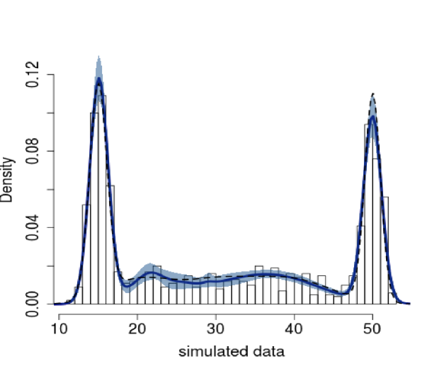
Figure 2: Density estimate for case A5: posterior mean (line), $90\%$ pointwise credibility intervals (shadowed area), true density (dashed) and the histogram of simulated data.

Here, we focus on density estimation: all the tests provide similar estimates, quite faithful to the true density.

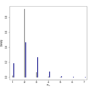
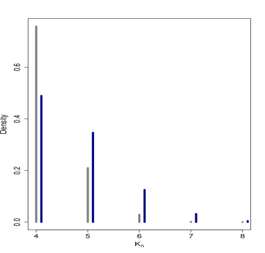
Figure 3: Prior (a) and posterior (b) distributions of the number $K_{n}$ of groups for test A1 (gray) and A5 (blue).

Figure 2 shows density estimate and pointwise $90\%$ credibility intervals for case A5; the true density is superimposed as dashed line. Figure 3 (a) and (b) display prior and posterior distributions, respectively, of the number $K_{n}$ of groups, i.e. the number of unique values among $(\theta_{1},\ldots,\theta_{n})$ in (19) under two sets of hyperparameters, A1, representing an approximation of the DPM model, and A5, where the parameter $\omega$ is nearly 1. From Figure 3 it is clear that A5 is more flexible than A1: for case A5, a priori the variance of $K_{n}$ is larger, and, on the other hand, the posterior probability mass in 5 (the true value) is larger.

In order to compare different priors, we take into account five different predictive goodness-of-fit indexes: $(i)$ the sum of squared errors (SSE) , i.e. the sum of the squared differences between the $y_{i}$ and the predictive mean $\mathbb{E}(Y_{i}|data)$ (yes, we are using data twice!); $(ii)$ the sum of standardized absolute errors (SSAE), given by the sum of the standardized error $|y_{i}-\mathbb{E}(Y_{i}|data)|/\sqrt{\operatorname{Var}(Y_{i}|data)}$; $(iii)$ log-pseudo marginal likelihood (LPML), quite standard in the Bayesian literature, defined as the sum of $\log(CPO_{i})$, where $CPO_{i}$ is the conditional predictive ordinate of $y_{i}$, the value of the predictive distribution evaluated at $y_{i}$, conditioning on the training sample given by all data except $y_{i}$. The last two indexes, $(iv)$ $WAIC_{1}$ and $(v)$ $WAIC_{2}$, as denoted here, were proposed in Watanabe (2010) and deeply analyzed in Gelman et al. (2014): they are generalizations of the AIC, adding two types of penalization, both accounting for the “effective number of parameters”. The bias correction in ${WAIC_{1}}$ is similar to the bias correction in the definition of the DIC, while ${WAIC_{2}}$ is the sum of the posterior variances of the conditional density of the data. See Gelman et al. (2014) for their precise definition. Table 1 shows the values of the five indexes for each test: the optimal (according to each index) tests are highlighted in bold for the experiments $(A)$, $(B)$ and $(C)$. It is apparent that the different tests provide similar values of the indexes, but SSE, indicating that, from a predictive viewpoint, there are no significant differences among the priors. However, especially when the value of $\kappa$ is small, i.e. in all tests $A$ and $B$, a model with a smaller $\omega$ tends to outperform the Dirichlet process case (approximately, when $\omega=100$). On the other hand, the SSE index shows quite different values among the tests: it is well-known that this is a index favoring complex models and leading to better results when data are over-fitted. Therefore, tests with an higher value of $\kappa$ are always preferable according to this criterion.

Table 1: Predictive goodness-of-fit indexes for the simulated dataset.

Test	$\omega$	$\kappa$	SSE	SSAE	WAIC1	WAIC2	LPML
A1	100	0.06	6346.59	811.16	-3312.44	-3312.55	-3312.55
A2	4	0.09	5812.86	810.43	-3312.33	-3312.42	-3312.43
A3	2	0.1	6089.19	810.99	-3312.38	-3312.47	-3312.48
A4	1.33	0.11	6498.23	811.29	-3312.54	-3312.62	-3312.63
A5	1.05	0.11	5725.18	810.39	-3312.27	-3312.36	-3312.36
B1	100	0.43	5184.25	809.61	-3311.95	-3312	-3312.01
B2	4	0.67	5125.41	809.7	-3312.19	-3312.25	-3312.26
B3	2	0.81	4610.39	809.42	-3311.92	-3311.98	-3312
B4	1.33	0.93	4246.43	809.07	-3311.75	-3311.83	-3311.84
B5	1.05	1	4571.09	809.08	-3311.96	-3312.05	-3312.06
C1	100	1.56	3707.5	809.36	-3311.73	-3311.86	-3311.88
C2	4	2.67	2194.1	808.8	-3312.02	-3312.23	-3312.26
C3	2	3.64	1223.86	809.28	-3312.62	-3312.96	-3312.99
C4	1.33	5.29	748.85	808.7	-3313.05	-3313.51	-3313.54
C5	1.05	8.95	685	807.96	-3312.9	-3313.36	-3313.38

We fitted our model also to a real dataset, the Hidalgo stamps data of Wilson (1983) consisting of $n=485$ measurements of stamp thickness in millimeters (here multiplied by $10^{3}$). The stamps have been printed between 1872 and 1874 on different paper types, see data histogram in Figure 4. This dataset has been analyzed by different authors in the context of mixture models: see, for instance, Izenman and Sommer (1988), McAuliffe et al. (2006) and Nieto-Barajas (2013).

We report posterior inference for the set of hyperparameters which is most in agreement with our prior belief: the mean distribution is $P_{0}(d\mu,d\sigma^{2})=\mathcal{N}(d\mu;\bar{y}_{n},\sigma^{2}/\kappa_{0})\times inv-gamma(d\sigma^{2};a,b)$ as before, and $\kappa_{0}=0.005$, $a=2$ and $b=0.1$. The approximation parameter $\varepsilon$ of the $\varepsilon$-NB$(\omega,\kappa P_{0})$ random measure is fixed to $10^{-6}$; on the other hand, in order to set parameters $\omega$ and $\kappa$, we argue as follows: $\omega$ ranges in $\{1.05,5,10,1000\}$ and we choose the mass parameter $\kappa$ such that the prior mean of the number of clusters, i.e. $\mathbb{E}(K_{n})$, is the desired one. As noted in Section 6.1, a closed form of the prior distribution of $K_{n}$ is not available, so we resort to Monte Carlo simulation to estimate it. Table 2 shows the four couples of $(\omega,\kappa)$ yielding $\mathbb{E}(K_{n})=7$: indeed, according to Ishwaran and James (2002) and McAuliffe et al. (2006) and references therein, there are at least 7 different groups (but the true number is unknown), corresponding to the number of types of paper used. For an in-depth discussion about the appropriate number of groups in Hidalgo stamps data, we refer the reader to Basford et al. (1997). Table 2 also reports prior standard deviations of $K_{n}$: even if the a-priori differences are small, the posteriors appear to be quite different among the 4 tests. All the posterior distributions on $K_{n}$ support the conjecture of at least seven distinct modes in the data; in particular, Figure 4 (b) displays the posterior distribution of $K_{n}$ for Test 4. A modest amount of mass is given to less than 7 groups, and the mode is in 11. Even Test 1, corresponding to the Dirichlet process case, does not give mass to less than 7 groups, where 9 is the mode. Density estimates seem pretty good; an example is given in Figure 4 (a), with 90$\%$ credibility band for Test 4.

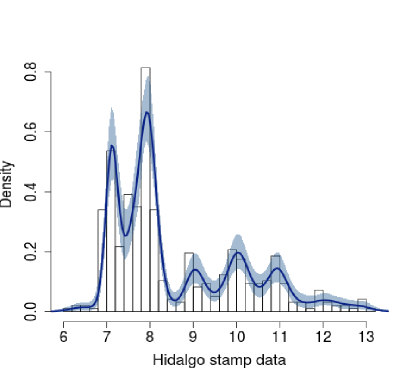
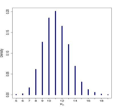
Figure 4: Posterior inference for the Hidalgo stamp data for Test 4: histogram of the data, density estimate and 90$\%$ pointwise credibility intervals (a); posterior distribution of $K_{n}$ (b).

As in the simulated data example, some predictive goodness-of-fit indexes are reported in Table 2: the optimal value for each index is indicated in bold. The SSE is significantly lower when $\omega$ is small, thus suggesting a greater flexibility of the model with small values of $\omega$. The other indexes assume the optimal value in Test 4 as well, even if those values are similar along the tests.

Table 2: Predictive goodness-of-fit indexes for the Hidalgo stamps data.

Test	$\omega$	$\kappa$	$\mathbb{E}(K_{n})$	$sd(K_{n})$	SSE	SSAE	WAIC1	WAIC2	LPML
1	1000	0.98	7	2.04	15.17	384.1	-713.12	-713.96	-714.12
2	10	0.91	7	2.13	12.85	383.51	-713.22	-714.04	-714.25
3	5	0.92	7	2.18	13.52	383.68	-713.52	-714.3	-714.4
4	1.05	1.02	7	2.32	11.12	383.38	-712.84	-713.66	-714.05

7 Linear dependent NGG mixtures: an application to sports data

Let us consider a regression problem, where the response $Y$ is univariate and continuous, for ease of notation. We model the relationship (in distributional terms) between the vector of covariates $\bm{x}=(x_{1},\dots,x_{p})$ and the response $Y$ through a mixture density, where the mixing measure is a collection $\left\{P_{\bm{x}},\textbf{x}\in\mathcal{X}\right\}$ of $\varepsilon$-NormCRMs, being $\mathcal{X}$ the space of all possible covariates. We follow the same approach as in MacEachern (1999), MacEachern (2000), De Iorio et al. (2009) for the dependent Dirichlet process. We define the dependent $\varepsilon$-NormCRM process $\left\{P_{\bm{x}},{\bm{x}}\in\mathcal{X}\right\}$, conditionally to $\bm{x}$, as:

(28) $$P_{\bm{x}}\stackrel{{\scriptstyle d}}{{=}}\sum_{j=0}^{N_{\varepsilon}}P_{j}\delta_{\bm{\gamma}_{j}(\bm{x})}.$$

The weights $P_{j}$ are the normalized jumps as in (5), while the locations $\gamma_{j}(\bm{x})$, $j=1,2,\ldots$, are independent stochastic processes with index set $\mathcal{X}$ and $P_{0\bm{x}}$ marginal distributions. Model (28) is such that, marginally, $P_{\bm{x}}$ follows a $\varepsilon$-NormCRM process, with parameter $(\rho,\kappa P_{0\bm{x}})$, where $\rho$ is the intensity of a Poisson process on ${\mathbb{R}}^{+}$, $\kappa>0$, and $P_{0\bm{x}}$ is a probability on ${\mathbb{R}}$. Observe that, since $N_{\varepsilon}$ and $P_{j}$ do not depend on $\bm{x}$, (28) is a generalization of the single weights dependent Dirichlet process (see Barrientos et al., 2012, for this terminology). We also assume the functions ${\bm{x}}\mapsto\gamma_{j}({\bm{x}})$ to be continuous.

The dependent $\varepsilon$-NormCRM process in (28) takes into account the vector of covariates $\bm{x}$ only through $\gamma_{j}(\bm{x})$. In particular, when the kernel of the mixture (19) belongs to the exponential family, for each $j$, $\gamma_{j}(\bm{x})=\gamma(\bm{x};\bm{\tau}_{j})$ can be assumed as the link function of a generalized linear model, so that (19) specializes to

(29) $$\begin{split}Y_{i}|\bm{\theta}_{i},\bm{x}_{i}&\stackrel{{\scriptstyle\mathrm{ind}}}{{\sim}}f(\bm{y};\bm{\gamma}(\bm{x}_{i},\bm{\theta}_{i}))\ \ \ i=1,\dots,n\\ \bm{\theta}_{i}|P_{\varepsilon}&\stackrel{{\scriptstyle\mathrm{iid}}}{{\sim}}P_{\varepsilon}\ \ \ i=1,\dots,n\qquad\textrm{ where }P_{\varepsilon}\sim\varepsilon-\text{NormCRM}(\rho,\kappa P_{0}).\end{split}$$

This last formulation is convenient because it facilitates parameters interpretation as well as numerical posterior computation.

We analyze the Australian Institute of Sport (AIS) data set (Cook and Weisberg, 1994), which consists of 11 physical measurements on 202 athletes (100 females and 102 males). Here the response is the lean body mass (lbm), while three covariates are considered, the red cell count (rcc), the height in cm (Ht) and the weight in Kg (Wt). The data set is contained in the R package DPpackage (Jara et al., 2011). The actual model (29) we consider here is when $f(\cdot;\mu,\eta^{2})$ is the Gaussian distribution with $\mu$ mean and $\eta^{2}$ variance; moreover, $\mu=\gamma({\bm{x}},\bm{\theta})={\bm{x}}^{t}\bm{\theta}$, and the mixing measure $P_{\varepsilon}$ is the $\varepsilon$-NGG$(\kappa,\sigma,P_{0})$, as introduced in Argiento et al. (2015). We have considered two cases, when mixing the variance $\eta^{2}$ with respect to the NGG process or when the variance $\eta^{2}$ is given a parametric density; in both cases, by linearity of the mean ${\bm{x}}^{t}\bm{\theta}$, the model (here called linear dependent NGG mixture) can be interpreted as a NGG process mixture model, and inference can be achieved via an algorithm similar to that in Section 5. We set $\varepsilon=10^{-6}$, $\sigma\in\{0.001,0.125,0.25\}$, and $\kappa$ such that $\mathbb{E}(K_{n})\simeq 5$ or 10. When the variance $\eta^{2}$ is included in the location points of the $\varepsilon$-NGG process, then $P_{0}$ is $\mathcal{N}_{4}({\bm{b}}_{0},\Sigma_{0})\times$inv-gamma$(\nu_{0}/2,\nu_{0}\eta_{0}^{2}/2)$; on the other hand, when $\eta^{2}$ is given a parametric density, then $\eta^{2}\sim$inv-gamma$(\nu_{0}/2,\nu_{0}\eta_{0}^{2}/2)$. We fixed hyperparameters in agreement with the least squares estimate: ${\bm{b}}_{0}=(-50,5,0,0)$, $\Sigma_{0}=diag(100,10,10,10)$, $\nu_{0}=4$, $\eta_{0}^{2}=1$. For all the experiments, we computed the posterior of the number of groups, the predictive densities at different values of the covariate vectors and the cluster estimate via posterior maximization of Binder’s loss function (see Lau and Green, 2007). Moreover, we compared the different prior settings computing predictive goodness-of-fit tools, specifically log pseudo-marginal likelihood (LPML) and the sum of squared errors (SSE), as introduced in Section 6.2. The minimum value of SSE, among our experiments, was achieved when $\eta^{2}$ is included in the location of the $\varepsilon$-NGG process, $\sigma=0.001$ and $\kappa=0.8$ so that $\mathbb{E}(K_{n})\simeq 5$. On the other hand, the optimal LPML was achieved when $\sigma=0.125$, $\kappa=0.4$, and $\mathbb{E}(K_{n})\simeq 5$.

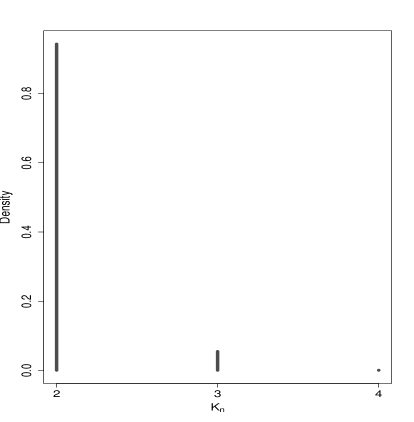
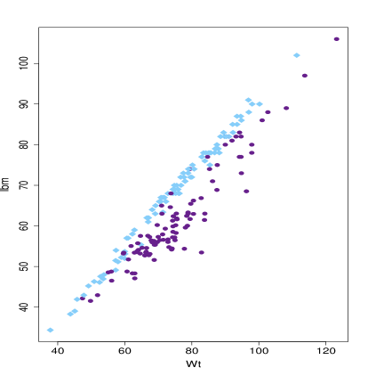
Figure 5: Posterior distributions of the number $K_{n}$ of groups (a) and cluster estimate (b) under the linear dependent $\varepsilon-$NGG mixture.

Posterior of $K_{n}$ and cluster estimate under this last hyperparameter setting are in Figure 5 ($(a)$ and ($b$), respectively); in particular the cluster estimate is displayed in the scatterplot of the Wt vs lbm. In spite of the vague prior, the posterior of $K_{n}$ is almost degenerate on $2$, giving evidence to the existence of two linear relationships between lbm and Wt.

Finally, Figure 6 displays predictive densities and 95% credibility bands for 3 athletes, a female (Wt=60, rcc=3.9, Ht=176 and lbm=53.71), and two males (Wt=67.1,113.7, rcc=5.34,5.17, Ht=178.6, 209.4 and lbm=62,97, respectively); the dashed lines are observed values of the response. Depending on the value of the covariate, the distribution shows one or two peaks: this reflects the dependence of the grouping of the data on the value of $\mathbf{x}$.

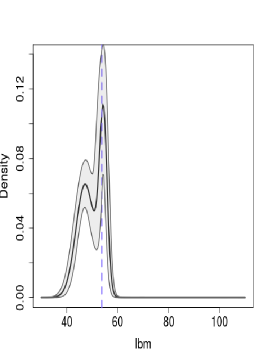
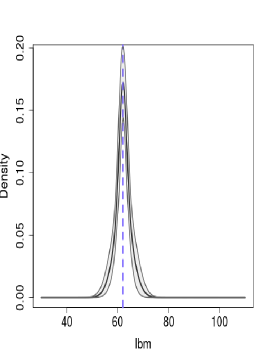
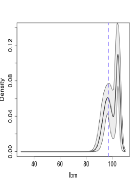
Figure 6: Predictive distributions of lbm for three different athletes: Wt=60, rcc=3.9, Ht=176 (a), Wt=67.1, rcc=5.34, Ht=178.6 (b), Wt=113.7, rcc=5.17, Ht=209.4 (c). The shaded area is the predictive 95% pointwise credible interval, while the dashed vertical line denotes the observed value of the response.

This figure highlights the versatility of nonparametric priors in a linear regression setting with respect to the customary parametric priors: indeed, the model is able to capture in detail the behavior of the data, even when several clusters are present.

8 Discussion

We have proposed a new model for density and cluster estimation in the Bayesian nonparametric framework. In particular, a finite dimensional process, the $\varepsilon$-NormCRM, has been defined, which converges in distribution to the corresponding normalized completely random measure, when $\varepsilon$ tends to 0. Here, the $\varepsilon$-NormCRM is the mixing measure in a mixture model. In this paper we have fixed $\varepsilon$ very small, but we could choose a prior for $\varepsilon$ and include this parameter into the Gibbs sampler scheme. Among the achievements of the work, we have generalized all the theoretical results obtained in the special case of NGG in Argiento et al. (2015), including the expression of the eppf for an $\varepsilon$-NormCRM process, its convergence to the corresponding eppf of the nonparametric underlying process and the posterior characterization of $P_{\varepsilon}$. Moreover, we have provided a general Gibbs Sampler scheme to sample from the posterior of the mixture model. To show the performance of our algorithm and the flexibility of the model, we have illustrated two examples via normalized completely random measure mixtures: in the first application, we have introduced a new normalized completely random measure, named normalized Bessel random measure; we have studied its theoretical properties and used it as the mixing measure in a model to fit simulated and real datasets. The second example we have dealt with is a linear dependent $\varepsilon$-NGG mixture, where the dependence lies on the support points of the mixing random probability, to fit a well known dataset. Current and future research is devoted on the use of our approximation on more complex dependence structures.

APPENDIX: DETAILS ON FULL-CONDITIONALS FOR THE GIBBS SAMPLER

Here, we provide some details about Step 3 of the Gibbs Sampler in Section 5. As far as Step 3a is concerned, the full-conditional $\mathcal{L}(\varepsilon|u,\bm{\theta})$ is obtained integrating out $N_{\varepsilon}$ (or equivalently $N_{na}$) from the law $\mathcal{L}(N_{\varepsilon},u,\bm{\theta})$, as follows:

$$\begin{split}\mathcal{L}(\varepsilon|u,\bm{\theta},\bm{Y})&\propto\sum_{N_{na}=0}^{+\infty}\mathcal{L}(N_{na},\varepsilon,u,\bm{\theta},\bm{Y})\\ &=\sum_{N_{na}=0}^{+\infty}\pi(\varepsilon)e^{-\Lambda_{\varepsilon}}\dfrac{\Lambda_{\varepsilon,u}^{N_{na}}}{\Lambda_{\varepsilon}}\dfrac{(N_{na}+k)}{N_{na}!}\prod_{i=1}^{k}\int_{\varepsilon}^{+\infty}\kappa s^{n_{i}}\mathrm{e}^{-us}\rho(s)ds\\ &=\left(\prod_{i=1}^{k}\int_{\varepsilon}^{+\infty}\kappa s^{n_{i}}\mathrm{e}^{-us}\rho(s)ds\right)e^{\Lambda_{\varepsilon,u}-\Lambda_{\varepsilon}}\dfrac{\Lambda_{\varepsilon,u}+k}{\Lambda_{\varepsilon}}\pi(\varepsilon)=f_{\varepsilon}(u;n_{1},\dots,n_{k})\pi(\varepsilon),\end{split}$$

where we used the identity $\sum_{N_{na}=0}^{+\infty}\Lambda_{\varepsilon,u}^{N_{na}}(N_{na}+k)/(N_{na}!)$ $=e^{\Lambda_{\varepsilon,u}}(\Lambda_{\varepsilon,u}+k)$, as previously noted. Moreover, $f_{\varepsilon}(u;n_{1},\dots,n_{k})$ is defined in (11). This step depends explicitly on the expression of $\rho(s)$.

Step 3.b consists in sampling from $\mathcal{L}(P_{\varepsilon}|\varepsilon,u,\bm{\theta})$ and has already been described in the proof of Propositùion 4. However, for a complete outline of the algorithm, we list the full-conditionals resulting into Step 3b:

1. $\mathcal{L}(N_{na}|\varepsilon,\bm{Y},u,\bm{\theta})=\dfrac{\Lambda_{\varepsilon u}}{\Lambda_{\varepsilon u}+k}\mathcal{P}_{1}(\Lambda_{\varepsilon u})+\dfrac{k}{\Lambda_{\varepsilon u}+k}\mathcal{P}_{0}(\Lambda_{\varepsilon u})$; this is formula (14).

2. Non-allocated jumps: iid from $\mathcal{L}(J_{j})\propto e^{-uJ_{j}}\rho(J_{j})\mathbbm{1}_{(\varepsilon,\infty)}(J_{j}),$ $j=1,\dots,N_{na}$; see the second factor of the last expression in (15).

3. Allocated jumps: iid from $\mathcal{L}(J_{l^{*}_{i}})\propto J_{l^{*}_{i}}^{n_{i}}e^{-uJ_{l^{*}_{i}}}\rho(J_{l^{*}_{i}})\mathbbm{1}_{(\varepsilon,\infty)}(J_{l^{*}_{i}})$, $i=1,\dots,k$; see the first factor of the last expression in (15).

4. Non-allocated points of support: iid from $P_{0}$; see (20).

5. Allocated points of support: iid from $\mathcal{L}(\tau^{*}_{i})\propto\{\prod_{j\in C_{i}}k(X_{j};\tau_{i})\}P_{0}(\tau_{i})$, $i=1,\dots,k$; see (20).

References

- Antoniak (1974) Antoniak, C. E. (1974). Mixtures of Dirichlet processes with applications to Bayesian nonparametric problems. The Annals of Statistics 2, 1152–1174.
- Argiento et al. (2015) Argiento, R., I. Bianchini, and A. Guglielmi (2015). A blocked Gibbs sampler for NGG-mixture models via a priori truncation. Statist. Comp. Online First.
- Argiento et al. (2015) Argiento, R., A. Guglielmi, C. Hsiao, F. Ruggeri, and C. Wang (2015). Modelling the association between clusters of SNPs and disease responses. In R. Mitra and P. Mueller (Eds.), Nonparametric Bayesian Methods in Biostatistics and Bioinformatics. Springer.
- Argiento et al. (2010) Argiento, R., A. Guglielmi, and A. Pievatolo (2010). Bayesian density estimation and model selection using nonparametric hierarchical mixtures. Computational Statistics and Data Analysis 54, 816–832.
- Barndorff-Nielsen (2000) Barndorff-Nielsen, O. E. (2000). Probability densities and Lévy densities. University of Aarhus. Centre for Mathematical Physics and Stochastics.
- Barrientos et al. (2012) Barrientos, A. F., A. Jara, F. A. Quintana, et al. (2012). On the support of MacEachern¿s dependent Dirichlet processes and extensions. Bayesian Analysis 7(2), 277–310.
- Barrios et al. (2013) Barrios, E., A. Lijoi, L. E. Nieto-Barajas, and I. Prünster (2013). Modeling with normalized random measure mixture models. Statistical Science 28, 313–334.
- Basford et al. (1997) Basford, K., G. McLachlan, and M. York (1997). Modelling the distribution of stamp paper thickness via finite normal mixtures: The 1872 Hidalgo stamp issue of Mexico revisited. Journal of Applied Statistics 24(2), 169–180.
- Cook and Weisberg (1994) Cook, R. D. and S. Weisberg (1994). An introduction to regression graphics. John Wiley & Sons.
- De Iorio et al. (2009) De Iorio, M., W. O. Johnson, P. Müller, and G. L. Rosner (2009). Bayesian nonparametric nonproportional hazards survival modeling. Biometrics 65(3), 762–771.
- Erdélyi et al. (1953) Erdélyi, A., W. Magnus, F. Oberhettinger, F. G. Tricomi, and H. Bateman (1953). Higher transcendental functions, Volume 2. McGraw-Hill New York.
- Escobar and West (1995) Escobar, M. and M. West (1995). Bayesian density estimation and inference using mixtures. J. Amer. Statist. Assoc. 90, 577–588.
- Favaro and Teh (2013) Favaro, S. and Y. Teh (2013). MCMC for normalized random measure mixture models. Statistical Science 28(3), 335–359.
- Feller (1971) Feller, W. (1971). An introduction to probability theory and its Applications, vol. II (Second Edition ed.). John Wiley, New York.
- Foti and Williamson (2015) Foti, N. and S. Williamson (2015). A survey of non-exchangeable priors for Bayesian nonparametric models. IEEE Transactions on pattern Analysis and Machine Intelligence 37, 359–371.
- Gelman et al. (2014) Gelman, A., J. Hwang, and A. Vehtari (2014). Understanding predictive information criteria for Bayesian models. Statistics and Computing 24(6), 997–1016.
- Gradshteyn and Ryzhik (2007) Gradshteyn, I. and L. Ryzhik (2007). Table of integrals, series, and products - Seventh Edition (Sixth ed.). San Diego (USA): Academic Press.
- Griffin and Walker (2011) Griffin, J. and S. G. Walker (2011). Posterior simulation of normalized random measure mixtures. Journal of Computational and Graphical Statistics 20, 241–259.
- Griffin (2013) Griffin, J. E. (2013). An adaptive truncation method for inference in Bayesian nonparametric models. arXiv preprint arXiv:1308.2045.
- Ishwaran and James (2001) Ishwaran, H. and L. James (2001). Gibbs sampling methods for stick-breaking priors. J. Amer. Statist. Assoc. 96, 161–173.
- Ishwaran and James (2002) Ishwaran, H. and L. F. James (2002). Approximate Dirichlet process computing in finite normal mixtures. Journal of computational and graphical statistics 11(3).
- Izenman and Sommer (1988) Izenman, A. J. and C. J. Sommer (1988). Philatelic mixtures and multimodal densities. Journal of the American Statistical association 83(404), 941–953.
- James et al. (2009) James, L., A. Lijoi, and I. Prünster (2009). Posterior analysis for normalized random measures with independent increments. Scand. J. Statist. 36, 76–97.
- Jara et al. (2011) Jara, A., T. E. Hanson, F. A. Quintana, P. Müller, and G. L. Rosner (2011). DPpackage: Bayesian semi-and nonparametric modeling in R. Journal of statistical software 40(5), 1.
- Kingman (1975) Kingman, J. F. C. (1975). Random discrete distributions. Journal of the Royal Statistical Society 37(1), 1–22.
- Kingman (1993) Kingman, J. F. C. (1993). Poisson processes, Volume 3. Oxford university press.
- Lau and Green (2007) Lau, J. W. and P. J. Green (2007). Bayesian model based clustering procedures. Journal of Computational and Graphical Statistics 16, 526–558.
- Lijoi et al. (2005) Lijoi, A., R. H. Mena, and I. Prünster (2005). Hierarchical mixture modeling with normalized inverse-gaussian priors. Journal of the American Statistical Association 100(472), 1278–1291.
- Lo (1984) Lo, A. J. (1984). On a class of Bayesian nonparametric estimates: I. density estimates. The Annals of Statistics 1.
- Lomelí et al. (2014) Lomelí, M., S. Favaro, and Y. W. Teh (2014). A marginal sampler for -stable Poisson-Kingman mixture models. arXiv preprint arXiv:1407.4211.
- MacEachern (1999) MacEachern, S. N. (1999). Dependent nonparametric processes. In ASA proceedings of the section on Bayesian statistical science, pp. 50–55.
- MacEachern (2000) MacEachern, S. N. (2000). Dependent Dirichlet processes. Technical report, Department of Statistics, The Ohio State University.
- McAuliffe et al. (2006) McAuliffe, J. D., D. M. Blei, and M. I. Jordan (2006). Nonparametric empirical Bayes for the Dirichlet process mixture model. Statistics and Computing 16(1), 5–14.
- Nieto-Barajas (2013) Nieto-Barajas, L. E. (2013). Lévy-driven processes in bayesian nonparametric inference. Bol. Soc. Mat. Mexicana (3) 19.
- Pitman (1996) Pitman, J. (1996). Some developments of the Blackwell-Macqueen urn scheme. In T. S. Ferguson, L. S. Shapley, and M. J. B. (Eds.), Statistics, Probability and Game Theory: Papers in Honor of David Blackwell, Volume 30 of IMS Lecture Notes-Monograph Series, pp. 245–267. Hayward (USA): Institute of Mathematical Statistics.
- Pitman (2003) Pitman, J. (2003). Poisson-Kingman partitions. In Science and Statistics: a Festschrift for Terry Speed, Volume 40 of IMS Lecture Notes-Monograph Series, pp. 1–34. Hayward (USA): Institute of Mathematical Statistics.
- Pitman (2006) Pitman, J. (2006). Combinatorial Stochastic Processes. LNM n. 1875. New York: Springer.
- Regazzini et al. (2003) Regazzini, E., A. Lijoi, and I. Prünster (2003). Distributional results for means of random measures with independent increments. The Annals of Statistics 31, 560–585.
- Watanabe (2010) Watanabe, S. (2010). Asymptotic equivalence of Bayes cross validation and widely applicable information criterion in singular learning theory. The Journal of Machine Learning Research 11, 3571–3594.
- Wilson (1983) Wilson, I. (1983). Add a new dimension to your philately. The American Philatelist 97, 342–349.