Lévy flights and nonhomogenous memory effects: relaxation to a stationary state

Abstract

The non-Markovian stochastic dynamics involving Lévy flights and a potential in the form of a harmonic and non-linear oscillator is discussed. The subordination technique is applied and the memory effects, which are nonhomogeneous, are taken into account by a position-dependent subordinator. In the non-linear case, the asymptotic stationary states are found. The relaxation pattern to the stationary state is derived for the quadratic potential: the density decays like a linear combination of the Mittag-Leffler functions. It is demonstrated that in the latter case the density distribution satisfies a fractional Fokker-Planck equation. The densities for the non-linear oscillator reveal a complex picture, qualitatively dependent on the potential strength, and the relaxation pattern is exponential at large time.

I Introduction

The presence of long distribution tails in stochastic systems means a qualitatively different picture than a familiar Gaussian process. In particular, the variance of the process value $x$ diverges and the ordinary central limit theorem does not apply. Instead of the normal distribution, the power-law form of the asymptotic density distribution, $|x|^{-\alpha-1}$ ($0<\alpha<2$), emerges. Processes characterised by such tails are stable and called Lévy flights. They are typical for complex systems and frequently observed in many areas of science shles ; barn . Processes involving Lévy flights are well suited to describe phenomena far from equilibrium. Dynamics of a particle subjected to the Lévy stable noise can be described by a Langevin equation,

$$dx(t)=-\frac{\partial}{\partial x}V(x)dt+\eta(dt),$$ (1)

where $V(x)$ is a potential and the increments $\eta(dt)$ obey the Lévy stable statistics with the stability index $\alpha$. Solution of the corresponding Fokker-Planck equation is simple for the linear case – when $V(x)=$const, $\propto x$ or $\propto x^{2}$ – and the resulting density reveals the same statistics as the driving noise jes . That equation, in the presence of the Lévy flights determined by a stability index $\alpha$, contains a fractional derivative defined by a Fourier transform old ,

$$\frac{\partial^{\alpha}}{\partial|x|^{\alpha}}f(x)={\cal F}^{-1}[-|k|^{\alpha}{\widetilde{f}}(k)].$$ (2)

For the quadratic potential, the system converges with time to a stationary state. The stationary solutions in the asymptotic limit have been also found for strongly nonlinear systems, $V(x)\propto x^{\gamma}$ ($\gamma>2$), and the steep slope of the potential modifies the distribution making the variance finite che ; che1 . This analysis was generalised to a two-dimensional problem szcz and to systems driven by a multiplicative noise sro10 ; the spectral analysis was performed for transport in an inhomogeneous medium kaz .

The above approach is Markovian (Eq.(1) is local in time) and does not take into account memory effects emerging in complex tak and disordered systems bou where, as a result of traps and faults, the particle experiences periods of long rests. Then the process can be formalised by a jump-size and waiting-time distribution in the framework of the continuous time random walk (CTRW) met . The problem without any potential is well known: the variance – existing for the Gaussian case – rises slower than linearly, which means a subdiffusion, and the characteristic function of the density distribution decays according to the Mittag-Leffler pattern hau . The diffusive behaviour for which the variance rises with time slower or faster than linearly is often called an anomalous transport, in contrast to a normal diffusion. Processes characterised by the anomalous transport – e.g. the flow in porous media where fractional space derivatives model large motions through highly conductive layers or fractures while fractional time derivatives describe motionless particles meer – can be conveniently handled by the subordination procedure sok ; bar1 ; pir . In that description, the Markovian dynamics proceeds in an operational time and is given by Eq.(1) (a subordinated process), whereas the memory effects are modelled by another Langevin equation for the physical time which is a non-decreasing random variable, determined by a one-sided density distribution $\xi$ (a subordinator). In the presence of a potential, the process (1) has a stationary limit and the subordinator determines a relaxation to that stationary state. Long tails of the waiting-time distribution mean a deviation from the exponential Debye relaxation. Non-exponential forms of the relaxation are common in complex systems: viscoelastic materials, synthetic polymers and biopolymers glo . They emerge in supercooled liquids near the glass transition temperature and in amorphous polymers rich ; a typical decay form of the relaxation processes is a Mittag-Leffler function (Cole-Cole) hil . Diversity of systems exhibiting the non-exponential relaxation traces back to the universality present in complex systems: the empirical relaxation laws reflect a behaviour which is independent of the details of examined systems jon . From that point of view, the non-exponential relaxation can be understood as a result of a strong interaction between diverse elementary units.

In a nonhomogeneous medium, one can expect that the waiting time depends on the position. The corresponding CTRW description is coupled met ; its Markovian version contains the waiting-time distribution in a Poissonian form, characterised by a variable jumping rate kam , and resolves itself to a Fokker-Planck equation with a multiplicative noise sro06 . In the disordered systems, many forms of the disorder may emerge bou and the dynamics becomes complicated if one assumes that the trap positions slowly evolve with time (a quenched disorder), then the successive trapping times are correlated. The position-dependence of memory effects can be taken into account by applying a subordination technique and such a model has been recently proposed sro14 . One can expect that a large density of traps or regular structures in the phase space the trajectories stick to invoke a long resting time at specific regions. The subordination approach sro14 takes into account that position-dependence by introducing a variable intensity of the random generator of the physical time, given by a non-negative function $g(x)$. Then Eq.(1) describes the subordinated process and the dynamics is defined by the following set of equations,

$$dx(\tau) = F_{d}(x)d\tau+\eta(d\tau)$$

$$dt(\tau) = g(x)\xi(d\tau),$$ (3)

where the increments $\eta(dt)$ and $\xi(dt)$ obey the Lévy stable statistics with the stability indexes $0<\alpha<2$ and $0<\beta<1$, respectively. The process $t(\tau)$ is non-decreasing and biased by the medium properties: if, in particular, $g(x)$ is large, the particle stays at $x$ for a relatively long time, compared to the region where $g(x)$ is small. Eq.(I) can be approximated by an ordinary subordination process if we decouple the random and the position-dependent ingredient; this can be accomplished by a two-step procedure sro14 . First, let us assume for the moment that $\xi$ is given by a one-sided density with finite moments (e.g. an exponential), approximate $\xi(d\tau)$ by the average, $\langle\xi\rangle d\tau$, and evaluate the operational time increment, $\Delta\tau=(\langle\xi\rangle g(x))^{-1}\Delta t$. Since the first equation (I) can be discretized as $\Delta x=F_{d}(x)\Delta\tau+\Delta\eta\Delta\tau^{1/\alpha}$, the system (I), after inserting $\Delta\tau$, resolves itself to the Langevin equation with a multiplicative noise in the Itô interpretation which defines a Markovian process. The above equation incorporates the spatial distribution of traps but neglects the memory effects which are important if $\beta<1$. Then, as a second step, we take into account those effects subordinating the Markovian process to the random time determined by $\beta<1$. The final set of equations reads,

$$dx(\tau) = F_{d}(x)\nu(x)d\tau+\nu(x)^{1/\alpha}\eta(d\tau)$$

$$dt(\tau) = \xi(d\tau),$$ (4)

where $\nu(x)=[\langle\xi\rangle g(x)]^{-1}$; we assume in the following $\langle\xi\rangle=1$. The process described by Eq.(I) was studied for $F_{d}=0$ sro14 : it corresponds to a Markovian CTRW with a variable jumping rate, subordinated to a random time, and resolves itself to a fractional Fokker-Planck equation with a variable diffusion coefficient. The system (I) is used, for example, to describe such transport phenomena as advection, molecular diffusion and hydrodynamic dispersion, where the first equation (I) is related to the advection-dispersion equation whereas the subordination accounts for memory berk12 .

In the presence of an external potential, Eq.(1) predicts a convergence to a stationary density distribution. However, the stationary state is difficult to derive and known in its exact form only for few potentials che . All the more difficult is a problem of the relaxation to that state and the time-dependent solutions are unknown even for the Markovian case. It is unclear, in particular, whether the Mittag-Leffler pattern is still valid when a process with a nonlinear deterministic force is subordinated to the random time. In the present paper, we address that relaxation problem and consider a more general case of the position-dependent memory. We find expressions for the asymptotic stationary density for the potential in a power-law form and derive the density for the subordinated process, as a function of the operational time, for a quadratic potential (Sec.II). Sec.III is devoted to the time-dependent solutions of Eq.(I), (I) where the relaxation function is derived and the influence of the nonhomogeneity effects on the decay rate of the density is discussed.

II Stationary states and the subordinated process

We consider a stochastic system under the influence of an non-linear deterministic force,

$$F_{d}=-\lambda|x|^{\bar{\gamma}}\hbox{sign}(x),$$ (5)

where $\lambda\geq 0$ and $\bar{\gamma}=$const. This form of the stimulation is a natural generalisation of an ordinary harmonic oscillator and often discussed in connection with the chaotic dynamics che2 . Hence the first equation (I) takes the form,

$$dx(\tau)=-\lambda|x|^{\bar{\gamma}}\nu(x)\hbox{sign}(x)d\tau+\nu(x)^{1/\alpha}\eta(d\tau),$$ (6)

and corresponds to a Fokker-Planck equation sch ,

$$\frac{\partial p_{0}(x,\tau)}{\partial\tau}=\lambda\frac{\partial}{\partial x}[|x|^{\bar{\gamma}}\nu(x)\hbox{sign}(x)p_{0}(x,\tau)]+\frac{\partial^{\alpha}[\nu(x)p_{0}(x,\tau)]}{\partial|x|^{\alpha}},$$ (7)

where the fractional derivative is defined by Eq.(2). The equation for the characteristic function reads

$$\frac{\partial}{\partial\tau}{\widetilde{p}_{0}}(k,\tau)=-\lambda k\frac{\partial}{\partial k}{\cal F}[|x|^{\bar{\gamma}-1}\nu(x)p_{0}(x,\tau)]-|k|^{\alpha}{\cal F}[\nu(x)p_{0}(x,\tau)].$$ (8)

Eq.(8) cannot be analytically solved, in general, and presence of the multiplicative factor $\nu(x)$ in the last term poses the main difficulty. We restrict our considerations to the asymptotic regime in positions, which corresponds to small wave numbers, and derive a stationary solution. Due to the factor $|k|^{\alpha}$ in the last term of Eq.(8), the leading term in the solution is of the order $|k|^{\alpha}$ implying the asymptotic solution in a scaling form,

$$p_{0}(x,\tau)=a(\tau)p_{0}(a(\tau)x)=a(\tau)^{-\bar{\alpha}}|x|^{-\bar{\alpha}-1},$$ (9)

where $\bar{\alpha}=$const; the above solution is valid if $0<\bar{\alpha}<2$. Moreover, it is sufficient to keep only the lowest term, $k^{0}$, in the $k-$expansion of the Fourier transform argument and the transform resolves itself to the integral

$$\int\nu(x)p_{0}(x,\tau)dx.$$ (10)

For the evaluation of the argument of the first Fourier transform an additional assumption is necessary: we require that the asymptotic form of $g(x)$ is algebraic, $g(x)=|x|^{\theta}$, and that argument reads $a(\tau)^{-\bar{\alpha}}|x|^{\bar{\gamma}-\theta-\bar{\alpha}-2}$ for large $|x|$. The last term in Eq.(8), in turn, follows from the integral (10),

$$-|k|^{\alpha}{\cal F}[\nu(x)p_{0}(x,\tau)]=-|k|^{\alpha}\langle\nu(x)\rangle(\tau),$$ (11)

and this expression is valid for any time. Now, we take the limit of large time and look for the stationary solution: $p_{0}(x,\tau\to\infty)=p_{0}^{(s)}(x)$ and $a(\tau\to\infty)=a_{s}$. In that limit, the first transform on the rhs of Eq.(8) reads

$$f(k)=N^{-1}{\cal F}[Na_{s}^{-\bar{\alpha}}|x|^{-\delta-1}],$$ (12)

where $N=\langle|x|^{\bar{\gamma}-1}\nu(x)\rangle^{-1}$ and $\delta=-\bar{\gamma}+\theta+\bar{\alpha}+1$ ($0<\delta<2$). The transform argument is normalised to unity and the transform itself can be simply evaluated up to the first order in $k$ by means of the following lemma gor . If $W(x)$ is a normalised and symmetric density distribution and $\int_{x}^{\infty}dW(x^{\prime})\sim b\alpha^{-1}x^{-\alpha}$ for $x\to\infty$ ($b>0$), then $1-\widetilde{W}(k)\sim bc|k|^{\alpha}$ for $k\to 0$, where

$$c=\frac{\pi}{\Gamma(\alpha+1)\sin(\alpha\pi/2)}.$$ (13)

Application of the above lemma to the present problem yields $f(k)=N^{-1}-ca_{s}^{-\bar{\alpha}}|k|^{\delta}$ and inserting of the evaluated expressions to Eq.(8) produces Fourier transform from the stationary density which contains terms corresponding to $|k|^{\alpha}$ and $|k|^{\delta}$. The equation is satisfied for $\delta=\alpha$ and the parameter $\bar{\alpha}$ is determined: $\bar{\alpha}=\alpha+\gamma-1$, where $\gamma=\bar{\gamma}-\theta$. Moreover, we obtain

$$a_{s}=\left[\frac{\lambda\pi}{\langle\nu(x)\rangle\Gamma(\alpha)\sin(\alpha\pi/2)}\right]^{1/\bar{\alpha}}$$ (14)

and the final asymptotic solution follows from Eq.(9),

$$p_{0}^{(s)}(x)=\frac{\langle\nu(x)\rangle}{\lambda\pi}\Gamma(\alpha)\sin(\alpha\pi/2)|x|^{-\alpha-\gamma}.$$ (15)

The above solution exists if $\bar{\gamma}$ satisfies some conditions: it is normalisable for $\bar{\gamma}>1-\alpha+\theta$ and $\langle\nu(x)\rangle$ is finite for $\bar{\gamma}>1-\alpha$. The $x-$dependence of $p_{0}^{(s)}(x)$ is exact for any $\theta$ but $\langle\nu(x)\rangle$ depends on the density at small $|x|$ and cannot be determined without additional assumptions. For $\theta=0$, Eq.(15) is exact in a wide range of $\bar{\gamma}$, including negative values, and the condition $\bar{\gamma}>1-\alpha$ is required to get a stationary solution dyb .

Our aim is to establish how the system under the force field (5) approaches the stationary state (15), i.e. we have to derive the time-dependence of the density $p_{0}(x,\tau)$. Its asymptotic form can be analytically derived for a linear case. From now on, we restrict our analysis to a power-law form of $g(x)$,

$$g(x)=|x|^{\theta}~{}~{}~{}~{}(\theta>-\alpha),$$ (16)

which is well suited to describe diffusion on fractals osh . It is encountered in geology where a power-law distribution of fracture lengths is responsible for transport in a rock pai ; this self-similar structure of a fracture and fault network is characterised by a fractal dimension and determines a pattern of water and steam penetration in the rock taf . The parameter $\theta$ estimates a degree of the memory nonhomogeneity: for $\theta<0$, $g(x)$ is small near the origin which means long waiting times whereas for $\theta>0$ transport is inhibited at large distances. The deterministic force is linear when $\bar{\gamma}=1+\theta$ and Eq.(7) takes the form,

$$\frac{\partial p_{0}(x,\tau)}{\partial\tau}=\lambda\frac{\partial}{\partial x}[xp(x,\tau)]+\frac{\partial^{\alpha}[|x|^{-\theta}p_{0}(x,\tau)]}{\partial|x|^{\alpha}},$$ (17)

that leads, after the Fourier transformation, to the equation

$$\frac{\partial}{\partial\tau}{\widetilde{p}_{0}}(k,\tau)=-\lambda k\frac{\partial}{\partial k}{\widetilde{p}_{0}}(k,\tau)-|k|^{\alpha}{\cal F}[|x|^{-\theta}p_{0}(x,\tau)].$$ (18)

Eq.(17) cannot be exactly solved for arbitrary $x$; we look for a solution in the limit of small $|k|$. It can be represented by a stable distribution but only in a limited range of $\theta$ sro14a . The solution valid for an arbitrary large $\theta$ contains a power-law tail but its shape at small $|x|$ is different from that for the stable distribution sro09a . In this paper, we assume that the solution has a scaling form that, in the asymptotic regime, is defined by the parameter $\alpha$,

$$p_{0}(x,\tau)=a(\tau)p_{0}(a(\tau)x)=a(\tau)^{-\alpha}|x|^{-\alpha-1},$$ (19)

and the validity of a tentative assumption (19) will be verified and the unknown function $a(\tau)$ determined by inserting Eq.(19) to Eq.(18). For that purpose, both Fourier transforms in Eq.(18) have to be evaluated in a limit of small $|k|$. Transform in the last term is given by the integral (10),

$$a(\tau)\int|x|^{-\theta}p_{0}(a(\tau)x)dx=a(\tau)^{\theta}\int|x|^{-\theta}p_{0}(x)dx\equiv a(\tau)^{\theta}h_{0},$$ (20)

where $h_{0}=$const. By the evaluation of the Fourier transform from $p_{0}(x,\tau)$ we apply the same procedure as in Sec.II and obtain

$${\widetilde{p}_{0}}(k,\tau)=1-\frac{a(\tau)^{-\alpha}\pi}{\Gamma(\alpha+1)\sin(\alpha\pi/2)}|k|^{\alpha}.$$ (21)

Inserting the above expression to Eq.(18) produces a differential equation,

$$\dot{a}(\tau)-\lambda a+\frac{h_{0}}{\alpha c}a(\tau)^{\alpha+\theta+1}=0,$$ (22)

which can be solved by separation of the variables:

$$a(\tau)=A\left[1-\hbox{e}^{-\lambda(\alpha+\theta)\tau}\right]^{-1/(\alpha+\theta)};$$ (23)

in this equation, $A=(\alpha\lambda c/h_{0})^{1/(\alpha+\theta)}$ and $c$ is defined by Eq.(13). The final asymptotic solution is given by Eq.(19) and this expression is exact in respect to time- and position-dependence; the constant $h_{0}$ contains details of the solution for all $x$ and cannot be determined by the above procedure. The case $\theta=0$ is exceptional: then Eq.(17) can be solved exactly for arbitrary $x$ and the solution resolves itself to the stable distribution jes .

III Relaxation to stationary states

Stochastic properties of the systems for which particle is subjected to the Gaussian white noise and remains under the influence of an external deterministic force are usually described by the Fokker-Planck equation. The expansion of its solution to the eigenfunctions of the Fokker-Planck operator contains single modes which decay exponentially in time to a stationary state representing a Gibbs-Boltzmann distribution and the temperature is related to the diffusion coefficient by the fluctuation-dissipation theorem met . Generalisation of that equation takes into account the memory effects by introducing a fractional derivative over time (the fractional Fokker-Planck equation). In this generalised description, a different relaxation pattern of the single modes emerges: the decay is governed by the Mittag-Leffler function met and, in the case of the harmonically bound particle, also the variance decays according to that pattern met99 . The Mittag-Leffler relaxation naturally emerges in the subordination technique pir .

The system, relaxation properties of which are analysed in the present paper, is defined by the stochastic equation (I). It includes the random force in a form of the Lévy stable distribution and the non-Markovian nature of the process is taken into account by applying a subordination technique: the process – described in Sec.II and given by $p_{0}(x,\tau)$ – is subordinated to the random time. This time is defined by a one-sided, maximally asymmetric stable Lévy distribution $h^{\prime}(\tau,t)=L_{\beta}(\tau)$, where $0<\beta<1$, which vanishes for $\tau<0$. Since the processes $x(\tau)$ and $\tau(t)$ are statistically independent, the distribution as a function of the physical time is given by the total probability formula,

$$p(x,t)=\int_{0}^{\infty}p_{0}(x,\tau)h(\tau,t)d\tau,$$ (24)

where $h(\tau,t)=\frac{t}{\beta\tau}L_{\beta}(\frac{t}{\tau^{1/\beta}})$ denotes an inverse subordinator pir . In the next subsection, we derive that distribution for the linear case. Note that stationary state is completely determined by the distribution $p_{0}(x,\tau)$, i.e. by the noise type and the potential, whereas the subordinator, as a source of the subdiffusion, influences only the relaxation to that state.

III.1 Linear case

Let us consider the case $\bar{\gamma}=1+\theta$ which condition means that the effective deterministic force in the first equation (I) is linear and the subordinated process is governed by Eq.(17). Note that then the force $F_{d}$ in Eq.(5) may be nonlinear. The density $p(x,t)$ follows from Eq.(24) and can be evaluated by a direct integration. For that purpose, we insert the expression (21) to Eq.(24) and calculate the Fourier and Laplace transform taking into account that the Laplace transform from $h(\tau,t)$ is given by $\bar{h}(\tau,u)=u^{\beta-1}\exp(-\tau u^{\beta})$. This procedure yields

$${\widetilde{p}}(k,u)=\frac{1}{u}-c|k|^{\alpha}u^{\beta-1}\int_{0}^{\infty}a(\tau)^{-\alpha}\hbox{e}^{-\tau u^{\beta}}d\tau$$ (25)

and the expression for $a(\tau)^{-\alpha}$ results from Eq.(23) by applying a direct exponentiation:

$$A^{\alpha}a(\tau)^{-\alpha}=1+\sum_{j=1}^{\infty}\frac{(-1)^{j}}{j!}\hbox{e}^{-\lambda(\alpha+\theta)j\tau}\prod_{i=0}^{j-1}(q-i),$$ (26)

where $q=\alpha/(\alpha+\theta)$. The integration yields the transformed density,

$${\widetilde{p}}(k,u)=\frac{1}{u}-cA^{-\alpha}|k|^{\alpha}\left[\frac{1}{u}+\sum_{j=1}^{\infty}\frac{(-1)^{j}}{j!}\frac{u^{\beta-1}}{u^{\beta}+\lambda(\alpha+\theta)j}\prod_{i=0}^{j-1}(q-i)\right].$$ (27)

The above transform can easily be inverted when we realise that the $u-$dependent term corresponds to a Mittag-Leffler function that is defined by the series

$$E_{\beta}(x)=\sum_{n=0}^{\infty}\frac{x^{n}}{\Gamma(1+\beta n)}$$ (28)

and resolves itself to an ordinary exponential for $\beta=1$. The final expression for the asymptotic form of the density in the Fourier space reads,

$${\widetilde{p}}(k,t)=1-cA^{-\alpha}[1-\chi(t)]|k|^{\alpha},$$ (29)

where a function

$$\chi(t)=-\sum_{j=1}^{\infty}\frac{(-1)^{j}}{j!}E_{\beta}[-\lambda(\alpha+\theta)jt^{\beta}]\prod_{i=0}^{j-1}(q-i),$$ (30)

involving a series of the Mittag-Leffler functions, determines the relaxation to the stationary state and $\chi(\infty)=0$. Inversion of the Fourier transform yields a time-dependence of the asymptotic solution,

$$p(x,t)=A^{-\alpha}[1-\chi(t)]|x|^{-\alpha-1}~{}~{}~{}~{}(|x|\gg 1).$$ (31)

Notice that $\chi(t)$ does not depend on $h_{0}$ and is exact, in contrast to the intensity of $p(x,t)$; the latter quantity depends on the shape of the density at small $|x|$ and is not determined by the present method. The long-time behaviour of the relaxation function $\chi(t)$ agrees with that of the Mittag-Leffler function and then $\chi(t)\propto t^{-\beta}$ but the effective relaxation time may strongly depend on the parameter $\theta$. Fig.1 presents $\chi(t)$ calculated from Eq.(30) for a few values of $\theta$. The Mittag-Leffler function was determined from Eq.(28) for small $t$ and from the expansion

$$E_{\beta}(x)=-\sum_{n=1}^{\infty}\frac{x^{-n}}{\Gamma(1-\beta n)}$$ (32)

for large $t$; the convergence could not be achieved for intermediate values uwa . Despite the same asymptotic form, the relaxation time substantially differs for various $\theta$: it is very large for $\theta<0$.

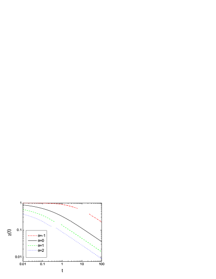
Figure 1: (Colour online) Relaxation function $\chi(t)$ calculated from Eq.(30) for $\alpha=1.5$, $\beta=0.5$, $\lambda=1$ and a few values of $\theta$.

The time-dependent density distribution for a stochastic dynamical system satisfies a Fokker-Planck equation which, in the presence of jumps and/or long waiting times, is fractional. This equation can be derived from the generalised master equation and CTRW met ; it has been applied, in particular, to describe chaotic systems characterised by a hierarchical structure of the trajectories zas . The equation in the latter case possesses, in general, a variable diffusion coefficient. The fractional Fokker-Planck equation has a stochastic representation in a form of equations similar to (I). This has been proved for the homogeneous case with an arbitrary potential mag and that equivalence can be generalised to the nonhomogeneous case. Indeed, we demonstrate in the Appendix A that the function $p(x,t)$, Eq.(31), satisfies the following Fokker-Planck equation,

$$\frac{\partial p(x,t)}{\partial t}={{}_{0}}D_{t}^{1-\beta}\left[\lambda\frac{\partial}{\partial x}[xp(x,t^{\prime})]+\frac{\partial^{\alpha}}{\partial|x|^{\alpha}}(|x|^{-\theta}p(x,t))\right],$$ (33)

where the Riemann-Liouville fractional derivative is defined by the integral operator,

$$_{0}D_{t}^{1-\beta}f(t)=\frac{1}{\Gamma(\beta)}\frac{d}{dt}\int_{0}^{t}dt^{\prime}\frac{f(t^{\prime})}{(t-t^{\prime})^{1-\beta}}.$$ (34)

III.2 Nonlinear case: a numerical analysis

In this subsection, we consider the general case when the effective deterministic force in the first equation (I) is a nonlinear function of $x$ ($\bar{\gamma}\neq 1+\theta$). To evaluate the density $p(x,t)$ from Eq.(24) we need the distribution for the subordinated process, $p_{0}(x,\tau)$, i.e. the solution of Eq.(7). This distribution cannot be found analytically, even for $\theta=0$, if $\gamma=\bar{\gamma}-\theta\neq 1$. Therefore, we must resort to a numerical analysis details of which are presented in Appendix B.

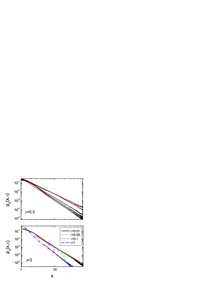
Figure 2: (Colour on line) The time-evolution of the density distribution for the subordinated process corresponding to two values of $\gamma$ and calculated for $\alpha=1.5$ and $\theta=1$ from Eq.(6). The curves in the upper part correspond to $\tau=$0.05, 0.3, 1, 5 and 20 (from bottom to top). The straight red lines mark the dependence $x^{-1-\alpha}$ and $x^{-\alpha-\gamma}$. Averaging was performed over $10^{7}$ trajectories.

First, we consider Eq.(6) to get a qualitative picture of the solutions for various values of $\gamma$. Just a simple analysis of Eq.(6) indicates that the cases $\gamma>1$ and $\gamma<1$ must be different. The particle, initially positioned at $x=0$, is subjected only to the random force at the beginning of the time-evolution since the first term in Eq.(6) can be neglected for $\gamma\geq 0$. Hence the density distribution corresponds to the case without any potential and $p_{0}(x,\tau)\propto|x|^{-\alpha-1}$. However, the density approaches the stationary limit, which is of the form $|x|^{-\alpha-\gamma}$, differently for both cases: the tail becomes steeper ($\gamma>1$) or flatter ($\gamma<1$) during the evolution. The density distributions for those cases are presented, as a function of time, in Fig.2; we assume, from now on, $\lambda=1$. If $\gamma$ is large, the asymptotic distribution, $|x|^{-\alpha-\gamma}$, is visible already at a very short time but restricted to a large distance. The stationary distribution is reached at $\tau=1$ and the curves for the intermediate cases show a widening of the stationary tail. In contrast to this picture, the case $\gamma=0.3$ exhibits a gradual change of the slope for the entire tail and the stationary distribution is reached at $\tau=10$.

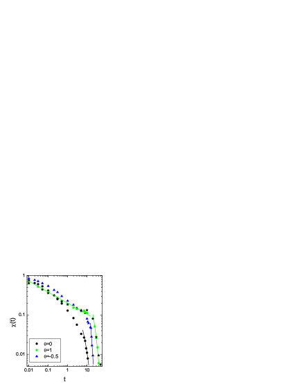
Figure 3: (Colour on line) The relaxation function for $\alpha=1.9$, $\beta=0.5$, $\bar{\gamma}=3$ and three values of $\theta$. The solid lines on the right side mark an exponential, $\exp(-c_{\chi}t)$, with $c_{\chi}=0.33$, 0.4 and 0.14 (from left to right). The solid line on the left side, fitted to the data for $\theta=1$, marks a function $t^{-0.28}$. Stars correspond to the case $\bar{\gamma}=4$ and $\theta=1$. Averaging was performed over $10^{4}$ trajectories.

We consider both cases separately and assume, for the large $\gamma$, the finite variance: $\alpha+\gamma>3$. Then

$${\widetilde{p}}(k,t)\approx 1-a(t)k^{2}=1-a_{e}k^{2}(1-\chi(t)),$$ (35)

where $a(t)$ is a function describing a time-dependence of the asymptotic density which converges to its stationary value $a_{e}=a(\infty)$; on the other hand, we have $a(0)=0$ for the initial condition in the form of the delta function. The relaxation function

$$\chi(t)=1-a(t)/a_{e}=1-\langle x^{2}\rangle(t)/\langle x^{2}\rangle(\infty)$$ (36)

will serve as an estimator of the convergence rate to the stationary state. It is shown in Fig.3 for a few values of $\theta$. In contrast to the linear case, the relaxation is not smooth: it exhibits two regions of a very different slope. At a short time, $\chi(t)$ diminishes relatively slowly whereas at large $t$ it rapidly falls according to the exponential rate. This picture emerges for both positive and negative $\theta$ but the break down of the curve is especially pronounced for $\theta=-0.5$. The case $\theta=0$ also indicates the exponential fall but the difference between the behaviour for small and large $t$ is less striking. The decline at small $t$ and for $\theta\neq 0$ obeys, approximately, a power-law dependence; the slope is more gentle than for the linear case. We conclude that instead of the power-law pattern, present for the linear case, the exponential relaxation is observed at long times. The curves in Fig.3 correspond to different effective potentials in Eq.(I) and one can ask whether this is a reason of their different shapes. To check that, we performed a calculation for $\bar{\gamma}=4$ and $\theta=1$ which corresponds to the same effective potential as the case $\bar{\gamma}=3$ and $\theta=0$. Results, presented in Fig.3, indicate a clear disagreement of those cases and the relaxation pattern is determined by $\theta$: the curves for the parameter sets $\bar{\gamma}=4$, $\theta=1$ and $\bar{\gamma}=3$, $\theta=1$ actually coincide.

Figure 4: Slope of the density $p_{0}(x,\tau)$ calculated from Eq.(6) for $\alpha=1.5$, $\beta=0.5$, $\gamma=0.3$ and $\theta=1$ (upper part). The lower part presents the slope as a function of the physical time, calculated from Eq.(37). Lines mark the functions $\tau^{-0.08}$ and $t^{-0.049}$ for the upper and lower part, respectively. Each point was obtained from the density evaluated by averaging over $10^{7}$ trajectories.

Estimation of the decay rate to the stationary state in terms of the function $\chi(t)$, Eq.(36), is not possible for $\gamma<1$ ($\bar{\gamma}<\theta+1$) since then the variance is infinite. Instead, we consider the time-evolution of the slope of the asymptotic distribution, $\mu(t)$. Evaluation of the tails is numerically difficult – in respect to the precision and the calculation time – if one directly solves Eq.(I). On the other hand, the distributions in the operational time for the process defined by Eq.(I) are easier to handle and the tails can be precisely determined. Therefore, we calculated $\mu(t)$ from Eq.(I). As the first step, the slope $\mu_{m}(\tau)$ and the relative intensity of $p_{0}(x,\tau)$, $c_{m}(\tau)$, were evaluated from Eq.(6); the densities are presented in the upper part of Fig.2. Knowing those quantities, the final asymptotic distribution $p(x,t)$ can be obtained by a direct integration by means of Eq.(24),

$$p(x,t)=\int_{0}^{\infty}c_{m}(\tau)|x|^{-\mu_{m}(\tau)}h(\tau,t)d\tau,$$ (37)

and we restrict our analysis to the case $\beta=1/2$ for which the inverse subordinator has a simple form,

$$h(\tau,t)=\frac{1}{\sqrt{\pi t}}\exp(-\frac{\tau^{2}}{4t}).$$ (38)

Slopes of the asymptotic distributions characterising both processes are presented in Fig.4. They have different shapes as functions of time: $\mu_{m}(\tau)$ is almost constant at small times and declines as a power-law reaching its stationary value at $\tau=20$. The integration (37) brings about a smoothing effect: $\mu(t)$ has a power-law shape for all times and the index $\mu$ is smaller than for the subordinated process at a corresponding time; the stationary state is reached at $t=10$.

IV Summary and conclusions

We have considered a dynamical process defined by the stochastic stimulation – governed by the Lévy stable statistics – and the external potential in the form of both harmonic and strongly non-linear oscillator. It has been assumed that the particle may be trapped for a long time and the trapping time varies with the position, as a result of a nonhomogeneous medium structure. The problem is formulated in terms of the subordination technique where the intensity of the random time in the subordinator is position-dependent. The asymptotics of the stationary state has been derived for the case of the non-linear deterministic force. It has a power-law form; the slope depends on both the stability index of the driving noise and the potential but is independent of the memory characteristics: $\beta$ and $\theta$. The relaxation process to that stationary state has been analysed for both harmonic and non-linear case. For the linear case (the effective potential is quadratic), the decay rate $t^{-\beta}$ is observed at long times but the value of the relaxation function $\chi$ strongly varies as a function of $\theta$; long trapping times near the origin ($\theta<0$) correspond to a long time of approaching the stationary state. In contrast to the case $\theta=0$, where relaxation obey the Mittag-Leffler pattern, $\chi(t)$ for the general case involves a linear combination of the Mittag-Leffler functions. The density distribution for the linear case satisfies the integro-differential equation with a complicated kernel that resolves itself to a fractional equation with a variable diffusion coefficient in a limit of long time.

The density distributions for a nonlinear effective force exhibit a complicated and differentiated structure which qualitatively depends on the potential slope. The strong potentials mean a rapid development of the stationary slope whereas the weak potentials are characterised by a gradual flattening of the entire tail. In the former case, the relaxation function is always exponential for long times: the Mittag-Leffler pattern breaks down and the Debye relaxation is observed. At smaller times, the decay is slow and weakly depends on $\theta$. Numerical calculations indicate that the relaxation pattern is sensitive rather on the spacial nonhomogeneity of the memory, parametrised by $\theta$, than on a slope of the effective deterministic force.

The results indicate that the relaxation for a complex system – in which long tails of the random force distribution coexist with a position-dependent trap distribution – to a stationary state depends on both an external potential and a structure of the trap positions. When the non-exponential pattern is observed, as it is the case for the linear systems, the latter characteristics may strongly influence the relaxation time. However, the linearity property refers not to the external potential alone but results from an interplay between this potential and the trap distribution. Therefore, though the nonlinearity changes the relaxation pattern to the exponential, presence of the Mittag-Leffler pattern in the experimental data does not necessarily imply that the linear deterministic force would be correct in a dynamical description of the case of the uniform trap distribution. Finally, we emphasise the non-homogeneous trap distribution can make the variance of the process value finite. The divergent variance for the Lévy flights is often unphysical and we demonstrated that this difficulty may not emerge even for relatively weak potentials if $\theta$ is negative and sufficiently small.

APPENDIX A

In the Appendix A, we demonstrate that the density $p(x,t)$, Eq.(31), satisfies the Fokker-Planck equation (33).

Let us consider the following integro-differential equation,

$$\frac{\partial p(x,t)}{\partial t}=\int_{0}^{t}K(t-t^{\prime})\left[\lambda\frac{\partial}{\partial x}[xp(x,t^{\prime})]+\frac{\partial^{\alpha}}{\partial|x|^{\alpha}}(|x|^{-\theta}p(x,t^{\prime}))\right]dt^{\prime},$$ (A1)

and take the Fourier-Laplace transform which we rewrite as $F_{1}=\bar{K}(u)(F_{2}+F_{3})$. Next, we apply Eq.(27) and obtain

$$F_{1}={\cal L}[\frac{\partial}{\partial t}{\widetilde{p}}(k,t)]=-cA^{-\alpha}|k|^{\alpha}\left[1+u^{\beta}\sum_{j=1}^{\infty}\frac{(-1)^{j}}{j!}\frac{\prod_{i=0}^{j-1}(q-i)}{u^{\beta}+\lambda(\alpha+\theta)j}\right].$$ (A2)

Similarly, the first term on rhs reads

$$F_{2}=-\lambda k\frac{\partial}{\partial k}{\widetilde{p}}(k,u)=c\lambda\alpha A^{-\alpha}|k|^{\alpha}\left[\frac{1}{u}+u^{\beta-1}\sum_{j=1}^{\infty}\frac{(-1)^{j}}{j!}\frac{\prod_{i=0}^{j-1}(q-i)}{u^{\beta}+\lambda(\alpha+\theta)j}\right]$$ (A3)

and the last one,

$$F_{3}=-|k|^{\alpha}{\cal F}[|x|^{-\theta}\bar{p}(x,u)]=-|k|^{\alpha}h_{0}u^{\beta-1}\int_{0}^{\infty}a^{\theta}\hbox{e}^{-\tau u^{\beta}}d\tau=-|k|^{\alpha}h_{0}A^{\theta}\left[\frac{1}{u}+u^{\beta-1}\sum_{j=1}^{\infty}\frac{(-1)^{j}}{j!}\frac{\prod_{i=0}^{j-1}(q^{\prime}-i)}{u^{\beta}+\lambda(\alpha+\theta)j}\right],$$ (A4)

where $q^{\prime}=-\theta/(\alpha+\theta)=q-1$. Denoting the sum in Eq.(A2) by $S_{1}$,

$$S_{1}=\sum_{j=1}^{\infty}\frac{(-1)^{j}}{j!}\frac{\prod_{i=0}^{j-1}(q-i)}{u^{\beta}+\lambda(\alpha+\theta)j}$$ (A5)

and, similarly, the sum in Eq.(A3) by $S_{2}$, we get

$$F_{2}+F_{3}=c\lambda\alpha A^{-\alpha}|k|^{\alpha}u^{\beta-1}(S_{1}-S_{2});$$ (A6)

in the above equation we took into account that $A^{\theta}=\frac{c\lambda\alpha}{h_{0}}A^{-\alpha}$. The expression $S_{1}-S_{2}$ can be simplified by changing the product index in the second sum:

$$S_{1}-S_{2}=\sum_{j=1}^{\infty}\frac{(-1)^{j}}{j!}\frac{1}{u^{\beta}+\lambda(\alpha+\theta)j}\prod_{i=0}^{j-1}(q-i)(1-\frac{q-j}{q})=q^{-1}\sum_{j=1}^{\infty}\frac{(-1)^{j}}{(j-1)!}\frac{\prod_{i=0}^{j-1}(q-i)}{u^{\beta}+\lambda(\alpha+\theta)j}\equiv q^{-1}S.$$ (A7)

Dividing $F_{1}$ by $F_{2}+F_{3}$ yields the expression for the Laplace transform from the kernel,

$$\bar{K}(u)=-\frac{1}{\lambda(\alpha+\theta)}\frac{1+S_{1}u^{\beta}}{S}u^{1-\beta},$$ (A8)

which can be evaluated by using the identity,

$$\sum_{j=1}^{\infty}\frac{(-1)^{j}}{j!}\prod_{i=0}^{j-1}(q-i)=-1.$$ (A9)

Finally, $\bar{K}(u)=u^{1-\beta}$, inversion of this transform produces the operator (34) and Eq.(A1) takes a form of the fractional equation (33).

APPENDIX B

In the Appendix B, we present numerical details of the numerical evaluation of the stochastic trajectories from Eq.(I).

The time-evolution of a stochastic system which is represented by the subordination equations can be numerically evaluated, namely the process value as a function of the physical time can be found, without an explicit inversion of the subordinator wer1 ; kle . We solve a coupled set of equations (I) the first of which is an ordinary Langevin equation and can be discretized,

$$x(\tau_{n})=x(\tau_{n-1})+F_{d}[x(\tau_{n-1})]\Delta\tau+\Delta\eta\Delta\tau^{1/\alpha}.$$ (B1)

The second equation (I), in turn, represents a strictly increasing stable motion (since $g(x)\geq 0$), defined as

$$\tau(t)=\hbox{inf}\{\tau:t(\tau)\geq t\},$$ (B2)

and the discretized equation reads

$$t(\tau_{n})=t(\tau_{n-1})+g(x(\tau_{n-1}))\Delta\xi\Delta\tau^{1/\beta}.$$ (B3)

Increments of the stable distributions, $\Delta\eta$ and $\Delta\xi$, are sampled by means of the standard procedure wer . Operationally, $x(T)$ follows from the integration of both equations as long as $t\geq T$; finally, the definition (B2) is applied. In the calculations presented in Fig.2-4, the step $\Delta\tau=10^{-4}$ was used.

References

- (1) Lévy flights and related topics in physics, edited by M. F. Shlesinger, G. M. Zaslavsky, and J. Frisch (Springer Verlag, Berlin, 1995).
- (2) Lévy processes: Theory and applications, edited by O. E. Barndorff-Nielsen, T. Mikosch, and S. I. Resnick (Birkhäuser, Boston, 2001).
- (3) S. Jespersen, R. Metzler, and H. C. Fogedby, Phys. Rev. E 59, 2736 (1999).
- (4) K. B. Oldham and J. Spanier, The Fractional Calculus, (Academic Press, San Diego, 1974); A. Zoia, A. Rosso, and M. Kardar, Phys. Rev. E 76, 021116 (2007).
- (5) A. Chechkin, V. Gonchar, J. Klafter, R. Metzler, and L. Tanatarov, Chem. Phys. 284, 233 (2002).
- (6) A. V. Chechkin, V. Yu. Gonchar, J. Klafter, R. Metzler, and L. V. Tanatarov, J. Stat. Phys. 115, 1505 (2004).
- (7) K. Szczepaniec and B. Dybiec, Phys. Rev. E 90, 032128 (2014).
- (8) T. Srokowski, Phys. Rev. E 81, 051110 (2010).
- (9) R. Kazakeviĉius and J. Ruseckas, Physica A 411, 95 (2014).
- (10) Cooperative Dynamics in Complex Systems, edited by H. Takayama (Springer, Berlin, 1989).
- (11) J.-P. Bouchaud and A. Georges, Phys. Rep. 195, 127 (1990).
- (12) R. Metzler and J. Klafter, Phys. Rep. 339, 1 (2000).
- (13) H. J. Haubold, A. M. Mathai, and R. K. Saxena, J. Appl. Math. 2011, 298628 (2011).
- (14) M. M. Meerschaert, D. A. Benson, H.-P. Scheffler, and B. Baeumer, Phys. Rev. E 65, 041103 (2002).
- (15) I. M. Sokolov, Phys. Rev. E 63, 011104 (2000); I. M. Sokolov and R. Metzler, J. Phys. A 37, L609 (2004).
- (16) E. Barkai, Phys. Rev. E 63, 046118 (2001); S. B. Yuste and K. Lindenberg, Phys. Rev. E 72, 061103 (2005); B. Baeumer and M. M. Meerschaert, Physica A 373, 237 (2007).
- (17) A. Piryatinska, A. I. Saichev, and W. A. Woyczynski, Physica A 349, 375 (2005).
- (18) W. G. Glöckle and T. F. Nonnenmacher, J. Stat. Phys. 71, 741 (1993).
- (19) Disorder Effects on Relaxational Processes, edited by R. Richert and A. Blumen (Springer, Berlin, 1994).
- (20) R. Hilfer, Phys. Rev. E 65, 061510 (2002).
- (21) A. K. Jonscher, A. Jurlewicz, and K. Weron, Contemp. Phys. 44, 329 (2003).
- (22) A. Kamińska and T. Srokowski, Phys. Rev. E 69, 062103 (2004).
- (23) T. Srokowski and A. Kamińska, Phys. Rev. E 74, 021103 (2006).
- (24) T. Srokowski, Phys. Rev. E 89, 030102(R) (2014); ibid 91, 052141 (2015).
- (25) G. Srinivasan, D. M. Tartakovsky, M. Dentz, H. Viswanathan, B. Berkowitz, and B. A. Robinson, J. Comput. Phys. 229, 4304 (2010); F. Delay, P. Ackerer, and C. Danquigny, Vadose Zone J. 4, 360 (2005).
- (26) Yu. L. Bolotin, V. Yu. Gonchar, M. Ya. Granovsky, and A. V. Chechkin, J. Exp. Theor. Phys. 88, 196 (1999); Yu. L. Bolotin, V. V. Bulavin, A. V. Chechkin, and V. Yu. Gonchar, Prog. Nucl. Energy 35, 65 (1999).
- (27) D. Schertzer, M. Larchevêque, J. Duan, V. V. Yanovsky, and S. Lovejoy, J. Math. Phys. 42, 200 (2001).
- (28) R. Gorenflo, arXiv: 1004.4413.
- (29) B. Dybiec, I. M. Sokolov, and A. V. Chechkin, J. Stat. Mech., P07008 (2010).
- (30) B. O’Shaughnessy and I. Procaccia, Phys. Rev. Lett. 54, 455 (1985).
- (31) S. Painter, V. Cvetkovic, and J.-O. Selroos, Phys. Rev. E 57, 6917 (1998).
- (32) T. A. Tafti, M. Sahimi, F. Aminzadeh, and C. G. Sammis, Phys. Rev. E 87, 032152 (2013).
- (33) T. Srokowski, J. Stat. Mech., P05024 (2014).
- (34) T. Srokowski, Phys. Rev. E 79, 040104(R) (2009).
- (35) R. Metzler, E. Barkai, and J. Klafter, Phys. Rev. Lett. 82, 3563 (1999).
- (36) For a more precise algorithm of the Mittag-Leffler function evaluation see: R. Gorenflo, J. Loutchko, and Y. Luchko, Fract. Calc. Appl. Anal. 5, 491 (2002). The computer code is available in: I. Podlubny and M. Kacenak, MATLAB routine.
- (37) G. M. Zaslavski, Phys. Rep. 371, 461 (2002).
- (38) M. Magdziarz and A. Weron, Phys. Rev. E 75, 056702 (2007).
- (39) M. Magdziarz, A. Weron, and K. Weron, Phys. Rev. E 75, 016708 (2007).
- (40) D. Kleinhans and R. Friedrich, Phys. Rev. E 76, 061102 (2007).
- (41) A. Janicki and A. Weron, Simulation and Chaotic Behavior of -Stable Stochastic Processes (Marcel Dekker, New York, 1994).