Net baryon number fluctuations across the chiral phase transition at finite density in the strong coupling lattice QCD

Abstract

We investigate the net-baryon number fluctuations across the chiral phase transition at finite density in the strong coupling and chiral limit. Mesonic field fluctuations are taken into account by using the auxiliary field Monte-Carlo method. We find that the higher-order cumulant ratios, $S\sigma$ and $\kappa\sigma^{2}$, show oscillatory behavior around the phase boundary at $\mu/T\gtrsim 0.2$, and there exists the region where the higher-order cumulant ratios are negative. The negative region of $\kappa\sigma^{2}$ is found to shrink with increasing lattice size. This behavior agrees with the expectations from the scaling analysis.

B64, D28, D30, D34

1 Introduction

Fluctuations of conserved charges are promising observables in relativistic heavy-ion collisions in search for QCD phase transition SRS1999 ; AHM-JK2000 ; Koch_review . In the first phase of the Beam Energy Scan (BES I) program at Relativistic Heavy Ion Collider (RHIC), net-proton BESI-proton , as a proxy of net-baryon Hatta-Stephanov ; KA_proton-baryon , and net-electric charge event-by-event fluctuations BES1-charge have been measured in Au+Au collisions for a broad energy range from $\sqrt{s_{NN}}=7.7$ to 200 GeV. The success of the statistical thermal model Thermalmodel indicates the event-by-event fluctuations of the multiplicity of conserved charges can be regarded as particle number fluctuations in the grand canonical ensemble specified by temperature, volume and chemical potential.

The particle number fluctuations of the conserved charge, i.e., susceptibilities or cumulants, reflect the property of the phase in QCD SFR_susceptibility , which is expected to exhibit a rich structure Fukushima-Hatsuda . Especially, if QCD has a critical point (CP) QCDCP , the susceptibilities and higher-order cumulants diverge at the critical point owing to the divergent correlation length Hatta-Ikeda ; Stephanov_higherorder , thus one expects anomalously large fluctuations would be observed if the system passes around CP. In heavy-ion collisions, the correlation length cannot diverge due to finite size of the system, but these fluctuations are expected to remain sensitive to the remnant criticality of the system around CP SRS1999 . Since this sensitivity implies the tail of the event-by-event multiplicity distribution has importance in the behavior of the cumulants Morita_prob , the analysis becomes statistically demanded.

The measured higher-order cumulant ratios of net-proton number, $S\sigma=\chi_{p}^{(3)}/\chi_{p}^{(2)}$ and $\kappa\sigma^{2}=\chi_{p}^{(4)}/\chi_{p}^{(2)}$, show non-monotonic behavior as a function of the incident energy, where $\sigma^{2}$, $S$ and $\kappa$ are referred to as the variance, skewness and kurtosis, respectively. At around $\sqrt{s_{\scriptscriptstyle NN}}=20~{}\mathrm{GeV}$, the data show $\kappa\sigma^{2}<1$ below the expected value in the Skellam distribution BESI-proton .

The decrease of $\kappa\sigma^{2}$ in the net-proton number can be the signal of the critical behavior. According to the theoretical arguments SF-4-CM ; Stephanov_negativekappa , $\kappa\sigma^{2}$ of the net-baryon number can be reduced by critical behavior from universality. In QCD, the expected universality class depends on the quark masses. For two-flavor massless quarks with axial anomaly, the QCD phase transition at finite $T$ ($\mu=0$) belongs to the universality class of 3d O(4) symmetric spin model PW84 ; MagneticEOS , and the second order transition at low $\mu$ may turn into the first order transition at the tricritical point (TCP). At physical quark masses, finite $T$ phase transition would be crossover FSS , and the fluctuations are governed by the approximate chiral symmetry. The pseudo-critical line at low $\mu$ may be connected with the first order transition line at CP, whose criticality is expected to belong to Z(2) universality class QCDCP ; Hatta-Ikeda ; Fujii-Ohtani .

While the universality argument dictates the singular behavior of the thermodynamic quantities close to the phase transition, the actual magnitude of the fluctuations are smeared by the finite volume effect in addition to the finite quark mass. Finite volume makes the transition smoother. We need to perform finite size scaling analysis to observe precise critical behavior FSS . The critical behavior depends on the relative strength of the singular part to the regular (non-singular) part of the free energy density (or its derivatives). The regular part would also mask the expected singular behavior from criticality SF-4-CM . Thus, explicit calculations are desirable to see how much criticality can be present in the fluctuation observables, and to pin down the origin of the observed decrease of $\kappa\sigma^{2}$: Z(2) critical behavior around CP Stephanov_higherorder , the remnant of the O(4) chiral phase transition SF-4-CM , or other mechanisms.

Lattice QCD (LQCD) is the most powerful non-perturbative approach to QCD based on Monte-Carlo (MC) simulations, and is successful at vanishing or low baryon chemical potential. For instance, higher-order cumulants have been studied at zero chemical potential HM-Lattice-zero-chemi-pote ; Jin:2014hea ; Allton:2005gk and at finite chemical potential HM-lattice ; Jin:2013wta ; Allton:2005gk ; Takeda:2014nta ; Gattringer:2014hra . At large baryon chemical potential, however, LQCD faces the notorious sign problem which makes it difficult to carry out MC simulations owing to complex fermion determinant. There are many attempts to circumvent the sign problem Reweighting ; Taylor ; Histogram ; ImagMu ; Langevin ; LThimble ; Fugacity ; Canonical . Most of the methods evading the sign problem are reliable only in limited circumstances such as $\mu/T\lesssim 1$, small volume, or heavier quark masses than physical one, depending on the method. Conclusive results at physical point have not been obtained yet.

Owing to the sign problem in LQCD, most of fluctuation studies at nonzero density have been carried out by using chiral models CModel-3rd ; CModel-HM ; FRG-HM ; SF-4-CM ; Morita_prob ; Stokic ; Morita_ptep . It has been pointed out that taking into account fluctuations around the phase transition is essential to correctly describe the behavior of the fluctuation of conserved charges FRG-HM ; SF-4-CM ; Morita_prob . In chiral models, this has been done by implementing functional renormalization group (FRG) FRG ; Schaefer-Wambach . This is a natural consequence of the fact that the critical behavior of the conserved charge fluctuations is governed by the critical exponent of the specific heat $\alpha$ which requires beyond mean-field treatment FRG-HM ; SF-4-CM ; Morita_prob ; Stokic ; Morita_ptep .

One of the possible alternative ways to attack the finite density region is the strong coupling approach of LQCD with fermions SCL ; large_d ; Faldt ; BilicDeme ; MF-SCL ; Bilic ; Jolicoeur ; NLOchiral ; Aoki:1987us ; NLOPD ; NNLO ; KarschMutter ; MDP ; MDP-CE ; SC-Rewei ; SC-Pol ; Ichihara:2014ova ; PhDFromm . The strong coupling approach with fermions could reduce the severity of the sign problem and is applied to investigate the chiral phase transition. Recently, theoretical frameworks including fluctuation effects in the strong coupling limit (SCL) have been developed: auxiliary field Monte-Carlo (AFMC) method Ichihara:2014ova and the monomer-dimer-polymer (MDP) simulation MDP ; MDP-CE ; SC-Rewei ; KarschMutter ; PhDFromm . These two methods give consistent phase boundaries of the chiral phase transition in the chiral limit. Although SCL is the coarse lattice limit, we might expect that the observables related to the phase transition is not so sensitive to the coarse lattice spacing since long-wave dynamics dominates the property of the phase transition, including the influences on the higher-order cumulants Morita_ptep . Furthermore, one can take the chiral limit in which the chiral transition becomes second order. Thus, the singular behavior associated with the phase transition is smeared by the finite size effect only. As a result, the divergent part of the higher-order cumulants, which can be described by relevant scaling function of the singular part of the free energy density SF-4-CM , could be replaced by sign changes across the transition CModel-3rd ; FRG-HM ; SF-4-CM ; Stephanov_negativekappa .

In this article, we focus on the fluctuations of net-baryon number and discuss the higher-order cumulant ratios in the strong coupling limit of LQCD by utilizing the AFMC method to take the fluctuation effects into account. We here consider the LQCD action with one species of unrooted staggered fermion in the chiral limit. We demonstrate that the higher-order cumulant ratios, $S\sigma$ and $\kappa\sigma^{2}$, show oscillatory behavior, and there exists the region where higher-order cumulants are negative in the strong coupling and chiral limit on not too small lattices at $\mu/T\gtrsim 0.2$. We also discuss the lattice size dependence of the negative region.

This paper is organized as follows. We briefly provide the formalism in Sec. 2. Our main results on the higher-order fluctuations of the net-baryon number will be presented in Sec. 3. We summarize our paper in Sec. 4. Some formulae for the net-baryon number cumulants used in Sec. 3 are found in the appendix.

2 Lattice QCD in the strong coupling limit with fluctuations

We consider a lattice QCD action with one species of unrooted staggered fermion in the $d(=3)+1$ dimensional anisotropic Euclidean spacetime with $N_{\tau}$ temporal and $L$ spatial lattice sizes. This LQCD action has remnant chiral symmetry $U(1)_{R}\times U(1)_{L}$ in the chiral limit ($m_{0}\rightarrow 0$). We set the number of the color $N_{c}=3$ and the lattice unit $a=1$ throughout this paper. In the following, we briefly summarize the formalism developed in Ref. Ichihara:2014ova .

2.1 Effective action in the strong coupling limit with fluctuations

In the strong coupling limit (SCL) $g\rightarrow\infty$, we could ignore the plaquette terms, which are proportional to $1/g^{2}$, so the partition function and the action of the lattice QCD become

$${\cal Z}_{\mathrm{SCL}}= \int{\cal D}\left[\chi,{\bar{\chi}},U_{\nu}\right]e^{-S_{\mathrm{F}}}\ ,$$ (1)

$$S_{F}= \frac{1}{2}\sum_{x}\left[V^{+}_{x}-V^{-}_{x}\right]+\frac{1}{2}\sum_{x}\sum_{j=1}^{d}\eta_{j,x}\left[\bar{\chi}_{x}U_{j,x}\chi_{x+\hat{j}}-\bar{\chi}_{x+\hat{j}}U^{\dagger}_{j,x}\chi_{x}\right]+m_{0}\sum_{x}M_{x}\ ,$$ (2)

$$V^{+}_{x}= \gamma e^{\mu/f(\gamma)}\bar{\chi}_{x}U_{0,x}\chi_{x+\hat{0}}\ ,\quad V^{-}_{x}=\gamma e^{-\mu/f(\gamma)}\bar{\chi}_{x+\hat{0}}U^{\dagger}_{0,x}\chi_{x}\ ,\quad M_{x}=\bar{\chi}_{x}\chi_{x}\ ,$$ (3)

where $\chi_{x}$ and $U_{\nu,x}$ represent the staggered quark field and the link variable, respectively, and $V^{\pm}_{x}$ and $M_{x}$ are mesonic composites. The staggered sign factor $\eta_{j,x}=(-1)^{x_{0}+\cdots+x_{j-1}}$ is related to the gamma matrices in the continuum limit. The quark mass $m_{0}$ is taken to be zero throughout this paper. Quark chemical potential $\mu$ is introduced together with the physical lattice spacing ratio $f(\gamma)=a_{\mathrm{s}}^{\mathrm{phys}}/a_{\tau}^{\mathrm{phys}}$, where $\gamma$ is the anisotropy parameter. We adopt $f(\gamma)=\gamma^{2}$ following the arguments in Refs. Bilic ; BilicDeme ; PhDFromm ; Ichihara:2014ova

We obtain the effective action of the auxiliary fields, $S_{\mathrm{eff}}^{\mathrm{AF}}$, after the following three steps. First, by integrating out spatial link variables SCL ; large_d ; MF-SCL ; Faldt ; BilicDeme ; Bilic ; NLOPD ; NNLO ; Jolicoeur in the leading order of the strong coupling and $1/d$ (large-dimensional) expansion large_d , one finds a convenient expression for the effective action,

$$S_{\mathrm{eff}} =\frac{1}{2}\sum_{x}\left[V^{+}_{x}-V^{-}_{x}\right]-\displaystyle\frac{1}{4N_{c}}\sum_{x,j}M_{x}M_{x+\hat{j}}+m_{0}\sum_{x}M_{x}\ .$$ (4)

It should be noted that spatial baryonic hopping terms are not included in Eq. (4) as they are higher order in the $1/d$ expansion. By comparison, we exactly integrate out temporal link variables later, then the temporal baryonic hopping effects are taken into account.

In the second step, we transform the effective action to the fermion-bilinear form by using the extended Hubbard-Stratonovich (eHS) transformation NLOPD ; NNLO ,

$$e^{\alpha AB} =\int\,d\varphi\,d\phi\,e^{-\alpha\left\{\left[\varphi-(A+B)/2\right]^{2}+\left[\phi-i(A-B)/2\right]^{2}\right\}+\alpha AB}$$

$$=\int\,d\psi\,d\psi^{*}\,e^{-\alpha\left\{\psi^{*}\psi-{A}\psi-\psi^{*}B\right\}}\ ,$$ (5)

where $\psi=\varphi+i\phi$ and $d\psi\,d\psi^{*}=d\mathrm{Re}\psi\,d\mathrm{Im}\psi=d\varphi d\phi$. The four-Fermi interaction terms in Eq. (4) are diagonal in the momentum space, and are separated into two parts based on the momentum regions: the positive modes ($f(\mathbb{k})=\sum_{j=1}^{d}\cos\,k_{j}>0$) and the negative ($f(\mathbb{k})<0$) modes.

$$-\displaystyle\frac{1}{4N_{c}}\sum_{x,j}M_{x}M_{x+\hat{j}} =-\frac{L^{3}}{4N_{c}}\sum_{\mathbb{k},\tau}f(\mathbb{k})\,M_{-\mathbb{k},\tau}\,M_{\mathbb{k},\tau}\$$

$$=-\frac{L^{3}}{4N_{c}}\sum_{\mathbf{k},\tau,f(\mathbb{k})>0}f(\mathbb{k})(M_{\mathbf{k},\tau}M_{-\mathbf{k},\tau}-M_{\bar{\mathbf{k}},\tau}M_{-\bar{\mathbf{k}},\tau})\ ,$$ (6)

where $M_{x=(\mathbb{x},\tau)}=\sum_{\mathbb{k}}e^{i\mathbb{k}\cdot\mathbb{x}}M_{\mathbb{k},\tau}$, $\bar{\mathbf{k}}=\mathbf{k}+(\pi,\pi,\pi)$, and $f(\bar{\mathbb{k}})=-f(\mathbb{k})$. The effective action after the eHS transformation of Eq. (6) reads

$$S_{\mathrm{eff}}^{\mathrm{EHS}}= \frac{1}{2}\sum_{x}\left[V_{x}^{+}-V_{x}^{-}\right]+\sum_{x}m_{x}M_{x}+\frac{L^{3}}{4N_{c}}\sum_{{{\mathbb{k}},\tau},f({\mathbb{k}})>0}f({\mathbb{k}})\left[\left|\sigma_{{\mathbb{k}},\tau}\right|^{2}+\left|\pi_{{\mathbb{k}},\tau}\right|^{2}\right]\ ,$$ (7)

$$m_{x}= m_{0}+\frac{1}{4N_{c}}\sum_{j}\left[(\sigma+i\varepsilon\pi)_{x+\hat{j}}+(\sigma+i\varepsilon\pi)_{x-\hat{j}}\right]\ ,$$ (8)

where $\sigma_{x}=\sum_{{\mathbb{k}},f({\mathbb{k}})>0}e^{i\mathbb{k}\cdot\mathbb{x}}\sigma_{{\mathbb{k}},\tau}$ and $\pi_{x}=\sum_{{\mathbb{k}},f({\mathbb{k}})>0}(-1)^{\tau}e^{i\mathbb{k}\cdot\mathbb{x}}\pi_{{\mathbb{k}},\tau}$. Note that $\sigma_{-{\mathbb{k}},\tau}=\sigma_{{\mathbb{k}},\tau}^{*}$ and $\pi_{-{\mathbb{k}},\tau}=\pi_{{\mathbb{k}},\tau}^{*}$, since $\pm\mathbb{k}$ terms in Eq. (6) are bosonized at a time. At small ${\mathbb{k}}$, they are also regarded as the chiral ($\sigma$) fields and the Nambu-Goldstone ($\pi$) fields, respectively, since the staggered fermion identifies the spin and flavor by specifying space-time position. The sign factor, $\varepsilon_{x}=(-1)^{x_{0}+x_{1}+x_{2}+x_{3}}$, corresponds to $\gamma_{5}\otimes{}^{t}\gamma_{5}$ in the spinor-taste space in the continuum limit.

In the third step, by integrating over the Grassmann and temporal link ($U_{0}$) variables Faldt ; BilicDeme ; Bilic , the partition function and the effective action are reduced to

$${\cal Z}_{\mathrm{AF}}= \int{\cal D}[\sigma_{{{\mathbb{k}},\tau}},\pi_{{{\mathbb{k}},\tau}}]~{}e^{-S_{\mathrm{eff}}^{\mathrm{AF}}}\ ,$$ (9)

$$S_{\mathrm{eff}}^{\mathrm{AF}}= \sum_{{{\mathbb{k}},\tau},f({\mathbb{k}})>0}\frac{L^{3}f({\mathbb{k}})}{4N_{c}}\left[\left|\sigma_{{\mathbb{k}},\tau}\right|^{2}+\left|\pi_{{\mathbb{k}},\tau}\right|^{2}\right]-\sum_{\mathbb{x}}\log R(\mathbb{x})\ ,$$ (10)

$$R(\mathbb{x})= X_{N_{\tau}}(\mathbb{x})^{3}-2X_{N_{\tau}}(\mathbb{x})+2\cosh(N_{c}\mu/T)$$ (11)

where ${\cal D}\left[\sigma_{{{\mathbb{k}},\tau}},\pi_{{{\mathbb{k}},\tau}}\right]=\prod_{{{\mathbb{k}},\tau},f({\mathbb{k}})>0}d\sigma_{{{\mathbb{k}},\tau}}d\sigma_{{{\mathbb{k}},\tau}}^{\ast}d\pi_{{{\mathbb{k}},\tau}}d\pi_{{{\mathbb{k}},\tau}}^{\ast}$ and $T=\gamma^{2}/N_{\tau}$. In the last line, we use a recursion formula to obtain $X_{N_{\tau}}(\mathbb{x})$ Faldt ; Bilic ; BilicDeme . In the cases where $m_{x=(\mathbb{x},\tau)}$ is static, we find $X_{N_{\tau}}=2\cosh(N_{\tau}\ \mathrm{arcsinh}\ (m_{x}/\gamma))$. It should be noted that the action represents the confinement phase, since the baryonic chemical potential appears as $\cosh(N_{c}\mu/T)$, which can be understood as baryonic contribution SC-Pol , similarly to the PNJL model with vanishing Polyakov loop Pol .

We can now perform the Monte-Carlo integral over the auxiliary fields $(\sigma_{{\mathbb{k}},\tau},\pi_{{\mathbb{k}},\tau})$ using the effective action $S_{\mathrm{eff}}^{\mathrm{AF}}$. We generate Monte-Carlo configurations based on the phase quenched action at finite $\mu$ and $T$ and calculate observables by the reweighting method;

$$\langle\mathcal{O}\rangle=\frac{\langle\mathcal{O}\,\exp(i\theta)\rangle_{\mathrm{pq}}}{\langle\exp(i\theta)\rangle_{\mathrm{pq}}}\ ,$$ (12)

where $\theta=-\mathrm{Im}(S_{\mathrm{eff}}^{\mathrm{AF}})$ and $\langle\cdots\rangle_{\mathrm{pq}}$ denotes the phase quenched average. Through this AFMC method, we can numerically take account of fluctuation effects.

It should be noted that we have a sign problem that stems from the bosonization procedure, but it is not severe and we can investigate the QCD phase diagram as done in Ref. Ichihara:2014ova . The reason for the milder sign problem may be understood as follows. First, the auxiliary field effective action is obtained by integrating out the link variables, then it contains only the color singlet field. Color singlet states are, in general, closer to the energy eigenstates than colored states, and we expect smaller phases in the path integral. Next, there is no sign problem in the mean field approximation, where $\sigma_{x}$ is assumed to be constant and $\pi_{x}$ fields are neglected, then the sign problem is not severe with small $|\bm{k}|$. In the case where the long wave physics dominates, only small $|\mathbb{k}|$ auxiliary fields are relevant, thus the $\pi$ field can be regarded as almost constant. As seen in Eq. (8), the complex phase of one site has an opposite sign to that of the nearest neighbor sites. Therefore, we could expect that the complex phase on one site coming from the bosonization is canceled out by the nearest neighbor site contributions as long as we study the long wave phenomena. As a result, we have a milder sign problem and can directly generate MC configurations at finite $\mu$ and $T$ as long as the lattice size is not very large. In actual calculations, high $|\mathbb{k}|$ modes are not negligible, and the average phase factor $\langle\exp(i\theta)\rangle_{\mathrm{pq}}$ is suppressed; $\langle\exp(i\theta)\rangle_{\mathrm{pq}}\gtrsim 0.9$ and 0.4 for $\mu/T\lesssim 0.8$ on the $4^{3}\times 4$ and $8^{3}\times 8$ lattices around the phase boundary, respectively Ichihara:2014ova .

In Fig. 1, we show the chiral condensate ($\sigma=\left<\sum_{\tau}\sigma_{\bm{k}=\bf{0},\tau}/N_{\tau}\right>$) and the logarithm of the baryon number susceptibility ($\chi_{\mu}^{(2)}=\partial^{2}\log Z/\partial(N_{c}\mu/T)^{2}/(VT^{3})$) in the chiral limit on a $6^{3}\times 6$ lattice as a function of $T/T_{c}$, where $T_{c}(\simeq 1.46862)$ denotes critical temperature at $\mu=0$ on a $6^{3}\times 6$ lattice defined by the peak position of chiral susceptibility ($\chi_{\sigma}=\partial^{2}\log Z/\partial m_{0}^{2}/(L^{3}N_{\tau})$) Ichihara:2014ova . We can see the chiral phase transition behavior from the decrease of the chiral condensate with increasing $T$. The decrease of the chiral condensate becomes steeper with increasing $\mu/T$. The baryon number susceptibility has a sharp peak at high $\mu/T$. These behaviors suggest the influence of the singularity at the tricritical point. It should be noted that the baryon number susceptibility at zero chemical potential decreases at high $T$. This trend is not consistent with standard lattice QCD results and would be an artifact of the truncation of the action in Eq. (4), so we only focus on the vicinity of the phase transition.

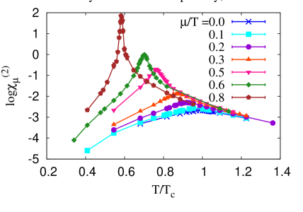
Figure 1: Chiral condensate and logarithmic scale of baryon number susceptibility on a $6^{3}\times 6$ lattice for various $\mu/T$ lines. The cross mark, square, circle, triangle, lower triangle, diamond, and pentagon denote $\mu/T=0.0,0.1,0.2,0.3,0.5,0.6$ and $0.8$, respectively.

2.2 Some remarks on the universality class

The staggered fermion has a remnant chiral symmetry in the chiral limit and has O(2) symmetry as long as the lattice spacing is coarse. We introduce the auxiliary fields to maintain the original symmetry, O(2). The auxiliary field action $S_{\mathrm{eff}}^{\mathrm{AF}}$ in Eq. (10) is invariant under the chiral transformation,

$$\begin{pmatrix}\sigma_{k}\\ \pi_{k}\end{pmatrix}\to\begin{pmatrix}\sigma_{k}^{\prime}\\ \pi_{k}^{\prime}\end{pmatrix}=\begin{pmatrix}\cos\Upsilon&-\sin\Upsilon\\ \sin\Upsilon&\cos\Upsilon\end{pmatrix}\begin{pmatrix}\sigma_{k}\\ \pi_{k}\end{pmatrix}\ ,$$ (13)

which corresponds to the transformation of the staggered fermion fields

$$\chi_{x}\to\chi_{x}^{\prime}=e^{i\varepsilon_{x}\Upsilon/2}\chi_{x}\ ,\quad{\bar{\chi}}_{x}\to{\bar{\chi}}_{x}^{\prime}=e^{i\varepsilon_{x}\Upsilon/2}{\bar{\chi}}_{x}\ .$$ (14)

In the framework of the MDP in the strong coupling limit, the critical exponent was studied and that values are consistent with O(2) MDP-CE . It should be noted that we need careful discussions about the difference in symmetry since the critical exponents are different in $\mathrm{O}(2)$, $\mathrm{O}(4)$, and Z(2). We will mention the relation between the O($N$) scaling function and critical behavior in Sec. 3.4.

3 Net-baryon number fluctuations in the strong coupling limit

3.1 Net-baryon number cumulants

In this section, we present results on the higher-order cumulant ratios of the net-baryon number. The $n$-th order cumulant of the net-baryon number in the grand canonical ensemble is given by

$$\chi_{\mu}^{(n)}=\frac{1}{VT^{3}}\frac{\partial^{n}\log Z}{\partial\hat{\mu}^{n}}\ ,\ \hat{\mu}=N_{c}\mu/T\ .$$ (15)

To discuss the effects of the phase transition on the net-baryon number fluctuations, it is convenient to take the ratio of a higher-order cumulant to the second order one CumuRatio ; CumuRatio-1 since the volume factor, $V$, in Eq. (15) cancels. We show the results of the following cumulant ratios, the normalized skewness and kurtosis,

$$S\sigma =\chi_{\mu}^{(3)}/\chi_{\mu}^{(2)}\ ,\quad\kappa\sigma^{2}=\chi_{\mu}^{(4)}/\chi_{\mu}^{(2)}.$$ (16)

The skewness $S$ and kurtosis $\kappa$ probe the asymmetry with respect to the mean and peakedness of the underlying probability distribution, respectively. The normalization by $\chi_{\mu}^{(2)}$ implies that one sets a reference, since $\kappa\sigma^{2}=1$ for the Skellam distribution which describes the distribution of the difference $n_{1}-n_{2}$, where $n_{1}$ and $n_{2}$ follow the Poisson distribution. Then it corresponds to the free hadron gas with Boltzmann approximation.

The detailed method for the calculation of the cumulants are summarized in Sec. A. As discussed in Sec. A, observables have an imaginary part due to the high $|\bf{k}|$ modes of $\pi_{{{\mathbb{k}},\tau}}$, so we take the real part of the observables and error bars in this article. The absolute mean value of maximum imaginary part for the normalized kurtosis and skewness are about 70 and 2 for $\mu/T=0.8$ and 0.5 and 0.04 for $\mu/T=0.2$, respectively, which are smaller than the peak heights and valley depth of the real part as seen in Figs. 3 and 4. It should be noted that the high temperature behavior of the cumulants would bare the artifacts of the present treatment. Figures 3 and 4 indicate that $S\sigma$ stays negative in the large chemical potential region and $\kappa\sigma^{2}$ can also take small negative values depending on $\mu/T$ at high $T$. For a free ideal baryon gas we expect $S\sigma\to 6\hat{\mu}/(3\hat{\mu}^{2}+\pi^{2})$ and $\kappa\sigma^{2}\to 6/(3\hat{\mu}^{2}+\pi^{2})$ at high temperature CumuRatio ; Stokic:2008jh ; Allton:2005gk . These differences at high temperature may be due to the truncation in the $1/d$ expansion. Spatial baryon hopping term is missing in the leading order in the $1/d$ expansion, then the fermion momentum integral generates only a volume factor. As a result, pressure is proportional to $T$ rather than $T^{4}$ in the Stefan-Boltzmann behavior at high temperature. Since we are interested in the transition region, where we expect that the long wave mesonic fluctuations dominate, we focus on the cumulant ratios around the phase boundary in the later discussion.

3.2 $T$ and $\mu$ dependence

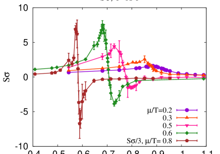
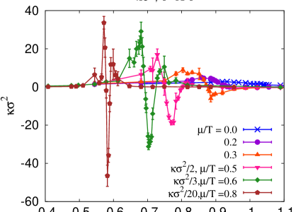
Figure 2: Normalized skewness (left panel) and kurtosis (right panel) on the various $\mu/T$ lines on a $6^{3}\times 6$ lattice The cross mark, circle, triangle, lower triangle, diamond, and pentagon indicate $\mu/T=0.0,\ 0.2,\ 0.3,\ 0.5,\ 0.6,$ and $0.8$ line, respectively. As for the skewness on the $\mu/T=0.8$ line, we rescale results by factor 3. For the kurtosis on the $\mu/T=0.5,0.6,0.8$ lines, we rescale results by factor 2, 3, 20, respectively.

In Fig. 2, we show the results of $S\sigma$ and $\kappa\sigma^{2}$ on a $6^{4}$ lattice at several $\mu/T$ as a function of $T/T_{c}$. One sees the strong dependence of these higher-order cumulants on both temperature and chemical potential. In the low chemical potential region, both $S\sigma$ and $\kappa\sigma^{2}$ are positive and have a broad peak.

As $\mu/T$ increases, characteristic structures emerge. $S\sigma$ increases with $T$, then exhibits a strong positive peak followed by sudden decrease to large negative value. Further increase of temperature leads to a constant small value. The negative region of the skewness, indicating the critical behavior CModel-3rd , starts to appear between $\mu/T=0.3$ and $\mu/T=0.5$. $\kappa\sigma^{2}$ shows similarly moderate increase with temperature and a sharp positive peak. Then it turns to be negative with a sharp valley but becomes positive again with a somewhat milder peak. Such an oscillatory behavior appears in $\mu/T>0.2$. Both cumulant ratios have one negative valley, and the skewness (kurtosis) has one (two) positive peak(s) at high chemical potential. Comparing with the phase boundary Ichihara:2014ova , one finds these behaviors appear around the phase boundary (see below). In the following subsections, we discuss the behaviors in more details by looking at lattice size dependence.

3.3 Lattice size dependence

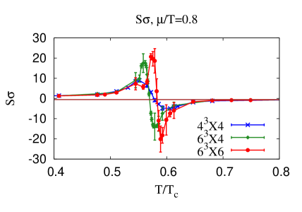
Figure 3: Normalized skewness on the $\mu/T=0.2$ (left panel) and $\mu/T=0.8$ (right panel) line on $4^{3}\times 4$ (the cross mark), $6^{3}\times 4$ (the diamond mark), and $6^{3}\times 6$ (the circle mark) lattices. A horizontal line around zero denotes the mean filed value at high temperature (see text). ($S\sigma\simeq-0.0220$ for $\mu/T=0.2$ and $S\sigma\simeq-0.5442$ for $\mu/T=0.8$.) We can find the negative region in the high chemical potential region.

In Figs. 3 and 4, we show the results of the normalized skewness $S\sigma$ and the normalized kurtosis $\kappa\sigma^{2}$, respectively, on the fixed $\mu/T$ lines, $\mu/T=0.2$ (left panel) and $\mu/T=0.8$ (right panel), on $4^{4},6^{3}\times 4$ and $6^{4}$ lattices. Horizontal lines show the mean field values at high temperature, where the chiral condensate vanishes. We will use these mean field values in Sec. 3.5 to remove the artifact as discussed in Sec. 3.1

Lattice size dependence of $S\sigma$ is moderate at low $\mu/T$ and prominent at large $\mu/T$. From Fig. 3, one sees that the qualitative structure of the temperature dependence of $S\sigma$ does not strongly depend on the lattice size. For $\mu/T=0.2$, the skewness is positive around the phase transition region and has a peak. While the peak height does not show statistically significant dependence on the lattice size, one finds the temperature dependence becomes slightly stronger in the largest one, $6^{4}$. The lattice size dependence becomes prominent at large chemical potential $\mu/T=0.8$. The skewness has one positive peak and one negative valley at $\mu/T=0.8$. The widths of the peak and the valley become narrower on a $6^{4}$ lattice.

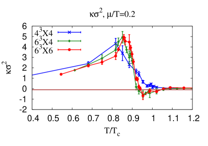
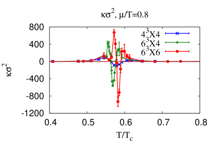
Figure 4: Normalized kurtosis on the $\mu/T=0.2$ (left panel) and $\mu/T=0.8$ (right panel) line on $4^{3}\times 4$ (the cross mark), $6^{3}\times 4$ (the diamond mark), and $6^{3}\times 6$ (the circle mark) lattices. The thin horizontal line around zero denotes the mean field value at high temperature (see text). ($\kappa\sigma^{2}\simeq-0.1033$ for $\mu/T=0.2$ and $\kappa\sigma^{2}\simeq-0.0251$ for $\mu/T=0.8$.)

Similar lattice size dependence is found for $\kappa\sigma^{2}$. In the low chemical potential region ($\mu/T=0.2$), the smallest lattice size $4^{4}$ does not exhibit the characteristic structure seen in larger lattice cases, but one sees a moderate decrease around $T/T_{c}\simeq 0.9$ following a peak at lower $T$. The broad negative valley appears on $6^{3}\times 4$ and $6^{4}$ lattices, implying that one should not take too small lattice size to see the influence of the critical fluctuations. We find that the oscillatory behavior with two positive peaks and one negative valley and its lattice size dependence becomes prominent for $\mu/T=0.8$. Again, as lattice size becomes larger, the peak height tends to be larger value and the width of the oscillatory region becomes narrower.

3.4 Relation to O($N$) scaling

The behavior of the higher-order net-baryon number cumulants around chiral phase transition are expected to be described by the property of the O($N$) scaling function O2-CE-alpha ; O4-CE-alpha ; SF-4 ; O2-O4-study ; SF-4-CM . According to Ref. SF-4-CM , the first divergent cumulant at $\mu=0$ in the thermodynamic limit is the sixth order one $\chi_{\mu}^{(6)}$ for $N=2$ and $4$. This result comes from the fact that the critical exponent of the specific heat $\alpha$ is negative in these cases, $\alpha\simeq-0.0147$ in O(2) O2-CE-alpha and $\alpha\simeq-0.21$ in O(4) O4-CE-alpha . For positive $\alpha$, the divergence appears at the fourth order cumulants while it has a cusp for $\alpha<0$ FRG-HM ; Morita_prob .

For a nonzero $\mu$, the first divergent cumulant is the third order one thus $S\sigma$ diverges in the thermodynamic limit for 3d O(2) and O(4) universality class. Once the singular part is smeared by the explicit breaking (nonzero current quark mass) or finite volume effects , the leading singular contribution is suppressed by the small multiplicative factor $-(2\kappa_{q})(\mu/T)^{n}$ where $\kappa_{q}$ denotes the curvature of the phase boundary near $\mu=0$ in the chiral limit SF-4-CM . Then, whether one sees the effects of critical fluctuations in the higher-order cumulants or not depends on the value of $\mu/T$ and magnitude of the regular part of the free energy density and its derivatives. For instance, $S\sigma$ positively (negatively) diverges in the thermodynamic limit when approached from below (above) the phase transition. The negative divergent contribution is replaced by a large negative value in the presence of the explicit breaking or finite volume effects. Then, the appearance of the negative $S\sigma$ depends on whether the singular part overcomes the regular part. Similar argument applies to $\kappa\sigma^{2}$, and the absence of the negative region in $\kappa\sigma^{2}$ in the smallest lattice (Fig. 4) is a consequence of the finite volume effects. Since $\kappa\sigma^{2}$ exhibits the oscillation around the phase transition along constant $\mu/T$ including the narrow negative region between the two positive peaks, one expects $\kappa\sigma^{2}$ positively diverges both from below and above the phase transition and negative region would disappear in the thermodynamic limit. The lattice size dependence of the negative $\kappa\sigma^{2}$ region meets this expectation. This is in contrast to the case of the finite quark mass. With finite quark mass, one finds the negative kurtosis region even in the thermodynamic limit as a remnant of the divergence in the chiral limit SF-4-CM ; FRG-HM .

3.5 Kurtosis in the QCD phase diagram in the strong coupling limit

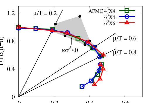
Figure 5: The negative kurtosis region in the QCD phase diagram in the chiral and strong coupling limit. The shaded area denotes the region where the $\kappa\sigma^{2}$ is both negative and smaller than the mean field value on a $6^{4}$ lattice (more detail explanations are in the text and footnote). The vertical axis is the temperature parametrized as $T=\gamma^{2}/N_{\tau}$ and the horizontal axis is the quark chemical potential. Both $T$ and $\mu$ are normalized by using $T_{c}$, the critical temperature at $\mu=0$ on a $6^{4}$ lattice. The phase boundaries on $4^{3}\times 4,6^{3}\times 4$, and $6^{3}\times 6$ lattices are determined by the peak position of the chiral susceptibility ($\chi_{\sigma}=\partial^{2}\log Z/\partial m_{0}^{2}/(L^{3}N_{\tau})$) for $\mu/T\leq 0.8$ and the effective potential analysis defined by $F_{\mathrm{eff}}=\left<S_{\mathrm{eff}}\right>/(N_{\tau}L^{3})$ for $\mu/T\geq 1.0$ Ichihara:2014ova . A gap is the expected boundary between the would-be 1st order and the would-be 2nd order transition.

In Fig. 5, we show the negative kurtosis region in the chiral limit $(m_{0}\rightarrow 0)$ on a $6^{4}$ lattice. We also show the phase boundary determined by the peak position of the chiral susceptibility ($\chi_{\sigma}=\partial^{2}\log Z/\partial m_{0}^{2}/(L^{3}N_{\tau})$) for $\mu/T\leq 0.8$ and by the cross point of the effective potential defined by $F_{\mathrm{eff}}=\left<S_{\mathrm{eff}}\right>/(N_{\tau}L^{3})$ for $\mu/T\geq 1.0$. The transition would be the second order for $\mu/T\leq 0.8$. While the numerical finite size scaling analysis cannot rule out crossover due to the statistics Ichihara:2014ova , we expect the second order transition from symmetry arguments PW84 . We guess that the tricritical point exists at $\mu/T>0.8$.

We here define the negative kurtosis region where $\kappa\sigma^{2}$ is smaller than the mean field results at high $T$, in order to reduce the artifact at high $T$ as discussed in Sec. 3.1. It should be noted that we do not take account of error bars to define the region here. The negative kurtosis region appears from about $\mu/T=0.2$, and the region is the largest at $\mu/T=0.3$ . By comparison, the kurtosis is positive at $\mu/T<0.2$. This might be due to the suppression of the singular contribution by the factor $(\mu/T)^{n}$ and the regular part dominates over the singular part SF-4-CM .

The negative $\kappa\sigma^{2}$ region almost coincides with the phase boundary. As discussed in Secs. 3.3 and 3.4, the region will shrink to the phase boundary and finally vanish in the thermodynamic limit. Although the dependence of the scaling function is different between the finite size effect and the symmetry breaking term, one could expect that the negative region also appears with finite mass in the strong coupling limit.

We conclude that we find the negative skewness or kurtosis region in the AFMC method in the chiral and strong coupling limit due to the finite volume effects as for the kurtosis, as a consequence of the critical fluctuations around the phase boundary incorporated through the AFMC method.

4 Summary

We have investigated the higher-order cumulant ratios of the net-baryon number, $S\sigma=\chi_{\mu}^{(3)}/\chi_{\mu}^{(2)}\ ,\kappa\sigma^{2}=\chi_{\mu}^{(4)}/\chi_{\mu}^{(2)}$, in the strong coupling $(g\rightarrow\infty)$ and the chiral limit ($m_{0}\rightarrow 0$) of QCD in the leading order of large dimensional expansions. Mesonic fluctuation effects are taken into account by making use of the auxiliary field Monte-Carlo (AFMC) method. We find the negative skewness and the kurtosis region around the boundary of the chiral phase transition. The skewness and kurtosis exhibit characteristic temperature dependences influenced by the critical fluctuations.

The skewness is found to be negative near the phase boundary for large $\mu/T$. The oscillatory behavior around the phase boundary seems to be consistent with the expectations from the finite volume effect such that the positive (negative) peak at lower (higher) temperature diverges in the thermodynamic limit SF-4-CM . Similarly, the kurtosis has one negative valley between two positive peaks for large $\mu/T$. With increasing lattice size, the negative valley is found to shrink, as anticipated for the finite volume effect. Thus, we expect two positive peaks diverge and the negative region disappears in the thermodynamic limit SF-4-CM .

One of the important next steps could be to study the effect of finite mass. This can be carried out by applying the AFMC method. Another important step is to see the finite size effects FSS ; ModelStudy-Volume-effect ; Vol-effect-study and determine the negative kurtosis area with or without bare quark mass. Whether one could have such region in lattice QCD is a mandatory question. As discussed above, it will depend on whether the smeared singular contribution by finite volume and/or explicit symmetry breaking term can overwhelm the regular contribution SF-4-CM ; ModelStudy-Volume-effect , which corresponds to hadron resonance gas in finite temperature QCD below the phase transition. Since our present formulation ignores the spatial baryon hopping, we would expect that the regular contribution might be smaller than the realistic case thus our results could serve as a lower limit for the value of chemical potential where $\kappa\sigma^{2}<0$.

Appendix A Higher order derivatives of the baryon chemical potential

In this appendix, we show the higher order derivatives with respect to dimensionless chemical potential $\hat{\mu}(=N_{c}\mu/T)$. In the following, the action $S$ and the partition function $Z$ are denoted as $S_{\mathrm{eff}}^{\mathrm{AF}}$ and ${\cal Z}_{\mathrm{AF}}$, respectively. Then, higher order derivatives are given as

$$\chi_{\mu}^{(1)} =\frac{1}{VT^{3}}\frac{\partial(\log Z)}{\partial\hat{\mu}}=\frac{1}{VT^{3}}\left[\frac{1}{Z}\int\mathcal{D}\Phi\left(-\frac{\partial S}{\partial\hat{\mu}}\right)e^{-S}\right]=\frac{1}{VT^{3}}\left<-\frac{\partial S}{\partial\hat{\mu}}\right>\ ,$$ (17)

$$\chi_{\mu}^{(2)} =\frac{1}{VT^{3}}\frac{\partial^{2}(\log Z)}{\partial\hat{\mu}^{2}}=\frac{1}{VT^{3}}\left[\left<\left(\frac{\partial S}{\partial\hat{\mu}}-\left<\frac{\partial S}{\partial\hat{\mu}}\right>\right)^{2}\right>-\left<\frac{\partial^{2}S}{\partial\hat{\mu}^{2}}\right>\right]\ ,$$ (18)

$$\chi_{\mu}^{(3)} =\frac{1}{VT^{3}}\frac{\partial^{3}(\log Z)}{\partial\hat{\mu}^{3}}$$

$$=\frac{1}{VT^{3}}\left[-\left<\left(\frac{\partial S}{\partial\hat{\mu}}-\left<\frac{\partial S}{\partial\hat{\mu}}\right>\right)^{3}\right>-\left<\frac{\partial^{3}S}{\partial\hat{\mu}^{3}}\right>+3\left<\left(\frac{\partial S}{\partial\hat{\mu}}-\left<\frac{\partial S}{\partial\hat{\mu}}\right>\right)\left(\frac{\partial^{2}S}{\partial\hat{\mu}^{2}}-\left<\frac{\partial^{2}S}{\partial\hat{\mu}^{2}}\right>\right)\right>\right]\ ,$$ (19)

$$\chi_{\mu}^{(4)} =\frac{1}{VT^{3}}\frac{\partial^{4}(\log Z)}{\partial\hat{\mu}^{4}}$$

$$=\frac{1}{VT^{3}}\left[\left<\left(\frac{\partial S}{\partial\hat{\mu}}-\left<\frac{\partial S}{\partial\hat{\mu}}\right>\right)^{4}\right>-3\left<\left(\frac{\partial S}{\partial\hat{\mu}}-\left<\frac{\partial S}{\partial\hat{\mu}}\right>\right)^{2}\right>^{2}+3\left<\left(\frac{\partial^{2}S}{\partial\hat{\mu}^{2}}-\left<\frac{\partial^{2}S}{\partial\hat{\mu}^{2}}\right>\right)^{2}\right>\right.$$

$$\left.-6\left<\left\{\left(\frac{\partial S}{\partial\hat{\mu}}\right)^{2}-\left<\left(\frac{\partial S}{\partial\hat{\mu}}\right)^{2}\right>\right\}\left(\frac{\partial^{2}S}{\partial\hat{\mu}^{2}}-\left<\frac{\partial^{2}S}{\partial\hat{\mu}^{2}}\right>\right)\right>\right.$$

$$\left.+4\left<\left(\frac{\partial S}{\partial\hat{\mu}}-\left<\frac{\partial S}{\partial\hat{\mu}}\right>\right)\left(\frac{\partial^{3}S}{\partial\hat{\mu}^{3}}-\left<\frac{\partial^{3}S}{\partial\hat{\mu}^{3}}\right>\right)\right>\right.$$

$$\left.+12\left<\frac{\partial S}{\partial\hat{\mu}}\right>\left<\left(\frac{\partial S}{\partial\hat{\mu}}-\left<\frac{\partial S}{\partial\hat{\mu}}\right>\right)\left(\frac{\partial^{2}S}{\partial\hat{\mu}^{2}}-\left<\frac{\partial^{2}S}{\partial\hat{\mu}^{2}}\right>\right)\right>-\left<\frac{\partial^{4}S}{\partial\hat{\mu}^{4}}\right>\right]\ ,$$ (20)

where $\hat{\mu}=N_{c}\mu/T$. The derivatives of the action with respect to $\hat{\mu}$ are given as

$$\frac{\partial S}{\partial\hat{\mu}} =-\sum_{\bm{x}}\frac{1}{R(\mathbb{x})}2\sinh\hat{\mu}\ ,$$ (21)

$$\frac{\partial^{2}S}{\partial\hat{\mu}^{2}} =\sum_{\bm{x}}\left[\frac{1}{R(\mathbb{x})^{2}}(2\sinh\hat{\mu})^{2}-\frac{1}{R(\mathbb{x})}2\cosh\hat{\mu}\right]\ ,$$ (22)

$$\frac{\partial^{3}S}{\partial\hat{\mu}^{3}} =\sum_{\bm{x}}\left[-\frac{2}{R(\mathbb{x})^{3}}(2\sinh\hat{\mu})^{3}+\frac{3}{R(\mathbb{x})^{2}}(2\sinh\hat{\mu})(2\cosh\hat{\mu})-\frac{1}{R(\mathbb{x})}2\sinh\hat{\mu}\right]\ ,$$ (23)

$$\frac{\partial^{4}S}{\partial\hat{\mu}^{4}} =\sum_{\bm{x}}\left[\frac{6}{R(\mathbb{x})^{4}}(2\sinh\hat{\mu})^{4}-\frac{12}{R(\mathbb{x})^{3}}(2\sinh\hat{\mu})^{2}2\cosh\hat{\mu}\right.$$

$$\left.\hskip 42.67912pt+\frac{3}{R(\mathbb{x})^{2}}(2\cosh\hat{\mu})^{2}+\frac{4}{R(\mathbb{x})^{2}}(2\sinh\hat{\mu})^{2}-\frac{1}{R(\mathbb{x})}2\cosh\hat{\mu}\right]\ ,$$ (24)

where $S=\sum_{\bm{k},\tau,f>0}\frac{L^{3}}{4N_{c}}f(\bm{k})\left[|\sigma_{\bm{k},\tau}|^{2}+|\pi_{\bm{k},\tau}|^{2}\right]-\sum_{\bm{x}}\log R(\mathbb{x})$ and $R(\mathbb{x})=X_{N}^{3}(\bm{x})-2X_{N}(\bm{x})+2\cosh\hat{\mu}$.

In this analysis, we have a complex phase coming from the fermion determinant, so the observables also take a complex value even if the observables are real in essence. Invoking the cancellation of the imaginary part in the case of higher statistics in principle, we can take the real part of the observables. We here use the jackknife method in order to evaluate the statistical errors JK . Since the observables have an imaginary part, we evaluate the error with complex phase and take the correlation between complex observables and the complex phase into account. Then, we take the real part of the obtained error bars.

When we evaluate the fourth derivative of $\log Z$ with respect to $\hat{\mu}$, $\chi_{\mu}^{(4)}$, (the function form is like $\left<\mathcal{O}\right>=\left<a\right>+\left<b\right>\left<c\right>+\left<d\right>^{2}$), we generate jackknife samples of each expectation value ($\left<a\right>_{\mathrm{bin}},\left<b\right>_{\mathrm{bin}},\left<c\right>_{\mathrm{bin}},\left<d\right>_{\mathrm{bin}}$). Then, we calculate the jackknife samples of the observable ($\left<\mathcal{O}\right>_{\mathrm{bin}}=\left<a\right>_{\mathrm{bin}}+\left<b\right>_{\mathrm{bin}}\left<c\right>_{\mathrm{bin}}+\left<d\right>_{\mathrm{bin}}^{2}$). Finally we calculate expectation value and error bars of the observable by using $\left<\mathcal{O}\right>_{\mathrm{bin}}$. When we calculate the cumulant ratios ($\kappa\sigma^{2}=\chi_{\mu}^{(4)}/\chi_{\mu}^{(2)},S\sigma=\chi_{\mu}^{(3)}/\chi_{\mu}^{(2)}$), we use the same technique as well.

References

- (1) M. A. Stephanov, K. Rajagopal, and E. V. Shuryak, Phys. Rev. Lett. 81, 4816 (1998); Phys. Rev. D 60, 114028 (1999).
- (2) M. Asakawa, U. W. Heinz and B. Müller, Phys. Rev. Lett. 85, 2072 (2000); S. Jeon and V. Koch, Phys. Rev. Lett. 85, 2076 (2000).
- (3) V. Koch, arXiv: 0810.2520.
- (4) M. M. Aggarwal et al. (STAR Collaboration), Phys. Rev. Lett. 105, 022302 (2010); L. Adamczyk, et al. (STAR Collaboration), Phys. Rev. Lett. 112, 032302 (2014).
- (5) Y. Hatta and M. A. Stephanov, Phys. Rev. Lett. 91, 102003 (2003).
- (6) M. Kitazawa and M. Asakawa, Phys. Rev. C 85, 021901 (2012).
- (7) L. Adamczyk et al. (STAR Collaboration), Phys. Rev. Lett. 113, 092301 (2014).
- (8) P. Braun-Munzinger, K. Redlich, and J. Stachel, in Quark-GluonPlasma 3, edited by R. C. Hwa and X. N. Wang (World Scientific, 2004) p. 491.
- (9) M. Kitazawa, M. Asakawa, and H. Ono, Phys. Lett. B 728, 386 (2014).
- (10) C. Sasaki, B. Friman, and K. Redlich, Phys. Rev. D 75, 074013 (2007).
- (11) K. Fukushima and T. Hatsuda, Rep. Prog. Phys. 74, 014001 (2011).
- (12) M. Asakawa and K. Yazaki, Nucl. Phys. A 504, 668 (1989).
- (13) Y. Hatta and T. Ikeda, Phys. Rev. D 67, 014028 (2003).
- (14) M. A. Stephanov, Phys. Rev. Lett. 102, 032301 (2009).
- (15) K. Morita, B. Friman, K. Redlich, and V. Skokov, Phys. Rev. C 88, 034903 (2013); K. Morita, V. Skokov, B. Friman, and K. Redlich, Eur. Phys. J. C 74, 2706 (2014); K. Morita, B. Friman, and K. Redlich, Phys. Lett. B 741, 178 (2015).
- (16) B. Friman, F. Karsch, K. Redlich, and V. Skokov, Eur. Phys. J. C 71, 1694 (2011).
- (17) M. A. Stephanov, Phys. Rev. Lett. 107, 052301 (2011).
- (18) R. D. Pisarski and F. Wilczek, Phys. Rev. D 29, 338 (1984).
- (19) S. Ejiri, F. Karsch, E. Laermann, C. Miao, S. Mukherjee, P. Petreczky, C. Schmidt, W. Soeldner, W. Unger, Phys. Rev. D 80, 094505 (2009); O. Kaczmarek, F. Karsch, E. Laermann, C. Miao, S. Mukherjee, P. Petreczky, C. Schmidt, W. Soeldner, and W. Unger, Phys. Rev. D 83, 014504 (2011); A. Bazavov, et. al., (HotQCD Collaboration), Phys. Rev. D 85, 054503 (2012).
- (20) Y. Aoki, G. Endrodi, Z. Fodor, S. D. Katz, and K. K. Szabo, Nature 443, 675 (2006); G. Endrodi, Z. Fodor, S. D. Katz, K. K. Szabo, JHEP 1104, 001 (2011).
- (21) H. Fujii and M. Ohtani, Phys. Rev. D 70, 014016 (2004).
- (22) A. Bazavov, H.-T. Ding, P. Hegde, O. Kaczmarek, F. Karsch, E. Laermann, Y. Maezawa and S. Mukherjee et al., Phys. Rev. Lett. 111, 082301 (2013) [arXiv:1304.7220 [hep-lat]]; R. Bellwied, S. Borsanyi, Z. Fodor, S. D. Katz and C. Ratti, Phys. Rev. Lett. 111, 202302 (2013) [arXiv:1305.6297 [hep-lat]]; A. Bazavov, H.-T. Ding, P. Hegde, O. Kaczmarek, F. Karsch, E. Laermann, Y. Maezawa and S. Mukherjee et al., Phys. Lett. B 737, 210 (2014) [arXiv:1404.4043 [hep-lat]]; A. Bazavov, H.-T. Ding, P. Hegde, O. Kaczmarek, F. Karsch, E. Laermann, Y. Maezawa and S. Mukherjee et al., Phys. Rev. Lett. 113, 072001 (2014) [arXiv:1404.6511 [hep-lat]]; S. Sharma [Bielefeld-BNL-CCNU Collaboration], Nucl. Phys. A 931, 1199 (2014) [arXiv:1408.2332 [hep-lat]]; H. T. Ding, Nucl. Phys. A 931, 52 (2014) [arXiv:1408.5236 [hep-lat]].
- (23) X. Y. Jin, Y. Kuramashi, Y. Nakamura, S. Takeda and A. Ukawa, Phys. Rev. D 91, 014508 (2015) [arXiv:1411.7461 [hep-lat]].
- (24) C. R. Allton, M. Doring, S. Ejiri, S. J. Hands, O. Kaczmarek, F. Karsch, E. Laermann and K. Redlich, Phys. Rev. D 71, 054508 (2005) [hep-lat/0501030];
- (25) C. Schmidt, Prog. Theor. Phys. Suppl. 186, 563 (2010) [arXiv:1007.5164 [hep-lat]]; R. V. Gavai and S. Gupta, Phys. Lett. B 696, 459 (2011) [arXiv:1001.3796 [hep-lat]]; A. Bazavov, H. T. Ding, P. Hegde, O. Kaczmarek, F. Karsch, E. Laermann, S. Mukherjee and P. Petreczky et al., Phys. Rev. Lett. 109, 192302 (2012) [arXiv:1208.1220 [hep-lat]].
- (26) S. Takeda, X. Y. Jin, Y. Kuramashi, Y. Nakamura and A. Ukawa, PoS LATTICE 2014, 196 (2014) [arXiv:1411.1148 [hep-lat]].
- (27) X. Y. Jin, Y. Kuramashi, Y. Nakamura, S. Takeda and A. Ukawa, Phys. Rev. D 88, 094508 (2013) [arXiv:1307.7205 [hep-lat]].
- (28) C. Gattringer and H. P. Schadler, Phys. Rev. D 91, 074511 (2015) [arXiv:1411.5133 [hep-lat]].
- (29) Z. Fodor, S. D. Katz, JHEP 0203, 014 (2002); JHEP 0404 , 050 (2004).
- (30) C. R. Allton, M. Döring, S. Ejiri, S. J. Hands, O. Kaczmarek, F. Karsch, E. Laermann, and K. Redlich, Phys. Rev. D 71, 054508 (2005); R. V. Gavai and S. Gupta, Phys. Rev. D 71, 114014 (2005) [hep-lat/0412035]; O. Kaczmarek, F. Karsch, E. Laermann, C. Miao, S. Mukherjee, P. Petreczky, C. Schmidt, W. Soeldner, and W. Unger, Phys. Rev. D 83, 014504 (2011).
- (31) H. Saito et al. [WHOT-QCD Collaboration], Phys. Rev. D 84, 054502 (2011) [Erratum-ibid. D 85, 079902 (2012)].
- (32) P. de Forcrand and O. Philipsen, Nucl. Phys. B 642, 290 (2002); JHEP 0701, 077 (2007); M. D’Elia and M. -P. Lombardo, Phys. Rev. D 67, 014505 (2003).
- (33) G. Aarts, E. Seiler and I. -O. Stamatescu, Phys. Rev. D 81, 054508 (2010); E. Seiler, D. Sexty, I. -O. Stamatescu, Phys. Lett. B 723, 213 (2013).
- (34) M. Cristoforetti, F. D. Renzo, and L. Scorzato [AuroraScience Collaboration], Phys. Rev. D 86, 074506 (2012); H. Fujii, D. Honda, M. Kato, Y. Kikukawa, S. Komatsu and T. Sano, JHEP 1310, 147 (2013).
- (35) K. Nagata and A. Nakamura, Phys. Rev. D 82, 094027 (2010).
- (36) A. Hasenfratz and D. Toussaint, Nucl. Phys. B 371, 539 (1992); S. Ejiri, Phys. Rev. D 78, 074507 (2008); A. Li, A. Alexandru and K. -F. Liu, Phys. Rev. D 84, 071503 (2011); K. Nagata, S. Motoki, Y. Nakagawa, A. Nakamura, and T. Saito (XQCD-J Collaboration), Prog. Theor. Exp. Phys. 2012, 01A103 (2012).
- (37) V. Skokov, B. Stokić, B. Friman, and K. Redlich, Phys. Rev. C 82, 015206 (2010); V. Skokov, B. Friman, and K. Redlich, Phys. Rev. C 83, 054904 (2011).
- (38) B. Stokić, B. Friman, and K. Redlich, Eur. Phys. J. C 67, 425 (2010).
- (39) K. Morita and K. Redlich, Prog. Theor. Exp. Phys. 2015, 043D03 (2015).
- (40) B. J. Schaefer and M. Wagner, Phys. Rev. D 85, 034027 (2012) [arXiv:1111.6871 [hep-ph]]; A. Bhattacharyya, S. K. Ghosh, A. Lahiri, S. Majumder, S. Raha and R. Ray, Phys. Rev. C 89, 064905 (2014) [arXiv:1212.6134 [hep-ph]].
- (41) M. Asakawa, S. Ejiri, and M. Kitazawa, Phys. Rev. Lett. 103, 262301 (2009),
- (42) B. -J. Schaefer and J. Wambach, Nucl. Phys. A 757, 479 (2005).
- (43) C. Wetterich, Phys. Lett. B 301, 90 (1993).
- (44) T. Ichihara, A. Ohnishi, and T. Z. Nakano, PTEP 2014 12, 123D02 (2014).
- (45) F. Karsch and K. H. Mutter, Nucl. Phys. B 313, 541 (1989).
- (46) G. Boyd, J. Fingberg, F. Karsch, L. Kärkkäinen, and B. Petersson, Nucl. Phys. B 376, 199 (1992).
- (47) P. de Forcrand and M. Fromm, Phys. Rev. Lett. 104, 112005 (2010) [arXiv:0907.1915 [hep-lat]]; W. Unger and P. de Forcrand, J. Phys. G 38, 124190 (2011) [arXiv:1107.1553 [hep-lat]].
- (48) M. Fromm, Ph.D. thesis, ETH-19297, Eidgenssische Technische Hochschule ETH Zrich, 2010.
- (49) P. de Forcrand, J. Langelage, O. Philipsen, and W. Unger, PoS LATTICE 2013, 142 (2013) [arXiv:1312.0589 [hep-lat]]; W. Unger, Acta Phys. Polon. Supp. 7 No. 1, 127 (2014).
- (50) N. Kawamoto and J. Smit, Nucl. Phys. B 192, 100 (1981); H. Kluberg-Stern, A. Morel, B. Petersson, Phys. Lett. B 114, 152 (1982); J. Hoek, N. Kawamoto, and J. Smit, Nucl. Phys. B 199, 495 (1982); P. H. Damgaard, N. Kawamoto and K. Shigemoto, Phys. Rev. Lett. 53, 2211 (1984); P. H. Damgaard, D. Hochberg, and N. Kawamoto, Phys. Lett. B 158, 239 (1985); P. H. Damgaard, N. Kawamoto, and K. Shigemoto, Nucl. Phys. B 264, 1 (1986).
- (51) H. Kluberg-Stern, A. Morel, B. Petersson, Nucl. Phys. B 215 [FS7], 527 (1983);
- (52) K. Fukushima, Prog. Theor. Phys. Suppl. 153, 204 (2004); Y. Nishida, Phys. Rev. D 69, 094501 (2004).
- (53) G. Faldt and B. Petersson, Nucl. Phys. B 265, 197 (1986).
- (54) N. Bilic, K. Demeterfi and B. Petersson, Nucl. Phys. B 377, 651 (1992).
- (55) N. Bilic, F. Karsch, and K. Redlich, Phys. Rev. D 45, 3228 (1992); N. Bilic and J. Cleymans, Phys. Lett. B 355, 266 (1995).
- (56) T. Jolicoeur, H. Kluberg-Stern, M. Lev, A. Morel, and B. Petersson, Nucl. Phys. B 235, 455 (1984).
- (57) I. Ichinose, Phys. Lett. B 135, 148 (1984); ibid. B 147, 449 (1984); I. Ichinose, Nucl. Phys. B 249, 715 (1985).
- (58) S. Aoki, Nucl. Phys. B 314, 79 (1989).
- (59) K. Miura, T. Z. Nakano and A. Ohnishi, Prog. Theor. Phys. 122, 1045 (2009); K. Miura, T. Z. Nakano, A. Ohnishi and N. Kawamoto, Phys. Rev. D 80, 074034 (2009).
- (60) T. Z. Nakano, K. Miura and A. Ohnishi, Prog. Theor. Phys. 123, 825 (2010).
- (61) T. Z. Nakano, K. Miura, and A. Ohnishi, Phys. Rev. D 83 (2011) 016014.
- (62) K. Fukushima, Phys. Lett. B 591, 277 (2004) [hep-ph/0310121]; C. Ratti, M. A. Thaler and W. Weise, Phys. Rev. D 73, 014019 (2006) [hep-ph/0506234]. K. Morita, V. Skokov, B. Friman and K. Redlich, Phys. Rev. D 84, 076009 (2011) [arXiv:1107.2273 [hep-ph]].
- (63) F. Karsch, S. Ejiri and K. Redlich, Nucl. Phys. A 774, 619 (2006) [hep-ph/0510126]; S. Ejiri, F. Karsch, and K. Redlich, Phys. Lett. B 633, 275 (2006).
- (64) F. Karsch and K. Redlich, Phys. Lett. B 695, 136 (2011).
- (65) B. Stokic, B. Friman and K. Redlich, Phys. Lett. B 673, 192 (2009) [arXiv:0809.3129 [hep-ph]].
- (66) M. Campostrini, M. Hasenbusch, A. Pelissetto, P. Rossi and E. Vicari, Phys. Rev. B 63, 214503 (2001) [cond-mat/0010360].
- (67) J. Engels and F. Karsch, Phys. Rev. D 85, 094506 (2012).
- (68) J. Engels and F. Karsch, Phys. Rev. D 90, 014501 (2014).
- (69) J. Engels and T. Mendes, Nucl. Phys. B 572, 289 (2000); J. Engels, S. Holtmann, T. Mendes and T. Schulze, Phys. Lett. B 492, 219 (2000); J. Engels, S. Holtmann, T. Mendes and T. Schulze, Phys. Lett. B 514, 299 (2001); A. Cucchieri, J. Engels, S. Holtmann, T. Mendes and T. Schulze, J. Phys. A 35, 6517 (2002);
- (70) R. A. Tripolt, J. Braun, B. Klein and B. J. Schaefer, Phys. Rev. D 90, 054012 (2014); Phys. Rev. C 91, 041901 (2015); A. Bhattacharyya, R. Ray and S. Sur, Phys. Rev. D 91, 051501 (2015).
- (71) X. Pan, L. Chen, X. S. Chen and Y. Wu, Nucl. Phys. A 913, 206 (2013).
- (72) B. Friman, Nucl. Phys. A 928, 198 (2014) [arXiv:1404.7471 [nucl-th]].
- (73) J. Braun and B. Klein, Eur. Phys. J. C 63, 443 (2009) [arXiv:0810.0857 [hep-ph]]; J. Braun, B. Klein and P. Piasecki, Eur. Phys. J. C 71, 1576 (2011) [arXiv:1008.2155 [hep-ph]]; J. Braun, B. Klein and B. J. Schaefer, Phys. Lett. B 713, 216 (2012) [arXiv:1110.0849 [hep-ph]]; P. Springer and B. Klein, arXiv:1506.00909 [hep-ph].
- (74) For example, I. Montvay and G. Munster, Quantum Fields on a Lattice (Cambridge University Press, Cambridge, 1994)