Non-parametric estimation of Fisher information from real data

Abstract

The Fisher Information matrix is a widely used measure for applications ranging from statistical inference, information geometry, experiment design, to the study of criticality in biological systems. Yet there is no commonly accepted non-parametric algorithm to estimate it from real data. In this rapid communication we show how to accurately estimate the Fisher information in a non-parametric way. We also develop a numerical procedure to minimize the errors by choosing the interval of the finite difference scheme necessary to compute the derivatives in the definition of the Fisher information. Our method uses the recently published “Density Estimation using Field Theory” algorithm to compute the probability density functions for continuous densities. We use the Fisher information of the normal distribution to validate our method and as an example we compute the temperature component of the Fisher Information Matrix in the two dimensional Ising model and show that it obeys the expected relation to the heat capacity and therefore peaks at the phase transition at the correct critical temperature.

Consider a probabilistic description of a system as a probability density function (PDF) $p(x;\theta)$. The observables of the system are collected as parts of the vector $x$ and the PDF will typically depend on a vector of continuous parameters $\theta$. It is interesting how the system responds to parameter changes, e.g. at phase transitions or system dynamics near bifurcations. A measure of the sensitivity of the PDF to the parameters is the Fisher Information Matrix (FIM) Cover and Thomas (2006). It is a symmetric matrix labeled by the parameters of the PDF. If a small parameter change causes a large change in the PDF, the corresponding entry in the FIM will be large. Much literature discusses the different uses of the FIM, its interpretation as a Riemmanian metric on the statistical manifold Amari and Nagaoka (2000) and its relation to theories of phase transitions Ruppeiner (1979); Ruppeiner and Davis (1990); Ruppeiner (1995); Ruppeiner et al. (2012); Ingarden et al. (1982); Janyszek and Mrugala (1989); Janyszek (1990); Brody and Rivier (1995); Brody and Hook (2009); Kumar et al. (2012) and complex systems Obata et al. (1992, 1997); Mayer et al. (2006); Frank (2009); Prokopenko et al. (2011); Wang et al. (2011); Hidalgo et al. (2014).

Since the FIM is directly computed from the PDF, its accurate estimation depends on the general density estimation problem Silverman (1986). Density estimation aims to obtain the best estimate $Q_{\mathrm{est}}$ of a distribution $Q_{\mathrm{true}}$ given $N$ independently drawn samples. We distinguish between parametric and non-parametric estimation. Parametric estimates constrain $Q_{\mathrm{est}}$ to depend on a few parameters that are estimated from the data Walter and Pronzato (1997). By the Cramér-Rao inequality Cover and Thomas (2006) the inverse of the Fisher information (FI) is a lower-bound on the variance of the estimated parameters. FI is therefore often computed in the parametric setting. In these cases the FI is computed analytically from the assumed function.

When we do not assume a specific form for the PDF, we estimate the density non-parametrically. Thus, the data determines the shape of the distribution. Areas with higher probability density will contain more data points than areas with lower probability. The main problem of non-parametric methods is how to balance the goodness of fit to the data and the smoothness of the estimated curve Silverman (1986). For example, kernel density estimators (KDEs) are a sum over kernel functions with width $h$, positioned at each data point. i.e. $Q_{\mathrm{est}}(x)=(hN)^{-1}\sum\limits_{i=1}^{N}K[(x-x_{i})/h]$ where $x_{i}$ is a data point and $K$ is a kernel function. The bandwidth $h$ controls the smoothness of the estimate. In the limit $h\rightarrow 0$ the estimate is a sum of delta functions at each data point; in the $h\rightarrow\infty$ it is uniform. Choosing the correct bandwidth is therefore important. Taken too large, the estimate will hide crucial features. Too small a bandwidth causes spurious peaks in the estimate, especially for long-tailed distributions Silverman (1986). Important to this study, the amount of smoothing directly affects the value of the FI. This can be seen from its definition:

$$g_{\mu\nu}(\theta)=\langle(\partial_{\mu}\ln p)(\partial_{\nu}\ln p)\rangle\,,$$ (1)

which depends on the derivatives of the PDF. Here $\partial_{\mu}\equiv\partial/\partial\theta^{\mu}$, $p$ is a PDF and the average is with respect to $p$. If, e.g., the estimated PDF $Q_{\mathrm{est}}$ is smoother than the true PDF $Q_{\mathrm{true}}$, the estimate for the FI will be smaller than the true FI.

One elegant approach that derives the smoothness from the data itself was proposed in Bialek et al. (1996). The authors used field theory to formulate the notion of a smoothness scale as an ultraviolet cutoff, treating the smoothness length scale $\ell$ as a parameter in a Bayesian inference procedure. They showed that, in the large $N$ limit, the data selects an appropriate length scale. Recently, this method was developed into a fast and accurate algorithm called DEFT (Density Estimation using Field Theory) Kinney (2014). The algorithm was implemented in one and two dimensions, since it suffers from the “curse of dimensionality” Kinney (2014).

Previous work on the nonparametric estimation of FI primarily dealt with PDFs with location-like parameters, i.e. $p(x;\theta)=p(x-\theta)$. There Huber Huber (1974) found a unique interpolation of the cumulative distribution function that maximizes the FI. Kostal and Pokora Kostal and Pokora (2012) adapted the maximized penalized likelihood method of Goodd and Gaskins Goodd and Gaskins (1971) to compute the FI. Kostal and Pokora rejected the use of KDE for the direct computation of the FI because no appropriate bandwidth parameter to control of the $p^{\prime}/p$ term in (1) is known Kostal and Pokora (2012). In this work we estimate PDFs from samples drawn from the normal distribution at different parameter values using both DEFT and KDE with a Gaussian kernel, and compare the FI results to the analytic solution. We obtain accurate results using DEFT, which are an improvement over using KDE. We also use DEFT to compute the FI in the two dimensional Ising model showing the computation is accurate also at the phase transition.

To proceed we replace the derivatives in Eq. (1) with centered finite-difference derivatives:

$$g_{\mu\nu}(\theta) \approx\int\frac{p(x;\theta+\Delta\theta^{\mu})-p(x;\theta-\Delta\theta^{\mu})}{2\Delta\theta^{\mu}}$$ (2a)

$$\times\frac{p(x;\theta+\Delta\theta^{\nu})-p(x;\theta-\Delta\theta^{\nu})}{2\Delta\theta^{\nu}}\frac{dx}{p(x;\theta)}$$

$$\approx\int\frac{\ln p(x;\theta+\Delta\theta^{\mu})-\ln p(x;\theta-\Delta\theta^{\mu})}{2\Delta\theta^{\mu}}$$ (2b)

$$\times\frac{\ln p(x;\theta+\Delta\theta^{\nu})-\ln p(x;\theta-\Delta\theta^{\nu})}{2\Delta\theta^{\nu}}p(x;\theta)dx\,.$$

Here $\Delta\theta^{\mu}$ indicates a change in the value of only one parameter $\theta^{\mu}$ keeping all other parameters fixed, i.e., $\theta+\Delta\theta^{\mu}\equiv(\theta^{1},\ldots,\theta^{\mu}+\Delta\theta^{\mu},\ldots,\theta^{d})$. The error introduced by this replacement is proportional to $O(\Delta\theta^{2}/6)$ (for each derivative) as can be verified by Taylor expansion. Higher order finite-difference schemes can be used but not, in our experience, a lower order one-sided derivative because the estimate does not converge to the true value (data not shown).

This introduces a new free parameter: the size of the difference $\Delta\theta^{\mu}$. The value of $\Delta\theta^{\mu}$ strongly influences the accuracy of the computation. Two sources of error determine the optimal $\Delta\theta^{\mu}$: the aforementioned numerical derivative error and the finite sample size $N$. The first error, which scales like $O[(\Delta\theta^{\mu})^{2}]$, decreases with decreasing $\Delta\theta$. The second source, however, decreases with increasing $\Delta\theta^{\mu}$. This happens because an estimate from a finite number of samples is always under-determined. Any estimate is one curve from a group of curves that are close, but not equal, to the true density. The larger the number of samples, the smaller the size of the group. If $\Delta\theta^{\mu}$ is too small, the groups of the densities in the numerical derivatives will overlap and the difference $p(x;\theta+\Delta\theta^{\mu})-p(x;\theta-\Delta\theta^{\mu})$ will be ill-defined. This leads to one of our main results: since $\Delta\theta^{\mu}$ cannot be too small or too large, there is an optimal value with minimal error between the two extremes.

To estimate the curve group size and avoid overlaps, we use large deviations theory. According to Sanov’s theorem Sanov (1957) the appropriate distance measure is the Kullback-Leibler (KL) divergence:

$$\mathcal{D}_{KL}[Q||P]\equiv\int\limits_{x\in\mathcal{X}}Q(x)\ln\frac{Q(x)}{P(x)}dx$$ (3)

which is defined for two densities $P(x)$ and $Q(x)$ where the support of $P$ and $Q$ overlap. The probability that a set of $N$ samples independently drawn from $P$ appears to be drawn from $Q$ is proportional to:

$$\exp\left(-N\mathcal{D}_{KL}\left[Q||P\right]\right).$$ (4)

In the limit of infinite sample size this tends to zero. For finite $N$ the set of distributions whose KL-divergence with $P$ is small enough such that this probability is finite forms the curve group. This can be interpreted as a hypersphere in parameter space centered at $\theta$ with an $N$ and $\theta$ dependent radius. To minimize error, the radius at $\theta$ and $\theta+\Delta\theta^{\mu}$ should be small compared to $\Delta\theta^{\mu}$. The ideal case is drawn schematically in Fig. 1a with well separated densities and in Fig. 1b where $\Delta\theta^{\mu}$ is too small.

(a) Well separated densities.

(b) Overlapping densities.

Figure 1: Schematic drawing in one dimension with points of estimation $\theta$ and $\theta+\Delta\theta$. The gray area is the hypersphere. $\varepsilon$ is the radius of the hypersphere in units of $\Delta\theta$.

To compute hypersphere radius we take $P=p(x;\theta)$ and $Q=p(x;\theta+\varepsilon\Delta\theta^{\mu})$ in Eq. (4). We thus seek the density $Q$ at the edge of the hypersphere and parametrize it with $\varepsilon$, the hypersphere radius in units of $\Delta\theta^{\mu}$. The KL-divergence of two neighbouring distributions is approximately:

$$\mathcal{D}_{KL}[P(\theta)||P(\theta+\varepsilon\Delta\theta^{\mu})]\approx\frac{\varepsilon^{2}}{2}g_{\mu\nu}(\theta)\Delta\theta^{\mu}\Delta\theta^{\nu}=O(\Delta\theta^{2})$$ (5)

where we use the Einstein summation convention for repeated indices . Inserting Eq. (5) into Eq. (4) we get

$$\exp\left[-\frac{N\varepsilon^{2}}{2}g_{\mu\nu}(\theta)\Delta\theta^{\mu}\Delta\theta^{\nu}\right].$$ (6)

We define the boundary of the hypersphere as the point where the probability is equal to $e^{-1}$. Equating Eq. (6) with $e^{-1}$, we obtain the radius $\varepsilon$:

$$\varepsilon^{2}=\frac{2}{Ng_{\mu\nu}(\theta)\Delta\theta^{\mu}\Delta\theta^{\nu}}\,.$$ (7)

The radius depends on the number of samples $N$, $\theta$, and $\Delta\theta^{\mu}$. At a given $N$ and $\theta$, increasing $\Delta\theta^{\mu}$ will decrease the radius and thus increase accuracy.

As an analytically solvable example, we take the univariate normal distribution $\mathcal{N}(\mu,\sigma)$. Its FI is

$$g_{\mu\mu}=\frac{1}{\sigma^{2}};\quad g_{\sigma\sigma}=\frac{2}{\sigma^{2}};\quad g_{\mu\sigma}=g_{\sigma\mu}=0\,.$$ (8)

We focus on the FI of $\sigma$, which is not a location parameter. Inserting this to Eq. (7) yields

$$\Delta\sigma=\sqrt{\frac{2}{\varepsilon^{2}Ng_{\sigma\sigma}}}=\frac{\sigma}{\varepsilon\sqrt{N}}\,,$$ (9)

with $\Delta\sigma\equiv\Delta\theta^{\sigma}$. This guides the choice of $\Delta\sigma$ for a given $N$, $\sigma$, and desired radius $\varepsilon$. We can get the same result using the Cramér-Rao inequality. The minimal variance of an unbiased estimator for $\sigma$ is $1/g_{\sigma\sigma}$. Given $N$ samples this equals $\sigma^{2}/2N$. Demand that the variance of $\sigma$ is equal to $\frac{1}{2}{(\varepsilon\Delta\sigma)}^{2}$ (the factor $\frac{1}{2}$ ensures a consistent definition of $\varepsilon$). This variance is equivalent to a hypersphere radius of $\varepsilon\Delta\sigma$. We then have $\sigma^{2}/2N={(\varepsilon\Delta\sigma)}^{2}/2$. Solving for $\Delta\sigma$ yields Eq. (9).

For real data the FI is unknown and can be estimated iteratively. First compute the FI with $\Delta\theta^{\mu}$ that ensure a good approximation of the numerical derivatives. Then use the FI to compute $\varepsilon$. If it is too large ($\varepsilon\approx 0.1$ seems to be reasonable), increase $\Delta\theta^{\mu}$ or $N$.

We demonstrate our main results by computing $g_{\sigma\sigma}$ from independently drawn normally distributed samples. We first compare DEFT (with number of grid points $G=100$, smoothness parameter $\alpha=3$ and a bounding box twice the interval between the smallest and largest sample Kinney (2014)) and KDE (using Scott’s rule for the bandwidth). We used both with the same samples and computed the FI from Eq. (2). In the top plot of Fig. 2 the FI estimate is shown. The black curve is the analytic value, the green dots and blue $\times$’s are the median estimate after $100$ repetitions (error bars are $5$ and $95$ percentiles) for DEFT and KDE respectively. We used $N=10^{4}$ for each density estimate. We used $\varepsilon=0.05$ since this yields the best results.

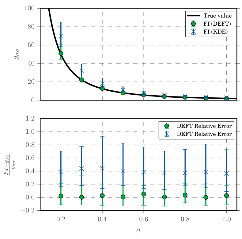
Figure 2: (Color online) A comparison between Gaussian KDE and DEFT for density estimation. Top figure shows median FI estimates using both methods. Error bars represent $5$ and $95$ percentiles. Bottom figure shows the relative errors. The values were computed with $N=10^{4}$, $\varepsilon=0.05$, and $100$ repetitions at each $\sigma$. The same samples were used by both methods.

Both methods seem to follow the analytic curve, however from the relative errors it is clear that KDE consistently overestimates the FI by about $40\%$ and the distance between $5$ and $95$ percentile is about $100\%$ of the original value. DEFT has zero bias and a spread of $30\%-40\%$. We conclude that DEFT provides an improvement over KDE both in the estimated value and in the error margins. In the above computations we used Eq. (2a) for computation with DEFT and Eq. (2b) for KDE, because KDE was extremely unstable when computed using Eq. (2a) while DEFT performed slightly better with Eq. (2a).

In the following we use DEFT exclusively for the density estimation. To see how the error depends on $\varepsilon$ we vary it at a fixed $N=2\times 10^{4}$ and plot the relative error. We computed the FI for $\sigma=0.5,1,2,5,10$. Each computation was repeated $100$ times at different $\varepsilon$ and the median and $5$ and $95$ percentiles of the relative error ($[g_{\sigma\sigma}-FI]/g_{\sigma\sigma}$, where $FI$ is the estimated FI) were computed. All curves have the same functional dependence on $\varepsilon$ and, as we predicted, there is an optimal value for $\Delta\sigma$, at $\varepsilon\approx 0.05$. Thus the errors depend on $\sigma$ through the combination in Eq. (7), as shown in Fig. 3. All the curves have a minimum in the range of $\varepsilon\in[0.04,0.1]$. At small $\varepsilon$ they grow due to errors in the numerical derivative ($\Delta\sigma$ too large). At large $\varepsilon$ they grow due to overlapping densities. The spread (the $90\%$ inter-percentile range) is minimal at $\varepsilon=0.05$ as well. The shaded regions in the plot represent the inter-percentile range of the various $\sigma$ curves.

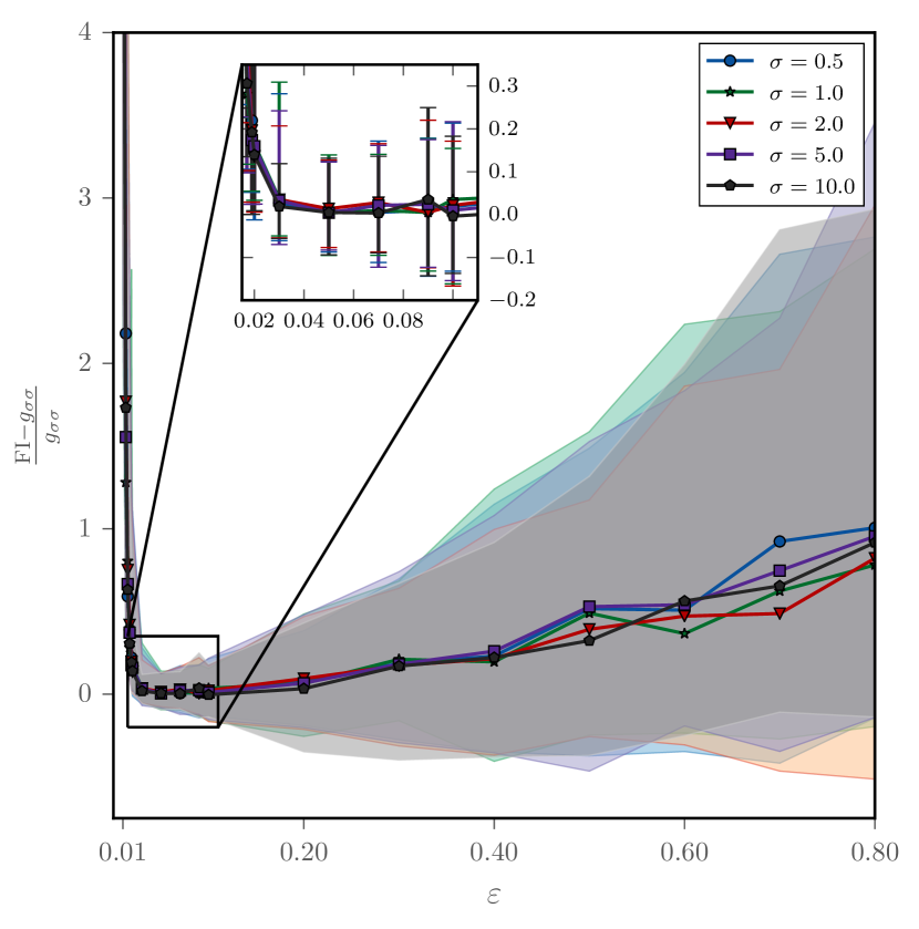
Figure 3: (Color online) The median relative error as a function of $\varepsilon$ for different values of $\sigma$. FI stands for the computed value and $g_{\sigma\sigma}$ the analytic value. The shaded areas and error bars in the inset indicate the $5$ and $95$ percentiles computed over 100 repetitions of the computation with $N=2\times 10^{4}$.

To verify the $N$ and $\varepsilon$ dependence of the errors we varied both and computed $g_{\sigma\sigma}$. The result is presented as a heat map in Fig. 4. The color represents the absolute-value relative estimation error in logarithmic scale. The dashed line indicates the $\varepsilon=0.1$ line which represents the highest value of $\varepsilon$ where good results are still obtained. The dash-dotted line represents the $\Delta\sigma=0.35$ line. All computations were done with $\sigma=1.0$ and $100$ repetitions. The errors due to small $\Delta\sigma$ seem to follow the $\varepsilon=0.1$ curve, showing again the dependence of this type of error on $\varepsilon$. Above $\Delta\sigma=0.35$ we see increasing errors due to the large value of $\Delta\sigma$. The best area for the estimation is between the two lines.

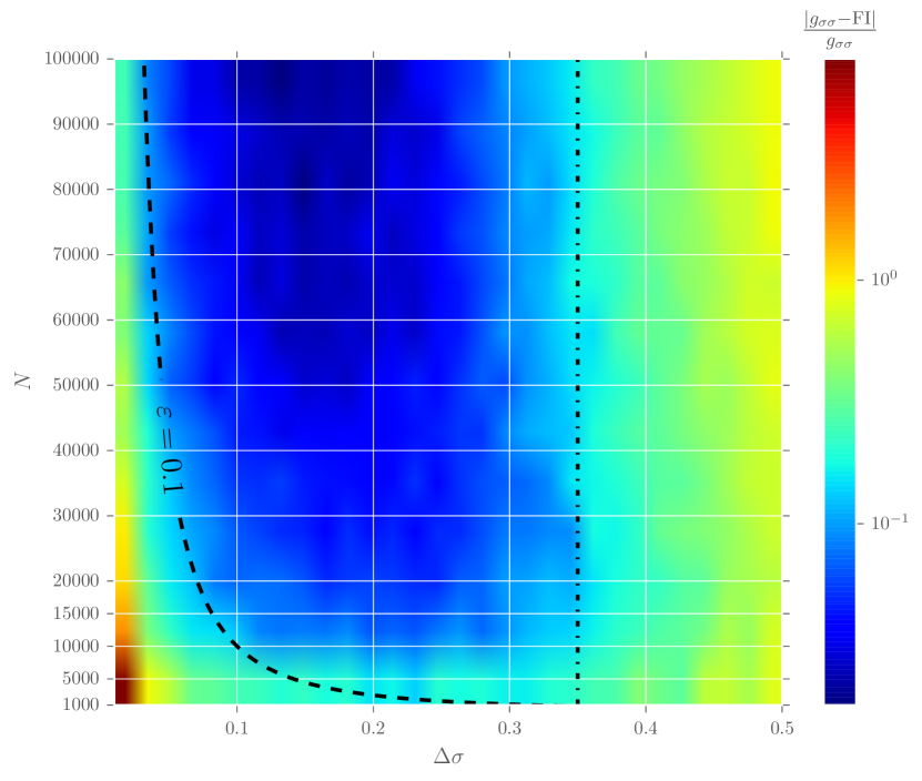
Figure 4: (Color online) Relative error in the computation of the FI for $\sigma=1.0$ as a function of both $\Delta\sigma$ and $N$. Computed using DEFT with $100$ repetitions per point. Dashed line represents the $\varepsilon=0.1$ line and the dash-dotted line is the $\Delta\sigma=0.35$ line. Unlike the previous plots, here we compute the absolute value relative error to avoid problems with the logarithmic color-bar scale.

One of the applications of the computation of FI from samples is in detecting phase transitions Prokopenko et al. (2011). As a further validation we took the two dimensional Ising model, which is the prototypical model of a continuous phase transition. It is a model of binary spins $s_{i}$ on a square lattice with nearest-neighbors interaction. Its Hamiltonian is

$$\mathcal{H}=-\sum\limits_{\langle i,j\rangle}J_{ij}s_{i}s_{j}-h\sum\limits_{i}s_{i}\,,$$ (10)

where $\langle i,j\rangle$ indicates the sum is on nearest neighbors, $s_{i}=\pm 1$ is the value of a spin at site $i$, $J_{ij}$ is the interaction energy, and $h$ is an external applied magnetic field. In more than one dimensions there is a critical order-disorder phase transition at a finite temperature. Onsager solved the model exactly in two dimensions in the thermodynamic limit (infinite number of spins) and at zero applied external field Onsager (1944). The critical temperature in the isotropic case ($J_{ij}\equiv J$) is

$$T_{c}=\frac{2J}{\ln(1+\sqrt{2})}\approx 2.269J\,.$$ (11)

For simplicity we set $J\equiv 1$ and Boltzmann’s constant $k_{B}\equiv 1$.

Prokopenko et. al. Prokopenko et al. (2011) computed both the $TT$ and $hh$ components of the FI (computed for the Gibbs distribution with $\theta^{1}=h$ and $\theta^{2}=T$) in terms of the susceptibility $\chi_{T}$ and the specific heat $C_{h}$ and showed that:

$$g_{TT}=\frac{C_{h}}{T^{2}}\,;\quad g_{hh}=\frac{\chi_{T}}{T}\,.$$ (12)

We therefore expect both to diverge as the system approaches the critical temperature. In a finite system this means that the FI peaks at the critical temperature.

To validate this result we simulate the Ising model and compute the FI. We used the Metropolis-Hastings Monte Carlo algorithm to obtain samples of the configuration energy with the Gibbs distribution (at zero external field):

$$p(S;T)=\frac{1}{Z(T)}\exp\left[-\beta\mathcal{H}(S,T,h=0)\right].$$ (13)

Here $\beta=1/T$ is the inverse temperature, $S={\{s_{i}\}}_{i=1,\ldots,L^{2}}$ is a configuration of the spins on a $L\times L$ square lattice, and $Z$ is the partition function. We then estimate the $TT$ component of the FI using Eq. (2) with densities estimated from the sampled energies. We also computed the specific heat:

$$C_{h}(T)=\frac{1}{L^{2}T^{2}}\left(\langle E^{2}\rangle-\langle E\rangle^{2}\right)$$ (14)

where $L^{2}$ is the total number of spins, $E$ is the energy of the configuration, and the average is performed over different configurations at the same temperature.

We plot the result of both the FI and the specific heat $C_{h}$ computation in Fig. 5. The simulation was run on a $25\times 25$ lattice of spins with periodic boundary conditions in the temperature range $[0.5,4.0]$ which we divided into $200$ segments, leading to parameter difference of $dT\simeq 0.17$. We repeated the simulation $5$ times and compute the median and $5$ and $95$ percentiles. We used a warm-up period of $5\times 10^{6}$ time steps and took $N=15,000$ samples of the configuration energy. We used DEFT (with $G=200$, $\alpha=3$ and a bounding box of $[-4,1]$) for the density estimation. Because the FI depends on $T$, $\varepsilon$ was not constant. Its median was $\varepsilon=0.12\begin{subarray}{c}+0.12\\ -0.07\end{subarray}$ for the values of $\varepsilon$ which were not infinite. To verify that Eq. (12) holds, we plot the ratio of the two sides of the equation. This is presented in the inset in Fig. 5.

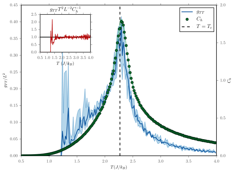
Figure 5: (Color online) Blue continuous curve is the $TT$ component of the FIM and the green dots are the heat capacity in the $2D$ Ising model on a $25\times 25$ grid. Shaded blue and green regions indicates the $5$ and $95$ percentiles computed from $5$ simulations. Inset shows the ratio of FI to heat capacity ($g_{TT}T^{2}C_{v}^{-1}L^{-2}$) which according to Eq. (12) is equal to $1$.

There are several technical points we would like to mention about the implementation of the method. First, we performed the same computation with a smaller grid spacing ($dT=0.007$). This led to a much worse signal-to-noise ratio because the very close densities caused large peaks to occur, especially in the low temperature range. Second, it is important to find the most suitable parameters for DEFT. If the bounding box is too small, or the number of grid points too small or too large, the estimated density will have multiple peaks which are not apparent in the data. Thus we recommend plotting the result of DEFT together with a histogram for several data points to make sure the convergence is good. Third, in the computation of Eq. (2a) the term $1/p$ may contribute large values at very small $p$. Equivalently with Eq. (2b), when $p(x|\theta\pm\Delta\theta)$ are small, their logarithm will again be large. This requires the introduction of a numerical cutoff. It is common practice to set the contribution of a term where $p(x)=0$ to zero Wang et al. (2011). We thus introduced a cutoff such that if any of the estimates at a particular point is less than the cutoff, the contribution of this point to the integral will be zero. We investigated the effect of this cutoff for a range of values between $10^{-20}$ and $10^{-2}$. The value of the cutoff had very little effect. In the Ising model, the only effect was to change the size of the low temperature region where the FI is exactly zero (the lower the cutoff, the smaller the region was). In producing Fig. 5 we used a value of $10^{-10}$. Lastly we would like to mention that the plots in Fig. 5 were obtained by the use of Eq. (2b).

As is clear by the remarks above, care should be taken when using this method to compute the FI. One should first make sure a good convergence of DEFT is achieved, by adjusting $G$, $\alpha$ and the bounding box. Then make sure to select the correct parameter difference $\Delta\theta$, a decision that can be aided by the estimation of the $\varepsilon$ parameter. And if necessary, use a cutoff for very low values of the probability density. Since we rely on DEFT to perform the density estimation, the procedure is limited by the limitations of DEFT. It is especially important to note that so far DEFT has been implemented in $1$ and $2$ dimensions. Higher dimensions suffer from the “curse of dimensionality” since they require exponentially many grid points to evaluate the density.