Quadratic forms of the empirical processes for the two sample problem for functional data

Abstract

The use of quadratic forms of the empirical process for the two-sample problem in the context of functional data is considered. The convergence of the family of statistics proposed to a Gaussian limit is established under metric entropy conditions for smooth functional data. The applicability of the proposed methodology is evaluated in examples.

Keywords: Functional data; two-sample problem; empirical processes; random sea waves.

1 Introduction

Functional data analysis has had a very important growth in the last 20 years, and has found applications in many different areas, especially since the first edition of the book by Ramsay and Silverman in 1997. More recent contributions to the field can be found in Bosq (2000), Ramsay and Silverman (2002, 2005), Ferraty and Vieu (2006), Ferraty (2011) and Horváth and Kokoszka (2012), where examples of diverse applications can also be found.

In the analysis of functional data a frequent problem is that of deciding if two samples of functions come from the same population. Let $X_{1}(t),\cdots,X_{m}(t)$ be an i.i.d. sample of real valued curves defined on some interval $J$. Denote by $\mathcal{L}(X)$ the probability law producing these curves. Likewise, let $Y_{1}(t),\cdots,Y_{n}(t)$, be another i.i.d. sample of curves, independent of the $X$ sample and also defined on $J$, with probability law $\mathcal{L}(Y)$. In the two-sample problem, we wish to test the null hypothesis, $H_{0}$: $\mathcal{L}(X)=\mathcal{L}(Y)$ against the general alternative $\mathcal{L}(X)\neq\mathcal{L}(Y)$.

This problem has been considered from several viewpoints. Muñoz Maldonado et al. (2002) define a similarity index for curves based on the sample correlation coefficient of vectors obtained from evaluating the registered curves on a common grid and use permutation tests. Hall and Van Keilegom (2007) study the effect of smoothing the functional data on the power of tests for the two-sample problem and propose bootstrap statistics that generalize the two-sample Cramér-von Mises methodology to the functional data setting. Benko et al. (2009) consider the problem from the point of view of functional principal components. To test the differences between two samples of functions their respective Karhunen-Loève expansions are considered. In particular, they develop a bootstrap test for testing common principal components. Horváth and Kokoszka (2009) consider the two sample problem for regressions of the form $Y^{j}=\psi^{j}X^{j}+\varepsilon^{j},j=1,2$, where the $X^{j}$ are function over a compact subset of a Euclidean space, the responses $Y^{j}$ can either be functions or scalars and the $\psi^{j}$ are linear operators over a function space which take either values in the same function space or scalar values. Using expansions with respect to the functional principal components, they develop a test for the equality of the operators $\psi^{j}$. Peña (2012) presents several proposals for the functional two-sample problem, based mainly on permutation tests. Paparoditis and Sapatinas (2014) develop a general testing methodology for functional data based on bootstrap techniques, which is applicable to different testing problems and test statistics, including the comparison of mean or covariance functions.

In their book, Horváth and Kokoszka (2012, Ch. 5) consider samples $X_{i}^{j},i=1,2,\dots,n_{j},j=1,2$. Under the assumption that they satisfy the models

$$X_{i}^{j}(t)=\mu^{j}(t)+\varepsilon_{i}^{j}(t),\quad 1\leq i\leq n_{j},\ j=1,2$$ (1)

they propose two tests for the hypothesis $H_{0}:\mu^{1}=\mu^{2}$ in $L^{2}$ against the alternative that $H_{0}$ is false. The first method is based on the sample estimators for the mean functions, while the second is based on the functional principal component expansions. We describe the latter in detail, since it is related to the method proposed in the present work.

Assume that the two samples are independent, the noises are centered, $\varepsilon_{i}^{j},i=1,\dots,n_{j}$ are i.i.d. for fixed $j$ and are independent for different $j$, although they are not assumed to have the same distribution in this case. Also $E||\varepsilon_{1}^{j}||^{4}<\infty$ for $j=1,2$. Consider the operator $Z=(1-\theta)C^{1}+\theta C^{2},0\leq\theta,\leq 1$, where $C^{j}$ is the covariance operator corresponding to $X^{j},j=1,2$. Assume the eigenvalues of $Z$ satisfy

$$\tau_{1}>\tau_{2}>\cdots>\tau_{d}>\tau_{d+1}$$ (2)

for some large $d$ and let $\phi_{1},\dots,\phi_{d}$ be the corresponding eigenfunctions. Let $\hat{Z}_{n_{1},n_{2}}$ be the sample version of $Z$ and let $\hat{\phi}_{1},\dots,\hat{\phi}_{d}$ be the eigenfunctions for this operator. Let $\bar{X}^{j}=(1/n_{j})\sum_{i=1}^{n_{j}}X_{i}^{j}(t)$, $\hat{a}_{i}=\langle\bar{X}^{1}-\bar{X}^{2},\hat{\phi}_{i}\rangle,1\leq i\leq d$, and $\hat{\mathbf{a}}=(\hat{a}_{1},\dots,\hat{a}_{d})^{T}$. Assume that

$$\frac{n_{1}}{n_{1}+n_{2}}\to\theta,\quad\text{for some }0\leq\theta\leq 1.$$ (3)

Then, under all these conditions Horváth and Kokoszka prove that

$$\Big{(}\frac{n_{1}n_{2}}{n_{1}+n_{2}}\Big{)}^{1/2}\hat{\mathbf{a}}\quad\stackrel{{\scriptstyle d}}{{\longrightarrow}}\quad N_{d}(\mathbf{0},Q)$$ (4)

where the limit is a $d$-dimensional centered normal distribution with diagonal covariance matrix satisfying $Q(i,i)=\tau_{i}$. In consequence they propose the statistics

$$T^{1}_{n_{1},n_{2}}=\frac{n_{1}n_{2}}{n_{1}+n_{2}}\sum_{k=1}^{d}\hat{a}_{k}^{2}/\tau_{k}\quad\stackrel{{\scriptstyle d}}{{\longrightarrow}}\quad\chi^{2}_{d}$$ (5)

and

$$T^{2}_{n_{1},n_{2}}=\frac{n_{1}n_{2}}{n_{1}+n_{2}}\sum_{k=1}^{d}\hat{a}_{k}^{2}\quad\stackrel{{\scriptstyle d}}{{\longrightarrow}}\quad\sum_{k=1}^{d}\tau_{k}N_{k}^{2},$$ (6)

where $N_{1},\dots,N_{d}$ are independent Gaussian standard random variables.

In this work a family of statistics for the two-sample problem on functional data is studied. It is a family of quadratic forms associated to dot products of functions of the samples with a finite number of adequately chosen functions. Details will be given in the next section. This family includes $T^{1}$ as a special case.

As examples of applications of the family of statistics proposed here to real data, some problems in Oceanography are considered. The stochastic approach to the analysis of ocean waves originated in the 1950’s with the work of Pierson (1955) and Longuet-Higgins (1956, 1957). This approach considers ocean waves as a realization of a random process, frequently a centered stationary Gaussian processes, and this point of view has permitted the analysis of many important features of waves. An account of this theory can be found in Ochi (1998).

The assumption of stationarity permits the use of spectral analysis techniques to study the wave energy distribution in the frequency domain. This analysis is related to several important characteristics in Oceanography, such as the significant wave height $H_{s}$, (see section 4 for a definition), a standard measure of sea severity which can be obtained from the spectral distribution of the process. On the other hand, Gaussian processes provide tractable models for which it is possible to obtain explicit distributions of many parameters of interest, and are suitable models in many circumstances. They also provide a good first order approximation when nonlinearities are present.

However, both hypotheses have limitations. Stationarity is only a valid hypothesis for short periods of time, while normality fails for shallow water waves or when nonlinearities are present. As a first application of the class of statistics proposed, we consider the problem of testing whether two samples of estimated spectral densities coming from (simulated) random wave processes have the same distribution. This is related to the problem of determining stationary intervals in the sea surface behavior.

As regards the assumption of normality, the Gaussian model cannot account for observed asymmetries in real waves, a fact that has been known for a long time. According to Borgman (1972), ‘Gaussian models involving superposition of linear waves predict all the probability properties of the sea surface. Yet the commonly observed property that wave crests reach higher above mean water level than the troughs fall below cannot be encompassed within the model.’

In Gorrostieta et al. (2014), one-dimensional random waves from a North-Sea storm were considered from a functional point of view. A wave is defined as the trajectory of the sea-surface elevation between two consecutive downcrossings of the mean sea level (see Figure 1). The mean waves obtained after registration for a series of 20-minute intervals were considered and several features such as first and second derivatives, phase diagrams and their relation with the significant wave height of the corresponding 20-minute period were analyzed. Also, a comparison between real and simulated Gaussian waves was made. For this comparison, the spectral density for each 20-minute period was estimated, and a Gaussian process with the same sampling frequency as the original data was simulated from the spectral density. Mean waves for both cases were compared using a randomization conditional test and the results gave strong evidence that real and simulated waves follow different distributions. That study also gave evidence of the asymmetry of real waves, compared to simulated Gaussian waves.

As further applications of the family of statistics developed in this work, we consider two problems associated to the analysis of random waves as functional data. The first concerns the effect that the amount of energy present in the sea surface, as measured through the spectral density of the waves, has on the shape of the waves. The second considers the asymmetry of real waves as compared to simulated Gaussian waves, and also explores the effect that energy may have on these differences.

Figure 1: Wave characteristics

The rest of this article is structured as follows. In section 2 a family of statistics for the two-sample problem for functional data in introduced. Section 3 gives a CLT for these statistics and section 4 gives application examples to sea wave data.

2 A family of statistics for the two-sample problem on functional data

Let $X_{1}(t),\dots,X_{m}(t)$ and $Y_{1}(t),\dots,Y_{n}(t)$ be two functional data sets for which the null hypothesis of equal distributions is to be evaluated. The $X_{i}$ and $Y_{j}$ are assumed to live in a space of functions, ${\cal X}$, on the interval $J$. Let $\tilde{g}_{1},\dots,\tilde{g}_{k}$ be a finite set of functions in ${\cal X}$. The $\tilde{g}_{j}$ might have been estimated using the $X$ and $Y$ samples. For fixed $g\in{\cal X}$, consider the dot product functional on ${\cal X}$ defined by

$$G_{g}(x)=\int_{J}x(t)g(t)\mbox{d}t.$$

Let ${\cal L}(X)$ and ${\cal L}(Y)$ denote, respectively, the probability laws that produce the $X$ and $Y$ samples. Then, the corresponding expected values of $G_{g}(X)$ and $G_{g}(Y)$ are

$${\cal L}(X)(G_{g})=\mathbb{E}G_{g}(X)=\mathbb{E}\int_{J}X(t)g(t)\mbox{d}t\>\>\mbox{and}\>\>{\cal L}(Y)(G_{g})=\mathbb{E}G_{g}(Y)=\mathbb{E}\int_{J}Y(t)g(t)\mbox{d}t$$ (7)

where $X$ and $Y$ are random functions with distributions ${\cal L}(X)$ and ${\cal L}(Y)$, respectively. For each $g$, define the empirical processes with respect to each sample by

$$\nu_{X}(G_{g})=\frac{1}{\sqrt{m}}\left(\sum_{i\leq m}(G_{g}(X_{i})-\mathbb{E}G_{g}(X))\right)\quad\mbox{and}\>\>\nu_{Y}(G_{g})=\frac{1}{\sqrt{n}}\left(\sum_{j\leq n}(G_{g}(Y_{j})-\mathbb{E}G_{g}(Y))\right)$$ (8)

For each $k$-tuple $\mathbf{g}=(g_{1},\dots,g_{k})$ of functions in ${\cal X}$ consider the empirical process vectors

$$\nu_{X}(G(\mathbf{g}))=(\nu_{X}(G_{g_{1}}),\dots,\nu_{X}(G_{g_{k}}))^{t}\quad\mbox{and}\quad\nu_{Y}(G(\mathbf{g}))=(\nu_{Y}(G_{g_{1}}),\dots,\nu_{Y}(G_{g_{k}}))^{t}$$ (9)

Assume that for the vector $\mathbf{g}$ considered, the covariance matrices of $\nu_{X}(G(\mathbf{g}))$ and $\nu_{Y}(G(\mathbf{g}))$, say $C({X,\mathbf{g}})$ and $C({Y,\mathbf{g}})$, exist. For a given $\mathbf{g}$, under the null hypothesis, the matrices $C({X,\mathbf{g}})$ and $C({Y,\mathbf{g}})$ coincide. Write $C({\mathbf{g}})$ for their common value. The class of statistics that will be considered here are of the form:

$$\begin{split}Q_{n}&=\eta(m,n)^{t}\left(\tilde{C}({\tilde{\mathbf{g}}})\right)^{-1}\eta(m,n),\>\>\mbox{with}\\ \eta(m,n)&=\alpha(m,n)\nu_{X}(G({\tilde{\mathbf{g}}}))-\beta(m,n)\nu_{Y}(G({\tilde{\mathbf{g}}})),\end{split}$$ (10)

where $\tilde{\mathbf{g}}=(\tilde{g}_{1},\dots,\tilde{g}_{k})$ is the (random) vector of functions mentioned above and $\tilde{C}({\tilde{\mathbf{g}}})$ is a natural estimator of the common covariance matrix for the empirical process vectors of (9) evaluated on the functions of $\tilde{\mathbf{g}}$. The numbers $\alpha(m,n)$ and $\beta(m,n)$ are chosen in such a way that the expected values $\mathbb{E}G({\tilde{g}_{j}})(X)$ and $\mathbb{E}G({\tilde{g}_{j}})(Y)$ that appear in (8), cancel out (under the null hypothesis) in the formula for $\eta(m,n)$, making unnecessary the estimation of means. The rationale for considering this type of statistics is, we believe, a natural one: Under the null hypothesis, the vectors $\nu_{X}(G({\tilde{\mathbf{g}}}))/\sqrt{m}$ and $\nu_{Y}(G({\tilde{\mathbf{g}}}))/\sqrt{n}$ will converge to the same limit (zero) as the sample sizes increase, causing the quadratic form, $Q_{n}$, to be bounded in probability (it will actually converge in distribution to a chi-square limit). Under the alternative, for properly chosen functions $\tilde{g}_{j}$, there will be no cancelation of the means, the norm of $\eta(m,n)$ will diverge and, therefore, $Q_{n}$ will go to infinity.

A particular case of the statistic $Q_{n}$ is the second method proposed in Horváth and Kokoszka (2012, Ch. 5, p. 67), where the functions in $\tilde{\mathbf{g}}$ are a subset of the principal components for the joint sample, although the presentation of the statistic, the assumptions made and, particularly, the methods of proof of properties differ from those in the present article.

3 A Central Limit Theorem for the statistics proposed

Note first that, by choosing

$$\alpha=\alpha(m,n)=\frac{\sqrt{n+m}}{\sqrt{m}}\mbox{ and }\beta=\beta(m,n)=\frac{\sqrt{n+m}}{\sqrt{n}}$$ (11)

the formula in the second line of (10) reduces to

$$\eta=\eta(m,n)=\frac{\sqrt{n+m}}{m}\sum_{i\leq m}G_{g}(X_{i})-\frac{\sqrt{n+m}}{n}\sum_{j\leq n}G_{g}(Y_{j})$$

making it unnecessary to compute (or estimate) the expectations for the calculation of $\eta$. From here on, we will drop the subscripts and write $\alpha$, $\beta$ and $\eta$, without specifying the sample sizes, unless necessary. The functionals $G_{g}$ are defined on the same underlying probability space of the $X$ and $Y$ functions on which they are applied.

For the reader’s convenience, we now recall the definitions of “covering number” and “metric entropy”. Let ${\cal F}\subset L^{p}(Q)$, for $p=1$ or 2, and a probability measure $Q$ on a probability space. For $\epsilon>0$, the $\epsilon$-covering number of ${\cal F}$ with respect to $Q$, $N_{p}(\epsilon,{\cal F},Q)$, is the minimum natural $m$ such that there exist functions $g_{1},g_{2},\dots,g_{m}\in L^{p}(Q)$ satisfying that, for every $f\in{\cal F}$, there is a $j\in\{1,\dots,m\}$ such that $\|f-g_{j}\|_{p,Q}<\epsilon$ where $\|\cdot\|_{p,Q}$ is the norm of $L^{p}(Q)$. $H_{p}(\epsilon,{\cal F},Q)=\log N_{p}(\epsilon,{\cal F},Q)$ is called the metric entropy of ${\cal F}$. For details on metric entropy and related notions the reader can see Dudley (1987), Pollard (1982), Pollard (1984), van der Vaart (1998) or van der Vaart and Wellner (1996).

We have the following proposition.

Proposition 1

Assume that the functions $g$ used to define $G_{g}$ are taken from a class ${\cal G}\subset{\cal X}\subset L^{2}(J)$ (it will be convenient to assume that ${\cal G}$ is included in ${\cal X}$). Assume as well the following:
(i) There is a real valued function $F$ on $J$, such that, for all $g\in{\cal G}$, and all $t\in J$, $|g(t)|<F(t)$ and $\|F\|^{2}_{2,J}=\int_{J}F^{2}(t)\mbox{d}t<\infty$.
(ii) The random functions $X(t)$ satisfy $\|X\|^{2}_{2,J}\leq M$, for some positive constant $M$.
(iii) The collection ${\cal G}$ satisfies Pollard’s entropy condition with respect to Lebesgue measure:

$$\int_{0}^{1}\sqrt{\log N_{2}(\epsilon\|F\|,{\cal G},\lambda)}\mbox{d}\epsilon<\infty,$$ (12)

where $\lambda$ is Lebesgue measure on $J$. Then, the class of functionals

$${\cal H}=\{G_{g}:g\in{\cal G}\}$$

is bounded by a constant $C$: for all $g\in{\cal G}$ and $X\sim{\cal L}(X)$, $|G_{g}(X)|\leq C$. Furthermore, the class ${\cal H}$ satisfies Pollard’s uniform entropy condition:

$$\int_{0}^{1}\sqrt{\log N_{2}(C\epsilon,{\cal H})}\mbox{d}\epsilon<\infty$$ (13)

where $N_{2}(C\epsilon,{\cal H})=\sup_{{\cal L}^{*}}N_{2}(C\epsilon,{\cal H},{\cal L}^{*})$ is a supremum over all probability measures ${\cal L}^{*}$ on the set of functions where the $X(\cdot)$ live.

Proof: For each random function $X$ on $J$, and $G_{g}\in{\cal H}$, by the Cauchy-Schwarz inequality, we have

$$|G_{g}(X)|\leq\sqrt{\int X^{2}(t)\mbox{d}t\int g^{2}(t)\mbox{d}t}\leq\sqrt{M\int F^{2}(t)\mbox{d}t}.$$ (14)

by hypothesis. Next, let $g^{*}_{1},g^{*}_{2},\dots,g^{*}_{m}$ be a minimal set of functions such that, for every $g\in{\cal G}$, there exists $j\leq m$ for which $\|g-g^{*}_{j}\|_{2,J}\leq\epsilon$. Let ${\cal L}^{*}$ be a probability measure on ${\cal X}$. Then,

$${\cal L}^{*}(G_{g}-G_{g^{*}_{j}})^{2}={\cal L}^{*}\left(\int X(t)(g-g^{*}_{j})(t)\mbox{d}t\right)^{2}\leq M\epsilon^{2}$$ (15)

again by the Cauchy-Schwarz inequality, and independently of the particular ${\cal L}^{*}$. It follows that, for an appropriate choice of a positive constant $\gamma$,

$$N_{2}(C\epsilon,{\cal H})\leq N_{2}(\epsilon\gamma,{\cal G},\lambda)$$

and the result follows.

Today, there exist many ways of establishing upper bounds for the metric entropy $\log N_{2}(\epsilon\|F\|,{\cal G},\lambda)$ in Proposition 1. For instance, the process of “registering” the functional data typically involves some degree of smoothing. When this is the case, the functions to be analyzed and compared, that is, the functions in ${\cal X}$, will be functions of bounded variation. Now, if ${\cal G}$ is a class of functions of variation bounded by a fixed constant $D>0$, then $\log N_{2}(\epsilon\|F\|,{\cal G},\lambda)\leq K\epsilon^{-1}$, for some positive constant $K$ (see Section 3 in van der Vaart (1996)) and this is enough for condition (12) to hold. On the other hand, in our first example in Section 4.1, the functions in ${\cal G}$ are indicators of intervals, which form a VC-subgraph class of functions and, therefore, satisfy condition (12) comfortably (see Dudley (1987) for the details). Proposition 1 tells us that these metric entropy bounds will be inherited by the dot product functional class, ${\cal H}$, a very convenient fact.

As for the distribution of $Q_{n}$ in (10), we have the following:

Proposition 2

To the assumptions of Proposition 1 add the following: The functions in the vector $\tilde{\mathbf{g}}=(\tilde{g}_{1},\dots,\tilde{g}_{k})$, appearing in the definition of $Q_{n}$, converge in probability, in $L^{2}(J)$, to limiting functions $(g_{1,\infty},\dots,g_{k,\infty})$ such that, the covariance matrix of the limiting dot product functional vector, $G(\mathbf{g}_{\infty})(X)=(G_{g_{1,\infty}}(X),\dots,G_{g_{k,\infty}}(X))$, say $C({X,\mathbf{g}_{\infty}})$, exists and is not singular. From the $X$-sample, assume that this covariance matrix is estimated as the sample covariance, $\tilde{C}({X,\tilde{\mathbf{g}}})$ of the vectors $(G_{\tilde{g}_{1}}(X_{i}),\dots,$ $G_{\tilde{g}_{k}}(X_{i}))$ for $i\leq m$ and likewise, from the $Y$-sample, as $\tilde{C}({Y,\tilde{\mathbf{g}}})$. Suppose we use as estimator of the covariance matrix $\tilde{C}({\tilde{\mathbf{g}}})$ in (10), the appropriate multiple of the pooled covariance matrix:

$$\tilde{C}({\tilde{\mathbf{g}}})=\frac{\alpha^{2}+\beta^{2}}{m+n-2}\big{(}(m-1)\tilde{C}({X,\tilde{\mathbf{g}}})+(n-1)\tilde{C}({Y,\tilde{\mathbf{g}}})\big{)}.$$

Then, $Q_{n}$ converges in distribution to a chi-square variable with $k$ degrees of freedom.

Proof: Under the null hypothesis of equality of distributions, the matrices $C({X,\mathbf{g}_{\infty}})$ and $C({Y,\mathbf{g}_{\infty}})$ are the same. We are writing $\mathbf{g}_{\infty}$ for the vector of the $g_{j,\infty}$, $j\leq k$ and $G({\mathbf{g}_{\infty}})$ for the corresponding vector of dot product functionals. Now, by Pollard’s uniform Entropy Condition that holds for ${\cal H}$, the Donsker property holds for the dot product class ${\cal H}$. This means that the empirical processes $\nu_{X}(G(\mathbf{g}))$ and $\nu_{Y}(G(\mathbf{g}))$, both indexed in ${\cal G}$, converge uniformly to a limiting Gaussian process and, by Dudley’s asymptotic equicontinuity condition and the assumed convergence of the functions in the vector $\tilde{\mathbf{g}}$,

$$\nu_{X}(G({\tilde{\mathbf{g}}}))\stackrel{{\scriptstyle\mbox{\small(p)}}}{{\to}}\nu_{X}(G(\mathbf{g}_{\infty}))\mbox{ and, likewise, }\nu_{Y}(G({\tilde{\mathbf{g}}}))\stackrel{{\scriptstyle\mbox{\small(p)}}}{{\to}}\nu_{Y}(G(\mathbf{g}_{\infty})).$$

Since the processes $\nu_{X}(G({\tilde{\mathbf{g}}}))$ and $\nu_{Y}(G({\tilde{\mathbf{g}}}))$ are independent, the quadratic form $Q_{n}^{*}$, computed with the same formula of $Q_{n}$, but using $C({X,\mathbf{g}_{\infty}})$ as covariance matrix, will have, by the Continuous Mapping theorem, the chi-square distribution of the statement. Thus, by Slutzky’s theorem, it only remains to show that $\tilde{C}({X,\tilde{\mathbf{g}}})$ converges pointwise, in probability, to $C({X,\mathbf{g}_{\infty}})$. But using inequalities (14) and (15), it is easy to see that the covariance matrix $C(X,\tilde{\mathbf{g}})$ is a continuous function of the vector $\tilde{\mathbf{g}}$, with respect to the norm of $L^{2}(J)$. Thus, by the triangle inequality, it suffices to have a uniform law of large numbers for the class

$${\cal H}^{(2)}=\{G_{g}\,G_{f}:\>g,f\in{\cal G}\}$$ (16)

and for the class ${\cal H}$ as well. Now, let ${\cal L^{*}}$ be a probability law on ${\cal X}$ and $g,g^{\prime},f,f^{\prime}$ functions in ${\cal G}$. Then, using Proposition 1, we get

$${\cal L^{*}}|G_{g}\,G_{f}-G_{g^{\prime}}\,G_{f^{\prime}}| \leq {\cal L^{*}}(|G_{g}-G_{g^{\prime}}||G_{f^{\prime}}|)+{\cal L^{*}}(|G_{f}-G_{f^{\prime}}||G_{g}|)$$

$$\leq C({\cal L^{*}}(|G_{g}-G_{g^{\prime}}|)+{\cal L^{*}}(|G_{f}-G_{f^{\prime}}|)),$$

for the constant $C$ in that Proposition. It follows that,

$$N_{1}(\epsilon,{\cal H}^{(2)},{\cal L}^{*})\leq N^{2}_{1}(\frac{\epsilon}{2C},{\cal H},{\cal L}^{*})\leq N^{2}_{2}(\frac{\epsilon}{2C},{\cal H},{\cal L}^{*}),$$

and since the covering number $N_{2}({\epsilon}/{2C},{\cal H})$ satisfies Pollard’s uniform entropy condition (13), the same will hold for $\sup_{{\cal L^{*}}}N_{1}(\epsilon,{\cal H}^{(2)},{\cal L}^{*})$ (squaring the covering number does not affect the entropy condition), and this is more than enough for a Uniform Law of Large Numbers for ${\cal H}^{(2)}$. The argument for ${\cal H}$ is simpler and omitted, and the proof of Proposition 2 is complete.

4 Performance evaluation on examples

This section describes the application of the methodology presented in Sections 2 and 3 on three problems from the field of Oceanography. The first application is related to the comparison of spectral densities, while the other two examples are related to the analysis of the shape of waves.

4.1 Comparison of spectral densities

As was mentioned in the Introduction, a frequent model for the sea surface elevation at a fixed point is a centered stationary Gaussian random process $X(t)$. The covariance $r(h)=\mathbb{E}(X(t)X(t+h))$ of this process has a spectral representation given by

$$r(h)=\int e^{ih\omega}s(\omega)\,d\omega,$$

where the function $s(\cdot)$ is known as the spectral density. However, the stationarity hypothesis is not valid in the middle or long term, and the use of stationary models is limited in time, depending on the weather conditions at the place of study. An interesting and important problem is that of determining the duration and characteristics of the stationary intervals for these processes, and one possible point of view for this problem is the analysis of the spectral densities estimated during short periods of time.

Sea surface elevation data frequently come from moored buoys and the sampling frequency is usually between 1 and 2 Hz. Data are stored in 20 or 30-minute intervals, which are considered to be short enough for the stationarity assumption to hold, but long enough to have a good estimation of the spectral density. Using this information, a possible approach for the stationarity problem is to estimate the spectral density for each time interval. Using the techniques developed in the previous sections, one can compare, as we shall see, the estimated spectral densities to determine whether they come from the same distribution or not. If they do, and they are contiguous in time, they correspond to a stationary period in the wave data.

A simulation study was carried out in this context, in order to compare spectral densities, using the Matlab toolbox WAFO (Brodtkorb et al., 2000) and spectra from the Torsethaugen parametric family. This is a set of bimodal spectral densities of frequent use in Oceanography, which account for the simultaneous presence of wind-generated waves and swell, and was developed to model spectra observed in the North-Sea. More details can be found in Torsethaugen (1993) and Torsethaugen and Haver (2004).

The parameters for the Torsethaugen family are the significant wave height $H_{s}$ and the spectral peak period $T_{p}$. The significant wave height is a standard measure of sea severity and is defined as $H_{s}=4\sigma$, where $\sigma^{2}$, the variance of the process, is the integral of the spectral density $s$:

$$\sigma^{2}=\int s(\omega)\mbox{d}\,\omega.$$

The spectral peak period is the inverse of the modal (peak) frequency of the spectral density.

The simulation scheme was as follows: Two spectral densities were chosen from the parametric family. The parameters were set at $H_{s}=2$ in both cases and $T_{p}=4.0$ and $T_{p}=4.1$. Figure 2 (left) shows the corresponding spectral densities. From these densities and using the WAFO toolbox, stationary Gaussian random (wave) processes lasting 30 minutes were simulated, with a sampling frequency of 1.28 Hz., i.e., the time interval between two consecutive points is 0.78125 seconds. These simulations correspond to what would have been observed using a moored buoy.

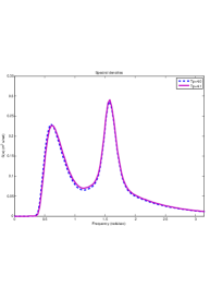
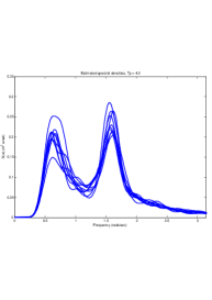
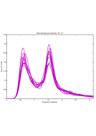
Figure 2: Torsethaugen spectra (left) and estimated spectral densities for $T_{p}=4.0$ (center) and $T_{P}=4.1$ (right).

From each simulation, the spectral density was estimated using a Parzen window with length 60. This was repeated 10 times for each of the two original spectral densities, yielding two independent samples of 10 functions each, which come from different populations. Due to the random variations in the simulation and estimation stages, these curves are similar in shape but present important variations. Figures 2 (center) and (right) show the two samples. These densities were represented using a b-spline basis of order 5 with 51 nodes in the interval $[0,\pi]$.

For testing whether the two samples come from the same distribution, two versions of the $Q_{n}$ statistic were considered. For the first one, the range of frequencies $[0,\pi]$ was divided into 8 intervals and the indicator functions of these intervals play the role of the $g$ functions. In this case, the score corresponding to a projection along the direction of one of these indicator functions is equivalent to integrating the energy for the range of frequencies represented by the interval. For the second version, a b-spline basis of order 5 with 7 interior nodes was used as $g$ functions. The values obtained for $Q_{n}$ for these two versions of the statistic were 39.105 and 120.18, respectively, with corresponding $p$-values, with respect to the asymptotic distribution, of $4.7\times 10^{-6}$ and 0. Nevertheless, taking into account the small sample sizes, asymptotic $p$-values cannot be considered valid and we must resort to Monte Carlo $p$-values. For this purpose, we use the fact that an algorithm is available for the generation of independent samples with a given spectral density. From the “original” set of 20 estimated spectral densities (10 for each parameter choice) an average spectral density was estimated, say $s_{\mbox{avg}}$. Then, $s_{\mbox{avg}}$ was used to produce two sets of 10 simulated stationary Gaussian random (wave) processes lasting 30 minutes, using the WAFO toolbox, as described above. From each 30 minute simulated wave process, the corresponding spectral density was estimated, to produce two sets of 10 spectral densities under the null hypothesis. On these two samples of spectral densities the statistic $Q_{n}$ was computed. The simulation procedure just described was repeated 10,000 times, using always the same $s_{\mbox{avg}}$, and the 10,000 values of $Q_{n}$ produced were used to estimate the $p$-value for the original value of the statistic. The resulting Monte Carlo $p$-values were 0.0492 and 0.0398, for the two schemes of $g$ functions considered, which shows that even for the small sample sizes considered and for two similar Torsethaugen spectral densities, the method proposed is able to produce some evidence of difference.

Next, we performed the same simulation experiment, with larger sample sizes, in order to assess speed of convergence to the limiting distribution. In this case we considered a sample size of 140 estimated spectral densities for $T_{p}=4.0$ and 160 for $T_{p}=4.1$. The $Q_{n}$ values for the sample were 507.03 for the indicator basis and 517.16 for the b-spline basis, with $p$-values equal to 0 in both cases. The Monte Carlo procedure is identical to the one described above for the smaller sample sizes and, in this case, from the Monte Carlo simulations, approximate quantiles were estimated, along with the Monte Carlo $p$-values. The results, regarding quantiles, for both versions of $Q_{n}$, are given in table 1.

Spline basis
Quantile	0.5	0.9	0.95	0.975	0.99
Asymptotic	11.34	18.549	21.026	23.337	26.217
MC	11.857	19.451	22.242	24.846	27.445
Rel. error	-0.046	-0.049	-0.058	-0.065	-0.047
Indicator basis
Quantile	0.5	0.9	0.95	0.975	0.99
Asymptotic	7.344	13.362	15.507	17.535	20.09
MC	7.443	13.819	16.064	18.202	20.892
Rel. error	-0.013	-0.034	-0.036	-0.038	-0.040

Table 1: Finite sample and limiting quantiles for the spectral density data.

The results in Table 1 show that the relative errors, between Monte Carlo and asymptotic quantiles, vary between 1.3 and 6.5% and are always negative, indicating that the asymptotic values underestimate the true quantiles of the statistic in this case. Thus, for this problem and the choices of functions $g$ made for $Q_{n}$, we conclude that the convergence to the limit distribution of the statistic is slow and it is advisable to calculate the necessary $p$-values using a Monte Carlo procedure.

4.2 Waves as functional data

The other two examples in this section concern the analysis of waves as real functions. The raw data consists of sea surface elevation measurements at a fixed point obtained from the U.S. Coastal Data Information Program (CDIP) website. The data come from buoy 106 (51201 for the National Data Buoy Center), a station located at Waimea Bay, Hawaii, at a sea depth of 200 meters. The surface elevation was sampled at a frequency of 1.28 Hz, during 30-minute intervals. A total of 430 intervals (8 days and 23 hours), between January 1${}^{\mbox{st}}$ and January 9${}^{\mbox{th}}$, 2003, were considered.

A wave is defined as the curve of surface elevation values between two consecutive downcrossings of the mean sea level (see Figure 1). For each 30-minute interval, the individual waves were considered as functions. Since the time length of each individual wave (the period) is different, all waves were registered to the $[0,1]$ interval by a linear transformation of the time interval. After registration, waves were initially represented using a B-spline basis of order 6 with nodes at the data points that define each wave. Then, these functions are represented using a common basis, again B-splines of order 6, but with 61 equidistant nodes on the interval $[0,1]$, so that all waves have a representation in terms of a common basis. The order of the splines guarantees that the functions are smooth, having two continuous derivatives.

Spectral densities were estimated for each 30-minute interval using the toolbox WAFO and the values of $\sigma^{2}$ and $H_{s}$ were obtained for each data interval. Figure 3 shows both the original sea surface elevation data and the evolution of $H_{s}$ in time.

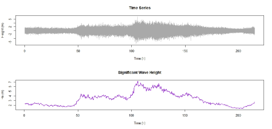
Figure 3: Wave height (top) and significant wave height (bottom) for Buoy 106.

For the purpose of evaluation of the methodology proposed here, the 30-minute intervals were divided into four groups, $G1,G2,G3$ and $G4$, according to the value of their significant wave height; the groups correspond to values in the ranges $0-2$ m., $2-4$ m., $4-6$ m. and values over 6 meters for $G4$.

Within each energy group, two consecutive 30-minute intervals were selected, and the waves corresponding to those intervals constitute the data set for the group. The selected sets of waves are indicated in Figure 3 (left) and are denoted in what follows as $H_{s}1$, $H_{s}2$, $H_{s}3$ and $H_{s}4$, with significant wave height increasing with numbering. The number of waves in each one-hour set are, respectively, 166, 171, 179 and 187. Figure 3 (right) shows the waves in the sets $H_{s}1$ to $H_{s}4$. It is clear that, in terms of amplitude, the waves in these groups are different, with the possible exception of $H_{s}3$ versus $H_{s}4$. We wish to quantify these differences with the methodology proposed in the previous section. We will compare, in the context of the two-sample problem, $H_{s}1$ versus $H_{s}2$, $H_{s}2$ versus $H_{s}3$ and $H_{s}3$ versus $H_{s}4$.

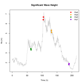
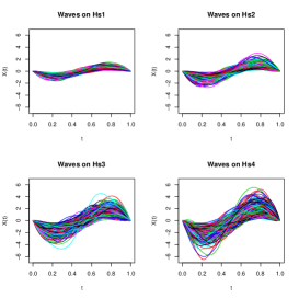
Figure 4: Position of selected intervals (left), waves in the selected time intervals (right).

4.3 Projection on odd and even trigonometric functions

For the problem of comparing the different data sets described in section 4.2, we apply the statistic $Q_{n}$, using two functions in the vector $\tilde{\mathbf{g}}$, that will be certain projections of the joint data set on linear combinations of the odd and even trigonometric functions with coefficients determined from the joint sample of functions. For each registered wave, $Z_{i}(t)$, in the joint sample, we consider its $l$-th sine and cosine Fourier coefficients, given by

$$a_{il}=\int_{0}^{1}Z_{i}(t)\sin(2\pi lt)\mbox{d}t\qquad\mbox{ and }\qquad b_{il}=\int_{0}^{1}Z_{i}(t)\cos(2\pi lt)\mbox{d}t.$$ (17)

We compute these coefficients for $l\leq k=3$, since the coefficients decrease very rapidly. For each $l\leq k$, we take the averages of the absolute values of the $a_{il}$ and $b_{il}$ as representatives of the relevance of the $l$-th term in the expansion:

$$\bar{a}_{l}=\frac{1}{N}\sum_{i=1}^{N}|a_{il}|\qquad\mbox{ and }\qquad\bar{b}_{l}=\frac{1}{N}\sum_{i=1}^{N}|b_{il}|,\qquad\mbox{ for }l=1,2\mbox{ and }3,$$ (18)

where, as before, $N=m+n$ is the size of the joint sample. Then, we take as our functions, $\tilde{g}_{1}$ and $\tilde{g}_{2}$, the following

$$\tilde{g}_{1}=\sum_{l=1}^{3}\bar{a}_{l}\sin(2\pi lt)\qquad\mbox{and}\qquad\tilde{g}_{2}=\sum_{l=1}^{3}\bar{b}_{l}\cos(2\pi lt).$$ (19)

These functions are calculated for each pair of energy levels: $H_{s}1$ versus $H_{s}2$, $H_{s}2$ versus $H_{s}3$ and $H_{s}3$ versus $H_{s}4$. As a reference, Table 2 shows the values of the coefficients that define $\tilde{g}_{1}$ and $\tilde{g}_{2}$ in the case of $H_{s}1$ versus $H_{s}2$ and Figure 5 shows the corresponding $\tilde{g}_{1}$ and $\tilde{g}_{2}$ functions plus a sine function for comparison purposes. Table 3 shows the values and $p$-values obtained when $Q_{n}$ is calculated for testing the difference of distribution between the groups of waves of different energy. Note that this time we evaluate the value obtained for $Q_{n}$ against the chi-square distribution with 2 degrees of freedom.

The numbers in Table 3 reflect very strong evidence against the null hypothesis in all cases, especially in the first two, as could be expected from the waveforms in Figure 4 (right), and these results also say that the projections on the trigonometric functions are enough, through the $Q_{n}$ statistic, for detecting the difference in energy between the samples.

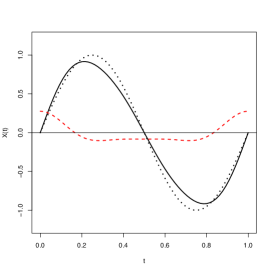
Figure 5: $\tilde{g}_{1}$ (solid), $\tilde{g}_{2}$ (dashed) and sine function (dotted) for the $H_{s}1$ vs. $H_{s}2$ test.

j	$\bar{a}_{j}$	$\bar{b}_{j}$
1	0.916	0.151
2	0.097	0.097
3	0.024	0.029

Table 2: Coefficients defining $\tilde{g}_{1}$ and $\tilde{g}_{2}$ for the $H_{s}1$ vs. $H_{s}2$ test.

Pair of samples tested	$Q_{n}$ value	$p$-value
$H_{s}1$ versus $H_{s}2$	103.75	0
$H_{s}2$ versus $H_{s}3$	107.37	0
$H_{s}3$ versus $H_{s}4$	17.01	2.02$\times 10^{-4}$

Table 3: $Q_{n}$ values for projections on odd and even trigonometric functions.

This result, however, is to be expected from the differences in amplitude that can be observed in Figure 4. So a natural question is whether the dissimilarities are only in amplitude, or whether there are also differences in the shape of the waves due to the variation in energy levels. To test if there are differences between these samples other than in amplitude, the normalized waves were considered, where the normalization was obtained dividing by the standard deviation estimated for each one-hour interval. We consider intervals $H_{s}1,H_{s}2$ and $H_{s}3$ and Figure 6 shows the registered waves for the three possible pairs of normalized samples. The differences among them, if there are any, are not so obvious now.

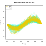
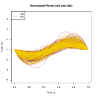
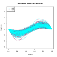
Figure 6: Waves in intervals $H_{s}1$ and $H_{s}2$ (left), $H_{s}1$ and $H_{s}3$ (center) and $H_{s}2$ and $H_{s}3$ (right).

Using the same method as before, the three pairs of samples were compared to test whether the curves come from the same distribution. The results of these tests are given in table 4, where the $p$-values obtained using the asymptotic distribution and a bootstrap procedure, described below, are included.

Pair of samples tested	$Q_{n}$ value	$p$-value (asymp.)	$p$-value (bootstrap)
$H_{s}1$ versus $H_{s}2$	17.15	$1.88\times 10^{-4}$	$4\times 10^{-4}$
$H_{s}2$ versus $H_{s}3$	1.023	0.5997	0.5997
$H_{s}3$ versus $H_{s}4$	2.258	0.323	0.333

Table 4: $Q_{n}$ and $p$-values based on principal components for the normalized samples.

These values show that the differences are not so clear after normalization, and point to the first interval $H_{s}1$ being different from the other three, but there is no evidence of differences between $H_{s}2$ and $H_{s}3$ or $H_{s}3$ and $H_{s}4$. Figure 7 shows the normalized spectra for these intervals, and may help explain the results obtained, since the spectral density of a time series sums up its oscillatory behavior. As can be seen, the spectra for intervals $H_{s}2$, $H_{s}3$ and $H_{s}4$ are similar in dominant frequency and dispersion while the spectrum for $H_{s}1$ is clearly different in both aspects. It is important to observe, however, that the process of registration of the individual waves to a common interval losses the information about the period of the wave, and hence also about frequency. Thus it seems likely that it is the dispersion (and shape) of the spectral density rather than its location in the frequency scale which accounts for the differences observed in the three samples. Nevertheless, the relationship between spectral densities and the shape of waves is not clear and requires further exploration.

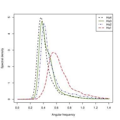
Figure 7: Spectral densities for intervals $H_{s}1,H_{s}2$ and $H_{s}3$.

Next, we evaluate whether, in this example, the asymptotic distribution as a reference is valid for the sample sizes considered. Thus, our next experiment evaluates, through a bootstrap procedure, the approximation to the null distribution in the present context. The bootstrap method used here does not require the estimation of spectral densities and, for this reason, is computationally significantly less expensive than the Monte Carlo procedure described before.

For this purpose, the 166 waves of data set $H_{s}1$ were used. The data were randomly split into two sets of 106 and 60 waves, respectively, and the $Q_{n}$ statistic was computed. This procedure was repeated for 10,000 random selections of the two subsets, of 106 and 60 waves (from the same joint sample of 166), calculating $Q_{n}$ every time. From the 10,000 values, we obtain quantiles of $Q_{n}$ that correspond, approximately, to the null hypothesis and are displayed in Table 5, were we have included, for comparison purposes, the corresponding quantiles for the $\chi_{2}^{2}$ distribution.

	Probabilities
	.5	.9	.95	.975	.99
asymptotic	1.386	4.605	5.992	7.378	9.21
bootstrap	1.365	4.662	6.147	7.454	9.169
relative error	0.0157	-0.0124	-0.0259	-0.0103	0.0045

Table 5: Finite sample and limiting quantiles of $Q_{n}$ for $H_{s}1$ data.

The good agreement between finite sample and limiting quantiles in Table 5, suggest that for sample sizes above a hundred for both samples, the proposed statistic can be confidently used for the type of data considered in this example. This form of bootstrap was used to produce the “bootstrap” quantiles in Table 4 by bootstrapping from the joint dataset in each case.

4.4 Asymmetry of real waves

One of the advantages of the set of statistics proposed in this work is its flexibility. In this section we show how it is possible to construct statistics suitable for the assessment of symmetry in samples of functions. In Gorrostieta et al. (2014), sets of registered storm waves were evaluated for asymmetry and also compared, by means of a conditional permutation test, to sets of waves generated from the Gaussian model with parameters estimated from the data. The Gaussian model, as described for instance in Ochi (1998), is a standard stochastic model for sea waves. Still, it was pointed out in the introduction that real waves differ from those produced by the model, in that real waves present more asymmetry than the model would allow, having shallower troughs and more peaked crests, and this difference may be more marked at higher energy levels.

We will now use the proposed statistic $Q_{n}$ to test for the null hypothesis that registered real waves and waves produced by the Gaussian model have the same distribution against the alternative that real waves show more asymmetry. For this purpose, we take a set of waves corresponding to two consecutive 30 minute period in each of the four energy levels considered in Section 4.2. For this analysis, in the registration process of the waves an added restriction was that the upcrossing of the mean level occurs at 0.5. The precise description of the registration procedure can be found in Gorrostieta et al. (2014). From each dataset, the spectral density is estimated and from it, a set of simulated waves is produced, using the WAFO toolbox of the MATLAB language. For each energy level, from the combined sample (real and simulated waves), we compute, for $l\leq 3$ and $i\leq N$, the coefficients $a_{il}$, the average $\bar{a}_{l}$ and the function $\tilde{g}_{1}$ of (17), (18) and (19). The idea is the following: The suspected asymmetry of real waves consists on the waves being less deep, in terms of amplitude, during the first half cycle, than the amount they rise above sea level on the second half cycle. This type of asymmetry should show in the dot product against a relevant odd function. Thus, we estimate a representative odd function $\tilde{g}_{1}$ and apply the statistic $Q_{n}$ with that function alone. If the alternative hypothesis holds, we expect that, for the real waves, the dot product with $\tilde{g}_{1}$ will have a positive mean value, while it will tend to zero for the simulated waves.

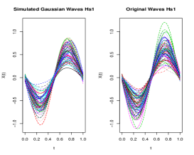
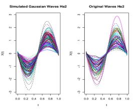
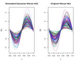
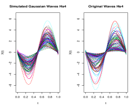
Figure 8: Real and simulated waves for the four groups considered.

Figure 8 shows the registered real waves and simulated waves considered for this symmetry test in groups $H_{s}1$ to $H_{s}4$. At first sight, in none of the cases is the asymmetry of the real waves evident.

Application of the procedure described above to the selected wave samples produced the results presented in Table 6. In this analysis the $p$-values are computed with the chi-square distribution with one degree of freedom, since a single function is used in the vector $\tilde{\mathbf{g}}$. At the first two energy levels, we find no evidence of the asymmetry, and in this sense, the mathematical model used seems to be producing waves similar to the real ones. At the higher energy levels, $H_{s}3$ and $H_{s}4$ the value of the statistic is significant at the 5% level, being much stronger the evidence for the $H_{s}4$ data. This results seem in agreement with what has been concluded in the literature by other means.

Energy level	Sample sizes (real $|$ simulated)	$Q_{n}$ value	$p$-value
$H_{s}1$	85 $|$ 78	2.69	0.101
$H_{s}2$	104 $|$ 156	0.31	0.578
$H_{s}3$	136 $|$ 127	4.87	0.027
$H_{s}4$	151 $|$ 121	51.58	6.9 $\times 10^{-13}$

Table 6: $Q_{n}$ values for asymmetry test

As a final remark, we conclude that the proposed methodology is a flexible tool that can be used to test the validity of different hypothesis on functional data sets.

5 Acknowledgements

The software WAFO (Brodtkorb et al., 2000) developed by the Wafo group at Lund University of Technology, Sweden, available at http://www.maths.lth.se/matstat/wafo was used for the calculation of all Fourier spectra and associated spectral characteristics as well as for the simulation of Gaussian random waves. The data for station 106 were furnished by the Coastal Data Information Program (CDIP), Integrative Oceanographic Division, operated by the Scripps Institution of Oceanography, under the sponsorship of the U.S. Army Corps of Engineers and the California Department of Boating and Waterways (http://cdip.ucsd.edu/). This work was partially supported by CONACYT, Mexico, Proyecto Análisis Estadístico de Olas Marinas, Fase II. It was finished while J.O. was visiting, on sabbatical leave from CIMAT and with support from CONACYT, México, the Departamento de Estadística e I.O., Universidad de Valladolid. Their hospitality and support is gratefully acknowledged.

References

- Benko et al. (2009) Benko, M., Härdle, W. and Kneip, A. (2009). Common functional principal components. Annals of Statistics 37: 1-34.
- Borgman (1972) Borgman, Leon E. (1972). Statistical Models for Ocean Waves and Wave Forces, In: Advances in Hydroscience Vol. 8, Ven Te Chow (Ed.), Academic Press, New York.
- Bosq (2000) Bosq, D. (2000). Linear Processes in Function Spaces. Lecture Notes in Statistics, Vol. 149, Springer, New York.
- Brodtkorb et al. (2000) Brodtkorb,P.A., Johannesson, P., Lindgren, G., Rychlik, I., Rydén, E. and E. Sjö (2000) WAFO - a Matlab toolbox for analysis of random waves and loads. In: Proc. 10th Int. Offshore and Polar Eng. Conf. (ISOPE). Vol. III, 343–350, Seattle, USA.
- Dudley (1987) Dudley, R.M. (1987) Universal Donsker Classes and Metric Entropy. Annals of Probability, 15: 1306–1326.
- Ferraty (2011) Ferraty, F. (Editor) (2011) Recent Advances in Functional Data Analysis and Related Topics. Physica Verlag, Berlin.
- Ferraty and Vieu (2006) Ferraty, F. and Vieu, P. (2006) Nonparametric Functional Data Analysis: Theory and Practice. Springer, New York.
- Gorrostieta et al. (2014) Gorrostieta, C., Ortega J., Quiroz, A. J. and Smith, G. H. (2014) Characterization of storm wave asymmetries with functional data analysis. Environmental and Ecological Statistics 21(2): 263-283.
- Hall and Van Keilegom (2007) Hall, P. and Van Keilegom, I. (2007). Two sample tests in functional data analysis starting from discrete data. Statistica Sinica 17: 1511-1531.
- Horváth and Kokoszka (2009) Horváth, L. and Kokoszka, P. (2009). Two Sample Inference in Functional Linear Models. Canadian Journal of Statistics 37: 571-591.
- Horváth and Kokoszka (2012) Horváth, L. and Kokoszka, P. (2012). Inference for Functional Data with Applications. Springer, New York.
- Longuet-Higgins (1956) Longuet-Higgins, M. (1956). Statistical properties of a moving wave form. Proc. Cambridge Philosophical Society 52 Part 2:234-245 .
- Longuet-Higgins (1957) Longuet-Higgins, M. (1957). The statistical analysis of a random moving surface. Philosophical Transactions of the Royal Society London, Series A 249(966):321 -387.
- Muñoz Maldonado et al. (2002) Muñoz Maldonado, Y., Staniswalis, J.G., Irwin, L.N. & Byers, D. (2002). A similarity analysis of curves. Canadian Journal of Statistics 30: 373-381.
- Ochi (1998) Ochi, M. K. (1998). Ocean Waves: The Stochastic Approach. Cambridge Ocean Technology Series. Cambridge University Press, Cambridge.
- Paparoditis and Sapatinas (2014) Paparoditis, E. & Sapatinas, Th. (2014). Bootstrap-based testing for functional data. arXiv:1409.4317v1 [math.ST].
- Peña (2012) Peña, J. (2012). Propuestas para el problema de dos muestras con datos funcionales. Tesis de maestría, Universidad de Los Andes, Colombia.
- Pierson (1955) Pierson, W. J. Jr. (1955). Wind-generated gravity waves. Advan. Geophys. 2: 93-178.
- Pollard (1982) Pollard, D. (1982) A Central Limit Theorem for Empirical Processes. Journal of the Australian Mathematical Society, Series A, 33: 235-248.
- Pollard (1984) Pollard, D. (1984) Convergence of Stochastic Processes. Springer, New York.
- Ramsay and Silverman (2002) Ramsay, J.O. & Silverman, B.W. (2002). Applied Functional Data Analysis. Springer, New York.
- Ramsay and Silverman (2005) Ramsay, J.O. & Silverman, B.W. (2005). Functional Data Analysis. 2nd. Edition Springer, New York.
- Torsethaugen (1993) Torsethaugen, K. (1993) A two-peak wave spectrum model. In Proc. 18th. Int. Conference on Ocean, Offshore and Artic Engineering (OMAE), Vol II, 175–180.
- Torsethaugen and Haver (2004) Torsethaugen, K. and Haver, S. (2004). Simplified double peak spectral model for ocean waves. In Proc. 14th. Int. Offshore and Polar Engineering Conference, 23–28.
- van der Vaart (1996) van der Vaart, Aad (1996) New Donsker Classes. Annals of Probability, 24: 2128-2140.
- van der Vaart (1998) van der Vaart, Aad (1998) Asymptotic Statistics. Cambridge University Press, Cambridge.
- van der Vaart and Wellner (1996) van der Vaart, A. W. and Wellner, J. A. (1996) Weak Convergence and Empirical Processes. Springer Series in Statistics. Springer, New York.