Effect of double local quenches on Loschmidt echo and entanglement entropy of a one-dimensional quantum system

Abstract

We study the effect of two simultaneous local quenches on the evolution of Loschmidt echo and entanglement entropy of a one dimensional transverse Ising model. In this work, one of the local quenches involves the connection of two spin-1/2 chains at a certain time and the other local quench corresponds to a sudden change in the magnitude of the transverse field at a given site in one of the spin chains. We numerically calculate the dynamics associated with the Loschmidt echo and the entanglement entropy as a result of such double quenches, and discuss various timescales involved in this problem using the picture of quasiparticles generated as a result of such quenches.

I Introduction

Recently, quantum information theoretic measures like decoherence haroche98 ; zurek03 ; joos03 , entanglement and fidelity dutta15 ; zanardi06 ; gu10 ; gritsev10 have become the subject of immense interest. Close to the quantum critical point (QCP) of a quantum many-body system, these quantities show peculiar behaviors and hence can be regarded as a tool to detect the QCP dutta15 . Decoherence that signifies the loss of coherence of the system when it interacts with the environment is an important observable for quantum computation.

In this context, Loschmidt echo (LE), which quantifies the decoherence is studied extensively quan06 ; zhang09 ; rossini07 ; sharma12 ; mukherjee12 ; nag12 ; rajak12 . The LE is defined as the square of overlap of the two wave functions $|\psi(t)\rangle$ and $|\psi_{0}(t)\rangle$ evolving with two different Hamiltonians $H$ and $H_{0}$, respectively, $i.e.,$

$$\mathcal{L}(t)=|\langle\psi(t)|\psi_{0}(t)\rangle|^{2}.$$ (1)

Initially, both the states are prepared in the ground state of $H_{0}$. LE provides information about how small perturbations during an evolution can result to the decoherence of the state of the system, thus being an important quantity for information processing and storage. On the other hand, LE can also be used to detect the presence of a QCP by showing a sharp dip at the QCP of the Hamiltonian when $H$ and $H_{0}$ are close to each other.

At the same time, the entanglement in quantum many-body systems, which is the measure of quantum correlations between the two systems, has also become a topic of intensive research interest for last several years osborne02 ; osterloh02 ; vidal03 ; korepin04 ; calabrese04 ; refael04 ; igloi08 ; song10 ; dubail11 . One of the quantities to measure the entanglement between the two subsystems is the von Neumann entropy holzhey94 ; amico08 ; calabrese09 ; eiser10 . Consider a bipartite system divided into two subsystems $A$ and $B$ of length $L_{A}$ and $L_{B}$ with total length $L=L_{A}+L_{B}$. If the whole system is in a quantum pure state $|\psi\rangle$ with density matrix $\rho=|\psi\rangle\langle\psi|$, then the von Neumann entropy $S$ of system A with reduced density matrix $\rho_{A}={\rm Tr}_{B}(\rho)$ is defined as

$$S=-{\rm Tr}(\rho_{A}\log\rho_{A}).$$ (2)

The entanglement entropy (EE) or $S$ increases with increasing quantum correlations (entanglement) between the two subsystems. EE exhibits distinct scaling relations at and close to a quantum critical point with the shortest length scale of the system. For a critical spin chain with periodic boundary conditions where the subsystem has two boundary points, the entanglement entropy scales as $S=\frac{c}{3}\log L_{A}$, where $c$ is a universal quantity and given by the central charge of the conformal field theory holzhey94 ; vidal03 ; calabrese04 . On the other hand, away from the critical point where the correlation length $\xi\ll L_{A}$, entanglement entropy is given by $S=\frac{c}{3}\log\xi$. The above scaling relations are valid for a one-dimensional homogeneous system. It is found that some modifications are required in the scaling relations of EE when the system is inhomogeneous. Interestingly, in this case also the scaling relations remain same as the homogeneous case with a changed prefactor $c_{\rm eff}$ which is called the effective central charge refael04 ; laflorencie05 ; chiara06 ; refael07 ; bonesteel07 ; igloi07 ; igloi071 .

With our understanding of behavior of EE in an equilibrium system getting better, a considerable amount of focus is also given to EE in systems out of equilibrium calabrese05 ; eisler07 ; calabrese07 ; eisler08 ; igloi09 ; hsu09 ; cardy11 ; stephan11 ; igloi12 . The experimental demonstration of such non-equilibrium dynamics using optical lattices bloch08 also contributes to the sudden upsurge in studies related to decoherence and entanglement in out of equilibrium systems. One of the ways of generating such a non-equilibrium dynamics is a sudden quench. A sudden quench in the system can be performed locally or globally. In a global quench, a parameter of the Hamiltonian is changed suddenly at all the sites resulting to a non-equilibrium dynamics. In this process, EE generally shows a linear increase in time $t$ up to some time $t_{0}$ calabrese05 . The local quench is defined as a local change of a parameter of the Hamiltonian. For example, the entanglement entropy between two critical subsystems $A$ and $B$ of a homogeneous one-dimensional chain which are disconnected for $t<0$ and connected at $t=0$ increases as $S=\frac{2c}{3}\log t$ for $t\ll L$ eisler07 ; calabrese07 ; stephan11 ; here the final chain is periodic. On the other hand, if the final chain is open, the factor $2$ in the expression of $S$ is not present. Such studies are important in the context of information propagation through a quantum many body system.

In this paper, we consider two independent transverse field Ising spin chains in the ferromagnetic or critical phase. For the times $t<0$, the two spin chains which are in their respective ground states, are disconnected and are later joined at $t=0$ ($J$-quenching). Simultaneously, we change the magnitude of the transverse field at a single site of one of the chains ($h$-quenching). This results to a non-equilibrium evolution of the state of the system. If we consider only $J$-quenching of a critical Ising chain, both the quantities, namely, LE and EE show periodic time evolution stephan11 . However, in this paper, we address the effect of $h$-quenching along with the $J-$quenching in critical and off-critical systems which results to a non-trivial evolution of LE and EE when compared to the no $h$-quenching case. We shall try to understand these results using the picture of quasiparticles generated due to both the local quenches. Our most significant observation here is the reflection of the quasiparticles at the site of $h$-quenching. We find some interesting time scales in the evolution of both LE and EE when the two quenches are performed simultaneously. These timescales can be explained successfully using the reflection picture of the quasiparticles generated. We have also argued qualitatively how the evolution of EE changes as the total system moves from deep ferromagnetic phase to critical one.

The organization of the paper is as follows: we discuss the model studied in this paper along with briefly mentioning the numerical techniques in section II.1 followed by a discussion on semiclasscial theory of quasiparticles generated in section II.2. In section III, we present the results of LE and EE in the critical region for various geometries whereas we present the results for the ferromagnetic region in section IV. A comparison between the two quenches studied in this paper is made in section V using the semiclassical picture. We conclude this paper with our main results in section VI. We have also added two appendices at the end of the paper outlining the numerical techniques used in this paper.

II Model

II.1 Exact diagonalization

The Hamiltonian we consider here is that of a one-dimensional Ising chain in a transverse field given by

$$H~{}=~{}-\sum_{n}(J_{n}\sigma_{n}^{x}\sigma_{n+1}^{x}~{}+~{}h_{n}\sigma_{n}^{z}),$$ (3)

where $h_{n}$ and $J_{n}$ are the site dependent transverse magnetic fields and cooperative interactions, respectively, and $\sigma^{x}_{n}$ and $\sigma^{z}_{n}$ are standard Pauli matrices at the lattice site $n$. For the homogeneous case ($h_{n}=h$ and $J_{n}=J$), the model in Eq. (3) has a QCP at $J=h$ separating ferromagnetic and quantum paramagnetic phases. Using Jordan-Wigner transformations followed by Fourier transformation for a homogeneous and periodic chain, the energy spectrum for the Hamiltonian (3) is obtained as lieb61 ; pfeuty70

$$\varepsilon_{q}=\pm 2J\sqrt{(h+\cos q)^{2}+\sin^{2}q},$$ (4)

where $q$ is the momentum which takes discrete values given by $q=2\pi m/L$ with $m=0\cdots L-1$ for a finite system of length $L$.

On the other hand, such homogeneous systems are very rare in nature. One atleast finds some local defects, no matter how pure the material is. The general method adopted to study systems which are not homogeneous is outlined below, which we also use in this paper. Following Jordan-Wigner transformation, the Hamiltonian in Eq. (3) can be described by a quadratic form in terms of spinless fermions $c_{i}$ and $c_{i}^{\dagger}$ lieb61

$$H=\sum_{i,j}\left[c_{i}^{\dagger}A_{i,j}c_{j}+\frac{1}{2}(c_{i}^{\dagger}B_{i,j}c_{j}^{\dagger}+\mathrm{h.c.})\right].$$ (5)

Here, $\mathbf{A}$ is a symmetric matrix due to hermicity of $H$ and $\mathbf{B}$ is an antisymmetric matrix which follows from the anticommutation rules of $c_{i}$’s. The elements of these matrices thus obtained are:

$$A_{i,j} = -(J_{i}\delta_{j,i+1}+J_{j}\delta_{i,j+1})-2h_{i}\delta_{i,j},$$ (6)

$$B_{i,j} = -(J_{i}\delta_{j,i+1}-J_{j}\delta_{i,j+1}).$$ (7)

The above Hamiltonian can be diagonalized in terms of the normal mode spinless Fermi operators $\eta_{k}$ given by the relation lieb61 .

$$\eta_{k}=\sum_{i}(g_{k}(i)c_{i}+h_{k}(i)c_{i}^{\dagger}),$$ (8)

where $g_{k}(i)$ and $h_{k}(i)$ are real numbers. In terms of these operators the Hamiltonian takes the diagonal form,

$$H=\sum_{k}\Lambda_{k}\left(\eta_{k}^{\dagger}\eta_{k}-\frac{1}{2}\right),$$ (9)

with $\Lambda_{k}$ being the energy of different fermionic modes with index $k$. These $\Lambda_{k}^{\prime}s$ are given by the solutions of the eigenvalue equations,

$$(\mathbf{A}-\mathbf{B})(\mathbf{A}+\mathbf{B})\mathbf{\Phi}_{k} = \Lambda_{k}^{2}\mathbf{\Phi}_{k}$$ (10)

$$(\mathbf{A}+\mathbf{B})(\mathbf{A}-\mathbf{B})\mathbf{\Psi}_{k} = \Lambda_{k}^{2}\mathbf{\Psi}_{k}\;.$$ (11)

It can be shown that the elements of the eigenvectors are related to $\mathbf{g}$ and $\mathbf{h}$ matrices used to diagonalize the Hamiltonian as follows: $\Phi_{k}(i)=g_{k}(i)+h_{k}(i)$ and $\Psi_{k}(i)=g_{k}(i)-h_{k}(i)$. We calculate LE and EE using $\Phi$, $\Psi$, $\mathbf{g}$ and $\mathbf{h}$ as discussed in appendices A, and B.

II.2 Semiclassical theory of quasiparticles

When a system at zero temperature is taken away from its ground state by applying some perturbation, the state of the system undergoes a non-equilibrium evolution with respect to the final Hamiltonian. The initial state, which now is an excited state, is a source of quasiparticles (QPs) corresponding to the final Hamiltonian. Recently, such non-equilibrium dynamics have been studied using a semiclassical picture of quasiparticles generated for global rieger11 ; blass12 and local quenches divakaran11 , where excellent agreement between the numerics and the semiclassical theory were obtained. We now briefly describe this theory of quasiparticles generated which shall be used to explain the various timescales observed in our numerical calculations. For global quenches from $h=0$ to a very small $h$ value, it can be shown that these quasiparticles are wavepackets of low-lying excitations and discussed in details in Ref. rieger11 . Due to the conservation of momentum, quasiparticles of a given momentum are always produced in pairs, the group velocity $v_{g}(k)(=|\partial\varepsilon_{k}/\partial k|)$ of them being equal and opposite to each other. As discussed in Ref. rieger11 , these quasiparticles in the small $h$ limit can be considered as classical particles (sharply defined QPs) which when crosses a site, simply flips the spin at that site. Though this picture is discussed for a very specific quench (a small quench), it has been verified for stronger quenches and also for quenches in the paramagnetic phase with slight modifications. It is also argued that these quasiparticles are no longer point particles, but are extended objects as the critical point is approached due to large correlation length. In the following sections, we shall try to explain our numerical results atleast qualitatively with this point like picture of quasiparticles for spin chains in the ferromagnetic as well as in the critical region.

III Loschmidt echo and Entanglement entropy for critical chain

We first study double quenches for a critical chain where already some work has been done in Ref. stephan11 ; calabrese07 for local J-quenches. As discussed before, we consider simultaneous application of two types of local perturbations to the system and study the time evolution of Loschmidt echo (LE) and von Neumann entanglement entropy (EE) as a result of such quenches. Initially the spin chain is prepared in the ground state of $H=H_{1}$ + $H_{2}$ where $H_{1}$ and $H_{2}$ are the Hamiltonians of two decoupled homogeneous Ising chains of length $L_{1}$ and $L_{2}$, respectively, with open boundary conditions ($J_{L_{1}}=J_{L_{2}}=0$). Two simultaneous quenches are performed at $t=0$, namely, (i) the two spin-1/2 chains are suddenly connected together resulting to a chain of total length $L=L_{1}+L_{2}$, and, (ii) the transverse field at a particular site $L^{\prime}$ belonging to either the chain $1$ or $2$ is changed from $h$ to $h+\delta$. The system then evolves with the final Hamiltonian

$$H_{f}=H_{1}+H_{2}+H_{12}^{I}-\delta\sigma^{z}_{L^{\prime}},$$ (12)

where $H_{12}^{I}$ defines the connection between the two spin chains of length $L_{1}$ and $L_{2}$ and is of the form $J\sigma^{x}_{L_{1}}\sigma^{x}_{L_{1}+1}$. At the same time, the term $-\delta\sigma^{z}_{L^{\prime}}$ in the Hamiltonian corresponds to the $h-$quenching which changes the magnitude of transverse field at site $L^{\prime}$ from $h$ to $h+\delta$. We incorporate these quenches numerically by considering a single spin chain of total length $L=(L_{1}+L_{2})$ with the first $L_{1}$ spins forming the system 1 and the remaining system 2. They are disconnected at $t<0$ by putting $J_{L_{1}}=0$ which at $t=0$ is then increased to $J$, also the interaction strength at all the other sites. For all our calculations, we have set $J=1$. The details of the numerical calculations for LE and EE are outlined in the appendix, see also Refs. [rossini07, ; igloi09, ].

As we switch on the two local perturbations discussed above, there is a local increase in energy of the system at the site of local perturbations calabrese07 ; divakaran11 . These sites then become the source of quasiparticle production. Henceforth, we shall call the quasiparticles created due to the $h$-quenching at $L^{\prime}$ as $QP^{1}$ , and the corresponding left and right moving quasiparticles as $QP^{1}_{L}$ and $QP^{1}_{R}$, respectively. Similarly, the left and right moving quasipartciles created at the site $L_{1}$ of $J-$quenching shall be called as $QP^{2}_{L}$ and $QP^{2}_{R}$. Below, we present our results for the evolution of LE and EE for various cases or geometry and discuss these results in the light of quasiparticles propagating in the system.

\begin{overpic}[width=213.39566pt]{LE_lcl2_deltal3} \put(-4.0,45.0){$\mathcal{L}(t)$} \end{overpic}

Figure 1: The plot shows LE as a function of time for different values of $\delta$ with $J-$quench at $L_{1}=L/2$ and the $h-$quench at site $L^{\prime}=L/3$. The transverse field at $L^{\prime}$ is changed from $1$ to $1+\delta$. For the $J$ quenching alone (i.e., $\delta=0$ case), the LE shows peak at $t_{3}=L/v_{\text{max}}=150$ and $T=2t_{3}$ where $v_{\text{max}}=2$ and $L=300$. By applying two local perturbations simultaneously at time $t=0$, we observe a small peak at $t^{\prime}=50$ and comparatively a stronger peak at $t^{\prime\prime}=200$. We also note small fluctuations near $t_{1}=100$ which is more clearly seen for $\delta=1$ curve.

III.1 LE and EE for $L_{1}=L_{2}$

In this section, we consider $J-$quenching at $L_{1}=L_{2}=L/2$ and the $h$-quenching at some site $L^{\prime}$ of the total spin chain of length $L$ at time $t=0$. Let us first discuss the dynamics of LE. In general, for the better readability of the paper, we shall assume $L^{\prime}<L_{1}\leq L_{A}$ (explained later in the context of EE) through out the paper but the case with $L^{\prime}>L_{1}$ is also presented and discussed in the caption of various figures. Due to the propagation of the generated quasiparticles, we expect four time scales which are the times of come back of the quasi-particles at the source point after getting reflected from boundaries of the chain, thus removing the effect of their dynamics. When this happens, the overlap in the definition of LE increases and shows a peak. These time scales are determined by the fastest moving QPs with maximal group velocity $v_{\text{max}}=\text{max}_{k}~{}v_{g}(k)$ and are given by $t_{1}=(2L^{\prime})/v_{\text{max}}$ (time of come back of $QP^{1}_{L}$), $t_{2}=2(L-L^{\prime})/v_{\text{max}}$ (time of come back of $QP^{1}_{R}$), $t_{3}=(2L_{1})/v_{\text{max}}$ (time of come back of $QP^{2}_{L}$) and $t_{4}=(2L_{2})/v_{\text{max}}$ (time of come back of $QP^{2}_{R}$). With $L_{1}=L_{2}$, the values of $t_{3}$ and $t_{4}$ are equal, but it is not the case in general. Other than the above mentioned obvious time scales, two more time scales are observed numerically, $t^{\prime}$ given by $2|L_{1}-L^{\prime}|/v_{\text{max}}$, which appears to be the time taken by $QP^{2}_{L}$ (for $L_{1}>L^{\prime}$) to reach $L^{\prime}$ and get partially reflected at $L^{\prime}$ where it finds a change in potential from $h$ to $h+\delta$. The second time scale is same as $t_{2}$, but it is due to $QP^{2}$ and is given by $t^{\prime\prime}=2(L-L^{\prime})/v_{\text{max}}$, which is the time taken by the $QP^{2}_{L}$ ($QP^{2}_{R}$) to get reflected at $L^{\prime}$ (right boundary) and come back to $L_{1}$ after getting fully (partially) reflected at the right boundary ($L^{\prime}$). It is to be noted that $v_{\max}$ for the homogeneous transverse Ising model with elements as defined in Eq. 7 is $2$ at the critical point and also in the paramagnetic phase. We shall use the same value of $v_{\max}$ in our case also since the numerically obtained value of $v_{max}$ by differentiating the eigenvalues is also close to 2.

\begin{overpic}[width=213.39566pt]{LE_lcl2_delta_1} \put(-4.0,45.0){$\mathcal{L}(t)$} \end{overpic}

Figure 2: The plot shows LE as a function of time when $h$-quenching of strength $\delta=1.0$ is performed at different sites $L^{\prime}$ of the total chain with $J$-quenching fixed at $L_{1}=L/2$. Here $L^{\prime}=0$ corresponds to the case of $J$-quenching alone where $t_{3}=t_{4}=150$. For $L^{\prime}=L/3$ ,$t^{\prime}=50$ and $t^{\prime\prime}=200$ whereas $t^{\prime}=90$ and $t^{\prime\prime}=240$ for $L^{\prime}=L/5$. All these timescales are clearly seen in the above figure. We also observe small perturbations at $t_{1}$ which is not very clear.

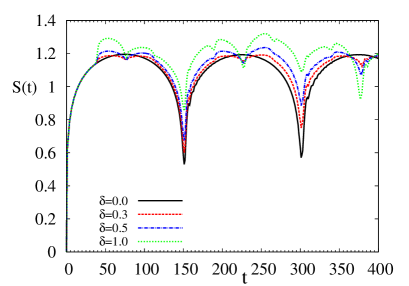
Figure 3: Entanglement entropy as a function of time after a local $J$-quench in the middle of the chain ($L_{1}=L/2$) along with $h$-quenching at $L^{\prime}=L/4$ for different interaction strengths $\delta$. Here, we consider $L_{A}=L_{1}=L/2$ as the subsystem with total system size $L=300$. The time scales $t^{\prime}/2$, $t^{\prime}$ and $t^{\prime\prime}$ can be seen in this figure which agrees well with our explanations. In this case, $t^{\prime}=75$ and $t^{\prime\prime}=225$. Another time scale observed is around $t=187$ which is when $QP^{1}_{R}$ enters system A resulting to an increase in EE as $QP^{1}_{L}$ is in system B during that time. Note that the effect of $QP^{1}$ is very small compared to $QP^{2}$.

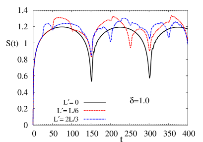
Figure 4: Time evolution of entanglement entropy after a local $J$-quench with $h$-quenching at different sites $L^{\prime}$ for $\delta=1.0$. For $L^{\prime}=L/6=50$, the deviation from the no $h$-quench case starts at $t^{\prime}/2=50$. A sharp decrease is observed at $t=t^{\prime}=100$ when $QP^{2}_{L}$ gets reflected at $L^{\prime}$ and returns to $L_{1}=L_{A}$. There is a sudden increase in EE after $t=150$ when $QP^{2}_{R}$ enters system A whereas $QP^{2}_{L}$ is still in system B. We again see a dip at $t^{\prime\prime}=250$ when $QP^{2}_{L}$ and $QP^{2}_{R}$ exchange their systems. Similarly, for the case $L^{\prime}=2L/3=200$, $QP^{1}_{L}$ enters system A at $t=t^{\prime}/2=25$ when the deviation from the single quench case appears. We see a sudden decrease of EE at $t=t^{\prime}$ when $QP^{2}_{R}$ enters system A after getting reflected at $L^{\prime}$ so that both the quasiparticles are in system A. After $t=150$, once again EE increases as $QP^{2}_{L}$ enters system B. A sharp dip is seen at $t=t^{\prime\prime}=200$ when $QP^{2}_{L}$ and $QP^{2}_{R}$ exchange systems.

We show the evolution of LE in Fig. 1 for different values of $\delta$. Let us first concentrate on the results of LE with $\delta=0$. Since LE is the overlap of two wavefunctions which had unity overlap initially, it starts decreasing from one at $t=0$ till both the quasiparticles reach the boundary at $t=L/4$ (since $L_{1}=L_{2}=L/2$ and $v_{\max}=2$), where it gets reflected. Intuitively, during its return path, QPs will undo their effect of dynamics. Thus, we expect to see a decrease in LE till the reflection of the first quasiparticle ($i.e.,$ till t=L/4) after which there is an increase till the quasiparticle reaches its origin or till $t=L/2(=2L_{1}/2)$. After this time, the initially left (right) moving quasiparticle will move to the system 2 (system 1) and eventually come back to its origin showing a peak at $t=T=L$, which is also the time period of the quasiparticles, see Fig. 1. When the second quench or the h-quench is also performed simultaneously, we expect to see some structures close to the time scales mentioned before, i.e., at $t_{1},t_{2},t^{\prime},t^{\prime\prime}$ along with the $\delta=0$ structure. The numerical results of such double quenches are shown in Fig. 1 for various coupling strengths $\delta$ and fixed $L^{\prime}$. As expected, the decay in LE is stronger with increasing strength of the local h-quench or $\delta$. On the other hand, Fig. 2 shows the variation of LE$(t)$ when the $h$-quench is performed at different positions of the chain with fixed $\delta=1$ demonstrating the above mentioned time scales more clearly, especially the variation of $t^{\prime\prime}$ with $L^{\prime}$. We find good agreement between the timescales proposed above and the numerics, see the caption for more details.

In conclusion, we find that the dominant peaks are due to $QP^{2}$ at times $t^{\prime},t^{\prime\prime},t_{3}$ and $t_{4}$, where $t_{3}=t_{4}$ in this case. We also note that the peak at $t^{\prime\prime}$ is a strong peak which may be due to the fact that at this time three different quasiparticles return to their origin after reflections at various points as discussed below: (i) $QP^{1}_{R}$ after reflection from the right boundary, (ii)$QP^{2}_{R}$ after reflection from right boundary and a second reflection at $L^{\prime}$ causing it to return to $L_{1}$ (iii) $QP^{2}_{L}$ after reflection at $L^{\prime}$ and a second reflection at right boundary resulting to its return to $L_{1}$. Finally, a peak is also observed at $t=L$ which is the return time of all the fastest quasiparticles back to their origin when there is no reflection at $L^{\prime}$, thus giving us a hint that there may be a transmitted component of the quasiparticle also. We shall comment more on it after discussing the results in the ferromagnetic phase.

It is to be noted that the presence of time scale $t_{1}$ due to $QP^{1}$ is almost negligible in these figures, though we do observe some perturbation at this time. On the other hand, it is too early to discard the presence of $QP^{1}$ as its effect is very clearly observed in the evolution of EE as explained in the next paragraph, thus ruling out the possibility of absence of such quasiparticles. We shall try to argue about the absence of $t_{1}$ scale in the evolution of LE in section V.

We now focus on the entanglement entropy as a function of time for the above scenario. In this case, another parameter is the size $L_{A}$ of system A of which we calculate the entanglement entropy with the remaining system of size $L-L_{A}$. Let us first consider the simplest case where $L_{1}=L_{A}$, i.e., the location of J-quenching also determines the size $L_{A}$ of system A. Interestingly, the bipartite EE of two critical transverse Ising chains can also detect the response of $h$-quenching (see Fig. 3, 4). We see that for $J$ quenching alone or for the single quench, the entanglement entropy shows perfect periodic oscillations with dips at $t_{3}=t_{4}=2L_{1}/v_{\max}$, also discussed in Ref.stephan11 using conformal field theory. This can also be explained using the quasiparticle picture. A pair of quasiparticle will increase the entanglement between the system A and the rest if one of them is in system A and the other is in B. The quasiparticle pairs are generated at $L_{1}=L_{A}=L/2$ and travel in opposite directions resulting to an immediate increase in $S(t)$ for $t>0$. This is not the case when $L_{1}\neq L_{A}$ and will soon be discussed separately. As both of them reaches the boundary at $t=L/4$ and gets reflected, $S$ starts decreasing and eventually shows a dip when $t=L/2$ after which both the quasiparticles belonging to a pair exchange their systems and once again EE increases after $t=L/2$. At $T=2L/v_{\text{max}}(=L)$, both the quasiparticles arrive at the starting point and $S$ shows a dip once again after which the pattern repeats. This is also shown in Fig 4 with $L^{\prime}=0.0$. If we now perform local $h$-quenching at a general site $L^{\prime}$ of the spin chain, we observe that the evolution of EE in double quenches follows the single quench case but accompanied by deviations at certain times which can once again be explained using the quasiparticle picture. We observe that the double quench case follows the single quench case $(\delta=0.0)$ till $t=t^{\prime}/2$ after which there is a sudden deviation or increase from the single quench case. This is because one of the quasiparticles ($QP^{1}_{R}$) produced at $L^{\prime}$ (which is not present in single quench case) enters the system B at this time whereas the other quasiparticle of the same pair remains in system A. This results to an extra increase in $S$. On the other hand, at $t=t^{\prime}$, the $QP^{2}_{L}$ reaches back to $L_{1}=L_{A}$ after reflection at $L^{\prime}$ where we find a sharp decrease in $S$ as both $QP^{2}_{L}$ and $QP^{2}_{R}$ are now in system B. The EE keeps on decreasing (after a slight increase) till $QP^{2}_{R}$ enters system A at $t=2(L-L_{1})/v_{\max}$ as a result of getting reflected from the right boundary, after which we observe a sharp increase in EE. One more time scale observed corresponds to $t^{\prime\prime}=2(L-L^{\prime})/v_{\max}$ which was also observed in LE. At this time, the $QP^{2}_{R}$ and $QP^{2}_{L}$ return back to $L_{A}$ and exchange their systems, as also discussed before with reference to LE.

The main difference between the analysis of LE and EE is that in the case of LE, we are interested in time scales at which the produced quasiparticles come back to its origin. In the case of EE, we are interested in the timescales in which one of the quasiparticles belonging to a pair crosses one system and goes to the other system. If this crossover results to both the QPs to be in the same system, then EE decreases, otherwise it increases Here, since we considered the geometry where $L_{1}=L_{2}=L_{A}$, many of the time scales are hidden. In the next section, we apply the same ideas to the case when $L_{1}\neq L_{2}$ but $L_{1}=L_{A}$ along with a special discussion for the most general case when $L_{1}\neq L_{2}\neq L_{A}$, and verify the quasiparticle picture proposed.

\begin{overpic}[width=213.39566pt]{LE_lcl3_delta_1} \put(-4.0,45.0){$\mathcal{L}(t)$} \end{overpic}

Figure 5: The plot shows LE as a function of time for double quenches with $L_{1}=100,L_{A}=100$ and $L=300$ and different $L^{\prime}$. The first peak of LE occurs at time $t^{\prime}=2(L_{1}-L^{\prime})/v_{\max}$ ($t^{\prime}=25$ and $50$ for $L^{\prime}=L/4$ and $L/6$ respectively). The other time scales are $t_{3}=100$, $t_{4}=200$ and $t^{\prime\prime}$. We note that $t^{\prime\prime}=225$ and $250$ for $L^{\prime}=75$ and $50$, respectively.

III.2 LE and EE for $L_{1}\neq L_{2}$

We are now interested in the local quenching of asymmetric spin chain ($L_{1}\neq L_{2}$). Let us first study the evolution of Loschmidt echo. For $J$-quenching alone stephan11 , the LE shows three time scales given by $t_{3}$, $t_{4}$ and the time period $T$ discussed in section III.1 (see $L^{\prime}=0$ plot of Fig. 5). The nature of these plots are discussed in details in Ref. stephan11 using conformal field theory. When the transverse field term at $L^{\prime}$ is changed from $h$ to $h+\delta$ together with J-quenching, we expect to see the following additional time scales in parallel with the discussion in the previous section: $t_{1}=(2L^{\prime})/v_{\max}$, $t^{\prime}=2(L_{1}-L^{\prime})/v_{\max}$ , $t^{\prime\prime}=2(L-L^{\prime})/v_{\max}$ Fig. 5 shows LE as a function of time after $J$-quenching at $L_{1}=L/3$ and $h$-quenching at different sites $L^{\prime}$. All the above mentioned time scales can be clearly seen in this figure except $t_{1}$. We shall try to argue for this latter.

Let us now move on to the calculation of EE for the same situation ($L_{1}\neq L_{2}$, but $L_{1}=L_{A}$). Fig. 6 shows the time evolution of EE after single and double quenching at time $t=0$. One can observe the difference in LE and EE between the times $t_{3}$ and $t_{4}$ for $\delta=0$ case (see Fig. 5 and Fig. 6). In this time range LE remains constant. On the other hand EE decreases slowly and then starts increasing at $t=t_{4}$ as discussed in Ref. stephan11 , the increase being due to arrival of $QP^{2}_{R}$ in system A. Moving to the double quenches, the discussion is almost same as for the case $L_{1}=L_{2}=L/2$ in the previous section. EE more or less follows the $\delta=0$ case and we see special time scales at $t^{\prime}/2$, $t^{\prime}$ and $t^{\prime\prime}$. See caption of Fig. 6 for more details.

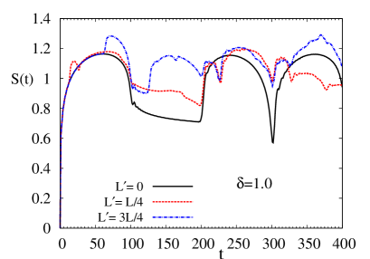
Figure 6: Time evolution of entanglement entropy for the same case as in Fig. 5 but different $L^{\prime}$. For $L^{\prime}=L/4$, the deviation from single J-quench case appears at $t^{\prime}/2=12.5$ whereas at $t^{\prime}=25$, $QP^{2}_{L}$ enters system B after getting reflected at $L^{\prime}$ where its other partner $QP^{2}_{R}$ is already present. The decrease in EE continues till $QP^{2}_{R}$ enters system A at $t=L_{2}=200$. We also see a dip at $t=t^{\prime\prime}=225$ where $QP^{2}_{L}$ and $QP^{2}_{R}$ exchanges their systems. Similarly, one can argue for the evolution of EE when $L^{\prime}=3L/4$. The deviation from the single quench case begins at $t=62.5$. In this case, $QP^{2}_{L}$ enters system B at $t=100$ which causes a sharp decrease at this time. On the other hand, $QP^{2}_{R}$ enters system A at $t=125$ resulting to an increase in EE as its other counterpart is still in B. The natural increase at $t=200$ which is there for only J-quenching case can also be observed. This might be due to the fact that any reflection at $L^{\prime}$ is not perfect and there is a possibility of getting a transmitted component of the QP wave, also discussed in sections IV and VI. The time scales $t^{\prime\prime}=225$ and $T=300$ are also present.

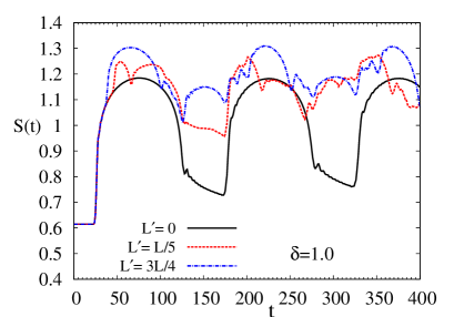
Figure 7: Time evolution of entanglement entropy after a local $J$-quenching at $L_{1}=L/3$ and $h$-quenching at different sites $L^{\prime}$ with $\delta=1.0$. Here, the subsystem is of length $L_{A}=L/2$ which does not coincide with cut resulting to few more relevant time scales. For $L^{\prime}=L/5=60$, the first deviation (or increase) from the single quench case appears at $t=45$. The EE decreases at $t=t^{\prime}=65$ when $QP^{2}_{L}$ and $QP^{2}_{R}$ are in the same subsystem B. The next increase in EE would be at $t=175$ when $QP^{2}_{R}$ enters subsystem A. The split of time scale $t^{\prime\prime}$, as discussed in the text, can also be seen with dips at $t^{\prime\prime}_{1}=215$ and $t^{\prime\prime}_{2}=265$. The case with $L^{\prime}=3L/4$ is all the more interesting. The deviation occurs at $t=(L^{\prime}-L_{A})/2=37.5$. The sharp decrease in this case occurs at $t=100$ which is the time taken by $QP^{2}_{R}$ to get reflected at $L^{\prime}$ and enter system A so that both $QP^{2}_{R}$ and $QP^{2}_{L}$ are in system A. But at $t=125$, $QP^{2}_{L}$ enters system B after getting reflected from the left boundary resulting to an increase in EE. $t^{\prime\prime}_{1}=200$ (due to $QP^{2}_{L}$) and $t^{\prime\prime}_{2}=250$ (due to $QP^{2}_{R}$). We note extra dips around $t=187$ which seems to be due to $QP^{1}_{L}$ entering system B after reflection from the left boundary.

We now consider the most general situation with $L_{1}\neq L_{2}\neq L_{A}$ and calculate the time evolution of EE. Here, $J$-quenching is again performed at $L_{1}$, but the subsystem is assumed to be of length $L_{A}=L/2$, different from $L_{1}$. The EE as a function of time after the double quenches is shown in Fig. 7. Let us define $l(=L_{A}-L_{1})$ as the distance between the right end of the subsystem A and the site of $J$-quenching. As in other cases, we discuss explicitly the case with $L^{\prime}<L_{1}<L_{A}$ below, and try to present some other examples through the figures. For $\delta=0$, EE remains at a constant value for small times and starts increasing at $t=l/v_{\max}$ when $QP^{2}_{R}$ hits at the boundary of the two subsystems and enters the subsystem $B$  eisler07 . Note the contrast between $L_{1}=L_{A}$ where $S(t)$ increases immediately and $L_{1}\neq L_{A}$ where $S(t)$ is constant initially. The EE shows a sharp decrease at $t=(2L_{1}+l)/v_{\max}$ when $QP^{2}_{L}$ enters system B after getting reflected from the left boundary. Similar to the previous case (i.e., for $L_{1}\neq L_{2}$ and $L_{1}=L_{A}$), there is a ’decay region’ between the time range $[(2L_{1}+l)/v_{\max},(L_{2}+L_{B})/v_{\max}]$ where EE decays very slowly, after which there is an increase as both the QPs are now in different subsystems. In this case, since the site for J-quenching does not coincide with the subsystem size, there are many additional time scales as discussed below, the appearance of which puts the picture of travelling quasiparticle on stronger footing.. Let us now come back to the double quenches. Following the double quenches, EE more or less follows the single quench case. The first deviation resulting to an increase in EE (similar to the one discussed before) occurs at $t=(L_{A}-L^{\prime})/v_{\max}$, when $QP^{1}_{R}$ enters the subsystem $B$. By definition, the time scale $t^{\prime}$ is the time taken by the $QP^{2}_{L}$ to get reflected at $L^{\prime}$ and come back to system A, which in this particular case is given by $t^{\prime}=(2(L_{1}-L^{\prime})+l)/v_{\max}$. On the other hand, the time scale $t^{\prime\prime}$, defined as the time taken by $QP^{2}_{L}$ (or $QP^{2}_{R}$) to undergo double reflections at $L^{\prime}$ and one of the boundaries, gets divided into two scales. This is because the distance travelled by $QP^{2}_{L}$ is smaller than $QP^{2}_{R}$, which was not the case in our previous discussions where $L_{1}=L_{A}$. Let us define these two timescales by $t^{\prime\prime}_{1}=(2(L_{1}-L^{\prime})+l+2L_{B})/2$ (for $QP^{2}_{L}$) and $t^{\prime\prime}_{2}=t^{\prime\prime}_{1}+2l/v_{\max}$ (for $QP^{2}_{R}$). All these time scales are clearly shown in Fig. 7. We would like to point out here that the basic physics related to tracking of QPs remain same when we change the position of $L^{\prime}$, but the formula for these time scales may have to be changed as can be seen in the $L^{\prime}=3L/4$ case discussed in Fig. 7. Also, the above discussion will be correct if $(L_{A}-L^{\prime})/2<L_{1}-L^{\prime}$, i.e., $QP^{1}_{R}$ reaches $L_{A}$ before $QP^{2}_{L}$. In the opposite case also, one needs to simply apply the same ideas to get the right picture of dynamics. It is also to be mentioned that we do observe some extra time scales, some of which can be explained and are discussed in the caption of Fig. 7.

IV Entanglement Entropy for a ferromganetic chain

In this section, we briefly discuss the evolution of entanglement entropy when the total spin chain is in the ferromagnetic phase. Here, we consider local quenching of asymmetric spin chains $(L_{1}\neq L_{2})$ with $L_{1}=L_{A}$. We concentrate upon two different cases to calculate EE after single or double quenches : one where the total spin chain is deep inside the ferromagnetic phase (see Fig. 8) and the other where the spin chain is close to the critical point (see Fig. 9). Let us first consider the spin chain with $h=0.5$ at all sites. Fig. 8 shows time evolution of EE after single quench at $L_{1}$ ($J$ quench) and also after the double quenches, namely, $h$ quench at $L^{\prime}$ and $J$ quench at $L_{1}$. For the single quench ($L^{\prime}=0$), EE detects $t_{3}$ and $t_{4}$ successfully. Note the difference between the critical and ferromagnetic region for times up to $t_{3}$. In the critical case, the EE increases at $t=0$ followed by a decrease which starts around $t_{3}/2$ when the $QP^{2}_{L}$ gets reflected from the boundary, though the decrease is sharper at $t_{3}$. On the other hand, in the ferromagnetic region, we see a sudden increase in EE followed by an almost constant EE region up to $t_{3}$ (no decrease at $t_{3}/2$) after which it decreases suddenly. This hints to the fact that in the ferromagnetic region, QPs are more point like particles, and hence its location can be known precisely. But in the critical case, these QPs are extended wavepackets as also mentioned in Ref. blass12 , and hence the reflection at the boundary is felt also at $L_{1}$. Similar to the critical case (see Sec. III.2), EE decays between times $t_{3}$ to $t_{4}$. In this time range the fastest moving quasi-particles do not contribute in the EE. Let us now discuss the time evolution of EE after double quenches. One can observe clearly the time scales $t^{\prime}/2$ and $t^{\prime}$ from Fig. 8. Interestingly, EE starts decreasing after $t^{\prime}$ and it continues up to $t_{4}$. The sharp increase in EE at $t_{4}$ is due to the fact that at $t_{4}$, $QP^{2}_{R}$ enters system A whereas $QP^{2}_{L}$ is still in system B. It is to be mentioned that in the ferromagnetic case, $t^{\prime\prime}$ is not clearly visible, which once again can be explained due to the point like nature of QPs in the ferromagnetic region. For $t<t^{\prime\prime}$, $QP^{2}_{L}$ is in system B and $QP^{2}_{R}$ is in system A. They exchange their systems at $t^{\prime\prime}$, thus contributing to the entropy equally for $t<t^{\prime\prime}$ and $t>t^{\prime\prime}$. On the other hand, the critical case distinguishes between QPs approaching $L_{1}$ and moving away from $L_{1}$ due to the finite extent of QP.

We now move to explain the quenching results when the final system remains close to the quantum critical point. The evolution of EE as a function of time following single and double quenches is shown in Fig. 9 for $h=0.99$. In this case also, we observe a sudden increase/deviation from the single quench case at $t^{\prime}/2$ followed by a sharp decrease at $t^{\prime}$. We also observe an increase immediately after $t^{\prime}$ which is different from the $h=0.5$ case and similar to the critical case. This may be because the QP which is now more like an extended object with extended wavefunction is only partially reflected at $L^{\prime}$ as compared to localized QP deep inside the ferromagnetic phase having less wavelike properties. Rest of the discussion is the same in this case and discussed in details in the caption of Fig. 9.

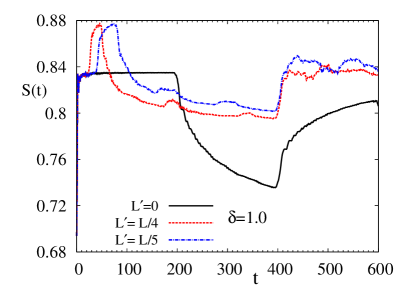
Figure 8: The plot shows EE as a function of time for single and double quenches when the whole chain is non-critical ($h=0.5$) with $L_{1}=100$, $L_{A}=100$ and $L=300$ and different $L^{\prime}$. For $L^{\prime}=L/4$, the deviation in EE from single quenching case starts at $t=t^{\prime}/2$ where $t^{\prime}=50$, with $v_{\max}=2h=1$. For $t>50$, both $QP^{2}_{L}$ and $QP^{2}_{R}$ are in system B leading to decrease in EE which continues up to $t_{4}=400$. Similarly, for $L^{\prime}=L/5$ one can find $t^{\prime}=80$ and the figure shows the expected behavior. The absence of $t^{\prime\prime}$ is explained in the text.

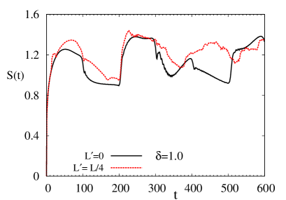
Figure 9: EE as a function of time for the same situation as in Fig8 but fixing $h$ at $0.99$. In this case the value of $v_{\max}$ is $1.98$. This gives $t^{\prime}=25.25$ for $L^{\prime}=L/4$. We do see timescales $t^{\prime}/2$ and $t^{\prime}$ along with $t_{3}$ ($\sim$ 101) and $t_{4}$ ($\sim$ 202). We also observe a peak near $t^{\prime\prime}$ ($\sim$ 227).

V Comparison between $QP^{1}$ and $QP^{2}$

In this section we try to argue why the effect of $QP^{2}$ is stronger than $QP^{1}$. As discussed before, the initial state, which is no longer the ground state of the final Hamiltonian, is a source of quasiparticles. Also, since the perturbation studied in this paper is local and very small, the quasiparticles are produced at the site of perturbation only, i.e., at $L^{\prime}$ and $L_{1}$. These quasiparticles have energies given by the eigenvalues of the final Hamiltonian. Let $k$ identifies the quasiparticle $\eta_{k}$ having eigen energy $\Lambda_{k}$. Quasiparticles of energy $\Lambda_{k}$ are produced at the perturbation site with probability $f_{k}$. Numerically, one can obtain $f_{k}$ by calculating the expectation value

$$f_{k}=\langle\psi_{i}|\eta_{k}^{\dagger}\eta_{k}|\psi_{i}\rangle$$

which is proportional to the number of quasiparticles $\eta_{k}$ present in the initial state $|\psi_{i}\rangle$. This expression can be written in terms of $\Phi_{k}$, $\Psi_{k}$ of the final Hamiltonian and the matrix $G^{i}$ (see Appendix B) with respect to the initial Hamiltonian. A comparison of $f_{k}$ for the h-quench alone ($h$ changed from $1$ to $2$ at $L^{\prime}$), $J$-quench alone (0 to 1 at $L_{1}$) and both quenches together is shown in Fig. 10. Clearly, quasiparticle creation probability is an order of magnitude higher in case of $J$-quench alone when compared to $h$-quench. This hints to the fact that the $J$-quench is the main source of quasiparticle production and hence our numerical results are dominated by the dynamics of $QP^{2}$.

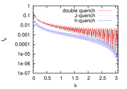
Figure 10: Variation of $f_{k}$ with $k$ for a critical chain. The dashed line or the lowest curve corresponds to the h-quench case which clearly is an order of magnitude smaller than the J-quench alone. Similar behavior is also observed for a ferromagnetic chain.

VI Conclusions and Discussions

In this paper, we studied the effect of two simultaneous local quenches in an otherwise uniform transverse Ising chain of length $L$ with open boundary conditions. Initially, the system is prepared in the ground state of the transverse Ising chain having a uniform transverse field $h$ and the interaction strength set to unity at all sites except $J_{L_{1}}$ and $J_{L}$ where it is zero. The first quench corresponds to sudden increase of $J_{L_{1}}$ from zero to $1$, and the second quench involves the sudden change of the transverse field from $h$ to $h+\delta$ at site $L^{\prime}$. We argued that the sites of the two local quenches are source of quasiparticle production as there is a local increase in energy due to the quenches. These QPs are wavepackets of low lying excitations of the final Hamiltonian. As discussed in Refs rieger11 ; blass12 , the QPs are localized in the ferromagnetic region and behave more like classical particles, whereas they are extended objects/wavepackets as the critical point is approached.

We numerically studied the evolution of Loschmidt echo and entanglement entropy after the double quenches and explained the evolution using the quasiparticle picture. The envelope of the curve is dictated by the fastest moving quasiparticles. We showed taking examples that most of the timescales can be explained using the propagation of quasiparticles. The most interesting phenomena that is observed numerically is the partial or full reflection of the quasiparticles at $L^{\prime}$, the site of $h-$quench. Only if we include such a phenomena that we can explain certain numerically observed time scales. As mentioned in details in the paper, the most relevant time scales are $t^{\prime}$, $t_{3}$, $t_{4}$ and $t^{\prime\prime}$ (for $L_{1}=L_{A}$) which are all due to the $QP^{2}$ pair, or the pair produced at the J-quenching site. The presence of the other set of quasiparticles, namely, $QP^{1}$ is clearly seen in the evolution of EE. We have shown that the probability of quasiparticles produced due to h-quench is roughly an order of magnitude smaller than the J-quench which could be the reason for stronger effect of $QP^{2}$ in the evolution of LE and EE.

The double quenches deep inside the ferromagnetic phase can be very nicely described by the point like quasiparticles where all the time scales are sharply observed. We have contrasted this ferromagnetic case with the double quenches in the critical phase and proposed the reasons for their differences. It seems that the reflection of $QP^{2}$ at $L^{\prime}$ in a critical chain is only partial having a transmitted component also. This can be attributed to extended wavepacket nature of quasiparticles at the critical point. One can then explain the decrease of EE at $t=t_{3}$, slight increase of EE for $t>t^{\prime}$ after the sharp decrease at $t^{\prime}$, and the dip at $t=T$.

Our main aim in this paper is to study the dynamical evolution of LE and EE after double quenches and see if one can explain the behavior, atleast qualitatively, using propagation of quasiparticles. We have demonstrated here that this indeed is possible. Though we can not propose a general formula for all the timescales involved as it depends on which quasiparticle arrives at the subsystem first, which in turn depends on the location of $L^{\prime}$, $L_{1}$ and $L_{A}$, but the basic idea gives us the right picture. We have checked this for other cases also which are not presented in this paper. The quasiparticle picture does explain many features, if not all, of the dynamical evolution of LE and EE that occur in double quenches studied here. We have provided some arguments for the immediate increase of EE after $t^{\prime}$ for a critical chain which is related to the extended nature of the QPs at the critical point.

Acknowledgements UD acknowledges funding from DST-INSPIRE Faculty fellowship (IFA12-PH-45) by DST, Govt. of India. AR and UD sincerely thank Amit Dutta for fruitful discussions and the hospitality of IIT Kanpur where some parts of this work were done. AR acknowledges Bikas K Chakrabarti for useful comments.

Appendix A Loschmidt echo for a general quadratic fermionic system

Here we shall discuss the method for evaluating the time evolution of LE in real space for a general quadratic fermionic system rossini07 . We rewrite the Hamiltonian in Eq. (5) in the following form

$$H=\frac{1}{2}{\bf C^{\dagger}\,\mathcal{H}\,C},$$ (13)

where ${\bf C^{\dagger}}=\left(c_{1}^{\dagger},\ldots c_{L}^{\dagger},\,c_{1},\ldots c_{L}\right)$ and ${\bf\mathcal{H}}=\sigma^{z}\otimes{\bf A}+i\sigma^{y}\otimes{\bf B}$.

The Loschmidt echo, defined in Eq. (1) can be evaluated in this case by the following relation levitov96 ; rossini07

$$\mathcal{L}(t)=|\langle\psi(0)|e^{-itH_{f}}|\psi(0)\rangle|=|\mathrm{det}(1-\bf{R}+\bf{R}e^{-i\bf{\mathcal{H}_{f}}t})|,$$ (14)

where $H_{f}$ is the final Hamiltonian after double quenches. $\bf{R}$ is the $2L\times 2L$ correlation matrix whose elements are two-point correlation functions of fermionic operators $R_{ij}=\langle\psi(0)|C_{i}^{\dagger}C_{j}|\psi(0)\rangle$, where $|\psi(0)\rangle$ is the ground state of the initial Hamiltonian $H_{i}$. Following some mathematical steps we can the matrix $\bf{R}$ in terms of $\bf{g}$ and $\bf{h}$ matrices (see discussion around Eq. 8)

$${\bf R}=\left(\begin{array}[]{cc}{\bf h^{i}}\;{\bf(h^{i})^{T}}&\quad{\bf h^{i}}\;{\bf(g^{i})^{T}}\\ {\bf g^{i}}\;{\bf(h^{i})^{T}}&\quad{\bf g^{i}}\;{\bf(g^{i})^{T}}\end{array}\right).$$ (15)

Here, the $\bf{g}^{i}$ and $\bf{h}^{i}$ matrices are calculated relative to the initial Hamiltonian $H_{i}$. For more details, see Ref. rossini07

Appendix B Time dependant entanglement entropy for a general quadratic fermionic system

We outline here steps for calculating the time evolution of EE after sudden quenches igloi00 ; igloi09 . As discussed in the text, our model is reduced in quadratic form using spinless fermions. Let us define two Clifford operators which are also related to the Majorana fermion operators $a_{2i-1}$ and $a_{2i}$ in the following way,

$$\mathcal{A}_{i}=c_{i}^{\dagger}+c_{i}=a_{2i-1}\hskip 5.69054pt\text{and}\hskip 5.69054pt\mathcal{B}_{i}=c_{i}^{\dagger}-c_{i}=ia_{2i}.$$ (16)

The operators $\mathcal{A}$ and $\mathcal{B}$ can be written in terms of the free-fermion operators $\eta_{k}$

$$\mathcal{A}_{i}=\sum_{k=1}^{L}\Phi_{k}(i)(\eta_{k}^{\dagger}+\eta_{k}),\hskip 5.69054pt\mathcal{B}_{i}=\sum_{k=1}^{L}\Psi_{k}(i)(\eta_{k}^{\dagger}-\eta_{k}).$$ (17)

The time evolution of these operators are obtained from the time dependence of fermionic operators, i.e., $\eta_{k}(t)=e^{-it\Lambda_{k}}\eta_{k}$, where $\eta_{k}$ and $\Lambda_{k}$ are quasiparticles and eigen energies corresponding to the final Hamiltonian $H_{f}$. This is given by

$$\mathcal{A}_{i}(t)=\sum_{j=1}^{L}\left[\langle\mathcal{A}_{i}\mathcal{A}_{j}\rangle_{t}\mathcal{A}_{j}+\langle\mathcal{A}_{i}\mathcal{B}_{j}\rangle_{t}\mathcal{B}_{j}\right],$$ (18)

$$\mathcal{B}_{i}(t)=\sum_{j=1}^{L}\left[\langle\mathcal{B}_{i}\mathcal{A}_{j}\rangle_{t}\mathcal{A}_{j}+\langle\mathcal{B}_{i}B_{j}\rangle_{t}\mathcal{B}_{j}\right],$$ (19)

where the time-dependent contractions are

$$\langle\mathcal{A}_{i}\mathcal{A}_{j}\rangle_{t} = \sum_{k=1}^{L}\cos(\Lambda_{k}t)\Phi_{k}(i)\Phi_{k}(j)\;,$$

$$\langle\mathcal{A}_{i}\mathcal{B}_{j}\rangle_{t} = \langle B_{j}A_{i}\rangle_{t}=i\sum_{k=1}^{L}\sin(\Lambda_{k}t)\Phi_{k}(i)\Psi_{k}(j)\;,$$

$$\langle\mathcal{B}_{i}\mathcal{B}_{j}\rangle_{t} = \sum_{k=1}^{L}\cos(\Lambda_{k}t)\Psi_{k}(i)\Psi_{k}(j)\;.$$ (20)

The total system is divided into two subsystems $A$ and $B$ of length $L_{A}$ and $L_{B}$ respectively. To evaluate EE between these two subsystems after the double quench, we have to calculate the reduced density matrix $\rho_{A}$ of the subsystem $A$. This can be reconstructed from the $2L_{A}\times 2L_{A}$ correlation matrix of the Majorana operators

$$\langle\psi_{i}|a_{m}(t)a_{n}(t)|\psi_{i}\rangle=\delta_{m,n}+\imath(\Gamma^{A})_{mn},$$ (21)

where $m,n=1,2,3,\cdots,2L_{A}$ and $|\psi_{i}\rangle$ is the initial ground state. The matrix $\Gamma^{A}$ is an antisymmetric matrix which can be brought into the block-diagonal form by an orthogonal matrix say, $V$. Therefore the eigenvalues of $\Gamma^{A}$ are purely imaginary of the form $\pm\nu_{l}$ with $l=1,2,\cdots,L_{A}$. This can be used to write the reduced density matrix as a direct product of $L_{A}$ uncorrelated modes $\rho_{A}=\otimes_{l=1}^{L_{A}}\varrho_{l}$, where each $\varrho_{l}$ has eigenvalues $(1\pm\nu_{l})/2$. Thus the bipartite EE for $\rho_{A}$ is the sum of entropies of $L_{A}$ uncorrelated modes given by

$$S_{L}(L_{A})=-\sum_{l=1}^{L_{A}}\left(\frac{1+\nu_{l}}{2}\log\frac{1+\nu_{l}}{2}+\frac{1-\nu_{l}}{2}\log\frac{1-\nu_{l}}{2}\right).$$ (22)

The time-dependent expectation values in Eq. (21) are calculated using Eq. (19) as

$$\langle a_{2l}(t)a_{2m}(t)\rangle=-\langle\mathcal{B}_{l}(t)\mathcal{B}_{m}(t)\rangle,$$ (23)

$$\langle a_{2l-1}(t)a_{2m-1}(t)\rangle=-\langle\mathcal{A}_{l}(t)\mathcal{A}_{m}(t)\rangle,$$ (24)

$$\langle a_{2l}(t)a_{2m-1}(t)\rangle=-i\langle\mathcal{B}_{l}(t)\mathcal{A}_{m}(t)\rangle,$$ (25)

$$\langle a_{2l-1}(t)a_{2m}(t)\rangle=-i\langle\mathcal{A}_{l}(t)\mathcal{B}_{m}(t)\rangle.$$ (26)

Thus we shall get the time-dependent correlation matrix $\Gamma^{A}$ and for each time we can obtain EE from Eq. (22). The elements of the matrix $\Gamma^{A}$ are given by

$$\Gamma^{A}_{2l-1,2m-1} = -\imath\sum_{k_{1},k_{2}}G^{i}_{k_{1}k_{2}}\langle\mathcal{A}_{l}\mathcal{B}_{k_{1}}\rangle_{t}\langle\mathcal{A}_{m}\mathcal{A}_{k_{2}}\rangle_{t}$$

$$+ \imath\sum_{k_{1},k_{2}}G^{i}_{k_{2}k_{1}}\langle\mathcal{A}_{l}\mathcal{A}_{k_{1}}\rangle_{t}\langle\mathcal{A}_{m}\mathcal{B}_{k_{2}}\rangle_{t}$$

$$\Gamma^{A}_{2l-1,2m} = \sum_{k_{1},k_{2}}G^{i}_{k_{2}k_{1}}\langle\mathcal{A}_{l}\mathcal{A}_{k_{1}}\rangle_{t}\langle\mathcal{B}_{m}\mathcal{B}_{k_{2}}\rangle_{t}$$

$$- \sum_{k_{1},k_{2}}G^{i}_{k_{1}k_{2}}\langle\mathcal{A}_{l}\mathcal{B}_{k_{1}}\rangle_{t}\langle\mathcal{B}_{m}\mathcal{A}_{k_{2}}\rangle_{t}$$

$$\Gamma^{A}_{2l,2m-1} = -\sum_{k_{1}k_{2}}G^{i}_{k_{1}k_{2}}\langle\mathcal{B}_{l}\mathcal{B}_{k_{1}}\rangle_{t}\langle\mathcal{A}_{m}\mathcal{A}_{k_{2}}\rangle_{t}$$

$$+ \sum_{k_{1},k_{2}}G^{i}_{k_{2}k_{1}}\langle\mathcal{B}_{l}\mathcal{A}_{k_{1}}\rangle_{t}\langle\mathcal{A}_{m}\mathcal{B}_{k_{2}}\rangle_{t}$$

$$\Gamma^{A}_{2l,2m} = -\imath\sum_{k_{1},k_{2}}G^{i}_{k_{2}k_{1}}\langle\mathcal{B}_{l}\mathcal{A}_{k_{1}}\rangle_{t}\langle\mathcal{B}_{m}\mathcal{B}_{k_{2}}\rangle_{t}$$ (27)

$$+ \imath\sum_{k_{1},k_{2}}G^{i}_{k_{1}k_{2}}\langle\mathcal{B}_{l}\mathcal{B}_{k_{1}}\rangle_{t}\langle\mathcal{B}_{m}\mathcal{A}_{k_{2}}\rangle_{t}.$$

where $G^{i}_{k_{1}k_{2}}=-\sum_{k}\Psi_{k}^{i}(k_{1})\Phi_{k}^{i}(k_{2})$ is the equilibrium correlation function which is calculated with the initial Hamiltonian $H_{i}$.

References

- (1)
- (2) S. Haroche, Phys. Today 51 36 (1998).
- (3) W. H. Zurek, Rev. Mod. Phys. 75 715 (2003).
- (4) E. Joos, H. D. Zeh, C. Keifer, D. Giulliani, J. Kupsch and I. -O. Statatescu, Decoherence and appearance of a classical world in a quantum theory (Springer Press, Berlin) (2003).
- (5) A. Dutta, G. Aeppli, B. K. Chakrabarti, U. Divakaran, T. Rosenbaum and D. Sen, Quantum Phase Transitions in Transverse Field Spin Models: From Statistical Physics to Quantum Information, Cambridge University Press, (2015).
- (6) P. Zanardi and N. Paunkovic, Phys. Rev. E 74, 031123 (2006).
- (7) S. J. Gu, Int. J. Mod. Phys. B 24, 4371 (2010).
- (8) V. Gritsev, and A. Polkovnikov, in Developments in Quantum Phase Transitions, edited by L. D. Carr (Taylor and Francis, Boca Raton) (2010).
- (9) H.T. Quan, Z. Song, X.F. Liu, P. Zanardi, and C.P. Sun, Phys.Rev.Lett. 96, 140604 (2006).
- (10) J. Zhang, F. M. Cucchietti, C. M. Chandrasekhar, M. Laforest, C. A. Ryan, M. Ditty, A. Hubbard, J. K. Gamble and R. Laflamme, Phys. Rev. A 79, 012305 (2009).
- (11) D. Rossini, T. Calarco, V. Giovannetti, S. Montangero, and R. Fazio, Phys. Rev. A 75, 032333 (2007).
- (12) S. Sharma, Victor Mukherjee, and Amit Dutta, Eur. Phys. J B 85, 143(2012).
- (13) V. Mukherjee, S. Sharma, and A. Dutta, Phys. Rev. B 86, 020301 (R) (2012).
- (14) T. Nag, U. Diavakaran, and A. Dutta, Phys. Rev. B 86, 020401 (R) (2012).
- (15) S. Sharma and A. Rajak, J. Stat. Mech., P08005 (2012).
- (16) A. Peres, Phys. Rev. A 30 , 4 (1984).
- (17) T. J. Osborne and M. A. Nielsen, Phys. Rev. A 66, 032110 (2002).
- (18) A. Osterloh, L. Amico, G. Falci and R. Fazio, Nature 416, 608 (2002).
- (19) G. Vidal. J. I. Lattore, E. Rico, and A. Kitaev, Phys. Rev. Lett. 90, 227902 (2003). J. I. Lattore, E. Rico, and G. Vidal, arXiv:quant-ph/0304098v4 (2004).
- (20) V. E. Korepin, Phys. Rev. Lett. 92, 096402 (2004).
- (21) P. Calabrese and J. Cardy, J. Stat. Mech., P06002 (2004).
- (22) G. Refael and J. E. Moore, Phys. Rev. Lett. 93, 260602 (2004).
- (23) F. Igloi and Y. -C. Lin, J. Stat. Mech., P06004 (2008).
- (24) H. F. Song, C. Flindt S. Rachel, I. Klich, and K. Hur Le, Phys. Rev. B 83, 161408 (R) (2010).
- (25) J. Dubail and J. -M. Stephan, J. Stat. Mech. L03002 (2011).
- (26) C. Holzhey, F. Larsen, and F. Wilczek, Nucl. Phys. B 424, 443 (1994).
- (27) L. Amico, R. Fazio, A. Osterloh, and V. Vedral, Rev. Mod. Phys. 80, 517 (2008).
- (28) P. Calabrese, J. Cardy, and B. Doyon (ed), J. Phys. A: Math. Theor. 42, 500301 (2009).
- (29) J. Eiser, M. Cramer, and M. B. Plenio, Rev. Mod. Phys. 82, 277 (2010).
- (30) N. Laflorencie, Phys. Rev. B 72, 140408 (R) (2005).
- (31) G. De Chiara, S. Montangero, P. calabrese, and R. Fazio, J. Stat. Mech., P03001 (2006).
- (32) G. Refael and J. E. Moore, Phys. Rev. B 76, 024419 (2007).
- (33) N. E. Bonesteel and K. Yang, Phys. Rev. Lett. 99, 140405 (2007).
- (34) F. Igloi, Y.-C. Lin, H. Rieger, and C. Monthus, Phys. Rev. B 76, 064421 (2007).
- (35) F. Igloi, R. Juhasz, and Z. Zimboras, Euro. Phys. Lett. 79, 37001 (2007).
- (36) P. Calabrese and J. Cardy, J. Stat. Mech., P04010 (2005).
- (37) V. Eisler and I. Peschel, J. Stat. Mech., P06005 (2007).
- (38) P. Calabrese and J. Cardy, J. Stat. Mech., P10004 (2007).
- (39) V. Eisler, D. Karevski, T. Platini, and I. Peschel, J. Stat. Mech., P01023 (2008).
- (40) F. Igloi, Z. Szatmari, and Y. -C. Lin, Phys. Rev. B 80, 024405 (2009).
- (41) B. Hsu, E. Grosfeld, and E. Fradkin, Phys. Rev. B 80, 235412 (2009).
- (42) J. Cardy, Phys. Rev. Lett. 106, 150404 (2011).
- (43) J.-M. Stephan and J. Dubail, J. Stat. Mech., P08019 (2011).
- (44) F. Igloi, Z. Szatmari, and Y.-C. Lin, Phys. Rev. B 85, 094417 (2012).
- (45) I. Bloch, J. Dalibard, and W. Zwerger, Rev. Mod. Phys. 80, 885 (2008).
- (46) E. Lieb and T. Schultz and D. Mattis, Ann. Phys.,NY 16, 37004 (1961).
- (47) P. Pfeuty, Ann. Phys. (NY) 57, 79 (1970).
- (48) F. Igloi and H. Rieger, Phys. Rev. Lett. 106, 035701 (2011) H. Rieger and F. Igloi, Phys. Rev. B 84, 165117 (2011).
- (49) B. Blass, H. Rieger and F. Igloi, Euro. Phys. Lett. 99, 30004 (2012).
- (50) U. Divakaran, F. Igloi and H. Rieger, J. Stat Mech 11, 10027 (2011).
- (51) L.S. Levitov, H. Lee, and G.B. Lesovik, J. Math. Phys. 37, 4845 (1996); I. Klich, in Quantum Noise in Mesoscopic Physics, Yu.V. Nazarov Ed., NATO Science Series, Vol. 97 (Kluwer Academic Press, 2003).
- (52) F. Igloi and H. Rieger, Phys. Rev. Lett. 85, 3233 (2000).