Variational Inference for Background Subtraction in Infrared Imagery

Abstract

We propose a Gaussian mixture model for background subtraction in infrared imagery. Following a Bayesian approach, our method automatically estimates the number of Gaussian components as well as their parameters, while simultaneously it avoids over/under fitting. The equations for estimating model parameters are analytically derived and thus our method does not require any sampling algorithm that is computationally and memory inefficient. The pixel density estimate is followed by an efficient and highly accurate updating mechanism, which permits our system to be automatically adapted to dynamically changing operation conditions. Experimental results and comparisons with other methods show that our method outperforms, in terms of precision and recall, while at the same time it keeps computational cost suitable for real-time applications.

1 Introduction

Pixels values of infrared frames correspond to the relative differences in the amount of thermal energy emitted or reflected from objects in the scene. Due to this fact, infrared cameras are equally applicable for both day and night scenarios, while at the same time, compared to visual-optical cameras, are less affected by changing illumination or background texture. Furthermore, infrared imagery eliminates any privacy issues as people being depicted in the scene can not be identified [13]. These features make infrared cameras prime candidate for persistent video surveillance systems.

Although, infrared imagery can alleviate several problems associated with visual-optical videos, it has its own unique challenges such as a) low signal-to-noise ratio (noisy data) and b) almost continuous pixel values that model objects’ temperature. Both issues complicate pixel responses modeling. An example of raw thermal responses is presented in Figure 1, where pixel values are floating point numbers ranging from 293 to 299 Kelvin degrees. Due to this peculiarity most of conventional computer vision techniques, that successfully used for visual-optical data, can not be applied straightforward on thermal imagery.

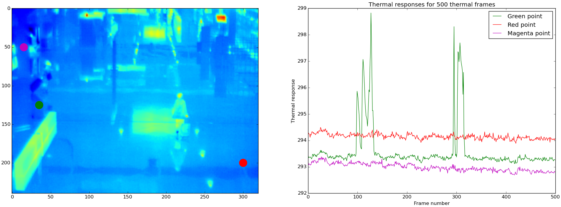
Fig. 1: Thermal responses for three different points. In contrast to visual-optical videos, where pixels take integer values, thermal responses are floating point numbers, corresponding to objects’ temperature.

For many high-level vision based applications, either they use visual-optical videos [4, 21, 24, 25] or infrared data [16, 17, 26], the task of background subtraction constitutes a key component, as this is one of the most common methods for locating moving objects, facilitating search space reduction and visual attention modeling.

Background subtraction techniques applied on visual-optical videos model the color properties of depicted objects [3, 15] and can be classified into three main categories [10]: basic background modeling [19, 28], statistical background modeling [11, 27] and background estimation [20, 23]. The most used methods are the statistical ones due to their robustness to critical situations. In order to statistically represent the background, a probability distribution is used to model the history of pixel values intensity over time. Towards this direction, the work of Stauffer and Grimson [22], is one of the best known approaches. It uses a Gaussian mixture model, with fixed number of components, for a per-pixel density estimate. Similar to this approach, Makantasis et al. in [18] propose a Student-t mixture model for background modeling, taking advantage of Student-t distribution compactness and robustness to noise and outliers. The works of [29] and [30] extend the method of [22] by introducing a rule based on a user defined threshold to estimate the number of components. However, this rule is application dependent and not directly derived from the data. Haines and Xiang in [14] address this drawback by using a Dirichlet process mixture model. Due to the computational cost of their method, the authors propose a GPU implementation. All of the aforementioned techniques present the drawback that objects’ color properties are highly affected by scene illumination, making the same object to look completely different under different lighting or weather conditions.

Although, thermal imagery can provide a challenging alternative for addressing the aforementioned difficulty, there exist few works for thermal data. The authors of [7, 8, 9] exploit contour saliency to extract foreground objects. Initially, they utilize a unimodal background modeling technique to detect regions of interest and then exploit the halo effect of thermal data for extracting foreground objects. However unimodal background modeling is not usually capable of capturing background dynamics. Baf et al. in [10] present a fuzzy statistical method for background subtraction to incorporate uncertainty into the mixture of Gaussians. However, this method requires a predefined number of components making this approach to be application dependent. Elguebaly and Bouguila in [12] propose a finite asymmetric generalized Gaussian mixture model for object detection. Again this method requires a predefined maximum number of components, presenting therefore limitations when this technique is applied on uncontrolled environments. Dai et al. in [5] propose a method for pedestrian detection and tracking using infrared imagery. This method consists of a background subtraction technique that exploits a two-layer representation (one for foreground and one for background) of infrared frame sequences. However, the assumption made is that the foreground is restricted to moving objects, a consideration which is not sufficient for dynamically changing environments. One way to handle the aforementioned difficulties is to introduce a background model, the parameters and the structure of which are directly estimated from the data, while at the same time it takes into account the specific properties of infrared imagery.

1.1 Our contribution

This work presents background modeling able to provide a per pixel density estimate, taking into account the special characteristics of infrared imagery, such as low signal-to-noise ratio. Our method exploits a Gaussian mixture model with unknown number of components. The advantage of such a model is that its own parameters and structure can be directly estimated from the data, allowing dynamic model adaptation to uncontrolled and changing environments.

An important issue in the proposed Gaussian mixture modeling concerns learning the model parameters. In our method, this is addressed using a variational inference framework to correspond the functional structure of the model with real data distributions obtained from the infrared images. Then, the Expectation-Maximization (EM) algorithm is adopted to fit the outcome of variational inference to real measurements. Updating procedures are incorporated to allow dynamic model adaptation to the forthcoming infrared data. Our updating method avoids of using heuristics by considering existing knowledge accumulated from previous data distributions and then it compensates this knowledge with current measurements.

Our overall strategy exploits a Bayesian framework to estimate all the parameters of the mixture model and thus avoiding over/under fitting issues. To compensate computational challenges arising from the non a priori known nature of the mixture model, we utilize conjugate priors and thus we derive analytical equations for model estimation. In this way, we avoid the need of any sampling method, which are computationally and memory inefficient. This selection makes our system suitable for online and real-time applications.

This paper is organized as follows: Section 2 formulates the Bayesian framework for mixture modeling. In Section 3 we present the procedure to analytically derive the solutions for estimating the distributions of model parameters. Section 4 describes the EM algorithm along with setting the priors and parameters initialization. Section 5 discusses the online updating mechanism and Section 6 presents the background subtraction task. In Section 7 experimental results are given and Section 8 concludes this work.

2 Gaussian mixture modeling

In this section we formulate the Bayesian framework adopted in this paper to analytically estimate all the parameters of the proposed Gaussian mixture model. For this reason, in section 2.1 we briefly describe the basic theory behind Gaussian mixture model, while in section 2.2 we describe the introduction of conjugate priors that assist us in yielding analytical model estimations as in Section 3.

2.1 Model fundamentals

The Gaussian mixture distribution can be seen as a linear superposition of Gaussian functional components,

$$p(x|\bm{\varpi},\bm{\mu},\bm{\tau})=\sum_{k=1}^{K}\varpi_{k}\mathcal{N}(x|\mu_{k},\tau_{k}^{-1})$$ (1)

where the parameters $\{\varpi_{k}\}_{k=1}^{K}$ must satisfy $0\leq\varpi_{k}\leq 1$ for every $k$ and $\sum_{k=1}^{K}\varpi_{k}=1$ and $K$ is the number of Gaussian components. In the proposed mixture modeling, variable $K$ can take any natural value up to infinity. However, it is highly recommended to set the upper bound for $K$ less than the cardinality of the dataset, i.e. the number of observed samples. By introducing a $K$-dimensional binary latent variable $\bm{z}$, such as $\sum_{k=1}^{K}z_{k}=1$ and $p(z_{k}=1)=\varpi_{k}$, the distribution $p(x)$ can be defined in terms of a marginal distribution $p(\bm{z})$ and a conditional distribution $p(x|\bm{z})$ as follows

$$p(x|\bm{\varpi},\bm{\mu},\bm{\tau})=\sum_{\bm{z}}p(\bm{z}|\bm{\varpi})p(x|\bm{z},\bm{\mu},\bm{\tau})$$ (2)

where $p(\bm{z}|\bm{\varpi})$ and and $p(x|\bm{z})$ are in the form of

$$p(\bm{z}|\bm{\varpi})=\prod_{k=1}^{K}\varpi_{k}^{z_{k}}$$ (3)

$$p(x|\bm{z},\bm{\mu},\bm{\tau})=\prod_{k=1}^{K}\mathcal{N}(x|\mu_{k},\tau_{k}^{-1})^{z_{k}}$$ (4)

where $\bm{\mu}=\{\mu_{k}\}_{k=1}^{K}$ and $\bm{\tau}=\{\tau_{k}\}_{k=1}^{K}$, correspond to the mean values and precisions of Gaussian components. By introducing latent variables and transforming the Gaussian mixture distribution into the form of (2), we are able to exploit the EM algorithm for fitting our model to the observed data, as shown in Section 4.

If we have in our disposal a set $\bm{X}=\{x_{1},...,x_{N}\}$ of observed data we will also have a set $\bm{Z}=\{\bm{z}_{1},...,\bm{z}_{N}\}$ of latent variables. Each $\bm{z}_{n}$ will be a $K$-dimensional binary vector, such as $\sum_{k=1}^{K}z_{nk}=1$, and, in order to take into consideration the whole dataset of $N$ samples, the distributions of (3) and (4) will be transformed to

$$p(\bm{Z}|\bm{\varpi})=\prod_{n=1}^{N}\prod_{k=1}^{K}\varpi_{k}^{z_{nk}}$$ (5)

$$p(\bm{X}|\bm{Z},\bm{\mu},\bm{\tau})=\prod_{n=1}^{N}\prod_{k=1}^{K}\mathcal{N}(x_{n}|\mu_{k},\tau_{k}^{-1})^{z_{nk}}$$ (6)

2.2 Conjugate priors

To avoid computational problems in estimating the parameters and the structure of the proposed Gaussian model, we introduce conjugate priors, over the model parameters $\bm{\mu}$, $\bm{\tau}$ and $\bm{\varpi}$, that allow us to yield analytical solutions. This way the need of using sampling methods is prevented. Introduction of priors implies the use of a Bayesian framework for the analysis.

Let us denote as $\bm{Y}=\{\bm{Z},\bm{\varpi},\bm{\mu},\bm{\tau}\}$ the set which contains all model latent variables and parameters and as $q(\bm{Y})$ its distribution. Then, our goal is to estimate $q(\bm{Y})$ which maximizes model evidence $p(\bm{X})$.

$$q(\bm{Y}):\max\ln p(\bm{X})$$ (7)

where in (7) we used the logarithm of $p(\bm{X})$ for calculus purposes. For maximizing (7) we need to define the distribution over $\bm{Y}$, that is, $p(\bm{Z}|\bm{\varpi})$ from (5), $p(\bm{\varpi})$ and $p(\bm{\mu},\bm{\tau})$.

Due to the fact that $p(\bm{Z}|\bm{\varpi})$ is a Multinomial distribution, its conjugate prior is a Dirichlet distribution over the mixing coefficients $\bm{\varpi}$

$$p(\bm{\varpi})=\frac{\Gamma(K\lambda_{0})}{\Gamma(\lambda_{0})^{K}}\prod_{k=1}^{K}\varpi_{k}^{\lambda_{0}-1}$$ (8)

where $\Gamma(\cdot)$ is the Gamma function. Parameter $\lambda_{0}$ has a physical interpretation; the smaller the value of this parameter is, the larger is the influence of the data rather than the prior on the posterior distribution $p(\bm{Z}|\bm{\varpi})$. In order to introduce uninformative priors and not prefer a specific component against the other, we choose to use a single parameter $\lambda_{0}$ for the Dirichlet distribution, instead of a vector with different values for each mixing coefficient.

Similarly, the conjugate prior of (4) takes the form of a Gaussian-Gamma distribution, because both $\bm{\mu}$ and $\bm{\tau}$ are unknown. Subsequently, the joint distribution of parameters $\bm{\mu}$ and $\bm{\tau}$ can be modeled as

$$p(\bm{\mu},\bm{\tau} )=p(\bm{\mu}|\bm{\tau})p(\bm{\tau})$$ (9a)

$$=\prod_{k=1}^{K}\mathcal{N}(\mu_{k}|m_{0},(\beta_{0}\tau_{k})^{-1})Gam(\tau_{k}|a_{0},b_{0})$$ (9b)

where $Gam(\cdot)$ denotes the Gamma distribution.

In order to not express any specific preference about the form of the Gaussian components through the introduction of priors, we use uninformative priors by setting the values of hyperparameters $m_{0}$, $\beta_{0}$, $a_{0}$ and $b_{0}$ to appropriate values as shown in Section 4.

Having defined the parametric form of observed data, latent variables and parameters distributions, our goal is to approximate the posterior distribution $p(\bm{Y}|\bm{X})$ and the model evidence $p(\bm{X})$, where $\bm{Y}=\{\bm{Z},\bm{\varpi},\bm{\mu},\bm{\tau}\}$ is the set with distribution $q(\bm{Y})$, which contains all model latent variables and parameters. Based on the Bayes rule, which states that $p(\bm{X})p(\bm{Y}|\bm{X})=p(\bm{X},\bm{Y})$ the logarithm of distribution $p(\bm{X})$ can be expressed as

$$\ln p(\bm{X}) =\int q(\bm{Y})\ln\frac{p(\bm{X},\bm{Y})}{q(\bm{Y})}d\bm{Y}-$$ (10a)

$$-\int q(\bm{Y})\ln\frac{p(\bm{Y}|\bm{X})}{q(\bm{Y})}d\bm{Y}$$

$$=\mathcal{L}(q)+KL(q||p)$$ (10b)

where $KL(q||p)$ is the Kullback-Leibler divergence between $q(\bm{Y})$ and $p(\bm{Y}|\bm{X})$ distributions and $\mathcal{L}(q)$ is the lower bound of $\ln p(\bm{X})$. Since $KL(q||p)$ is a non negative quantity, equals to zero only if $q(\bm{Y})$ is equal to $p(\bm{Y}|\bm{X})$, maximization of $\ln p(\bm{X})$ is equivalent to minimizing of $KL(q||p)$. For minimizing $KL(q||p)$ and estimating $p(\bm{X})$ we exploit the EM algorithm, as shown in Section 4.

By making the assumption, based on variational inference, that the distribution $q(\bm{Y})$ can be factorized over $M$ disjoint sets such as $q(\bm{Y})=\prod_{i=1}^{M}q_{i}(\bm{Y}_{i})$, as shown in [1], the optimal solution $q_{j}^{*}(Y_{j})$ corresponds to the minimization of $KL(q||p)$ is given by

$$\ln q_{j}^{*}(\bm{Y}_{j})=\mathbb{E}_{i\neq j}[\ln p(\bm{X},\bm{Y})]+\mathcal{C}$$ (11)

where $\mathbb{E}_{i\neq j}[\ln p(\bm{X},\bm{Y})]$ is the expectation of the joint distribution over all variables $\bm{Y}_{j}$ for $j\neq i$ and $\mathcal{C}$ is a constant. $P(\bm{X},\bm{Y})$ is modeled through (12).

In the following, we present the analytical solution for the optimal distributions $q_{j}^{*}(Y_{j})$ for model parameters and latent variables, i.e. the optimal distributions $q^{*}(\bm{Z})$, $q^{*}(\bm{\varpi})$, $q^{*}(\bm{\tau})$ and $q^{*}(\bm{\mu}|\bm{\tau})$.

3 Optimal model parameter distributions

According to (5), (6), (8) and (9), the joint distribution of all random variables can be factorized as follows

$$p(\bm{X},\bm{Z},\bm{\varpi},\bm{\mu},\bm{\tau})= p(\bm{X}|\bm{Z},\bm{\mu},\bm{\tau})p(\bm{Z}|\bm{\varpi})$$ (12)

$$p(\bm{\varpi})p(\bm{\mu}|\bm{\tau})p(\bm{\tau})$$

$\bm{X}$ corresponds to the set of the observed variables. All proofs are given in Appendix A.

3.1 Optimal $q^{*}(Z)$ distribution

Using (11) and the factorized form of (12) the distribution of the optimized factor $q^{*}(\bm{Z})$ is given by a Multinomial distribution of the form

$$q^{*}(\bm{Z})=\prod_{n=1}^{N}\prod_{k=1}^{K}\bigg{(}\frac{\rho_{nk}}{\sum_{j=1}^{K}\rho_{nj}}\bigg{)}^{z_{nk}}=$$ (13a)

$$\>\>\>\>\>\>\>\>\>\>\>\>=\prod_{n=1}^{N}\prod_{k=1}^{K}r_{nk}^{z_{nk}}$$ (13b)

as $\rho_{nk}$ we have denote the quantity

$$\rho_{nk}=\exp\bigg{(} \mathbb{E}\big{[}\ln\varpi_{k}\big{]}+\frac{1}{2}\mathbb{E}\big{[}\ln\tau_{k}\big{]}-\frac{1}{2}\ln 2\pi-$$ (14)

$$-\frac{1}{2}\mathbb{E}_{\bm{\mu},\bm{\tau}}\big{[}(x_{n}-\mu_{k})^{2}\tau_{k}\big{]}\bigg{)}$$

The expected value $\mathbb{E}[z_{nk}]$ of $q^{*}(\bm{Z})$ is equal to $r_{nk}$.

3.2 Optimal $q^{*}(\varpi)$ distribution

Using (12) and (11) the distribution of the optimized factor $q^{*}(\bm{\varpi})$ is given a Dirichlet distribution of the form

$$q^{*}(\bm{\varpi})=\frac{\Gamma(\sum_{i=1}^{K}\lambda_{i})}{\prod_{j=1}^{K}\Gamma(\lambda_{j})}\prod_{k=1}^{K}\varpi_{k}^{\lambda_{k}-1}$$ (15)

$\lambda_{k}$ is equal to $N_{k}+\lambda_{0}$, where $N_{k}=\sum_{n=1}^{N}r_{nk}$ represents the proportion of data that belong to the $k$-th component.

3.3 Optimal $q^{*}(\mu_{k}|\tau_{k})$ distribution

Similarly, the distribution of the optimized factor $q^{*}(\mu_{k},\tau_{k})$ is given by a Gaussian distribution of the form

$$q^{*}(\mu_{k}|\tau_{k})=\mathcal{N}(\mu_{k}|m_{k},(\beta_{k}\tau)^{-1})$$ (16)

where the parameters $m_{k}$ and $\beta_{k}$ are given by

$$\beta_{k} =\beta_{0}+N_{k}$$ (17a)

$$m_{k} =\frac{1}{\beta_{k}}\Big{(}\beta_{0}m_{0}+N_{k}\bar{x}_{k}\Big{)}$$ (17b)

where $\bar{x}_{k}$ is equal to $\frac{1}{N_{k}}\sum_{n=1}^{N}r_{nk}x_{n}$ represents the centroid of the data that belong to the $k$-th component.

3.4 Optimal $q^{*}(\tau_{k})$ distribution

After the estimation of $q^{*}(\mu_{k}|\tau_{k})$, distribution of the optimized factor $q^{*}(\tau_{k})$ is given by a Gamma distribution of the following form

$$q^{*}(\tau_{k})=Gam(\tau_{k}|a_{k},b_{k})$$ (18)

while the parameters $a_{k}$ and $b_{k}$ are given by the following relations

$$a_{k} =a_{0}+\frac{N_{k}}{2}$$ (19a)

$$b_{k} =b_{0}+\frac{1}{2}\bigg{(}N_{k}\sigma_{k}+\frac{\beta_{0}N_{k}}{\beta_{0}+N_{k}}\big{(}\bar{x}_{k}-m_{0}\big{)}^{2}\bigg{)}$$ (19b)

where $\sigma_{k}=\frac{1}{N_{k}}\sum_{n=1}^{N}(x_{n}-\bar{x}_{k})^{2}$.

4 Distribution parameters optimization

After the approximation of random variables distributions, we will use the EM algorithm in order to find optimal values for model parameters, i.e. maximize (10). In order to use the EM algorithm, we have to initialize priors hyperparameters $\lambda_{0}$, $a_{0}$, $b_{0}$, $m_{0}$ and $\beta_{0}$ and the model parameters $\varpi_{k}$, $\mu_{k}$, $\tau_{k}$, $\beta_{k}$, $a_{k}$, $b_{k}$ and $\lambda_{k}$ (see Section 3).

The parameter $\lambda_{0}$ can be interpreted as the effective prior number of observations associated with each component. In order to introduce an uninformative prior for $\bm{\varpi}$, we set the parameter $\lambda_{0}$ equal to $N/K$, suggesting that the same number of observations is associated to each component. Parameters $a_{0}$ and $b_{0}$ (positive values due to Gamma distribution) were set to the value of $10^{-3}$. Our choice is justified by the fact that the results of updating equations (19a) and (19b) are primarily affected by the data and not by the prior when the values for $a_{0}$ and $b_{0}$ are close to zero. The mean values of the components are described by conditional Normal distribution with means $m_{0}$ and precisions $\beta_{0}\tau_{k}$. We introduce an uninformative prior by setting the value for $m_{0}$ to the mean of the observed data and the parameter $\beta_{0}=\frac{b_{0}}{a_{0}v_{0}}$, where $v_{0}$ is the variance of the observed data.

The convergence of EM algorithm is facilitated by initializing the parameters $\varpi_{k}$, $\mu_{k}$, $\tau_{k}$ and $\beta_{k}$ using the k-means. To utilize k-means, the number of clusters, corresponding to the Gaussian components, should be a priori known. Since we create a mixture model, the number of Gaussian components should be less or equal to the number of observed data. For this reason we set the number of clusters $K_{max}$ to a value smaller or equal to the number of observations. If we have no clue about the number of classes we can set $K_{max}$ to equal $N$. If we denote as $\hat{N}_{k}$ the number of observation that belong to $k$-th cluster, then we can set the value of parameter $\mu_{k}$ to equal the centroid of $k$-th cluster, the parameter $\varpi_{k}$ to equal the proportion of observations for the $k$-th cluster, the parameter $\tau_{k}$ to equal $\hat{v}_{k}^{-1}$, where $v_{k}$ stands for the variance of the data of the $k$-th cluster and the parameter $\beta_{k}$ to equal $\hat{N}_{k}^{-1}$. Having initialized the parameters $\varpi_{k}$, $\mu_{k}$, $\tau_{k}$ and $\beta_{k}$, we can exploit the formula for the expected value of a Gamma distribution to initialize the parameters $a_{k}$ and $b_{k}$ to values $\tau_{k}$ and one respectively. Finally, the initialization of $\varpi_{k}$ allows us to initialize the parameter $\lambda_{k}$, which can be interpreted as the effective number of observations associated with each Gaussian component, to the value $N\varpi_{k}$.

After the initialization of model parameters and priors hyperparameters, the EM algorithm can be used to minimize $KL(q||p)$ of (10). During the E step, $r_{nk}$ is calculated given the initial/current values of all the parameters of the model. Using (13b) $r_{nk}$ is given by

$$r_{nk}\propto\tilde{\varpi_{k}}\tilde{\tau_{k}}^{1/2}\exp\bigg{(}-\frac{a_{k}}{2b_{k}}\big{(}x_{n}-m_{k}\big{)}^{2}-\frac{1}{2\beta_{k}}\bigg{)}$$ (20)

Due to the fact that $q^{*}(\bm{\varpi})$ is a Dirichlet distribution and $q^{*}(\tau_{k})$ is a Gamma distribution, $\tilde{\varpi_{k}}$ and $\tilde{\tau_{k}}$ will be given by

$$\ln\tilde{\varpi_{k}}\equiv\mathbb{E}\big{[}\ln\varpi_{k}\big{]}=\Psi(\lambda_{k})-\Psi\bigg{(}\sum_{k=1}^{K}\lambda_{k}\bigg{)}$$ (21a)

$$\ln\tilde{\tau_{k}}\equiv\mathbb{E}\big{[}\ln\tau_{k}\big{]}=\Psi(a_{k})-\ln b_{k}$$ (21b)

where $\Psi(\cdot)$ is the digamma function.

During the M step, we keep fixed the value for variables $r_{nk}$ (the value that was calculated during the E step), and we re-calculate the values for model parameters using (15), (17) and (19). The steps E and M are repeated sequentially untill the values for model parameters are not changing anymore. As shown in [2] convergence of EM algorithm is guaranteed because bound is convex with respect to each of the factors $q(\bm{Z})$, $q(\bm{\varpi})$, $q(\bm{\mu}|\bm{\tau})$ and $q(\bm{\tau})$.

During model training the mixing coefficient for some of the components takes value very close to zero. Components with mixing coefficient less than $1/N$ are removed (we require each component to model at least one observed sample) and thus after training the model has automatically determined the right number of Gaussian components.

5 Online updating mechanism

Having described how our model fits to $N$ observed data, in this section we present the mechanism that permits our model to automatically adapt to new observed data. We use no heuristic rules but statistics based on the observed data.

Let us denote as $x_{new}$ a new observed sample. Then, there are two cases; either the new observed sample is successfully modeled by our trained model, or not. To estimate if a new sample is successfully modeled, we find the closest component to the new sample. As a distance metric between components and the new sample, we use the Mahalanobis distance, since this is reliable distance measure between a point and a distribution.

The closest component $c$ to the new sample is the one that presents the minimum Mahalanobis distance $D_{k}$

$$c=\arg\min_{k}D_{k}=\arg\min_{k}\sqrt{(x_{new}-\mu_{k})^{2}\tau_{k}}$$ (22)

The probability of the new sample to belong to $c$

$$p(x_{new}|\mu_{c},\tau_{c})=\mathcal{N}(x_{new}|\mu_{c},\tau_{c}^{-1})$$ (23)

where $\mu_{c}$ and $\tau_{c}$ stand for the closest component mean value and precision respectively.

Let us denote as $\Omega$ the initially observed dataset. Then, we can assume that the probability to observe the new sample $x_{new}$ is given by

$$p(x_{new}|e)=\frac{N_{e}}{N}\mathcal{U}(x_{new}|x_{new}-e,x_{new}+e)$$ (24)

where $N_{e}=\big{|}\{x_{i}\in\Omega:x_{new}-e\leq x_{i}\leq x_{new}+e\}\big{|}$ and $\mathcal{U}(x_{new}|x_{new}-e,x_{new}+e)$ is a Uniform distribution with lower and upper bounds to equal $x_{new}-e$ and $x_{new}+e$ respectively. Equation (24) suggests that the probability to observe $x_{new}$ is related to the proportion of data that have already been observed around $x_{new}$. By increasing the neighborhood around $x_{new}$, i.e. increasing the value of $e$, the quantity $\mathcal{U}(x_{new}|x_{new}-e,x_{new}+e)$ is decreasing, while the value of $N_{e}$ is increasing.

Upon arrival of a new sample $x_{new}$, we can estimate the optimal range $\epsilon$ around $x_{new}$ that maximizes (24) as

$$\epsilon=\arg\max_{e}p(x_{new}|e)$$ (25)

Then, if $p(x_{new}|\mu_{c},\tau_{c})\geq p(x_{new}|\epsilon)$ the new observed sample $x_{new}$ can sufficiently represented by our model. Otherwise, a new Gaussian component must be created.

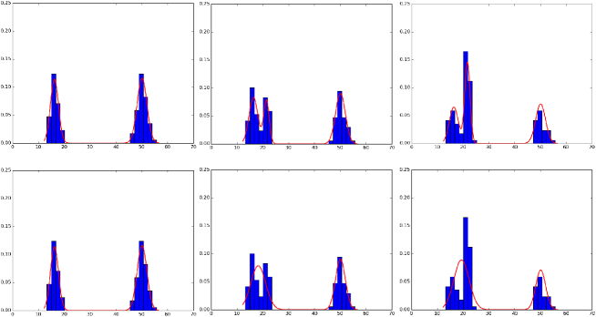
Fig. 2: First row: updating of our model to new observed data. Second row: updating of model presented in [29].

For model updating, we need to define the binary variable $o$, called ownership and associated with the Gaussian components, as

$$o_{k}=\begin{cases}1,&\mbox{if }k=c\\ 0,&\mbox{otherwise}\end{cases}$$ (26)

where we recall that $c$ represents the index of the closest component and $k$ is the index of $k$-th component.

When the new observed sample is successfully modeled, the parameters for the Gaussian components are updated using the following the leader [6] approach described as

$$\varpi_{k}\leftarrow\varpi_{k}+\frac{1}{N}\big{(}o_{k}-\varpi_{k}\big{)}$$ (27a)

$$\mu_{k}\leftarrow\mu_{k}+o_{k}\big{(}\frac{x_{new}-\mu_{k}}{\varpi_{k}N+1}\big{)}$$ (27b)

$$\sigma_{k}^{2}\leftarrow\sigma_{k}^{2}+o_{k}\bigg{(}\frac{\varpi_{k}N(x_{new}-\mu_{k})^{2}}{(\varpi_{k}N+1)^{2}}-\frac{\sigma_{k}^{2}}{\varpi_{k}N+1}\bigg{)}$$ (27c)

where $\sigma_{k}^{2}$ is equal to $\tau_{k}^{-1}$.

When the new observed sample cannot be modeled by the existing components, a new component is created with mixing coefficient $\varpi_{new}$, mean value $\mu_{new}$ and standard deviation $\sigma_{new}$, the parameters of which are given as

$$\varpi_{new}=\frac{1}{N}\>\>,\>\>\mu_{new}=x_{new}\>\>,\>\>\sigma_{new}^{2}=\frac{(2\epsilon)^{2}-1}{12}$$ (28)

From (28), we see that the mixing coefficient for the new component is equal to $1/N$ since it models only one sample (the new observed one), its mean value equals the value of the new sample and its variance the variance the Uniform distribution, whose the lower and upper bounds are $x_{new}-\epsilon$ and $x_{new}+\epsilon$ respectively. When a new component is created the values for the parameters for all the other components remain unchanged except mixing coefficients $\bm{\varpi}$, which are normalized to sum $\frac{N-1}{N}$. After each adaptation of the system to new observed samples, either they modeled by the trained model or not, the mixing coefficients of the components are normalized to sum to one.

Figure 2 presents the adaptation of our model (first row) and the model presented in [29] (second row) to new observed data. To evaluate the quality of the adaptation of the models, we used a toy dataset with 100 observations. Observed data were generated from two Normal distributions with mean values 16 and 50 and standard deviations 1.5 and 2.0 respectively. The initially trained models are presented in the left column. Then, we generated 25 new samples form a Normal distribution with mean value 21 and standard deviation 1.0. Our model creates a new component and successfully fits the data. On the contrary, the model of [29] is not able to capture the statistical relations of the new observations and fails to separate the data generated from distributions with mean values 16 and 21 (middle column). The quality of our adaptation mechanism becomes more clear in the right column, which presents the adaptation of both models after 50 new observations.

Algorithm 1: Overview of Background Subtraction

1:    capture $N$ frames

2:    create $N$-length history for each pixel

3:    initialize parameters (see Section 5)

4:    until convergence (training phase: Section 4)

5:          compute $r_{nk}$ using (20)

6:          recompute parameters using (15), (17) and (19)

7:    for each new captured frame

8:          classify each pixel as foreground or background

(see Section 6)

9:          update background model (see Section 5)

6 Background subtraction

In this section we utilize our model for background subtraction. We initially capture $N$ frames used to create an infrared responses history for each pixel. These histories act as observed data and used to train a model for each pixel. To classify a pixel of a new captured frame as background or foreground, we compute the probability its value to be represented by the mixture model. If this value is larger than a threshold the pixel is classified as background, otherwise it is classified as foreground. The threshold can be defined in relation to the parameters of the mixture, in order to be dynamically adapted. For example, we can define the threshold to be equal to $\mu_{c}\pm\nu\sigma_{c}$ where $\nu$ is a scalar defining a confidence interval. The overview of the background subtraction algorithm is shown in Algorithm 1.

7 Experimental results

For evaluating our algorithm, we used the Ohio State University (OSU) thermal datasets and a dataset captured at Athens International Airport (AIA) during Evacuate European funding project. OSU datasets contain frames that have been captured using a thermal camera and have been converted to grayscale images. In contrast, the AIA dataset contains raw thermal frames whose pixel values correspond to the real temperature of objects.

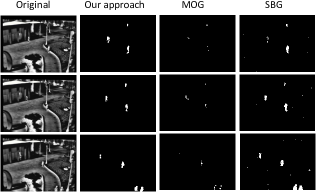
(a) OSU 1 dataset

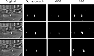
(a) OSU 2 dataset

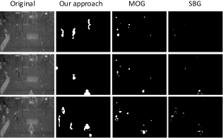
(a) AIA dataset

Fig. 3: Visual results for all datasets.

OSU datasets [7, 8, 9] are widely used for benchmarking algorithms for pedestrian detection and tracking in infrared imagery. Videos were captured under different illumination and weather conditions. AIA dataset was captured using a Flir A315 camera at different Airside Corridors and the Departure Level. Totally, 10 video sequences were captured, with frame dimensions $320\times 240$ pixels of total duration 32051 frames, at 7.5fps, that is, about 1h and 12mins. During experimentation process we used the sequence captured at the Departure Level Entrance 3 which provides a panoramic view of the space. The other sequences at corridors, due to narrow space perspective and the fact that videos were captured by mounting the camera at human height level, are inappropriate for testing background subtraction algorithms.

We compared our method with the method presented by Zivkovic in [29] (MOG), which is one of the most robust and widely used background subtraction technique, and with the method for extracting the regions of interest presented in [8, 9] (SBG) used for thermal data. To conduct the comparison we utilized the objective metrics of recall, precision and F1 score on a pixel wise manner. Figures 3 visually present the performance of the three methods. As is observed, our method outperforms both MOG and SBG on all datasets. While MOG and SBG perform satisfactory on grayscale frames of OSU datasets, their performance collapses when they applied on AIA dataset, which contains actual thermal responses. Regarding OSU datasets, MOG algorithm while presents high precision it yields very low recall values, i.e. the pixels that have been classified as foreground are indeed belong to the foreground class, but a lot of pixels that in fact belong to background have been misclassified. SBG algorithm seems to suffer by the opposite problem. Regarding AIA dataset, our method significantly outperforms both methods. In particular, while MOG and SBG algorithms present relative high precision, their recall values are under 0.2. Figure 4(a) presents average precision, recall and F1 score per dataset and per algorithm for all frames examined to give an objective evaluation. In Figure 4(b) presents the best and worst case in terms of precision, recall and F1 score among all frames examined.

Regarding computational cost, the main load of our algorithm is in the implementation of EM optimization. In all experiments conducted, the EM optimization converges within 10 iterations. Practically, the time required to apply our method is similar to the time requirements of Zivkovic’s method making it suitable for real-time applications.

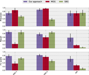
(a) Precision, recall and F1 score

(b) Best/worst case for precision, recall and F1 score

Fig. 4: Algorithms performance per dataset.

8 Conclusions

This paper presents a background subtraction method applicable to thermal imagery, based on Gaussian mixture modeling with unknown number. We analytically derive the solutions that describe the parameters of the model and we use the EM optimization to estimate their values, avoid sampling algorithms and high computational cost. Due to its low computational cost and the real-time operation, our method is suitable for real-world applications.

Appendix A Appendix

Using (11) and (12) the logarithm of $q^{*}(\bm{Z})$ is given by

$$\ln q^{*}(\bm{Z})= \mathbb{E}_{\bm{\varpi}}[\ln p(\bm{Z}|\bm{\varpi})]+$$ (29)

$$+\mathbb{E}_{\bm{\mu},\bm{\tau}}[\ln p(\bm{X}|\bm{Z},\bm{\mu},\bm{\tau})]+\mathcal{C}$$

substituting (5) and (6) into (29) we get

$$\ln q^{*}(\bm{Z})=\sum_{n=1}^{N}\sum_{k=1}^{K}z_{nk}\bigg{(}\mathbb{E}\big{[}\ln\varpi_{k}\big{]}+\frac{1}{2}\mathbb{E}\big{[}\ln\tau_{k}\big{]}-$$

$$\>\>\>\>\>\>\>\>\>\>-\frac{1}{2}\ln 2\pi-\frac{1}{2}\mathbb{E}_{\bm{\mu},\bm{\tau}}\big{[}(x_{n}-\mu_{k})^{2}\tau_{k}\big{]}\bigg{)}+\mathcal{C}\Rightarrow$$

Using (12) and (11) the logarithm of $q^{*}(\bm{\varpi},\bm{\mu},\bm{\tau})$ is

$$\ln q^{*}(\bm{\varpi},\bm{\mu},\bm{\tau}) =\mathbb{E}_{\bm{Z}}\big{[}\ln p(\bm{X}|\bm{Z},\bm{\mu},\bm{\tau})+$$

$$+\ln p(\bm{Z}|\bm{\varpi})+$$

$$+\ln p(\bm{\varpi})+\ln p(\bm{\mu},\bm{\tau})\big{]}+\mathcal{C}=$$ (31a)

$$=\sum_{n=1}^{N}\sum_{k=1}^{K}\mathbb{E}\big{[}z_{nk}\big{]}\ln\mathcal{N}(x_{n}|\mu_{k},\tau_{k}^{-1})+$$

$$+\mathbb{E}_{\bm{Z}}\big{[}\ln p(\bm{Z}|\bm{\varpi})\big{]}$$

$$+\ln p(\bm{\varpi})+\sum_{k=1}^{K}\ln p(\mu_{k},\tau_{k})+\mathcal{C}$$ (31b)

Due to the fact that there is no term in (31b) that contains parameters from both sets $\{\bm{\varpi}\}$ and $\{\bm{\mu},\bm{\tau}\}$, the distribution $q^{*}(\bm{\varpi},\bm{\mu},\bm{\tau})$ can be factorized as $q(\bm{\varpi},\bm{\mu},\bm{\tau})=q(\bm{\varpi})\prod_{k=1}^{K}q(\mu_{k},\tau_{k})$. The distribution for $q^{*}(\bm{\varpi})$ is derived using only those terms of (31b) that depend on the variable $\bm{\varpi}$. Therefore the logarithm of $q(\bm{\varpi})$ is given by

$$\ln q^{*}(\bm{\varpi}) =\mathbb{E}_{\bm{Z}}\big{[}\ln p(\bm{Z}|\bm{\varpi})\big{]}+\ln p(\bm{\varpi})+\mathcal{C}=$$ (32a)

$$=\sum_{k=1}^{K}\ln\varpi_{k}^{(\sum_{n=1}^{N}r_{nk}+\lambda_{0}-1)}+\mathcal{C}=$$ (32b)

$$=\sum_{k=1}^{K}\ln\varpi_{k}^{(N_{k}+\lambda_{0}-1)}+\mathcal{C}$$ (32c)

We have made use of $\mathbb{E}[z_{nk}]=r_{nk}$, and we have denote as $N_{k}=\sum_{n=1}^{N}r_{nk}$. (32c) suggests that $q^{*}(\bm{\varpi})$ is a Dirichlet distribution with hyperparameters $\bm{\lambda}=\{N_{k}+\lambda_{0}\}_{k=1}^{K}$.

Using only those terms of (31b) that depend on variables $\bm{\mu}$ and $\bm{\tau}$, the logarithm of $q^{*}(\mu_{k},\tau_{k})$ is given by

$$\ln q^{*}(\mu_{k},\tau_{k}) =\ln\mathcal{N}(\mu_{k}|m_{0},(\beta_{0}\tau_{k})^{1})+$$

$$\>\>\>\>\>+\ln Gam(\tau_{k}|a_{0},b_{0})+$$

$$\>\>\>\>\>+\sum_{n=1}^{N}\mathbb{E}\big{[}z_{nk}\big{]}\ln\mathcal{N}(x_{n}|\mu_{k},\tau_{k}^{-1})+\mathcal{C}=$$

$$=-\frac{\beta_{0}\tau_{k}}{2}(\mu_{k}-m_{0})^{2}+\frac{1}{2}\ln(\beta_{0}\tau_{k})+$$

$$\>\>\>\>\>+(a_{0}-1)\ln\tau_{k}-b_{0}\tau_{k}-$$

$$\>\>\>\>\>-\frac{1}{2}\sum_{n=1}^{N}\mathbb{E}\big{[}z_{nk}\big{]}(x_{n}-\mu_{k})^{2}\tau_{k}+$$

$$\>\>\>\>\>+\frac{1}{2}\bigg{(}\sum_{n=1}^{N}\mathbb{E}\big{[}z_{nk}\big{]}\bigg{)}\ln(\beta_{0}\tau_{k})+\mathcal{C}$$ (33)

For the estimation of $q^{*}(\mu_{k}|\tau_{k})$, we use (33) and keep only those factors that depend on $\mu_{k}$.

$$\ln q^{*}(\mu_{k}|\tau_{k}) =-\frac{\beta_{0}\tau_{k}}{2}\big{(}\mu_{k}-m_{0}\big{)}^{2}-$$

$$\>\>\>\>\>-\frac{1}{2}\sum_{n=1}^{N}\mathbb{E}\big{[}z_{nk}\big{]}\big{(}x_{n}-\mu_{k}\big{)}^{2}\tau_{k}=$$ (34a)

$$=-\frac{1}{2}\mu_{k}^{2}\Big{(}\beta_{0}+N_{k}\Big{)}\tau_{k}+$$

$$\>\>\>\>\>+\mu_{k}\tau_{k}\Big{(}\beta_{0}m_{0}+N_{k}\bar{x}_{k}\Big{)}+\mathcal{C}\Rightarrow$$ (34b)

$$q^{*}(\mu_{k}|\tau_{k})=\mathcal{N}(\mu_{k}|m_{k},(\beta_{k}\tau)^{-1})$$ (34c)

where $\bar{x}_{k}=\frac{1}{N_{k}}\sum_{n=1}^{N}r_{nk}x_{n}$, $\beta_{k}=\beta_{0}+N_{k}$ and $m_{k}=\frac{1}{\beta_{k}}(\beta_{0}m_{0}+N_{k}\bar{x}_{k})$.

After the estimation of $q^{*}(\mu_{k}|\tau_{k})$, logarithm of the optimized the distribution $q^{*}(\tau_{k})$ is given by

$$\ln q^{*}(\tau_{k}) =\ln q^{*}(\mu_{k},\tau_{k})-\ln q^{*}(\mu_{k}|\tau_{k})=$$ (35a)

$$=\bigg{(}a_{0}+\frac{N_{k}}{2}-1\bigg{)}\ln\tau_{k}-$$

$$\>\>\>\>\>\>-\frac{1}{2}\tau_{k}\bigg{(}\beta_{0}\big{(}\mu_{k}-m_{0}\big{)}^{2}+$$

$$\>\>\>\>\>\>+2b_{0}+\sum_{n=1}^{N}r_{nk}\big{(}x_{n}-\mu_{k}\big{)}^{2}-$$

$$\>\>\>\>\>\>-\beta_{k}\big{(}\mu_{k}-m_{k}\big{)}^{2}\bigg{)}+\mathcal{C}\Rightarrow$$ (35b)

$$q^{*}(\tau_{k})=Gam(\tau_{k}|a_{k},b_{k})$$ (35c)

The parameters $a_{k}$ and $b_{k}$ are given by

$$a_{k} =a_{0}+\frac{N_{k}}{2}$$ (36a)

$$b_{k} =b_{0}+\frac{1}{2}\bigg{(}N_{k}\sigma_{k}+\frac{\beta_{0}N_{k}}{\beta_{0}+N_{k}}\big{(}\bar{x}_{k}-m_{0}\big{)}^{2}\bigg{)}$$ (36b)

where $\sigma_{k}=\frac{1}{N_{k}}\sum_{n=1}^{N}(x_{n}-\bar{x}_{k})^{2}$.

References

- [1] C. Bishop. Pattern Recognition and Machine Learning (Information Science and Statistics). Springer, Oct. 2007.
- [2] S. Boyd and L. Vandenberghe. Convex Optimization. Cambridge University Press, Mar. 2004.
- [3] S. Brutzer, B. Hoferlin, and G. Heidemann. Evaluation of background subtraction techniques for video surveillance. In 2011 IEEE Conference on Computer Vision and Pattern Recognition (CVPR), pages 1937–1944, June 2011.
- [4] S.-C. S. Cheung and C. Kamath. Robust background subtraction with foreground validation for urban traffic video. EURASIP Journal on Advances in Signal Processing, 2005(14):726261, Aug. 2005.
- [5] C. Dai, Y. Zheng, and X. Li. Pedestrian detection and tracking in infrared imagery using shape and appearance. Computer Vision and Image Understanding, 106(2–3):288–299, May 2007.
- [6] S. Dasgupta and D. Hsu. On-line estimation with the multivariate gaussian distribution. In Proceedings of the 20th Annual Conference on Learning Theory, COLT’07, pages 278–292, Berlin, Heidelberg, 2007. Springer-Verlag.
- [7] J. Davis and V. Sharma. Fusion-based background-subtraction using contour saliency. In IEEE Computer Society Conference on Computer Vision and Pattern Recognition - Workshops, 2005. CVPR Workshops, pages 11–11, June 2005.
- [8] J. W. Davis and V. Sharma. Robust background-subtraction for person detection in thermal imagery. In Proceedings of the 2004 Conference on Computer Vision and Pattern Recognition Workshop (CVPRW’04) Volume 8 - Volume 08, CVPRW ’04, pages 128–, Washington, DC, USA, 2004. IEEE Computer Society.
- [9] J. W. Davis and V. Sharma. Background-subtraction in thermal imagery using contour saliency. International Journal of Computer Vision, 71(2):161–181, Feb. 2007.
- [10] F. El Baf, T. Bouwmans, and B. Vachon. Fuzzy statistical modeling of dynamic backgrounds for moving object detection in infrared videos. In IEEE Computer Society Conference on Computer Vision and Pattern Recognition Workshops, 2009. CVPR Workshops 2009, pages 60–65, June 2009.
- [11] A. Elgammal, D. Harwood, and L. Davis. Non-parametric model for background subtraction. In D. Vernon, editor, Computer Vision — ECCV 2000, number 1843 in Lecture Notes in Computer Science, pages 751–767. Springer Berlin Heidelberg, Jan. 2000.
- [12] T. Elguebaly and N. Bouguila. Finite asymmetric generalized gaussian mixture models learning for infrared object detection. Computer Vision and Image Understanding, 117(12):1659–1671, Dec. 2013.
- [13] R. Gade, A. Jorgensen, and T. Moeslund. Long-term occupancy analysis using graph-based optimisation in thermal imagery. In 2013 IEEE Conference on Computer Vision and Pattern Recognition (CVPR), pages 3698–3705, June 2013.
- [14] T. Haines and T. Xiang. Background subtraction with DirichletProcess mixture models. IEEE Transactions on Pattern Analysis and Machine Intelligence, 36(4):670–683, Apr. 2014.
- [15] S. Herrero and J. Bescós. Background subtraction techniques: Systematic evaluation and comparative analysis. In Proceedings of the 11th International Conference on Advanced Concepts for Intelligent Vision Systems, ACIVS ’09, pages 33–42, Berlin, Heidelberg, 2009. Springer-Verlag.
- [16] K. Jungling and M. Arens. Feature based person detection beyond the visible spectrum. In IEEE Computer Society Conference on Computer Vision and Pattern Recognition Workshops, 2009. CVPR Workshops 2009, pages 30–37, June 2009.
- [17] L. Latecki, R. Miezianko, and D. Pokrajac. Tracking motion objects in infrared videos. In IEEE Conference on Advanced Video and Signal Based Surveillance, 2005. AVSS 2005, pages 99–104, Sept. 2005.
- [18] K. Makantasis, A. Doulamis, and N. Matsatsinis. Student-t background modeling for persons’ fall detection through visual cues. In 2012 13th International Workshop on Image Analysis for Multimedia Interactive Services (WIAMIS), pages 1–4, May 2012.
- [19] N. J. B. McFarlane and C. P. Schofield. Segmentation and tracking of piglets in images. Machine Vision and Applications, 8(3):187–193, May 1995.
- [20] S. Messelodi, C. M. Modena, N. Segata, and M. Zanin. A kalman filter based background updating algorithm robust to sharp illumination changes. In F. Roli and S. Vitulano, editors, Image Analysis and Processing – ICIAP 2005, number 3617 in Lecture Notes in Computer Science, pages 163–170. Springer Berlin Heidelberg, Jan. 2005.
- [21] F. Porikli. Achieving real-time object detection and tracking under extreme conditions. Journal of Real-Time Image Processing, 1(1):33–40, Mar. 2006.
- [22] C. Stauffer and W. Grimson. Adaptive background mixture models for real-time tracking. In Computer Vision and Pattern Recognition, 1999. IEEE Computer Society Conference on., volume 2, pages –252 Vol. 2, 1999.
- [23] K. Toyama, J. Krumm, B. Brumitt, and B. Meyers. Wallflower: principles and practice of background maintenance. In The Proceedings of the Seventh IEEE International Conference on Computer Vision, 1999, volume 1, pages 255–261 vol.1, 1999.
- [24] O. Tuzel, F. Porikli, and P. Meer. Human detection via classification on riemannian manifolds. In IEEE Conference on Computer Vision and Pattern Recognition, 2007. CVPR ’07, pages 1–8, June 2007.
- [25] O. Tuzel, F. Porikli, and P. Meer. Pedestrian detection via classification on riemannian manifolds. IEEE Transactions on Pattern Analysis and Machine Intelligence, 30(10):1713–1727, Oct. 2008.
- [26] W. Wang, J. Zhang, and C. Shen. Improved human detection and classification in thermal images. In 2010 17th IEEE International Conference on Image Processing (ICIP), pages 2313–2316, Sept. 2010.
- [27] C. Wren, A. Azarbayejani, T. Darrell, and A. Pentland. Pfinder: real-time tracking of the human body. IEEE Transactions on Pattern Analysis and Machine Intelligence, 19(7):780–785, July 1997.
- [28] J. Zheng, Y. Wang, N. Nihan, and M. Hallenbeck. Extracting roadway background image: Mode-based approach. Transportation Research Record: Journal of the Transportation Research Board, 1944:82–88, Jan. 2006.
- [29] Z. Zivkovic. Improved adaptive gaussian mixture model for background subtraction. In Proceedings of the 17th International Conference on Pattern Recognition, 2004. ICPR 2004, volume 2, pages 28–31 Vol.2, Aug. 2004.
- [30] Z. Zivkovic and F. van der Heijden. Efficient adaptive density estimation per image pixel for the task of background subtraction. Pattern Recognition Letters, 27(7):773–780, May 2006.