Heliospheric Propagation of Coronal Mass Ejections:
Drag-Based Model Fitting

Abstract

The so-called drag-based model (DBM) simulates analytically the propagation of coronal mass ejections (CMEs) in interplanetary space and allows the prediction of their arrival times and impact speeds at any point in the heliosphere (“target”). The DBM is based on the assumption that beyond a distance of about 20 solar radii from the Sun, the dominant force acting on CMEs is the “aerodynamic” drag force. In the standard form of DBM, the user provisionally chooses values for the model input parameters, by which the kinematics of the CME over the entire Sun–“target” distance range is defined. The choice of model input parameters is usually based on several previously undertaken statistical studies. In other words, the model is used by ad hoc implementation of statistics-based values of the input parameters, which are not necessarily appropriate for the CME under study. Furthermore, such a procedure lacks quantitative information on how well the simulation reproduces the coronagraphically observed kinematics of the CME, and thus does not provide an estimate of the reliability of the arrival prediction. In this paper we advance the DBM by adopting it in a form that employs the CME observations over a given distance range to evaluate the most suitable model input parameters for a given CME by means of the least-squares fitting. Furthermore, the new version of the model automatically responds to any significant change of the conditions in the ambient medium (solar wind speed, density, CME–CME interactions, etc.) by changing the model input parameters according to changes in the CME kinematics. The advanced DBM is shaped in a form that can be readily employed in an operational system for real-time space-weather forecasting by promptly adjusting to a successively expanding observational dataset, thus providing a successively improving prediction of the CME arrival.

1 Introduction

Eruptive processes in the solar atmosphere, particularly coronal mass ejections (CMEs), strongly influence the physical state of the heliosphere and the terrestrial space environment. CMEs represent eruptive restructuring of the global coronal magnetic field, where the eruption itself is caused by a loss of equilibrium of the pre-eruptive magnetic field structure. The stability of the structure depends on the amount of energy stored in the magnetic field, whereas the CME itself is driven by the Lorentz force. The dynamics of the instability depends on the magnetic-flux conservation and inductive effects, which cause the cessation of the Lorentz force. Eventually, the magnetohydrodynamic (MHD) drag becomes a dominant factor in the CME dynamics. The drag is a consequence of collisionless transfer of momentum and energy between the CME and the ambient solar wind by MHD waves (Cargill, 2004).

In the present paper, we develop a method that provides the observations-driven adjustment of the input parameters of the so-called drag-based model (hereinafter, DBM), which describes the CME propagation in the interplanetary space by considering the “drag” force (for details see Vršnak et al. (2013), and references therein). The “drag” force depends on the relative speed of the ejection and the solar wind; in a collisionless environment the acceleration can be expressed as $a=-\gamma\left(v-w\right)\left|v-w\right|$, where $\gamma$ is the “drag parameter”, $a$ and $v$ refer to the instantaneous acceleration and speed of the ejection, whereas $w$ represents the ambient solar wind speed (Vršnak, 2001; Cargill, 2004; Owens & Cargill, 2004; Vršnak & Žic, 2007; Borgazzi et al., 2009; Lara & Borgazzi, 2009; Vršnak et al., 2010, 2013). Furthermore, the previously used DBM with constant $\gamma$ and $w$ parameters (Vršnak et al., 2013) is extended into a more general form, allowing variable $\gamma(r)$ and $w(r)$. In the DBM the CME is represented by the cone shape, where each element of the CME’s leading edge is defined by its position relative to the CME tip. The parameters $\gamma$ and $w$ represent the most sensitive elements of the DBM and play the main role in the drag-based simulation of heliospheric CME propagation. Consequently, their evaluation represents the central issue in DBM-based space-weather forecasting.

The paper is focused on the theoretical elaboration of finding values of the DBM parameters that give the smallest difference between the DBM-based kinematics and the CME kinematics as derived from observational data. The observational measurements could be derived from coronagraphic and heliospheric imaging data using several methods based on certain assumptions (e.g., fixed $\varphi$ for small CMEs: see Sheeley et al. 1999; Rouillard et al. 2008 or harmonic mean for large CMEs: see Lugaz et al. 2009). The presented fitting method opens the possibility of an “automatic” evaluation of the most appropriate DBM input parameters from observational data available for a particular event. The application and validation of the proposed method will be presented in a follow-up paper employing detailed coronal and heliospheric observations of one slow and one fast CME.

2 General description of the drag-based model

2.1 The drag force

In interplanetary space the CME motion is governed by the Lorentz force $F_{\mathrm{L}}$, gravity $F_{\mathrm{g}}$, and the MHD analog of the aerodynamic drag $F_{\mathrm{d}}$ (Vršnak, 2006). The net CME force can be expressed as:

$$F=F_{\mathrm{L}}-F_{\mathrm{g}}+F_{\mathrm{d}}.$$ (1)

At heliocentric distances beyond $R\gtrsim 15$, the MHD drag becomes a dominant force (Vršnak et al., 2009), so the CME motion is basically influenced solely by the $F_{\mathrm{d}}$ term of the force Equation (1).

Generally, the “drag” interaction between the solar wind and the CME in interplanetary space can be described in various ways. In this paper we consider the “drag” force of the form:

$$F_{\mathrm{d}}=-c_{\mathrm{d}}\,A\,\rho\,\left(v-w\right)\left|v-w\right|.$$ (2)

where $c_{\mathrm{d}}$ refers to the dimensionless drag coefficient, $A$ is the cross section of the CME, $\rho$ represents the ambient solar wind density, and $(v-w)$ is the velocity difference between the CME and the solar wind (Chen, 1989; Chen & Garren, 1993; Cargill et al., 1996, 2000; Cargill & Schmidt, 2002; Vršnak & Gopalswamy, 2002; Vršnak et al., 2004, 2009, 2010).

Following the numerical MHD simulations by Cargill (2004), and under the assumption that the CME structure does not change, we expect that the drag coefficient $c_{\mathrm{d}}$ varies slowly with radial distance and is approximately equal to 1 for the heliocentric distances beyond 15 solar radii, particularly in the case of dense CMEs. The mass density of a CME lies in the range of $12.7-13.5\,\mathrm{g}/r_{\odot}^{2}$, with the most dense events occurring during the solar maximum (see Vourlidas et al. (2011)). In this respect, we define dense CMEs as events with a mass density exceeding $13.2\,\mathrm{g}/r_{\odot}^{2}$.

The CME acceleration, caused by the MHD “drag” (Vršnak et al., 2009), can be written in a simple form using Equation (2):

$$a_{\mathrm{d}}=-\gamma\left(v-w\right)\left|v-w\right|,$$ (3)

where the parameter $\gamma$ is defined by

$$\gamma=c_{\mathrm{d}}\frac{A\rho}{M}.$$ (4)

The parameter $\gamma$ is inversely proportional to the total CME mass $M$, which consists of the initial mass and the so-called virtual mass that piles up as the CME expands in the inner heliosphere. Observations indicate that beyond heliocentric distances of several solar radii the total mass becomes approximately constant (Bein et al., 2013), implying that the mass pile-up becomes balanced by the mass loss (Vršnak & Žic, 2007; Vršnak et al., 2013).

2.2 Ambient density and solar wind speed

For the ambient density $\rho_{0}(r)=m_{\mathrm{p}}\,n_{0}(r)$, where $n_{0}(r)$ is unperturbed particle density and $m_{\mathrm{p}}$ is proton mass, the empirical $n_{0}(r)$ model proposed by Leblanc et al. (1998) is applied (referred to in the following as LDB, after Leblanc, Dulk, Bougeret). The CME cross section $A(r)$ depends on the geometrical shape of the CME; hereafter the cone representation is employed (Fisher & Munro, 1984; Xie et al., 2004; Schwenn et al., 2005). The parameter $\gamma(r)$ in Equation (3) defines the effectiveness of the drag force and depends on both the CME and the ambient solar wind.

At distances beyond $R\gtrsim 15$ ($R\equiv r/r_{\odot}$, where $r_{\odot}$ is the solar radius), the terms $\propto R^{-4}$ and $\propto R^{-6}$ in the LDB expression for $n_{0}(R)$ can be neglected. However, for the purposes of completeness and model development, in this paper the complete LDB density expression is applied:

$$n_{0}(R)=\frac{k_{2}}{R^{2}}+\frac{k_{4}}{R^{4}}+\frac{k_{6}}{R^{6}},$$ (5)

which is valid for radial distances $R>1.8$. Coefficients $k_{2}$, $k_{4}$ and $k_{6}$ read $k_{2}=3.3\times 10^{5}\,\mathrm{cm^{-3}}$, $k_{4}=4.1\times 10^{6}\,\mathrm{cm^{-3}}$ and $k_{6}=8.0\times 10^{7}\,\mathrm{cm^{-3}}$ (Leblanc et al., 1998).

The background solar wind is taken to be approximately stationary and isotropic, so from flux conservation, $\partial n_{0}/\partial t+\nabla\cdot(n_{0}\mathbf{w}_{0})=\mathbf{0}$, the solar wind speed must satisfy the expression:

$$w_{0}(R)=w_{\infty}\left(1+\frac{k_{4}/k_{2}}{R^{2}}+\frac{k_{6}/k_{2}}{R^{4}}\right)^{-1},$$ (6)

where $w_{\infty}$ is the asymptotic solar wind speed, i.e., $w_{\infty}=\lim_{R\rightarrow\infty}w_{0}(R)=const$. At small heliocentric distances the solar wind rarefies at a rate larger than $R^{-2}$, so the wind speed has to rise according to the continuity equation. Figure 1 shows the radial dependences of the normalized drag parameter $\gamma$, solar wind speed $w_{0}$ and density $n_{0}$. The presented ratios $\gamma(R)/\gamma_{\infty}$ and $w_{0}(R)/w_{\infty}$ are normalized by asymptotic values ($\gamma_{\infty}$ and $w_{\infty}$), and the ratio $n_{0}(R)/n_{\mathrm{1AU}}$ by the density value $n_{\mathrm{1AU}}$ at 1 AU. Note also that the value of $\gamma$ close to the Sun is for an order of magnitude larger than it is at large distances. As can be seen from Figure 1, one finds that the dependences $w_{0}(R)$, as well as $\gamma(R)$, become practically constant beyond $R\gtrsim 15$. Thus, the asymptotic values of $w_{0}$ and $\gamma$ are approximately equal to the values at 1 AU, i.e., $w_{\infty}\approx w_{\mathrm{1\,AU}}$ and $\gamma_{\infty}\approx\gamma_{\mathrm{1\,AU}}$. A similar simplification was used in previous papers (Vršnak & Žic, 2007; Vršnak et al., 2010, 2013) where the unperturbed solar wind speed and parameter-$\gamma$ functions had constant values, $w_{0}(R)=w_{\infty}$ and $\gamma(R)=\gamma_{\infty}$, for all radial distances.

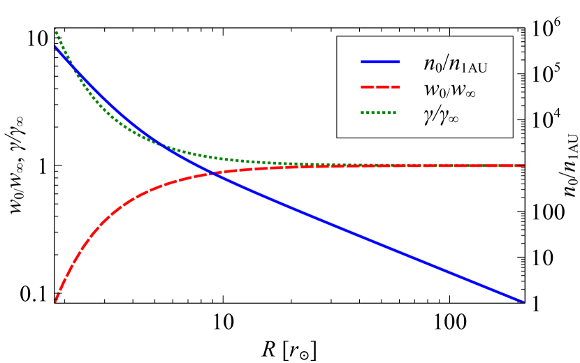
Figure 1: Radial dependence of the solar-wind density $n_{0}$ normalized by the density $n_{\mathrm{1AU}}$ at 1 AU ($n_{0}/n_{\mathrm{1AU}}$; solid line), shown together with the solar wind speed $w_{0}$ and the drag parameter ratio $\gamma$ normalized by their asymptotic values $w_{\infty}$ and $\gamma_{\infty}$ (dashed and dotted lines, respectively).

The solar wind speed $w_{0}(R)$ can be additionally modified by including a specific perturbation $w_{\mathrm{p}}(R)$ on top of the described undisturbed background to reproduce a particular situation in a given event. For example, in some cases the CME travels in interplanetary space through a region of locally enhanced or decreased solar-wind density (Temmer et al., 2011, 2012; Maričić et al., 2014; Rollett et al., 2014). In such a case the additional $w_{\mathrm{p}}(R)$ term should describe the associated solar wind speed perturbation in the region between the heliocentric distances $R_{1}$ and $R_{2}$. Under these assumptions, the perturbed solar wind speed is defined as

$$w(R)=\left\{\begin{array}[]{cc}w_{0}(R)+w_{\mathrm{p}}(R),&R_{1}<R<R_{2}\\ w_{0}(R),&\mathrm{otherwise}\end{array}\right.$$ (7)

where $w_{0}(R)$ represents the unperturbed solar wind speed (see Equation (6)). The perturbed density induced by the solar wind term $w_{\mathrm{p}}$ in $w(R)$,

$$n(R)=\frac{k_{2}}{R^{2}}\frac{w_{\infty}}{w(R)},$$ (8)

follows from flux conservation, i.e., $n(R)=\lim_{R_{\infty}\rightarrow\infty}[n_{0}(R_{\infty})\,R_{\infty}^{2}\,w_{0}(R_{\infty})/w(R)\,R^{2}]$. The perturbation is assumed to be localized over a finite region (i.e., inside the interval $R_{1}<R<R_{2}$), whereas the unperturbed expressions for the density, Equation (5), and solar wind speed, Equation (6), are valid otherwise.

The solar wind perturbation above is described by defining the wind speed $w_{\mathrm{p}}(R)$ from which follows the density profile $n(R)$; however, if the case study requires, the perturbation could be performed in the opposite way, firstly defining the density perturbation $n_{\mathrm{p}}(R)$ and afterward evaluating the solar wind speed expression $w(R)$.

2.3 Drag parameter $\gamma$

In the case of the CME propagation where the “drag” force is dominant, the equation of motion, Equation (3), transforms to

$$\ddot{R}(t)=-\gamma(R)\left[\dot{R}(t)-w(R)\right]\left|\dot{R}(t)-w(R)\right|.$$ (9)

The expression for $\gamma$ given by Equation (4) shows that the drag is more effective if the ambient density is high, if the CME is light, and if the CME cross section is large. In the present version of the DBM the effective CME cross section is defined by employing the CME “cone model” (Fisher & Munro, 1984; Xie et al., 2004; Schwenn et al., 2005). In this presentation, the cross-sectional area is given by $A=\pi\,r_{\odot}^{2}\,R^{2}\,\tan^{2}\lambda/(1+\tan\lambda)^{2}$, where $\lambda$ is the CME half-width (see the Appendix). Note that CMEs could be represented by a variety of geometrical representations; for examples of commonly used geometries see Schwenn et al. (2005), Thernisien et al. (2006), Lugaz et al. (2010), Thernisien (2011), Davies et al. (2012), and the references therein. Note that in the previous form of DBM with constant $w$ and $\gamma$ (Vršnak & Žic, 2007; Vršnak et al., 2010, 2013) the area was approximated by $A\approx\pi\,r_{\odot}^{2}\,R^{2}\,\lambda^{2}$. However, this did not have a direct influence on the calculated CME kinematics, since the value of $A$ was already incorporated within the presumed parameter $\gamma$.

Taking into account the definition of solar wind speed, Equation (7), $\gamma$ includes even the cases of perturbed solar wind, i.e., when the term $w_{\mathrm{p}}(R)$ is taken into account:

$$\gamma(R)=\gamma{}_{\infty}\frac{w_{\infty}}{w(R)}.$$ (10)

Since the asymptotic value of the solar wind speed at large heliocentric distances ($R\rightarrow\infty$) is $w_{\infty}$ (see Figure 1), evidently $\gamma(R)$ asymptotically acquires value $\gamma_{\infty}$ likewise, i.e., $\gamma_{\infty}=\lim_{R\rightarrow\infty}\gamma(R)$. In space-weather forecasting it became a practice to use a dimensionless variant $\Gamma$, defined by $\gamma_{\infty}=\Gamma\times 10^{-7}\,\mathrm{km^{-1}}$.

An interesting consequence follows from the dependence of the parameter $\Gamma$ on the CME’s geometrical shape and its properties. In the case when the effective cross section $A$ is proportional to the distance squared, $A\propto R^{2}$, $\Gamma$ could be generally calculated using $\Gamma=f(\lambda)/M$. The expression $f(\lambda)$ depends on the CME geometrical shape of the CME used in the model, which in our case is given by $f(\lambda)=\pi m_{p}r_{\odot}^{2}\,k_{2}\,\left[\tan\lambda/\left(1+\tan\lambda\right)\right]^{2}\times 10^{7}\,\mathrm{km}=8.4\times 10^{12}\,\left[\tan\lambda/\left(1+\tan\lambda\right)\right]^{2}\,\mathrm{kg}$ (see the Appendix). If the observations provide the CME half-width angle $\lambda$, and observed kinematics provide the value of $\Gamma$, the CME mass $M$ can be roughly estimated by employing $M=8.4\times 10^{12}\,\left[\tan\lambda/\left(1+\tan\lambda\right)\right]^{2}\,\Gamma^{-1}\,\mathrm{kg}$, where $\lambda$ is expressed in radians and $M$ in kg. The same holds for the opposite situation: knowing the mass $M$ one can estimate the angular half-width $\lambda$ from the value of $\Gamma$. The presumed geometrical shape of the CME affects the estimation of cross-sectional area, and consequently is important in evaluation of the unknown properties ($M$ or $\lambda$) of the CME. Thus, the best suited choice of the geometrical model to the CME observational properties improves the accuracy of the CME mass or half-width evaluation.

3 Model/observations fitting

In the following, the procedure of finding the values of any unknown DBM parameters is described. The drag parameter $\Gamma$, the background solar wind speed $w_{\infty}$, and the modified initial CME radial distance $R_{0}$ and speed $v_{0}$ are adjusted iteratively by minimizing the deviation of the model kinematics from the observed one. The process sequentially alters the DBM parameters in order to minimize the quadratic deviation (the sum of squared “errors” or residuals) between observational and DBM-calculated speeds:

$$E(\Gamma,w_{\infty};R_{0},v_{0})=\sum_{i=0}^{N}\left[v_{i}-v(\{\Gamma,w_{\infty};R_{0},v_{0}\},R_{i})\right]^{2}.$$ (11)

The observational distance–speed values are written as $R_{i}$ and $v_{i}$, while the adjusted kinematic curve $v(R)$, dependent on the model input parameters $\Gamma$, $w_{\infty}$ and the initial-state parameters $R_{0}$, $v_{0}$, is designated as $v(\{\Gamma,w_{\infty};R_{0},v_{0}\},R)$. The initial-state parameters depend on the presumed geometrical representation of a CME; therefore for the geometrical option presented in the Appendix, the initial-state parameters $R_{0}$ and $v_{0}$ of Equation (11) can have the CME tip values $R_{0}(t_{0})$, $v_{0}(t_{0})$, or the flank values $R_{\varphi}(t_{0})$, $v_{\varphi}(t_{0})$ at the initial time $t_{0}$, depending on the observer’s location (see the Appendix). Unknown input parameters are found by successively solving the equation of motion, Equation (9), within the parameter domain. In practice we use a more appropriate form of Equation (9), which reads

$$v(R)\,\frac{\mathrm{d}v(R)}{\mathrm{d}R}=-\gamma(R)\left[v(R)-w(R)\right]\left|v(R)-w(R)\right|.$$ (12)

The variation of the DBM parameters seeks the minimal value $E_{\mathrm{min}}$ of Equation (11). The presented method is basically a modified successive multiparametric variation that includes solving of the differential equation of motion, Equation (12), and least-squares fitting (hereafter, LSF) to the observational $\{(R_{0},v_{0}),\ldots,(R_{N},v_{N})\}$ dataset. Different approaches could be used in the numerical fitting. For example, the computation could be performed by starting with arbitrary DBM values based on which optimal values are found, or by numerically seeking the minimum of Equation (11) within a physically meaningful DBM-parameter domain (Motulsky & Ransnas, 1987). The meaningful parameter-domain restriction could be also included in the firstly mentioned approach to speed up the process of finding the $E_{\mathrm{min}}$. In the end, the minimal quadratic deviation gives the best input-parameter set $\{\Gamma,w_{\infty};R_{0},v_{0}\}$ for the specific observational event. Furthermore, kinematic curves, such as $a(R)$, $a(t)$, $v(R)$, $v(t)$, and $R(t)$ are automatically available from the calculated parameters. Consequently, this directly provides the CME transit time $\tau$, defined as the time the CME takes to arrive at a prescribed location, as well as the “impact” velocity $v_{\tau}$.

It is instructive to employ statistical analysis and to express the “goodness” of fit in the form of several statistical quantities. The first is the standard deviation (or the rms), which represents the average deviation between observed $v_{i}$ and calculated $v(R_{i})$ data:

$$\sigma=\sqrt{\frac{\sum_{i=0}^{N}\left[v_{i}-v(R_{i})\right]^{2}}{N+1}},$$ (13)

and gives data dispersion in velocity units (i.e. $\mathrm{km\,s^{-1}}$). Notice that the $(N+1)$ is the total number of observational datapoint samples $\{(R_{0},v_{0}),\ldots,(R_{N},v_{N})\}$.

The “goodness” could be graphically presented in the form of a residual plot. A residual plot shows the differences (or residuals) between each measured $v_{i}$ value and the value calculated from the estimated curve $v(R_{i})$, i.e., $[v_{i}-v(R_{i})]$. The residuals should not have a systematic dependence on $R$ values (the abscissa values) and should have a random scattering. Any clustering of residuals in the plot indicates that the prediction curve follows a systematic-error pattern and that the fit is not appropriate.

The next relevant criterion of scattering between observed values $v_{i}(R_{i})$ and calculated $v(R)$ is the coefficient of variation, which is defined by

$$c_{v}=\frac{\sigma}{\bar{v}}\cdot 100\%,$$ (14)

where $\bar{v}=\sum_{i=0}^{N}v(R_{i})/(N+1)$ is the mean of calculated values from the calculated set $\{v(R_{i})\}$.

Lastly, the coefficient of determination is defined by

$$\mathcal{R}^{2}=1-\frac{\sum_{i=0}^{N}\left[v_{i}-v(R_{i})\right]^{2}}{\sum_{i=0}^{N}\left[v_{i}-\bar{v}\right]^{2}},\quad 0\leq\mathcal{R}^{2}\leq 1$$ (15)

The “quality” of the estimated DBM parameters increases, i.e., the calculated kinematic curve fits observational data better, as $\sigma$ and $c_{\mathrm{v}}$ decrease and reach minimal values $\sigma_{\mathrm{min}}$ and $c_{\mathrm{vmin}}$, respectively. On the other hand, $\mathcal{R}^{2}$ becomes close to 1 as fit gets better (Motulsky & Ransnas, 1987).

For demonstration purposes we have chosen the observational dataset of Event 1 described in Temmer et al. (2011) and we have applied the LSF–DBM method to simulate the CME propagation. The event started on 2008 June 1 at $\sim 21\,\mathrm{UT}$ and the propagation data $\{R_{i},v_{i}\}$ with associated errors are derived from STEREO coronagraphic and heliospheric image data using the constrained harmonic mean method (see Rollett et al. 2012). For more details we refer to Temmer et al. (2011). The final result of the DBM fitting is presented in Figure 2, where panel 2(a) presents the velocity–distance profile of the calculated CME kinematics (blue solid line and accompanying shaded error area), as well as the estimated solar wind speed (green dashed line), together with the observational dataset (black circles) and its error bars. In the bottom panel (2(b)) we present the residulas, i.e., the relative difference $[v_{i}-v(R_{i})]/v_{i}$ between observational, $v_{i}$, and calculated, $v(R_{i})$, CME velocities, relative to the velocity $v_{i}$. The standard deviation of the observed dataset is $\sigma_{\mathrm{o}}=\sqrt{\sum_{i=0}^{N}e_{i}^{2}/(N+1)}=42.81\,\mathrm{km\,s^{-1}}$, where $e_{i}$ represents the half-error bar value for each measurement of velocity $v_{i}$. The LSF–DBM technique produced the fit with the DBM parameters $\Gamma=2.84$, $w_{\infty}=433.04\,\mathrm{km\,s^{-1}}$, $v_{0}=229.50\,\mathrm{km\,s^{-1}}$, $R_{0}=14.17\,r_{\odot}$, accompanied by the minimal standard deviation and the coefficients of variation and determination, $\sigma_{\mathrm{min}}=29.87\,\mathrm{km\,s^{-1}}$, $c_{\mathrm{vmin}}=7.50\,\%$, $\mathcal{R}^{2}=0.67$, respectively. In Figure 2(a) the “average” errors of the fit, spanning values frim $v(R)-\sigma_{\mathrm{min}}$ to $v(R)+\sigma_{\mathrm{min}}$, are drawn as the blue shaded area in the vicinity of the DBM kinematic curve $v(R)$. Evidently, the fitted standard deviation $\sigma_{\mathrm{min}}$ is much smaller than the observed $\sigma_{\mathrm{o}}$, showing that the LSF–DBM produced a satisfactory fit within the range of the “average observational error” $\sigma_{\mathrm{o}}$.

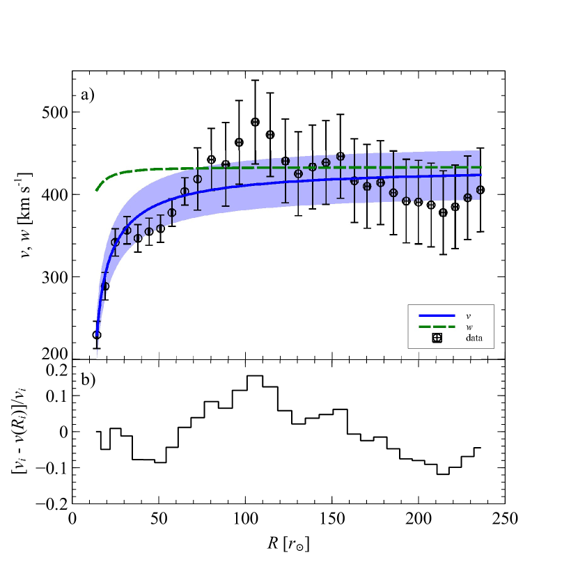
Figure 2: Application of the LSF–DBM method on the dataset extracted from Event 1 of the paper by Temmer et al. (2011). (a) Radial dependence of the LSF–DBM estimated kinematic curve $v(R)$ (solid blue line with error shown as the blue shaded area) on the observed CME speed values (black circles, with error bars), and numerically calculated solar wind speed $w$ (dashed green) based on parameter fitting. (b) Radial dependance of residuals, $v_{i}-v(R_{i})$, between observational $v_{i}$ and DBM-calculated $v(R_{i})$ speeds of CME (relative to observed CME speed $v_{i}$).

4 Discussion and conclusion

We have presented an extension of the DBM that is intended for use in automatic forecasting of CME arrival and impact at an arbitrary heliospheric position. The extension consists of optimizing the DBM input parameters based on the sequential variation and determination of the minimal standard deviation ($\sigma_{\mathrm{min}}$), the minimal coefficient of variation ($c_{\mathrm{vmin}}$), and the coefficient of determination ($\mathcal{R}^{2}$) from observational data. The mentioned statistical quantities represent an estimate of “goodness” of the DBM fit to observational data and consequently define the reliability of the arrival time and impact speed prediction. The presented LSF–DBM modification opens an opportunity for implementation in real-time space-weather forecasting tools and alerting systems for CME impacts on Earth (or any heliospheric “target” of interest). The novel approach is based on real-time data-driven DBM-parameter optimization that iteratively improves the accuracy of CME kinematics in the heliosphere.

The accuracy of the real-time forecasting increases as the observational dataset successively becomes larger, i.e., as the CME is tracked to larger heliospheric distances (Davis et al., 2010). For example, we can imagine a hypothetical case study of a CME launched from a region close to the solar disc center at a specific time $t=0$. In this case the CME is directed toward Earth and we can extract information about a current in situ solar wind speed $w_{\infty}$ at the Earth. On the other hand, the CME is traced in real time during its propagation throughout the heliosphere, so by using the most likely CME geometry the observational data can be transformed to get the distance–speed $(R_{i},v_{i})$ data. Every time when a new $(R_{i},v_{i})$ datapoint become available, the LSF procedure estimates a new set of DBM parameters required for updating the DBM forecast of CME arrival. As the dataset expands, our “impact prediction” becomes more reliable. In this respect it should be noted that an L5 mission is urgently needed to advance the performance of such forecasting methods. We note that this example is a quite simplified case in which the LSF–DBM method could be used.

There are several drawbacks of the described procedure, e.g., the estimation of the model input parameter and the related forecasting are highly dependent on the quality of the observational dataset. The input required for the DBM fitting procedure is the observed set of values for speed and distance of the CME frontal part as observed along the ecliptic plane. Several methods exist to derive those quantities, and we just mention briefly some possibilities. The propagation direction might be simply estimated from the CME associated source region, assuming radial propagation. In fact, knowing the propagation direction would enable one to derive the 3D CME kinematics from single spacecraft observations, such as, e.g., from STEREO heliospheric image data assuming a certain CME width (e.g., fixed $\phi$ for small CMEs: see Sheeley et al. 1999; Rouillard et al. 2008, or harmonic mean for large CMEs: see Lugaz et al. 2009). Using stereoscopic data, triangulation methods could be used that also provide the required input (coronagraphic field of view: see Mierla et al. 2010; interplanetary space: see Liu et al. 2010). The uncertainty of measurements is automatically forwarded to the estimated model parameters, and consequently, to the arrival time prediction.

Another serious drawback lies in the fact that the employed observational data include the distance range where the CME is still driven by the Lorentz force (Gallagher et al., 2003). In such a situation, the DBM fails in its fundamental concept because the Lorentz force is excluded from the modeling, i.e., only the drag force governs the CME propagation. However, it should be noted that even in such a case, the DBM kinematical curve might fit the observational data nicely due to the fact that the statistical weight dominantly comes from larger heliospheric distances, where the Lorentz force should be negligible. For example, if the observational dataset used in the modeling consists of only a few low-height measurements and a more abundant subset of measurements at larger heliocentric distances, the larger drag-dominated dataset “overweights” the smaller Lorentz-driven subset, so the latter effect becomes negligible.

The LSF and the DBM could be used in an opposite way to that previously discussed, for example to estimate the solar wind speed $w_{\infty}$ at large heliospheric distances ($R\gtrsim 15\,r_{\odot}$), in the regions where in situ measurements are not available. Moreover, measuring $(R_{i},v_{i})$ LSF straightforwardly gives the solar wind speed, $w_{\infty}$. Using Equations (7) and (8) we can then roughly calculate $w(R)$ and $n(R)$ for any heliocentric distance, $R$. Additionally, as the LSF estimates the complete set of DBM parameters, $\{\Gamma,w_{\infty};R_{0},v_{0}\}$, in situations when the measurements are not very confident and have a high uncertainty, we could apply the LSF method and correct, for example, the low-coronal initial position and the velocity of a CME. However, the unknown DBM parameters are more reliably estimated as more parameters are directly given from the observations, and if stereoscopic observations are conducted in an appropriate manner to provide reliable deprojected ($R_{i}$, $v_{i}$) values.

The LSF–DBM could be further applied in a case when a CME meets various heliospheric “obstacles” during its propagation. The probability of an interaction between two consecutive CMEs is very high in the heliosphere, since on average several CMEs are observed per day with different kinematics and velocities (St. Cyr et al., 2000; Gopalswamy, 2006). The interaction takes place when the later and faster CME catches an earlier and slower one (Temmer et al., 2012; Maričić et al., 2014). By inspecting the CME’s behavior and surrounding ambient conditions, the LSF–DBM procedure could be used for a “segmented-distance” application. For example, the CME trajectory could be divided into several parts dependent on the CME behavior, i.e., divided into regions before the CME–CME interaction and the region after the interaction. In that way the forecasting of the CME arrival at a given “target” could be acquired by applying sequentially the LSF–DBM technique on each trajectory interval (e.g., Temmer et al. 2011, 2012; Maričić et al. 2014; Rollett et al. 2014).

Actually, numerical computation requires arbitrary initial DBM-parameter entries around which the LSF procedure searches for the best result. Sometimes the problem arises when, in the proximity of starting DBM entries, the numerical LSF finds multiple $\sigma_{\mathrm{min}}$ minima inside the parameter domain. The problem could be avoided by carefully studying the specific case, or using a different track-fitting method (see, e.g., Möstl & Davies 2013 who use a constant-velocity approximation) and then reapply the LSF–DBM procedure to refine the forecasting.

The presented generalized DBM is an extension of the model with the assumption of a constant $\gamma(R)$ and $w(R)$ (Vršnak et al., 2013), which is not adequate for describing low-coronal CME propagation, or kinematics in the spatially perturbed solar wind $w(R)$. Finally, the application of the least-squares fitting method coupled with the DBM applied to various CME geometries and solar wind models offers an improvement in efficiency and accuracy of forecasting CME.

Appendix A CME shape used for DBM online tool

We briefly discuss the general outcome of a DBM calculation and its dependence on the presumed shape of the leading edge of the interplanetary CME (ICME). To evaluate the CME cross-sectional area, $A$, (and therefore $\Gamma$) in this version of the DBM we used the geometry presented in Figure 3 (for other frequently used options see, e.g., Sheeley et al., 1999; Kahler & Webb, 2007; Lugaz et al., 2009; Davies et al., 2012 and the references therein). In this option the leading edge is considered to be a semicircle, spanning over the full angular width of the ICME, $2\lambda$. Considering the geometrical relationships between various parameters marked in Figure 3, the heliocentric distance $R_{\varphi}(t)$ and the speed $v_{\varphi}(t)$ of an element at the angular position $\varphi$ depend on the heliocentric distance of the CME tip, $R_{0}(t)$, the speed of the CME tip $v_{0}(t)$, the cone half-width $\lambda$ (which stays constant during ICME propagation), and the angle $\varphi$. Precisely, the relationships between radial distances and velocities of the tip and a flank CME element are

$$R_{\varphi}(t) = R_{0}(t)\,F(\varphi)$$

$$v_{\varphi}(t) = v_{0}(t)\,F(\varphi)$$ (A1)

respectively, where the angular function is the same for both expressions:

$$F(\varphi)=\frac{\cos\varphi+\sqrt{\tan^{2}\lambda-\sin^{2}\varphi}}{1+\tan\lambda}.$$ (A2)

The CME expansion is modeled by providing the initial speed $v_{0}$ and heliocentric distance $R_{0}$ of an arbitrary single point on the CME’s leading edge (e.g., in Figure 3 the leading edge segment of the CME tip has the distance $R_{0}(0)$ and the speed $v_{0}(0)$), thus the heliocentric distances $R_{\varphi}(0)$ and speeds $v_{\varphi}(0)$ of a certain segment along the leading edge with $\varphi\in[-\lambda,\lambda]$, follow from Equation (A1). At later time the leading edge evolves accordingly, as described in Equation (9).

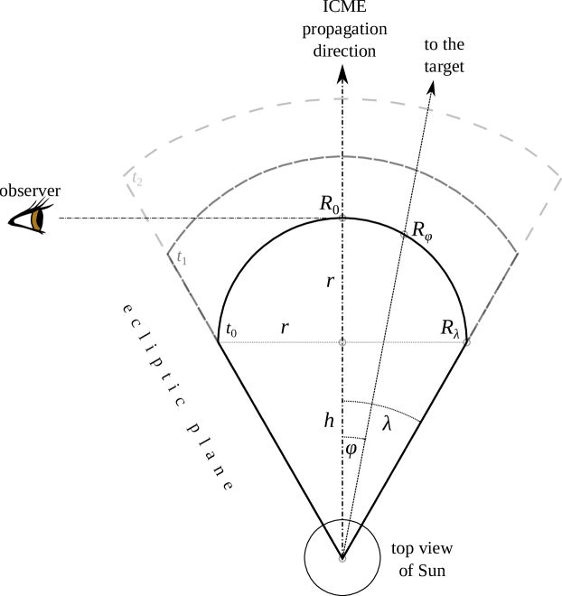
Figure 3: A cross section of a conical representation of a CME in the ecliptic plane during ICME propagation. The simple schematic describes temporal deformation and evolution of the CME’s leading edge in time. The initial CME shape at time $t_{0}$ is defined from a single heliocentric distance measurement $R_{0}$ of the CME tip and used in an equation that defines the conical geometry.

In the current versions of the DBM, implemented as a public prognostic online tool at http://www.geof.unizg.hr/~tzic/dbm.html, the different options of CME expansions are proposed. The prognostic tool forecasts only ICME propagation in the ecliptic plane, as a result of CME initiation at low heliographic latitudes. The geometric setup of the latest online DBM version is presented in Figure 3 where the CME frontal part evolves in time, i.e., the expansion of the CME’s leading edge is simulated by applying the DBM equation of motion, Equation (9), on each leading-edge segment independently. The initial cross section in the ecliptic plane of the CME shape is constructed by a single $R_{0}(0)$ measurement of the CME tip element (which lies on the line of the CME’s propagation direction and in the ecliptic plane as well) and by the assumption of conical CME geometry defined by Equation (A1). The leading edge gradually deforms since different segments are immersed at initial time $t_{0}$ in different surrounding conditions (described by solar wind speed $w(R)$ and $\gamma(R)$ functions) and have different initial velocities (see Equation (A1)), hence the DBM equation of motion results in different radial kinematics. Since the flanks move more slowly, and thus in fast ICMEs the drag-deceleration of flanks is weaker whereas flank acceleration in slow events is stronger, the variation of speed along the ICME front decreases and the front gradually flattens. Note that such an “independent-element” DBM procedure could be equivalently applied to any other presumed initial CME geometry.

References

- Bein et al. (2013) Bein, B. M., Temmer, M., Vourlidas, A., Veronig, A. M., & Utz, D. 2013, ApJ, 768, 31
- Borgazzi et al. (2009) Borgazzi, A., Lara, A., Echer, E., & Alves, M. V. 2009, A&A, 498, 885
- Cargill (2004) Cargill, P. J. 2004, SoPh, 221, 135
- Cargill et al. (1996) Cargill, P. J., Chen, J., Spicer, D. S., & Zalesak, S. T. 1996, JGR, 101, 4855
- Cargill et al. (2000) Cargill, P. J., Schmidt, J., Spicer, D. S., & Zalesak, S. T. 2000, JGR, 105, 7509
- Cargill & Schmidt (2002) Cargill, P. J. & Schmidt, J. M. 2002, AnGp, 20, 879
- Chen (1989) Chen, J. 1989, ApJ, 338, 453
- Chen & Garren (1993) Chen, J. & Garren, D. A. 1993, GeoRL, 20, 2319
- Davies et al. (2012) Davies, J. A., Harrison, R. A., Perry, C. H., et al. 2012, ApJ, 750, 23
- Davis et al. (2010) Davis, C. J., Kennedy, J., & Davies, J. A. 2010, SoPh, 263, 209
- Fisher & Munro (1984) Fisher, R. R. & Munro, R. H. 1984, ApJ, 280, 428
- Gallagher et al. (2003) Gallagher, P. T., Lawrence, G. R., & Dennis, B. R. 2003, ApJL, 588, L53
- Gopalswamy (2006) Gopalswamy, N. 2006, JApA, 27, 243
- Kahler & Webb (2007) Kahler, S. W. & Webb, D. F. 2007, JGRA, 112, 9103
- Lara & Borgazzi (2009) Lara, A. & Borgazzi, A. I. 2009, in IAU Symposium, Vol. 257, IAU Symposium, ed. N. Gopalswamy & D. F. Webb, 287–290
- Leblanc et al. (1998) Leblanc, Y., Dulk, G. A., & Bougeret, J.-L. 1998, SoPh, 183, 165, 10.1023/A:1005049730506
- Liu et al. (2010) Liu, Y., Davies, J. A., Luhmann, J. G., et al. 2010, ApJL, 710, L82
- Lugaz et al. (2010) Lugaz, N., Hernandez-Charpak, J. N., Roussev, I. I., et al. 2010, ApJ, 715, 493
- Lugaz et al. (2009) Lugaz, N., Vourlidas, A., & Roussev, I. I. 2009, AnGp, 27, 3479
- Maričić et al. (2014) Maričić, D., Vršnak, B., Dumbović, M., et al. 2014, SoPh, 289, 351
- Mierla et al. (2010) Mierla, M., Inhester, B., Antunes, A., et al. 2010, AnGp, 28, 203
- Möstl & Davies (2013) Möstl, C. & Davies, J. A. 2013, SoPh, 285, 411
- Motulsky & Ransnas (1987) Motulsky, H. J. & Ransnas, L. A. 1987, FASEB J., 1, 365
- Owens & Cargill (2004) Owens, M. & Cargill, P. 2004, Annales Geophysicae, 22, 661
- Rollett et al. (2014) Rollett, T., Möstl, C., Temmer, M., et al. 2014, ApJL, 790, L6
- Rollett et al. (2012) Rollett, T., Möstl, C., Temmer, M., et al. 2012, SoPh, 276, 293
- Rouillard et al. (2008) Rouillard, A. P., Davies, J. A., Forsyth, R. J., et al. 2008, GeoRL, 35, 10110
- Schwenn et al. (2005) Schwenn, R., dal Lago, A., Huttunen, E., & Gonzalez, W. D. 2005, AnGp, 23, 1033
- Sheeley et al. (1999) Sheeley, N. R., Walters, J. H., Wang, Y.-M., & Howard, R. A. 1999, JGR, 104, 24739
- St. Cyr et al. (2000) St. Cyr, O. C., Plunkett, S. P., Michels, D. J., et al. 2000, JGR, 105, 18169
- Temmer et al. (2011) Temmer, M., Rollett, T., Möstl, C., et al. 2011, ApJ, 743, 101
- Temmer et al. (2012) Temmer, M., Vrsnak, B., Rollett, T., et al. 2012, ApJ, 749, 57
- Thernisien (2011) Thernisien, A. 2011, Astrophys. J. Supp., 194, 33
- Thernisien et al. (2006) Thernisien, A. F. R., Howard, R. A., & Vourlidas, A. 2006, ApJ, 652, 763
- Vourlidas et al. (2011) Vourlidas, A., Howard, R. A., Esfandiari, E., et al. 2011, ApJ, 730, 59
- Vršnak (2001) Vršnak, B. 2001, SoPh, 202, 173
- Vršnak (2006) Vršnak, B. 2006, AdSpR, 38, 431
- Vršnak & Gopalswamy (2002) Vršnak, B. & Gopalswamy, N. 2002, JGRA, 107, 1019
- Vršnak et al. (2004) Vršnak, B., Ruždjak, D., Sudar, D., & Gopalswamy, N. 2004, A&A, 423, 717
- Vršnak et al. (2009) Vršnak, B., Vrbanec, D., Čalogović, J., & Žic, T. 2009, in IAU Symposium, Vol. 257, IAU Symposium, ed. N. Gopalswamy & D. F. Webb, 271–277
- Vršnak & Žic (2007) Vršnak, B. & Žic, T. 2007, A&A, 472, 937
- Vršnak et al. (2010) Vršnak, B., Žic, T., Falkenberg, T. V., et al. 2010, A&A, 512, A43
- Vršnak et al. (2013) Vršnak, B., Žic, T., Vrbanec, D., et al. 2013, SoPh, 285, 295
- Xie et al. (2004) Xie, H., Ofman, L., & Lawrence, G. 2004, JGRA, 109, A03109