Second-order variational problems on Lie groupoids and optimal control applications

Abstract.

In this paper we study, from a variational and geometrical point of view, second-order variational problems on Lie groupoids and the construction of variational integrators for optimal control problems. First, we develop variational techniques for second-order variational problems on Lie groupoids and their applications to the construction of variational integrators for optimal control problems of mechanical systems. Next, we show how Lagrangian submanifolds of a symplectic groupoid gives intrinsically the discrete dynamics for second-order systems, both unconstrained and constrained, and we study the geometric properties of the implicit flow which defines the dynamics in the Lagrangian submanifold. We also study the theory of reduction by symmetries and the corresponding Noether theorem.

Leonardo Colombo

Department of Mathematics

University of Michigan

530 Church Street, 3828 East Hall

Ann Arbor, Michigan, 48109, USA

David Martín de Diego

Instituto de Ciencias Matemáticas (CSIC-UAM-UCM-UC3M)

Calle Nicolás Cabrera 15, Campus UAM, Cantoblanco

Madrid, 28049, Spain

(Communicated by the associate editor name)

1. Introduction

The topic of discrete Lagrangian mechanics concerns the study of certain discrete dynamical systems on manifolds. As the name suggests, these discrete systems exhibit many geometric features which are analogous to those in continuous Lagrangian mechanics. In particular, the discrete dynamics are derived from variational principles, have symplectic or Poisson flow maps, conserve momentum maps associated to Noether-type symmetries, and admit a theory of reduction. While discrete Lagrangian systems are quite mathematically interesting, in their own right, they also have important applications in the design of structure-preserving numerical methods for many dynamical systems in mechanics and optimal control theory.

Numerical methods which are constructed in this way are called variational integrators. This approach to discretizing Lagrangian systems was put forward in papers by Bobenko and Suris [6], Moser and Veselov [60], and others in the early 1990s, and the general theory was developed over the subsequent decade (see Marsden and West [51] for a comprehensive overview).

A. Weinstein [62] observed that these systems could be understood as a special case of a more general theory, describing discrete Lagrangian mechanics on arbitrary Lie groupoids where the Lagrangian function is defined on a Lie groupoid. A Lie groupoid $G$ is a natural generalization of the concept of a Lie group, where now not all elements are composable. The product $gh$ of two elements is only defined on the set of composable pairs $G_{2}=\left\{(g,h)\in G\times G\,|\,\beta(g)=\alpha(h)\right\}$, where $\alpha:G\rightarrow Q$ and $\beta:G\rightarrow Q$ are the source and target maps over a base manifold $Q$. This concept was introduced in differential geometry by Ereshmann in the 1950’s. The infinitesimal version of a Lie groupoid $G$ is the Lie algebroid $\tau_{AG}:AG\rightarrow Q$, which is the restriction of the vertical bundle of $\alpha$ to the submanifold of the identities. This setting is general enough to include the discrete counterparts of several types of fundamental equations in Mechanics as for instance, Euler-Lagrange equations for Lagrangians defined on tangent bundles [51], Euler-Poincaré equations for Lagrangians defined on Lie algebras [49], [50], Lagrange-Poincaré equations for Lagrangians defined on Atiyah bundles, etc. Such discrete counterparts are obtained discretizing the continuous Lagrangian to the corresponding Lie groupoid and then applying a suitable discrete variational principle.

A complete description of the discrete Lagrangian and Hamiltonian mechanics on Lie groupoids was given in the work by Marrero, Martín de Diego and Martínez [41] (see also [42]). Following the program proposed by A. Weinstein [62], in this work, we generalize the theory of discrete second-order Lagrangian mechanics and variational integrators for a second-order discrete Lagrangian $L_{d}:G_{2}\to\mathbb{R}$ in two main directions. First, we develop variational principles for second-order variational problems on Lie groupoids and we show how to apply this theory to the construction of variational integrators for optimal control problems of mechanical systems. Secondly, we show that Lagrangian submanifolds of a symplectic groupoid (cotangent groupoid) give rise to discrete dynamical second-order systems. We also develop a reduction by symmetries, and study the relationship between the dynamics and variational principles for second-order variational problems. Finally we study discrete second-order constrained Lagrangian mechanics on Lie groupoids. The main application of this theory will be systems subjected to constraints and underactuated control systems. Our results in the second part of the paper are based on the papers [41] and [43] but in second-order theories.

There are variational principles which involves higher-order derivatives [4], [9], [22], [23], [24], [25], [39], [47], [52], [54], [55] since from it one can obtain the equations of motion for Lagrangians where the configuration space is a higher-order tangent bundle. The study of higher-order variational systems has regularly attracted a lot of attention from the applied and theoretical points of view (see [37]), but recently, higher-order variational problems have been studied for their important applications in optimal control, aeronautics, robotics, computer-aided design, air traffic control, trajectory planning and computational anatomy.

Since the main applications of higher-order variational problems are second-order problems we will focus our attention in the second-order case along the work, leaving the extension to higher-order case as a straightforward development.

The organization of the paper is as follows. In Section 2 we recall some constructions and results on discrete Mechanics on Lie groupoids which will be used in the next sections. Section 3 is devoted to study variational principles for second-order discrete mechanical systems on Lie groupoids, their extension to the constrained case and the application to the theory of optimal control of mechanical systems and construction of variational integrators. In Section 4 we show how Lagrangian submanifolds of an appropriate symplectic groupoid (cotangent groupoid) give rise to discrete dynamical second-order systems. From such Lagrangian submanifold we obtain the discrete second-order Euler-Lagrange equations on Lie groupoids and such equations correspond with the ones obtained from the variational point of view. We also develop a reduction by symmetries, and we study the relationship between the different dynamics and variational principles for these second-order variational problems. Finally we study discrete constrained second-order Lagrangian mechanics. This allows for systems with arbitrary constraints.

Throughout the paper, we have occasion to draw on certain technical constructions using the theory of Lie algebroids and retraction maps. We provide some supplementary details and discussion of these and an overview on discrete mechanics and higher-order tangent bundles in some Appendices at the end of this paper.

2. Groupoids and discrete mechanics

This section review some results about Lie groupoids and discrete mechanics on Lie groupoids based on [41] and [42].

2.1. Generalities about Lie groupoids

A groupoid is a small category in which every morphism is an isomorphism (i.e. all morphism is invertible). That is,

Definition 2.1.

A groupoid $G$ over a set $Q,$ denoted $G\rightrightarrows Q$, consists of a set of objects $Q$, a set of morphisms $G$, and the following structural maps:

• a source map $\alpha\colon G\rightarrow Q$ and a target map $\beta\colon G\rightarrow Q$. Thus an element $g\in G$ is thought as an arrow from $x=\alpha(g)$ to $y=\beta(g)$ in $Q$.

• an associative multiplication map $m\colon G_{2}\rightarrow G$, $m(g,h)=gh$, with $\alpha(g)=\alpha(gh)$ and $\beta(h)=\beta(gh)$ where

  $$G_{2}:=G\mathrel{{}_{\beta}\times_{\alpha}}G=\left\{\left(g,h\right)\in G\times G\;\middle|\;\beta(g)=\alpha(h)\right\}$$

  is called set of composable pairs defined by $\alpha$ and $\beta$. $gh$ is thought as the composite arrow from $x$ to $z$ if $g$ is an arrow from $x=\alpha(g)$ to $y=\beta(g)=\alpha(h)$ and $h$ is an arrow from $y$ to $\beta(h)=z$.

• an identity map, $\epsilon\colon Q\rightarrow G,$ a section of $\alpha$ and $\beta$, such that for all $g\in G$,

  $$\epsilon\left(\alpha(g)\right)g=g=g\epsilon\left(\beta(g)\right),$$

• an inversion map $i\colon G\rightarrow G$, mapping $g$ into $g^{-1}$, such that for all $g\in G$,

  $$gg^{-1}=\epsilon\left(\alpha(g)\right)\hbox{ and }g^{-1}g=\epsilon\left(\beta(g)\right).$$

Remark 1.

Alternatively, a groupoid can be seen as a weak version of a group, where the multiplication will be defined only for elements in $G_{2}\subset G\times G$. $\diamond$

We will focus on a particular class of groupoids, the Lie groupoids which have a differential structure in addition to their algebraic structure.

Definition 2.2.

A Lie groupoid is a groupoid $G\rightrightarrows Q$ where

1. $G$ and $Q$ are differentiable manifolds,

2. $\alpha,\beta$ are submersions,

3. the multiplication map $m,$ inversion $i$, and identity $\epsilon$, are differentiable.

Remark 2.

In Definition 2.2, $\alpha$ and $\beta$ must be submersions so that $G_{2}$ is a differentiable manifold. From the definition it follows that $m$ is a submersion, $\epsilon$ is an immersion, and $i$ is a diffeomorphism. $\diamond$

If $q\in Q$, $\alpha^{-1}(q)$ and $\beta^{-1}(q)$ will be said the $\alpha$-fiber and $\beta$-fiber of $q$.

Definition 2.3.

Given a groupoid $G\rightrightarrows Q$ and $g\in G$, define the left translation $\ell_{g}\colon\alpha^{-1}\left(\beta(g)\right)\rightarrow\alpha^{-1}\left(\alpha(g)\right)$ and right translation $r_{g}\colon\beta^{-1}\left(\alpha(g)\right)\rightarrow\beta^{-1}\left(\beta(g)\right)$ by $g$ to be

$$\ell_{g}(h)=gh\hbox{ and }r_{g}(h)=hg.$$

Note that, $\ell^{-1}_{g}=\ell_{g^{-1}}$ and $r^{-1}_{g}=r_{g^{-1}}.$

Denoting by $\mathfrak{X}(G)$ the set of vector fields on $G$ one may introduce the notion of a left (right)-invariant vector field in a Lie groupoid, as in the case of Lie groups.

Definition 2.4.

Given a Lie groupoid $G\rightrightarrows Q$, a vector field $X\in\mathfrak{X}(G)$ is left-invariant (resp., right-invariant) if $X$ is $\alpha$-vertical (resp., $\beta$-vertical), that is, it is tangent to the fibers of $\alpha$ (resp., $\beta$), $T\alpha(X)=0$ (resp., $T\beta(X)=0$) and $\left(T_{h}\ell_{g}\right)\left(X(h)\right)=X\left(gh\right)$ for all $(g,h)\in G_{2}$ (resp., $\left(T_{h}r_{g}\right)\left(X(h)\right)=X\left(hg\right)$).

Definition 2.5.

A Lie algebroid $A$ over a manifold $Q$ is a real vector bundle $\tau_{A}:A\to Q$ together with a Lie bracket $[\![\cdot,\cdot]\!]$ on $\Gamma(\tau_{A})$, the set of sections of $\tau_{A}:A\to Q$, and a bundle map $\rho:A\to TQ$ such that $[\![X,fY]\!]=f[\![X,Y]\!]+\rho(X)(f)Y$ for all $X,Y\in\Gamma(\tau_{A})$ and $f\in C^{\infty}(Q)$.

Remark 3.

If $(A,[\![\cdot,\cdot]\!],\rho)$ is a Lie algebroid over $Q$ then $\rho$ is a homomorphism between the Lie algebras $(\Gamma(\tau_{A}),[\![\cdot,\cdot]\!])$ and $(\mathfrak{X}(Q),[\cdot,\cdot])$. $\diamond$

In Lie groups, the infinitesimal version of a Lie group is a Lie algebra, therefore we will see that the corresponding infinitesimal version of a Lie groupoid is a Lie algebroid. Next, we define the Lie algebroid associated with a Lie groupoid $G\rightrightarrows Q$.

Given a Lie groupoid $G\rightrightarrows Q$, consider the vector bundle

$$\tau_{AG}:AG\longrightarrow Q$$

whose fiber at a point $q\in Q$ is $A_{q}G=\ker T_{\epsilon(q)}\alpha=V\alpha$, i.e., the tangent space to the $\alpha$-fiber at the identity section, for $q\in Q$.

It is easy to prove that there exists a bijection between the space of sections $\Gamma\left(\tau_{AG}\right)$ and the set of left-invariant vector fields on $G$. If $X$ is a section of $\tau_{AG}$, the corresponding left-invariant vector field on $G$ will be denoted by $\overleftarrow{X}\in\mathfrak{X}(G)$ where

$$\overleftarrow{X}(g)=\left(T_{\epsilon\left(\beta(g)\right)}\ell_{g}\right)\left(X\left(\beta(g)\right)\right).$$ (1)

The Lie algebroid structure on $AG$ is given by the bracket $[\![\cdot,\cdot]\!]$ and the anchor map $\rho$ defined as follows:

$$\overleftarrow{[\![{X,Y}]\!]}=\bigl{[}\overleftarrow{X},\overleftarrow{Y}\bigr{]},\qquad\rho(X)(q)=\left(T_{\epsilon(q)}\beta\right)\left(X(q)\right),$$ (2)

for all $X,Y\in\Gamma\left(\tau_{AG}\right)$ and $q\in Q$.

Definition 2.6.

Given a Lie groupoid $G\rightrightarrows Q$, the triple $(AG,[\![\cdot,\cdot]\!],\rho)$ defined in (2) is called Lie algebroid associated to $G\rightrightarrows Q$.

Remark 4.

Alternatively one can also establish a bijection between the space of sections $\Gamma\left(\tau_{AG}\right)$ and the set of right-invariant vector fields on $Q$, by

$$\overrightarrow{X}(g)=-\left(T_{\epsilon\left(\alpha(g)\right)}\left(r_{g}\circ i\right)\right)\left(X\left(\alpha(g)\right)\right),$$ (3)

which yields the Lie bracket relation

$$\overrightarrow{[\![{X,Y}]\!]}=-\bigl{[}\overrightarrow{X},\overrightarrow{Y}\bigr{]},\qquad\bigl{[}\overrightarrow{X},\overleftarrow{Y}\bigr{]}=0.$$

Thus the mapping $X$ into $\overleftarrow{X}$ is a Lie algebra isomorphism, and the mapping $X$ into $\overrightarrow{X}$ is a Lie algebra anti-isomorphism (see [20] and [40] fore more details). $\diamond$

2.1.1. Examples of Lie groupoids:

We introduce some examples of Lie groupoids.

$\bullet$ The pair or banal groupoid: Let $Q$ be a differentiable manifold, and consider the product manifold $G=Q\times Q$. $G$ is a Lie groupoid over $Q$ where the source and target maps $\alpha$ and $\beta$ are the projections onto the first and second factors respectively. The identity is defined as $\epsilon(q)=(q,q)$ for all $q\in Q,$ the multiplication $m((q,s),(s,r))=(q,r)$ for $(q,s),(s,r)\in Q\times Q$ and the inverse map $i(q,s)=(s,q).$

Note that, if $q$ is a point of $Q$, then $V_{\epsilon(q)}\alpha\simeq T_{q}Q$. Hence the Lie algebroid of $G$ is isomorphic to the standard Lie algebroid $\tau_{TQ}:TQ\to Q$. In this sense, the Banal groupoid is considered as the discrete space for discretizations of Lagrangian functions $L:TQ\to\mathbb{R}$.

$\bullet$ Lie groups: Let $G$ be a Lie group. $G$ is a Lie groupoid over one point $Q=\{\mathfrak{e}\},$ the identity element of $G.$ The structural maps of the Lie groupoid $G$ are

$$\alpha(g)=\mathfrak{e},\quad\beta(g)=\mathfrak{e},\quad\epsilon(\mathfrak{e})=\mathfrak{e},\quad i(g)=g^{-1}\hbox{ and }m(g,h)=gh,\hbox{ for }g,h\in G.$$

The Lie algebroid associated with $G$ is the Lie algebra $\mathfrak{g}$ of $G$.

$\bullet$ Transformation or action Lie groupoid. Let $H$ be a Lie group with identity $\tilde{\mathfrak{e}}$ and $\varphi:Q\times H\to Q$ be a right action of $H$ on $Q$. The product manifold $G=Q\times H$ is a Lie groupoid over $Q$, with structural maps given by

$$\alpha(q,\tilde{h})=q,\quad\beta(q,\tilde{h})=\varphi(q,\tilde{h}),\quad\epsilon(q)=(q,\tilde{\mathfrak{e}}),\quad m((q,\tilde{h}),(\varphi(q,\tilde{h}),\tilde{h}^{\prime}))=(q,\tilde{h}\tilde{h}^{\prime}),$$

$$i(q,\tilde{h})=(\varphi(q,\tilde{h}),\tilde{h}^{-1})\hbox{ for }q\in Q\hbox{ and }h,h^{\prime}\in H.$$

The Lie groupoid $G$ is called action or transformation Lie groupoid and its associated Lie algebroid is the action algebroid $\hbox{pr}_{1}:M\times\tilde{\mathfrak{h}}\to M$ where $\tilde{\mathfrak{h}}$ is the Lie algebra of the Lie group $H$ (for more details, see [40] and [41]).

$\bullet$ The cotangent groupoid: Let $G\rightrightarrows Q$ be a Lie groupoid. If $A^{\ast}G$ is the dual bundle to $AG$ then the cotangent bundle $T^{\ast}G$ is a Lie groupoid over $A^{\ast}G$. The projections $\tilde{\beta}$ and $\tilde{\alpha}$, the partial multiplication $\oplus_{T^{\ast}G}$, the identity section $\tilde{\epsilon}$ and the inversion $\tilde{\i}$ are defined by the structural maps of $G$ as follows,

$$\kern-15.0pt\begin{array}[]{l}\tilde{\beta}(\mu_{g})(X)=\mu_{g}((T_{\epsilon(\beta(g))}\ell_{g})(X)),\mbox{ for }\mu_{g}\in T^{\ast}_{g}G\mbox{ and }X\in A_{\beta(g)}G,\\[5.0pt] \tilde{\alpha}(\nu_{h})(Y)=\nu_{h}((T_{\epsilon(\alpha(h))}r_{h})(Y-(T_{\epsilon(\alpha(h))}(\epsilon\circ\beta))(Y))),\\[4.0pt] \kern 160.0pt\mbox{ for }\nu_{h}\in T^{\ast}_{h}G\mbox{ and }Y\in A_{\alpha(h)}G,\\[5.0pt] (\mu_{g}\oplus_{T^{\ast}G}\nu_{h})(T_{(g,h)}m(X_{g},Y_{h}))=\mu_{g}(X_{g})+\nu_{h}(Y_{h}),\\[4.0pt] \kern 160.0pt\mbox{ for }(X_{g},Y_{h})\in T_{(g,h)}G_{2},\\[5.0pt] \tilde{\epsilon}(\mu_{x})(X_{\epsilon(x)})=\mu_{x}(X_{\epsilon(x)}-(T_{\epsilon(x)}(\epsilon\circ\alpha))(X_{\epsilon(x)}))),\\[4.0pt] \kern 160.0pt\mbox{ for }\mu_{x}\in A^{\ast}_{x}G\mbox{ and }X_{\epsilon(x)}\in T_{\epsilon(x)}G,\\[5.0pt] \tilde{\i}(\mu_{g})(X_{g^{-1}})=-\mu_{g}((T_{g^{-1}}i)(X_{g^{-1}})),\mbox{ for }\mu_{g}\in T^{\ast}_{g}G\mbox{ and }X_{g^{-1}}\in T_{g^{-1}}G.\end{array}$$ (4)

Here $\alpha,\beta,m,i,\epsilon$ are the structural maps of $G\rightrightarrows Q$ (for more details, see [20] and [31]).

$\bullet$ Symplectic groupoids: Finally, we introduce a subclass of Lie groupoids with an additional structure, symplectic groupoids. They are endowed with a symplectic manifold structure. A symplectic groupoid is a Lie groupoid $G\rightrightarrows Q$ with a symplectic form $\omega$ on $G$ such that the graph of the composition law $m$ given by

$$\hbox{graph}(m):=\{(g,h,r)\in G\times G\times G\mid(g,h)\in G_{2}\hbox{ and }r=m(g,h)\}$$

is a Lagrangian submanifold of $G\times G\times G^{-}$ with the product symplectic form, where the first two factors $G$ are endowed with the symplectic form $\omega$ and the third factor $G^{-}$ with the symplectic form $-\omega.$

Observe that if $G\rightrightarrows Q$ is a Lie groupoid then the cotangent groupoid $T^{*}G\rightrightarrows A^{*}G$ is a symplectic groupoid with the canonical symplectic $2$-form on $T^{*}G$, denoted $\omega_{G}$.

2.2. Lie Groupoids and Discrete Mechanics

Next, we give a review of some generalities on discrete mechanics on Lie groupoids based in [41] and [42].

2.2.1. Discrete Euler-Lagrange equations

Let $G$ be a Lie groupoid over $Q$ with structural maps

$$\alpha,\beta:G\longrightarrow Q,\;\;\epsilon:Q\longrightarrow G,\;\;i:G\longrightarrow G,\;\;m:G_{2}\longrightarrow G.$$

Denote by $\tau_{AG}:AG\to Q$ the Lie algebroid of $G$.

A discrete Lagrangian is a function $\mathbb{L}_{d}:{G}\to\mathbb{R}$. Fixed $g\in G$, we define the set of admissible sequences with values in $G$:

$${\mathcal{C}}^{N}_{g}=\{(g_{1},\ldots,g_{N})\in G^{N}\mid(g_{k},g_{k+1})\in G_{2}\hbox{ for }k=1,\ldots,N-1\hbox{ and }g_{1}\ldots g_{N}=g\}.$$ (5)

An admissible sequence $(g_{1},\dots,g_{N})\in{\mathcal{C}}^{N}_{g}$ is a solution of the discrete Euler-Lagrange equations if

$$0=\sum_{k=1}^{N-1}\left[\overleftarrow{X}_{k}\big{(}{g_{k}})(\mathbb{L}_{d})-\overrightarrow{X}_{k}\big{(}{g_{k+1}})(\mathbb{L}_{d})\right],\;\;\mbox{ for }X_{1},\dots,X_{N-1}\in\Gamma(\tau_{AG}).$$

For $N=2$ we obtain that $(g,h)\in G_{2}$ is a solution of the discrete Euler-Lagrange equations if

$$\overleftarrow{X}({g})(\mathbb{L}_{d})-\overrightarrow{X}({h})(\mathbb{L}_{d})=0$$

for every section $X$ of $AG$.

Remark 5.

Marrero et al. [41] showed that these discrete Euler-Lagrange equations are also equivalent to the sequence $g_{1},\ldots,g_{N}\in G$ corresponding to a critical point of the action sum

$$(g_{1},\ldots,g_{N})\longmapsto\sum_{k=1}^{N}\mathbb{L}_{d}(g_{k}),$$

over the space of admissible sequences.

In the case when $G$ is the banal groupoid $Q\times Q\rightrightarrows Q$, this recovers the discrete Euler-Lagrange equations,

$$D_{1}\mathbb{L}_{d}(q_{k},q_{k+1})+D_{2}\mathbb{L}_{d}(q_{k-1},q_{k})=0$$

for $k=1,\ldots,N-1,$ as in Marsden and West [51]. $\diamond$

2.2.2. Discrete Lagrangian evolution operator

We say that a differentiable mapping $\Psi:G\rightarrow G$ is a discrete flow or a discrete Lagrangian evolution operator for $\mathbb{L}_{d}$ if it verifies the following properties:

1. $\hbox{graph}(\Psi)\subseteq G_{2}$, that is, $(g,\Psi(g))\in G_{2}$, $\forall g\in G$.

2. $(g,\Psi(g))$ is a solution of the discrete Euler-Lagrange equations, for all $g\in G$, that is,

   $$\overleftarrow{X}(g)(\mathbb{L}_{d})-\overrightarrow{X}(\Psi(g))(\mathbb{L}_{d})=0$$ (6)

   for every section $X$ of $AG$ and every $g\in G.$

2.2.3. Discrete Legendre transformations

Given a discrete Lagrangian $\mathbb{L}_{d}:G\to\mathbb{R}$ we define two discrete Legendre transformations $\mathbb{F}^{-}\mathbb{L}_{d}:G\rightarrow A^{*}G$ and $\mathbb{F}^{+}\mathbb{L}_{d}:G\rightarrow A^{*}G$ as follows (see [41])

$$(\mathbb{F}^{-}\mathbb{L}_{d})(h)(v_{\epsilon(\alpha(h))})= -v_{\epsilon(\alpha(h))}(\mathbb{L}_{d}\circ r_{h}\circ i),\mbox{ for }v_{\epsilon(\alpha(h))}\in A_{\alpha(h)}G,$$ (7)

$$(\mathbb{F}^{+}\mathbb{L}_{d})(g)(v_{\epsilon(\beta(g))})= v_{\epsilon(\beta(g))}(\mathbb{L}_{d}\circ\ell_{g}),\mbox{ for }v_{\epsilon(\beta(g))}\in A_{\beta(g)}G.$$ (8)

Note that $(\mathbb{F}^{+}\mathbb{L}_{d})(g)\in A^{*}_{\beta(g)}G$ and $(\mathbb{F}^{-}\mathbb{L}_{d})(h)\in A^{*}_{\alpha(h)}G$.

2.2.4. Regular discrete Lagrangians and Hamiltonian evolution operator

A discrete Lagrangian $\mathbb{L}_{d}:{G}\to\mathbb{R}$ is said to be regular if and only if the Legendre transformation $\mathbb{F}^{+}\mathbb{L}_{d}$ is a local diffeomorphism (equivalently, if and only if the Legendre transformation $\mathbb{F}^{-}\mathbb{L}_{d}$ is a local diffeomorphism). In this case, if $(g_{0},h_{0})\in G\times G$ is a solution of the discrete Euler-Lagrange equations for $\mathbb{L}_{d}$ then, one may prove (see [41]) that there exist two open subsets $U_{0}$ and $V_{0}$ of $G$, with $g_{0}\in U_{0}$ and $h_{0}\in V_{0}$, and there exists a (local) discrete Lagrangian evolution operator $\Psi:U_{0}\to V_{0}$ such that:

1. $\Psi(g_{0})=h_{0}$,

2. $\Psi$ is a diffeomorphism and

3. $\Psi$ is unique, that is, if $U^{\prime}_{0}$ is an open subset of $G$, with $g_{0}\in U_{0}^{\prime},$ and $\Psi^{\prime}:U^{\prime}_{0}\to G$ is a (local) discrete Lagrangian evolution operator then

   $$\Psi\mid_{U_{0}\cap U_{0}^{\prime}}=\Psi^{\prime}\mid_{U_{0}\cap U_{0}^{\prime}}.$$

Moreover, if $\mathbb{F}^{+}\mathbb{L}_{d}$ and $\mathbb{F}^{-}\mathbb{L}_{d}$ are global diffeomorphisms (that is, $\mathbb{L}_{d}$ is hyperregular) then $\Psi=(\mathbb{F}^{-}\mathbb{L}_{d})^{-1}\circ\mathbb{F}^{+}\mathbb{L}_{d}$.

If $\mathbb{L}_{d}:{G}\to\mathbb{R}$ is a hyperregular Lagrangian function, then pushing forward to $A^{*}{G}$ with the discrete Legendre transformations, we obtain the discrete Hamiltonian evolution operator, $\widetilde{\Psi}:A^{*}{G}\to A^{*}{G}$ given by

$$\widetilde{\Psi}=\mathbb{F}^{\pm}\mathbb{L}_{d}\circ\Psi\circ(\mathbb{F}^{\pm}\mathbb{L}_{d})^{-1}\;=\mathbb{F}^{+}\mathbb{L}_{d}\circ(\mathbb{F}^{-}\mathbb{L}_{d})^{-1}.$$ (9)

2.2.5. Example: Discrete Euler-Poincaré equations

Let $G$ be a Lie groupoid over $Q=\{\mathfrak{e}\}$, the identity of $G$. Given $\xi\in{\mathfrak{g}}$ we have the left and right invariant vector fields

$$\overleftarrow{\xi}(g)=(T_{\mathfrak{e}}\ell_{g})(\xi)\hbox{ and }\overrightarrow{\xi}(g)=(T_{\mathfrak{e}}r_{g})(\xi),\;\;\mbox{ for }g\in G.$$

Given a discrete Lagrangian $\mathbb{L}_{d}:G\rightarrow\mathbb{R}$ its discrete Euler-Poincaré equations are

$$(T_{\mathfrak{e}}\ell_{g_{k}})(\xi)(\mathbb{L}_{d})-(T_{\mathfrak{e}}r_{g_{k+1}})(\xi)(\mathbb{L}_{d})=0,\;\hbox{ for all }\xi\in{\mathfrak{g}}\mbox{ and }g_{k},g_{k+1}\in G,$$

that is,

$$(\ell_{g_{k}}^{*}\hbox{d}\mathbb{L}_{d})({\mathfrak{e}})=(r_{g_{k+1}}^{*}\hbox{d}\mathbb{L}_{d})({\mathfrak{e}})$$

(see [6, 49, 50]).

A way to discretize a continuous problem is by using a retraction map $\tau:{\mathfrak{g}}\to G$, which is an analytic local diffeomorphism and maps a neighborhood $V\subseteq\mathfrak{g}$ of $0\in{\mathfrak{g}}$ to a neighborhood $U\subseteq G$ of the identity $\mathfrak{e}\in G$. We have that $\tau(\xi)\tau(-\xi)=\mathfrak{e}$ for all $\xi\in\mathfrak{g}$ (see [7]).

The retraction map provides a local chart on the Lie group and it is used to express a small change in the group configuration through a unique Lie algebra element, namely $\xi_{k}=\tau^{-1}(g_{k}^{-1}g_{k+1})/h$, where $h>0$ is a small enough time step, $\xi_{k}\in\mathfrak{g}$, $h\xi_{k}\in V\subseteq\mathfrak{g}$ and $g_{k},g_{k+1}\in U\subseteq G$, i.e., if $\xi_{k}$ were regarded as an average velocity between $g_{k}$ and $g_{k+1}$, then $\tau$ is an approximation of the corresponding vector field on $G$ (see [33]).

To derive the discrete Euler-Poincaré equations, one uses the left-trivialized tangent retraction map $d\tau_{\xi}:\mathfrak{g}\to\mathfrak{g}$ and its inverse $d\tau_{\xi}^{-1}:\mathfrak{g}\to\mathfrak{g}$ defined by

$$T_{\xi}\,\tau(\eta)= T_{\mathfrak{e}}\ell_{\tau(\xi)}(\hbox{d}\tau_{\xi}(\eta))\equiv\hbox{d}\tau_{\xi}(\eta)\tau(\xi),$$

$$T_{\tau(\xi)}\tau^{-1}((T_{\mathfrak{e}}\ell_{\tau(\xi)})\eta)= \hbox{d}\tau_{\xi}^{-1}(\eta),$$

for $\eta\in\mathfrak{g}$ (see [32], [7]) .

The Lie algebra $\mathfrak{g}$ is on itself a vector space, then it is natural to consider local coordinates on $\mathfrak{g}$. We will write $\tau(h\xi)=g$ for a enough small time step $h>0$ such that $h\xi\subseteq V$ where $V$ is a local neighborhood of $0\in{\mathfrak{g}}$. Fixing a basis $\{e_{\gamma}\}$ of $\mathfrak{g}$ we induce coordinates $(y^{\gamma})$ on $\mathfrak{g}$. In these coordinates, a basis of left-invariant and right-invariant vector fields is

$$\overleftarrow{e_{\gamma}}(\eta) =T_{\tau(h\eta)}\tau^{-1}(\tau(h\eta)e_{\gamma})=\mbox{d}\tau^{-1}_{h\eta}({\rm Ad}_{\tau(h\eta)}e_{\gamma}),$$

$$\overrightarrow{e_{\gamma}}(\eta) =T_{\tau(h\eta)}\tau^{-1}(e_{\gamma}\tau(h\eta))=\mbox{d}\tau^{-1}_{h\eta}(e_{\gamma}),$$

where $\eta\in{\mathfrak{g}}$.

Given a Lagrangian $l:{\mathfrak{g}}\rightarrow\mathbb{R}$, the discrete Euler-Poincaré equations are:

$$\overleftarrow{e_{\gamma}}(\eta_{k})(l)-\overrightarrow{e_{\gamma}}(\eta_{k+1})(l)=0,$$ (10)

that is,

$$(\hbox{d}\tau^{-1}_{h\eta_{k}})^{*}\left(\frac{\partial l}{\partial\xi}(\eta_{k})\right)-(\hbox{d}\tau^{-1}_{-h\eta_{k+1}})^{*}\left(\frac{\partial l}{\partial\xi}(\eta_{k+1})\right)=0,$$

(see [42]).

3. Second-order variational problems on Lie groupoids and optimal control applications

In this section, we discuss discrete second-order Lagrangian mechanics using techniques of variational calculus on Lie groupoids (see [30] and [41] for first order variational calculus on Lie groupoids) and we illustrate our results with some examples and applications in the theory of optimal control of mechanical systems.

3.1. Second-order variational problems on Lie groupoids

Let $G$ be a Lie groupoid with structural maps $\alpha,\beta:G\to Q$, $\epsilon:Q\to G$, $i:G\to G$ and $m:G_{2}\to G$. Denote by $\tau_{AG}:AG\to Q$ the Lie algebroid associated with the Lie groupoid $G$.

Definition 3.1.

A discrete second-order Lagrangian $L_{d}:G_{2}\to\mathbb{R}$ is a differentiable function defined on the set of composable elements describing the dynamics of the mechanical system.

We denote by $G^{4}$ the product $G\times G\times G\times G$. As in the first order case, fixed $g\in G$, we define the set of admissible sequences in $G^{4}$ with values in $G$ by consider $N=4$ in (5), that is,

$$C^{4}_{g}=\{(g_{1},g_{2},g_{3},g_{4})\in G^{4}\mid(g_{k},g_{k+1})\in G_{2}\hbox{ for }k=1,2,3$$

$$\hbox{ with }g_{1}\hbox{ and }g_{4}\hbox{ fixed and }g_{1}g_{2}g_{3}g_{4}=g\}.$$

Given a tangent vector at the point $\bar{g}=(g_{1},g_{2},g_{3},g_{4})$ to the manifold $C^{4}_{g}$, we may write it as the tangent vector at $t=0$ of a curve $c(t)$ in $C^{4}_{g}$, which passes through $\bar{g}$ at $t=0$. This type of curves has the form

$$c(t)=(g_{1},g_{2}h_{2}(t),h_{2}^{-1}(t)g_{3},g_{4}),$$ (11)

where $h_{2}(t)\in\alpha^{-1}(\beta(g_{2}))$, for all $t$, and $h_{2}(0)=\epsilon(\beta(g_{2})).$ The curve $c$ is called a variation of $\bar{g}$. Therefore we may identify the tangent space to $C^{4}_{g}$ at $\bar{g}$ with

$$T_{\bar{g}}C^{4}_{g}\equiv\{v_{2}\mid v_{2}\in A_{x_{2}}G\hbox{ where }x_{2}=\beta(g_{2})\}.$$

The curve $v_{2}$ is called infinitesimal variation of $\bar{g}$ and is the tangent vector to the $\alpha$-vertical curve $h_{2}$ at $t=0$.

We define the discrete action sum associated with the discrete second-order Lagrangian $L_{d}:G_{2}\to\mathbb{R}$ by

$$S_{L_{d}}:C_{g}^{4} \longrightarrow \mathbb{R}$$

$$\bar{g} \longmapsto \sum_{k=1}^{3}L_{d}(g_{k},g_{k+1}).$$ (12)

To derive the discrete equations of motion we apply Hamilton’s principle of critical action. In order to do that, we need to consider the variations of the discrete action sum.

Definition 3.2 (Discrete Hamilton’s principle on Lie groupoids).

Given $g\in G$, an admissible sequence $\bar{g}\in C_{g}^{4}$ is a solution of the Lagrangian system determined by $L_{d}:G_{2}\to\mathbb{R}$ if and only if $\bar{g}$ is a critical point of $S_{L_{d}}$.

Proposition 1.

Given $g\in G$, the admissible sequence $\bar{g}=(g_{1},g_{2},g_{3},g_{4})\in C_{g}^{4}$ is a solution of the Lagrangian system determined by $L_{d}:G_{2}\to\mathbb{R}$ if and only if $\bar{g}$ satisfies the discrete second-order Euler-Lagrange equations for $L_{d}:G_{2}\to\mathbb{R}$ given by

$$\ell^{*}_{g_{2}}\left(D_{1}L_{d}(g_{2},g_{3})+D_{2}L_{d}(g_{1},g_{2})\right)+(r_{g_{3}}\circ i)^{*}\left(D_{1}L_{d}(g_{3},g_{4})+D_{2}L_{d}(g_{2},g_{3})\right)=0.$$ (13)

Proof. By definition (3.2), $\bar{g}$ is a solution of the Lagrangian system determined by $L_{d}:G_{2}\to\mathbb{R}$ if it is a critical point of $S_{L_{d}}$. In order to characterize the critical points, we calculate,

$$\frac{d}{dt}\Big{|}_{t=0}S_{L_{d}}(c(t))=\frac{d}{dt}\Big{|}_{t=0}\{L_{d}(g_{1},g_{2}h_{2}(t))+L_{d}(g_{2}h_{2}(t),h_{2}^{-1}(t)g_{3})+L_{d}(h_{2}^{-1}(t)g_{3},g_{4})\},$$

where $c(t)$ is the variation of $\bar{g}$ defined in (11).

Then, the condition $\displaystyle{\frac{d}{dt}\Big{|}_{t=0}S_{L_{d}}(c(t))=0}$ is equivalent to

$$0= d(L_{d}\circ\ell_{g_{2}})(\epsilon(\beta(g_{2})))(v_{2})+d(L_{d}\circ r_{g_{3}}\circ i)(\epsilon(\beta(g_{2})))(v_{2})$$

$$+d(L_{d}\circ r_{g_{3}}\circ i)(\epsilon(\beta(g_{3})))(v_{2})+d(L_{d}\circ\ell_{g_{2}})(\epsilon(\beta(g_{1})))(v_{2}),$$ (14)

where $v_{2}\in A_{\beta(g_{2})}G$ is the infinitesimal variation of $\bar{g}$, $\epsilon(\beta(g_{2}))=h_{2}(0)$ and $\ell_{g}$ and $r_{g}$ were defined on Definition 2.3.

Therefore, $\bar{g}$ is a solution of the Lagrangian system determined by the discrete second-order Lagrangian $L_{d}:G_{2}\to\mathbb{R}$ if and only if it satisfies equations (3.1), that is, $\bar{g}$ is a solution of the Lagrangian system determined by $L_{d}:G_{2}\to\mathbb{R}$ if and only if $\bar{g}$ satisfies

$$\ell^{*}_{g_{2}}\left(D_{1}L_{d}(g_{2},g_{3})+D_{2}L_{d}(g_{1},g_{2})\right)+(r_{g_{3}}\circ i)^{*}\left(D_{1}L_{d}(g_{3},g_{4})+D_{2}L_{d}(g_{2},g_{3})\right)=0.$$ (15)

$\square$

The equations given above are called discrete second-order Euler-Lagrange equations.

3.1.1. Example: Discrete second-order Euler-Lagrange equations on the pair groupoid.

Let $Q\times Q\rightrightarrows Q$ be the Banal groupoid. An admissible path is the $4$-tuple $((q_{1},q_{2}),(q_{2},q_{3}),(q_{3},q_{4}),(q_{4},q_{5}))\in C^{4}_{(q_{1},q_{5})}$. $(Q\times Q)_{2}$ is isomorphic to $3Q$ where inclusion of $3Q$ into $(Q\times Q)_{2}$ is given by the map $(q,\tilde{q},\bar{q})\hookrightarrow((q,\tilde{q}),(\tilde{q},\bar{q}))$. Applying Hamilton’s principle for the discrete second-order Lagrangian $L_{d}:(Q\times Q)_{2}\simeq 3Q\to\mathbb{R}$ given by $L_{d}((q_{k},q_{k+1}),(q_{k+1},q_{k+2}))=L_{d}(q_{k},q_{k+1},q_{k+2})$, one gets

$$\frac{d}{dt}\Big{|}_{t=0}S_{L_{d}}=\frac{d}{dt}\Big{|}_{t=0}\sum_{k=1}^{3}L_{d}(q_{k},q_{k+1},q_{k+2}).$$

Hence, the path $((q_{1},q_{2}),(q_{2},q_{3}),(q_{3},q_{4}),(q_{4},q_{5}))\in C^{4}_{(q_{1},q_{5})}$ is a critical point of $S_{L_{d}}$ if and only if it satisfies

$$D_{3}L_{d}(q_{1},q_{2},q_{3})+D_{2}L_{d}(q_{2},q_{3},q_{4})+D_{1}L_{d}(q_{3},q_{4},q_{5})=0.$$ (16)

for $(q_{1},q_{2})$ and $(q_{4},q_{5})$ fixed points in the Banal groupoid.

These equations are the discrete second-order Euler-Lagrange equations for $L_{d}:Q\times Q\times Q\to\mathbb{R}$ (see for example [1]).

3.1.2. Example: Discrete second-order Euler-Poincaré equations

Let $G$ be a Lie group, that is $G$ is a Lie groupoid over the identity element $\{\mathfrak{e}\}$ of $G$. Given $g\in G$ and a discrete second-order Lagrangian $L_{d}:G_{2}\to\mathbb{R}$, the solution for the Lagrangian system determined by the discrete Lagrangian $L_{d}$ are

$$0= \ell^{*}_{g_{k}}D_{1}L_{d}(g_{k},g_{k+1})+\ell^{*}_{g_{k}}D_{2}L_{d}(g_{k-1},g_{k})-r^{*}_{g_{k+1}}D_{2}L_{d}(g_{k},g_{k+1})$$

$$-r^{*}_{g_{k+1}}D_{1}L_{d}(g_{k+1},g_{k+2})$$

for an admisible sequence $(g_{k-1},g_{k},g_{k+1},g_{k+2})\in\mathcal{C}^{4}_{g}$ with $g=g_{k-1}g_{k}g_{k+1}g_{k+2}$ and $g_{1},g_{4}$ fixed points in $G$.

The equations given above are the discrete second-order Euler-Poincaré equations (see for example [17] and [9]).

3.1.3. Example: Discrete second-order Euler-Lagrange equations on an action Lie groupoid

Let $H$ be a Lie group, and $Q$ a differentiable manifold. Let $\varphi:Q\times H\to Q$ be a right action, $\varphi(q,h)=qh$. We consider the action Lie groupoid, $G=Q\times H$ over $Q$. The set of composable elements is determined by

$$G_{2}=\{((q_{1},h_{1}),(q_{2},h_{2}))\mid q_{2}=q_{1}h_{1}\}.$$

If $(q,h)\in G$, the left-translation $\ell_{(q,h)}:\alpha^{-1}(qh)\to\alpha^{-1}(q)$ and the right-translation $r_{(q,h)}:\beta^{-1}(q)\to\beta^{-1}(qh)$ (where $\alpha$ and $\beta$ are the source and target map of $G$) are given by $\ell_{(q,h)}(qh,h^{\prime})=(q,hh^{\prime})$ and $r_{(q,h)}(q(h^{\prime})^{-1},h^{\prime})=(q(h^{\prime})^{-1},h^{\prime}h)$ for $q\in Q,h,h^{\prime}\in H$.

Consider an admissible path

$$((q_{1},h_{1}),(q_{1}h_{1},h_{2}),(q_{1}h_{1}h_{2},h_{3}),(q_{1}h_{1}h_{2}h_{3},h_{4}))\in\mathcal{C}_{x}^{4}$$

where $x=(q_{1},h)\in Q\times H$ with $h=h_{1}h_{2}h_{3}h_{4}$ and $(q_{1},h_{1}),(q_{1}h_{1}h_{2}h_{3},h_{4})$ are fixed in $(Q\times H)$. A discrete second-order Lagrangian is defined as $L_{d}:(Q\times H)_{2}\simeq Q\times H\times H\to\mathbb{R}$ by

$$L_{d}(q_{1},h_{1},h_{2}):=L_{d}((q_{1},h_{1}),(q_{1}h_{1},h_{2})).$$

The discrete Euler-Lagrange equations for the system determined by the discrete second-order discrete Lagrangian $L_{d}:Q\times H\times H\to\mathbb{R}$ are determined by

$$0= \ell_{(q_{1}h_{1},h_{2})}^{*}\left(D_{1}L_{d}(q_{1}h_{1},h_{2},h_{3})+D_{2}L_{d}(q_{1}h_{1},h_{2},h_{3})+D_{3}L_{d}(q_{1},h_{1},h_{2})\right)$$

$$+(r_{(q_{1}h_{1}h_{2},h_{3})}\circ i)^{*}\left(D_{1}L_{d}(q_{1}h_{1}h_{2},h_{3},h_{4})+D_{2}L_{d}(q_{1}h_{1}h_{2},h_{3},h_{4})\right.$$

$$\left.+D_{3}L_{d}(q_{1}h_{1},h_{2},h_{3})\right).$$

$$q_{2}= \varphi(q_{1},h_{1}).$$

3.2. Second-order constrained variational problems on Lie groupoids

Next, we extend the previous variational principle to second-order variational problems for systems subject to second-order constraints. The constructions presented here are interesting for applications in optimal control problem of underactuated mechanical controlled systems.

Let $L_{d}:G_{2}\to\mathbb{R}$ be a discrete second-order Lagrangian describing the dynamics of a discrete mechanical system. Suppose that the dynamics is restricted. This restriction is given by the vanishing of $s$ smooth constraint functions $\Phi_{d}^{A}:G_{2}\to\mathbb{R},$ $A=1,\ldots,s$ determining a submanifold $\mathcal{M}$ of $G_{2}$.

The dynamics of the second-order constrained variational problem associated with $L_{d}$ and $\Phi_{d}^{A}$ is described by the discrete constrained second-order Euler-Lagrange equations determined by considering the augmented Lagrangian $\widehat{L}_{d}:G_{2}\times\mathbb{R}^{s}\to\mathbb{R}$ given by $\widehat{L}_{d}=L_{d}+\lambda_{A}\Phi_{d}^{A}$ where $\lambda_{A}=(\lambda_{1},\ldots,\lambda_{s})\in\mathbb{R}^{s}$ are Lagrange multipliers to be determined (see subsection 4.5 for an intrinsic approach).

Given $g\in G$, the set of admissible sequences is given by

$$C^{4}_{g,\mathcal{M}}=\{(g_{1},g_{2},g_{3},g_{4},\lambda^{1},\lambda^{2},\lambda^{3})\in G^{4}\times\mathbb{R}^{3s}\mid(g_{k},g_{k+1})\in G_{2},\Phi_{d}^{A}(g_{k},g_{k+1})=0$$

$$\hbox{ for }k=1,2,3\hbox{ with }g_{1}\hbox{ and }g_{4}\hbox{ fixed and }g_{1}g_{2}g_{3}g_{4}=g\}.$$

Consider the extended action sum associated with the extended Lagrangian $\widehat{L}_{d}:G_{2}\times\mathbb{R}^{s}\to\mathbb{R}$

$$S_{\widehat{L}_{d}}:C_{g,\mathcal{M}}^{4} \longrightarrow \mathbb{R}$$

$$(g_{1},g_{2},g_{3},g_{4},\lambda^{1},\lambda^{2},\lambda^{3}) \longmapsto \sum_{k=1}^{3}\left[L_{d}(g_{k},g_{k+1})+(\lambda^{k}_{A})^{T}\Phi^{A}_{d}(g_{k},g_{k+1})\right]\;,$$ (17)

where $\lambda_{A}^{k}=(\lambda_{1}^{k},\ldots,\lambda_{s}^{k})\in\mathbb{R}^{s}$. An easy adaptation of the variational principle (3.2) for the discrete extended Lagrangian $\widehat{L}_{d}$ can be done to obtain the discrete constrained second-order Euler-Lagrange equations by extremizing the extended action sum $S_{\widehat{L}_{d}}$. The equations describing the dynamics of second-order constrained variational problems are

$$0= \Phi_{d}^{A}(g_{1},g_{2}),\quad 0=\Phi_{d}^{A}(g_{2},g_{3}),\quad 0=\Phi_{d}^{A}(g_{3},g_{4})\hbox{ with }A=1,\ldots,s,$$

$$0= \ell_{g_{2}}^{*}\left(D_{1}L_{d}(g_{2},g_{3})+\lambda^{2}_{A}D_{1}\Phi^{A}_{d}(g_{2},g_{3})+D_{2}L_{d}(g_{1},g_{2})+\lambda^{1}_{A}D_{2}\Phi^{A}_{d}(g_{1},g_{2})\right)$$ (18)

$$+(r_{g_{3}}\circ i)^{*}\left(D_{1}L_{d}(g_{3},g_{4})+\lambda^{3}_{A}D_{1}\Phi^{A}_{d}(g_{3},g_{4})+D_{2}L_{d}(g_{2},g_{3})+\lambda^{2}_{A}D_{2}\Phi^{A}_{d}(g_{2},g_{3})\right).$$

3.3. Application to optimal control of mechanical systems

In this section we study how to apply the second-order Euler-Lagrange equations on Lie groupoids to optimal control problems of mechanical systems defined on Lie algebroids. After introducing optimal control control problems, we study their discretization.

3.3.1. Optimal control problems of total-actuated mechanical systems on Lie algebroids

Let $(A,[\![\cdot,\cdot]\!],\rho)$ be a Lie algebroid over $Q$ with bundle projection $\tau_{A}:A\to Q$. The dynamics is specified fixing a Lagrangian $L:A\to\mathbb{R}$ (see Appendix C) . External forces are modeled, in this case, by curves $u_{F}:\mathbb{R}\to A^{*}$ where $A^{*}$ is the dual bundle $\tau_{A^{*}}:A^{*}\to\ Q$.

Given local coordinates $(q^{i})$ on $Q$, and fixing a basis of sections $\{e_{\alpha}\}$ of $\tau_{A}:A\to Q$ we can induce local coordinates $(q^{i},y^{\alpha})$ on $A$; that is, every element $b\in A_{q}=\tau_{A}^{-1}(q)$ is expressed univocally as $b=y^{\alpha}e_{\alpha}(q)$. The notion of admissible curves replaces that of natural prolongation in the context of Lie algebroids.

Definition 3.3.

Let $(A,[\![\cdot,\cdot]\!],\rho)$ be a Lie algebroid over $Q$ with projection $\tau_{A}:A\to Q$. A curve $\xi:I\subset\mathbb{R}\to A$ is an admissible curve on $A$ if

$$\rho(\xi(t))=\frac{d}{dt}(\tau_{A}(\xi(t))).$$

In a local description, a curve $\xi$ on $A$ given by $\xi(t)=(q^{i}(t),y^{\alpha}(t))$, is admissible if

$$\dot{q}^{i}=\rho_{\alpha}^{i}(q)y^{\alpha}$$

where if $b=y^{\alpha}e_{\alpha}(q)$ with $q=\tau_{AG}(b)$ then $\displaystyle{\rho(b)=\rho_{\alpha}^{i}(q)y^{\alpha}\frac{\partial}{\partial q^{i}}\Big{|}_{q}}$.

It is possible to adapt the derivation of the Lagrange-d’Alembert principle to study fully-actuated mechanical controlled systems on Lie algebroids (see [19] and [48]). Let $q_{0}$ and $q_{T}$ fixed in $Q$, consider an admissible curve $\xi:I\subset\mathbb{R}\to A$ which satisfies the principle

$$0=\delta\int_{0}^{T}L(\xi(t))dt+\int_{0}^{T}\langle u_{F}(t),\eta(t)\rangle dt,$$

where $\eta(t)\in{A}_{\tau_{A}(\xi(t))}$ and $u_{F}(t)\in A^{*}_{\tau_{A}(\xi(t))}$ defines the control force (where we are assuming they are arbitrary). The infinitesimal variations in the variational principle are given by $\delta\xi=\eta^{C}$, for all time-dependent sections $\eta\in\Gamma(\tau_{A})$, with $\eta(0)=0$ and $\eta(T)=0$, where $\eta^{C}$ is a time-dependent vector field on $A$, the complete lift, locally defined by

$$\eta^{C}=\rho_{\alpha}^{i}\eta^{\alpha}\frac{\partial}{\partial q^{i}}+(\dot{\eta}+\mathcal{C}^{\alpha}_{\beta\gamma}\eta^{\beta}y^{\gamma})\frac{\partial}{\partial y^{\alpha}}$$

(see [19], [44], [45] and [46]). Here the structure functions $\mathcal{C}_{\beta\gamma}^{\alpha}$ are determined by $[\![e_{\beta},e_{\gamma}]\!]=\mathcal{C}_{\beta\gamma}^{\alpha}e_{\alpha}$.

From the Lagrange-d’Alembert principle one easily derives the controlled Euler-Lagrange equations by using standard variational calculus

$$\frac{d}{dt}\left(\frac{\partial L}{\partial y^{\alpha}}\right)-\rho_{\alpha}^{i}\frac{\partial L}{\partial q^{i}}+\mathcal{C}_{\alpha\beta}^{\gamma}(q)y^{\beta}\frac{\partial L}{\partial y^{\gamma}}= (u_{F})_{\alpha},$$

$$\frac{dq^{i}}{dt}= \rho_{\alpha}^{i}y^{\alpha}.$$

The control force $u_{F}$ is chosen such that it minimizes the cost functional

$$\int_{0}^{T}C(q^{i},y^{\alpha},(u_{F})_{\alpha})dt,$$

where $C:A\oplus A^{*}\to\mathbb{R}$ is the cost function associated with the optimal control problem.

Therefore, the optimal control problem consists on finding an admissible curve $\xi(t)=(q^{i}(t),y^{\alpha}(t))$ solution of the controlled Euler-Lagrange equations, the boundary conditions and minimizing the cost functional for $C:A\oplus A^{*}\to\mathbb{R}$. This optimal control problem can be equivalently solved as a second-order variational problem by defining the second-order Lagrangian $\widetilde{L}:A^{(2)}\to\mathbb{R}$ as

$$\widetilde{L}(q^{i},y^{\alpha},\dot{y}^{\alpha})=C\left(q^{i},y^{\alpha},\frac{d}{dt}\left(\frac{\partial L}{\partial y^{\alpha}}\right)-\rho_{\alpha}^{i}\frac{\partial L}{\partial q^{i}}+\mathcal{C}_{\alpha\beta}^{\gamma}(q)y^{\beta}\frac{\partial L}{\partial y^{\gamma}}\right).$$ (19)

Here $A^{(2)}$ denotes the set of admissible elements of the Lie algebroid $A$, a subset of $A\times TA$, given by

$$A^{(2)}:=\{(b,v_{b})\in A\times TA\mid\rho(b)=T\tau_{A}(v_{b})\}$$

where $T\tau_{A}:TA\to TQ$ is the tangent map of the bundle projection. $A^{(2)}$ is considered as the substitute of the second-order tangent bundle in classical mechanics [46]. In local coordinates, the set $A^{(2)}$ is characterized by the tuple $(q^{i},y^{\alpha},z^{\alpha},v^{\alpha})\in A\times TA$ such that $y^{\alpha}=z^{\alpha}$. Therefore one can consider local coordinates $(q^{i},y^{\alpha},v^{\alpha})$ on $A^{(2)}$.

The dynamics associated with the second-order Lagrangian $\widetilde{L}:A^{(2)}\to\mathbb{R}$ (and therefore the optimality conditions for the optimal control problem) is given by the second-order Euler-Lagrange equations on Lie algebroids (see for example [12] and [47])

$$0=\frac{d^{2}}{dt^{2}}\left(\frac{\partial\widetilde{L}}{\partial v^{\alpha}}\right)+\mathcal{C}_{\alpha\beta}^{\gamma}(q)y^{\beta}\frac{d}{dt}\left(\frac{\partial\widetilde{L}}{\partial v^{\gamma}}\right)-\frac{d}{dt}\frac{\partial\widetilde{L}}{\partial y^{\alpha}}-\mathcal{C}_{\alpha\beta}^{\gamma}(q)y^{\beta}\frac{\partial\widetilde{L}}{\partial y^{\gamma}}+\rho_{\alpha}^{i}\frac{\partial\widetilde{L}}{\partial q^{i}},$$ (20)

together with the admissibility condition $\displaystyle{\frac{dq^{i}}{dt}=\rho_{\alpha}^{i}y^{\alpha}}.$

Remark 6.

Alternatively, one can define the Lagrangian $\widetilde{L}:A^{(2)}\to\mathbb{R}$ in terms of the Euler-Lagrange operator as

$$\widetilde{L}=C\circ(\tau^{\tiny{A^{(2)}}}_{A}\oplus\mathcal{EL}(L)):A^{(2)}\to\mathbb{R},$$

where $\mathcal{EL}(L):A^{(2)}\to A^{*}$ is the Euler-Lagrange operator which locally reads as

$$\mathcal{EL}(L)=\left(\frac{d}{dt}\frac{\partial L}{\partial y^{\alpha}}-\rho_{\alpha}^{i}\frac{\partial L}{\partial q^{i}}+\mathcal{C}_{\alpha\beta}^{\gamma}(q)y^{\beta}\frac{\partial L}{\partial y^{\gamma}}\right)e^{\alpha}.$$

Here $\{e^{\alpha}\}$ is the dual basis of $\{e_{\alpha}\},$ the basis of sections of $A$ and $\tau^{\tiny{A^{(2)}}}_{A}:A^{(2)}\to A$ is the canonical projection between $A^{(2)}$ and $A$ given by the map $A^{(2)}\ni(q^{i},y^{\alpha},v^{\alpha})\mapsto(q^{i},y^{\alpha})\in A.$ $\diamond$

3.3.2. Optimal control problems of underactuated mechanical systems on Lie algebroids

Now, suppose that our mechanical control system is underactuated, that is, the number of control inputs is less than the dimension of the configuration space. The class of underactuated mechanical systems are abundant in real life for different reasons; for instance, as a result of design choices motivated by the search of less cost engineering devices or as a result of a failure regime in fully actuated mechanical systems. Underactuated systems include spacecrafts, underwater vehicles, mobile robots, helicopters, wheeled vehicles and underactuated manipulators. We will see that the corresponding optimality conditions are given by the solutions of second-order constrained Euler-Lagrange equations (see [16]).

Given a Lagrangian function $L:A\to\mathbb{R}$ and control external forces, the controlled equations for an underactuated system defined on a Lie algebroid are

$$\frac{d}{dt}\left(\frac{\partial L}{\partial y^{a}}\right)-\rho_{a}^{i}\frac{\partial L}{\partial q^{i}}+\mathcal{C}_{a\beta}^{\gamma}(q)y^{\beta}\frac{\partial L}{\partial y^{\gamma}}= (u_{F})_{a},$$

$$\frac{d}{dt}\left(\frac{\partial L}{\partial y^{A}}\right)-\rho_{A}^{i}\frac{\partial L}{\partial q^{i}}+\mathcal{C}_{A\beta}^{\gamma}(q)y^{\beta}\frac{\partial L}{\partial y^{\gamma}}= 0,$$

$$\frac{dq^{i}}{dt}= \rho_{\alpha}^{i}y^{\alpha},$$

with $\{\alpha\}=\{A,a\}$. The optimal control problem consists on finding an admissible trajectory $\xi(t)=(q^{i}(t),y^{A}(t),y^{a}(t))$ solution of the controlled Euler-Lagrange equations given boundary conditions and minimizing a cost functional $C:A\oplus A^{*}\to\mathbb{R}$.

This optimal control problem can be solved as a constrained second-order variational problem on Lie algebroids where the second-order Lagrangian $\widetilde{L}:A^{(2)}\to\mathbb{R}$ is given by

$$\widetilde{L}(q^{i},y^{\alpha},v^{a},v^{A})=C\left(q^{i},y^{\alpha},\frac{d}{dt}\left(\frac{\partial L}{\partial y^{a}}\right)-\rho_{a}^{i}\frac{\partial L}{\partial q^{i}}+\mathcal{C}_{a\beta}^{\gamma}(q)y^{\beta}\frac{\partial L}{\partial y^{\gamma}}\right)$$ (21)

and where the dynamics is restricted by the second order constraints

$$\Phi^{A}(q^{i},y^{\alpha},v^{a},v^{A})=\frac{d}{dt}\left(\frac{\partial L}{\partial y^{A}}\right)-\rho_{A}^{i}\frac{\partial L}{\partial q^{i}}+\mathcal{C}_{A\beta}^{\gamma}(q)y^{\beta}\frac{\partial L}{\partial y^{\gamma}}=0.$$

The optimality conditions for the optimal control problem are determined by the second-order constrained Euler-Lagrange equations given by considering the extended Lagrangian $\widehat{L}=\widetilde{L}+\lambda_{A}\Phi^{A}:A^{(2)}\times\mathbb{R}^{s}\to\mathbb{R}$ where $\lambda_{A}=(\lambda_{1},\ldots,\lambda_{s})\in\mathbb{R}^{s}$ are the Lagrange multipliers. These equations are given by (see [12] for more details)

$$0= \frac{d^{2}}{dt^{2}}\left(\frac{\partial\widetilde{L}}{\partial v^{\alpha}}+{\lambda}_{A}\frac{\partial\Phi^{A}}{\partial v^{\alpha}}\right)+\mathcal{C}_{\alpha\beta}^{\gamma}(q)y^{\beta}\frac{d}{dt}\left(\frac{\partial\widetilde{L}}{\partial v^{\gamma}}+{\lambda}_{A}\frac{\partial\Phi^{A}}{\partial v^{\gamma}}\right)-\frac{d}{dt}\frac{\partial\widetilde{L}}{\partial y^{\alpha}}$$

$$-{\lambda}_{A}\frac{\partial\Phi^{A}}{\partial y^{\alpha}}-\mathcal{C}_{\alpha\beta}^{\gamma}(q)y^{\beta}\left(\frac{\partial\widetilde{L}}{\partial y^{\gamma}}+{\lambda}_{A}\frac{\partial\Phi^{A}}{\partial y^{\gamma}}\right)+\rho_{\alpha}^{i}\left(\frac{\partial\widetilde{L}}{\partial q^{i}}+{\lambda}_{A}\frac{\partial\Phi^{A}}{\partial q^{i}}\right),$$

$$0= \Phi^{A}(q^{i},y^{\alpha},v^{\alpha})$$

together with the admissibility condition $\dot{q}^{i}=\rho_{\alpha}^{i}y^{\alpha}$

3.3.3. Optimal control problems on Lie groupoids

Now we describe the discrete optimal control problem on a Lie groupoid $G$. Let $\mathbb{L}_{d}:G\to\mathbb{R}$ be a discrete Lagrangian, an approximation of the action corresponding to a continuous Lagrangian $L:A\to\mathbb{R}$ defined on a Lie algebroid $A$, that is,

$$\mathbb{L}_{d}(g_{k})\simeq\int_{kh}^{(k+1)h}L(\xi(t))dt$$

where $h>0$ is the time step with $T=Nh$ and $\xi$ is an admissible curve on $A$.

The discrete controlled Euler-Lagrange equations are

$$\ell_{g_{k}}^{*}\hbox{d}\mathbb{L}_{d}(g_{k})-(r_{g_{k+1}}\circ i)^{*}\hbox{d}\mathbb{L}_{d}(g_{k+1})=u_{k}\in A^{*}_{\beta(g_{k})}G,$$ (22)

for $k=1,\ldots,N-1$ where $g_{0}$ and $g_{N}$ are fixed on $G$.

We define the subset $G_{\beta}\times_{\tau_{A^{*}G}}A^{*}G$ of $G\times A^{*}G$,

$$G_{\beta}\times_{\tau_{A^{*}G}}A^{*}G:=\{(g,u)\in G\times A^{*}G\mid\beta(g)=\tau_{A^{*}G}(u)\}.$$

Given a discrete cost function $C_{d}:G_{\beta}\times_{\tau_{A^{*}G}}A^{*}G\to\mathbb{R}$, the discrete optimal control problem is determined by extremizing the discrete cost functional

$$\mathcal{J}_{d}(g_{0},g_{1},\ldots,g_{N}):=\sum_{k=0}^{N-1}C_{d}(g_{k},u_{k}),$$ (23)

for $(g_{0},g_{1},\ldots,g_{N})\in G^{N+1}$, satisfying equations (22) with $(g_{k},g_{k+1})\in G_{2}$, $k=0,\ldots,N-1$ and with $g_{0},g_{1},g_{N-1},g_{N}$ and $g=g_{0}g_{1}\ldots g_{N}\in G$ fixed points on $G$.

Defining the discrete second-order Lagrangian $L_{d}:G_{2}\to\mathbb{R}$ as

$$L_{d}(g_{k},g_{k+1}):=C_{d}\left(g_{k},\ell_{g_{k}}^{*}\hbox{d}\mathbb{L}_{d}(g_{k})-(r_{g_{k+1}}\circ i)^{*}\hbox{d}\mathbb{L}_{d}(g_{k+1})\right),$$ (24)

the discrete optimal control problem consists on finding a path $(g_{0},g_{1},\ldots,g_{N})\in G^{N+1}$ minimizing the discrete action sum $\mathcal{J}_{d}$ for the discrete second-order Lagrangian $L_{d}:G_{2}\to\mathbb{R}$ where $g_{0},g_{1},g_{N-1},g_{N}$ and $g=g_{0}g_{1}\ldots g_{N}\in G$ are fixed points in $G.$

Discrete Hamilton’s principle (3.2) states that the paths minimizing $\mathcal{J}_{d}$ subject fixed points $g_{0},g_{1},g_{N-1},g_{N}\in G$ satify the discrete second-order Euler-Lagrange equations for $L_{d}:G_{2}\to\mathbb{R}$ given by

$$0= \ell^{*}_{g_{k}}\left(D_{1}L_{d}(g_{k},g_{k+1})+D_{2}L_{d}(g_{k-1},g_{k})\right)$$

$$+(r_{g_{k+1}}\circ i)^{*}\left(D_{1}L_{d}(g_{k+1},g_{k+2})+D_{2}L_{d}(g_{k},g_{k+1})\right).$$

Therefore, as in the continuous problem, the optimality conditions for the discrete optimal control problem are determined by the discrete second-order Euler-Lagrange equations for $L_{d}:G_{2}\to\mathbb{R}$.

Alternatively, one can start with a continuous optimal control problem associated to a Lagrangian $L:A\to\mathbb{R}$ defined on a Lie algebroid $A$. The optimality conditions for this optimal control problem are determined by a system of fourth order differential equations obtained from the second-order Euler-Lagrange equations associated with the Lagrangian $\widetilde{L}:A^{(2)}\to\mathbb{R}$ determined by the cost function as in (21). Now, we take directly a discretization of the second-order Lagrangian $\widetilde{L}$ to derive $L_{d}:G_{2}\to\mathbb{R}$.

Finally, we would like to point out that the underactuated case follows as in the continuous case by consider a discrete second-order constrained problem as in Subsection 3.2 and the optimality conditions are given by the solutions of the discrete second-order constrained Euler-Lagrange equations (3.2). We will illustrate this in Example 3.3.5.

3.3.4. An illustrative example: Optimal control of a rigid body on SO(3)

In this example, we show how the optimal control problem of a rigid body defined on the Lie group $SO(3)$ can be studied using the previous constructions given before. This example is motivated by the attitude optimal control of spacecrafts (see [35], [36] and references therein).

The Lie groupoid structure of $SO(3)$ over the identity matrix Id is given by

$$\alpha(R)=Id,\quad\beta(R)=Id,\quad\epsilon(Id)=Id,\quad i(R)=R^{-1}\hbox{ and }m(RG)=RG$$

for $R,G\in SO(3).$ The Lie algebroid associated with the Lie groupoid $SO(3)$ is the Lie algebra $\mathfrak{so}(3)$ over a single point, where the anchor map is zero and the bracket is the usual commutator of matrices and the set of admissible elements is identified with $\mathfrak{so}(3)\times\mathfrak{so}(3)$. Observe that, in this case, all the elements are composable, that is, $SO(3)_{2}=SO(3)\times SO(3)$.

The equations of motion of the controlled rigid body are

$$\dot{\Omega}_{1}=P_{1}\Omega_{2}\Omega_{3}+u_{1},\quad\dot{\Omega}_{2}=P_{2}\Omega_{1}\Omega_{3}+u_{2},\quad\dot{\Omega}_{3}=P_{3}\Omega_{1}\Omega_{2}+u_{3},$$ (25)

where $\Omega=(\Omega_{1},\Omega_{2},\Omega_{3})\in\mathbb{R}^{3}$ and $\dot{\Omega}=(\dot{\Omega}_{1},\dot{\Omega}_{2},\dot{\Omega}_{3})\in\mathbb{R}^{3}$, $u_{i}$ are the control inputs (torques for the rigid body) for $i=1,2,3$ and

$$P_{1}=\frac{I_{1}}{I_{2}-I_{3}},\quad P_{2}=\frac{I_{2}}{I_{3}-I_{1}},\quad P_{3}=\frac{I_{3}}{I_{1}-I_{2}},$$

are constants determined by the moments of inertia of the rigid body $I_{1},I_{2},I_{3}$. Here, we are using the typical identification of the Lie algebra $\mathfrak{so}(3)$ with $\mathbb{R}^{3}$ by the hat map $\hat{\cdot}:\mathbb{R}^{3}\to\mathfrak{so}(3)$ (see [2] and [29] for example), where with some abuse of notation, we directly identify $\mathbb{R}^{3}$ with $\mathfrak{so}(3)$ by omitting the hat notation.

Our fixed boundary conditions for the optimal control problem are $(R(0),\Omega(0))$ and $(R(T),\Omega(T))$, where $R(t)\in SO(3)$ is the attitude of the rigid body subject to the reconstruction equation $\dot{R}=R\Omega$ and variations for the attitude are given by $\delta R=R\eta$, with $\eta$ an arbitrary curve on $\mathfrak{so}(3)$. Consider the cost functional

$$\mathcal{J}=\frac{1}{2}\int^{T}_{0}\left(u_{1}^{2}+u_{2}^{2}+u_{3}^{3}\right)\,dt.$$

From eqs. (25) we can work out $u_{1}$, $u_{2}$ and $u_{3}$ in terms of $\Omega$ and $\dot{\Omega}$. Consequently, we can define the function $\widetilde{L}:\mathfrak{so}(3)\times\mathfrak{so}(3)\to\mathbb{R}$ by $\widetilde{L}(\Omega,\dot{\Omega})=\frac{1}{2}u(\Omega,\dot{\Omega})\cdot u(\Omega,\dot{\Omega})$ where $u=(u_{1},u_{2},u_{3})$. Therefore, the Lagrangian function $\widetilde{L}:\mathfrak{so}(3)\times\mathfrak{so}(3)\to\mathbb{R}$ is

$$\widetilde{L}(\Omega,\dot{\Omega})=\frac{1}{2}\left(\left(\dot{\Omega}_{1}-P_{1}\Omega_{2}\Omega_{3}\right)^{2}+\left(\dot{\Omega}_{2}-P_{2}\Omega_{1}\Omega_{3}\right)^{2}+\left(\dot{\Omega}_{3}-P_{3}\Omega_{1}\Omega_{2}\right)^{2}\right).$$ (26)

From (26) the cost functional becomes into $\displaystyle{\mathcal{J}=\int^{T}_{0}\widetilde{L}(\Omega,\dot{\Omega})\,dt,}$ (see [16] for the solution of this second-order variational problem in the continuous setting).

Angular velocities and angular accelerations can be approximated by discrete trajectories $\xi_{k+1/2}\simeq\Omega(kh)$ and $\xi_{k,k+1}\simeq\dot{\Omega}(kh)$ respectively for $\xi_{k},\xi_{k+1}\in\mathfrak{so}(3)$ where $h>0$ is a fixed real number and $T=kh$ with $k=0,\ldots,N$, where we are using the notation $\xi_{k+1/2}=\frac{1}{2}(\xi_{k}+\xi_{k+1})$ and $\xi_{k,k+1}=\frac{1}{h}(\xi_{k+1}-\xi_{k})$. Define the second-order Lagrangian $\mathcal{L}:\mathfrak{so}(3)\times\mathfrak{so}(3)\to\mathbb{R}$ by $\mathcal{L}(\xi_{k},\xi_{k+1})=\widetilde{L}\left(\xi_{k+1/2},\xi_{k,k+1}\right)$.

The optimal control problem, is given by minimizing the cost function associated with the discrete second-order Lagrangian $L_{d}:SO(3)\times SO(3)\to\mathbb{R}$ over discrete paths on $SO(3)$ where

$$L_{d}(w_{k},w_{k+1})=h\mathcal{L}(\mbox{cay}^{-1}(w_{k}),\mbox{cay}^{-1}(w_{k+1})).$$ (27)

Here $(w_{k},w_{k+1})\in SO(3)\times SO(3)$, $\mbox{cay}(h\xi_{k})=w_{k}$ and $\mbox{cay}:\mathfrak{so}(3)\to SO(3)$ denote the Cayley map for the Lie group $SO(3)$ (see Appendix D).

Therefore, the discrete Lagrangian is now given by

$$L_{d}(w_{k},w_{k+1})=h\widetilde{L}\left(\frac{\mbox{cay}^{-1}(w_{k})+\mbox{cay}^{-1}(w_{k+1})}{2h},\frac{\mbox{cay}^{-1}(w_{k+1})-\mbox{cay}^{-1}(w_{k})}{h^{2}}\right).$$

The variational integrator for the optimal control problem is given by applying discrete Hamilton’s principle (3.2) in the discrete action sum determined by the discrete cost

$$\mathcal{C}_{d}=\sum_{k=0}^{N-1}L_{d}(w_{k},w_{k+1}).$$ (28)

Instead of working with the discrete sum (28) one can take

$$\mathcal{C}_{d}=\sum_{k=0}^{N-1}\widetilde{L}\left(\xi_{k+1/2},\xi_{k,k+1}\right)$$ (29)

in order to work in a vector space where variations of $\xi_{k}=\mbox{cay}^{-1}(w_{k})\in\mathfrak{so}(3)$ are given by (see for example [34])

$$\delta\xi_{k} = \frac{1}{h}\left(\mbox{Ad}_{w_{k}}\eta_{k+1}-\eta_{k}+\frac{h}{2}\mbox{ad}_{\xi_{k}}\eta_{k}-\frac{h}{2}\mbox{ad}_{\xi_{k}}(\mbox{Ad}_{w_{k}}\eta_{k+1})+\frac{h^{2}}{4}\xi_{k}\eta_{k}\xi_{k}\right.$$ (30)

$$-\left.\frac{h^{2}}{4}\xi_{k}(\mbox{Ad}_{w_{k}}\eta_{k+1})\xi_{k}\right).$$

3.3.5. Example: optimal control of a heavy top with two internal rotors

The following example illustrates the study of underactuated mechanical control systems on Lie algebroids and the construction of variational integrators for such systems. It is the optimal control problem of the upright spinning of the heavy top (see [11] and reference therein).

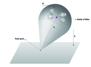
Figure 1. Heavy top with two rotors, each consisting of two rigidly coupled disks.

Consider the top with two rotors so that each rotor’s rotation axis is parallel to the first and the second principal axes of the top as in Figure 1. Let $I_{1},I_{2},I_{3}$ be the moments of inertia of the top in the body fixed frame. Let $J_{1},J_{2}$ be the moments of inertia of the rotors around their rotation axes and $J_{j1},J_{j2},J_{j3}$ be the moments of inertia of the $j$-th rotor, with $j=1,2$, around the first, the second and the third principal axes, respectively. Also we define the quantities $\bar{I}_{1}=I_{1}+J_{11}+J_{21},$ $\bar{I}_{2}=I_{2}+J_{12}+J_{22},$ $\bar{I}_{3}=I_{3}+J_{13}+J_{23},$ $\gamma_{1}=\bar{I}_{1}+J_{1}$ and $\gamma_{2}=\bar{I}_{2}+J_{2}.$

Let $M$ be the total mass of the system, $g$ the magnitude of the gravitational acceleration and $h$ the distance from the origin to the center of mass of the system.

The system is modeled on the transformation Lie algebroid $A=\mathbb{R}^{3}\times\mathfrak{so}(3)\times T(\mathbb{S}^{1}\times\mathbb{S}^{1})$ over the manifold $Q=\mathbb{R}^{3}\times(\mathbb{S}^{1}\times\mathbb{S}^{1})$, where the anchor map $\rho:\mathbb{R}^{3}\times\mathfrak{so}(3)\times T(\mathbb{S}^{1}\times\mathbb{S}^{1})\to T(\mathbb{R}^{3}\times\mathbb{S}^{1}\times\mathbb{S}^{1})$ is locally given by

$$\rho(\Gamma,\Omega,\theta_{1},\theta_{2},\dot{\theta}_{1},\dot{\theta}_{2})=(\Gamma,\theta_{1},\theta_{2},\Gamma\times\Omega,\dot{\theta}_{1},\dot{\theta}_{2}).$$

Here $\Omega=(\Omega_{1},\Omega_{2},\Omega_{3})\in\mathfrak{so}(3)\simeq\mathbb{R}^{3}$ is the angular velocity of the top in the body fixed frame, $\Gamma=(\Gamma_{1},\Gamma_{2},\Gamma_{3})\in\mathbb{R}^{3}$ represents the unit vector with the direction opposite to the gravity as seen from the body and $\theta=(\theta_{1},\theta_{2})$ is the rotation angle of rotors around their axes.

If we denote by $E_{i}$ $(i=1,2,3),$ the standard basis of matrices of $\mathfrak{so}(3),$ given by

$$E_{1}=\left(\begin{array}[]{ccc}0&0&0\\ 0&0&-1\\ 0&1&0\\ \end{array}\right),\quad E_{2}=\left(\begin{array}[]{ccc}0&0&1\\ 0&0&0\\ -1&0&0\\ \end{array}\right),\quad E_{3}=\left(\begin{array}[]{ccc}0&-1&0\\ 1&0&0\\ 0&0&0\\ \end{array}\right)$$

then the basis of sections of $A$ is given by the elements

$$X^{E_{i}}(\Gamma,\theta_{1},\theta_{2}) =\left(\Gamma,E_{i},\theta_{1},\theta_{2},0,0\right),$$

$$X^{\theta_{1}}(\Gamma,\theta_{1},\theta_{2}) =\left(\Gamma,0,\theta_{1},\theta_{2},1,0\right),$$

$$X^{\theta_{1}}(\Gamma,\theta_{1},\theta_{2}) =\left(\Gamma,0,\theta_{1},\theta_{2},0,1\right)$$

with $i=1,2,3$.

The Lie bracket of sections of $A$ is determined by

$$[\![X^{E_{1}},X^{E_{2}}]\!] =X^{[E_{1},E_{2}]}=X^{E_{3}},$$

$$[\![X^{E_{1}},X^{E_{3}}]\!] =X^{[E_{1},E_{3}]}=-X^{E_{2}},$$

$$[\![X^{E_{2}},X^{E_{3}}]\!] =X^{[E_{2},E_{3}]}=X^{E_{1}},$$

$$[\![X^{\theta_{r}},X^{\theta_{s}}]\!] =0,$$

with $r,s=1,2$ and $[\![X^{\theta_{s}},X^{E_{i}}]\!]=0,$ for $s=1,2$ and $i=1,2,3$.

The reduced Lagrangian $l:\mathbb{R}^{3}\times\mathfrak{so}(3)\times T(\mathbb{S}^{1}\times\mathbb{S}^{1})\to\mathbb{R}$ is given by

$$l(\Gamma,\Omega,\dot{\theta})=\frac{1}{2}\left(\begin{array}[]{c}\Omega_{1}\\ \Omega_{2}\\ \Omega_{3}\\ \dot{\theta}_{1}\\ \dot{\theta}_{2}\\ \end{array}\right)^{T}\left(\begin{array}[]{ccccc}\gamma_{1}&0&0&J_{1}&0\\ 0&\gamma_{2}&0&0&J_{2}\\ 0&0&\bar{I}_{3}&0&0\\ J_{1}&0&0&J_{1}&0\\ 0&J_{2}&0&0&J_{2}\\ \end{array}\right)\left(\begin{array}[]{c}\Omega_{1}\\ \Omega_{2}\\ \Omega_{3}\\ \dot{\theta}_{1}\\ \dot{\theta}_{2}\\ \end{array}\right)-Mgh\Gamma_{3}.$$

The Euler-Lagrange equations for $l$ are given by

$$\frac{d}{dt}\left(\frac{\partial l}{\partial\Omega}\right) =\frac{\partial l}{\partial\Omega}\times\Omega+Mgh\Gamma\times e_{3},$$

$$\frac{d}{dt}\left(\frac{\partial l}{\partial\dot{\theta}_{i}}\right) =0,\quad i=1,2;$$

together with the admissibility condition $\dot{\Gamma}=\Gamma\times\Omega.$

Next, we add controls in our picture. Each rotor can be controlled is such way the controlled Euler-Lagrange equations are now

$$\frac{d}{dt}\left(\frac{\partial l}{\partial\Omega}\right)= \frac{\partial l}{\partial\Omega}\times\Omega+Mgh\Gamma\times e_{3},$$

$$\frac{d}{dt}\left(\frac{\partial l}{\partial\dot{\theta}_{i}}\right)= u_{i},\quad i=1,2;$$

$$\dot{\Gamma}= \Gamma\times\Omega.$$

where $e_{3}=(0,0,1)$. That is,

$$\gamma_{1}\dot{\Omega}_{1}+J_{1}\ddot{\theta}_{1}-\gamma_{2}\Omega_{2}\Omega_{3}+\dot{\Omega}_{3}\bar{I}_{3}\Omega_{2}= Mgh\Gamma_{2},$$

$$\gamma_{2}\dot{\Omega}_{2}+J_{2}\ddot{\theta}_{2}+\gamma_{1}\Omega_{1}\Omega_{3}-J_{1}\dot{\theta}_{1}\Omega_{3}= -Mgh\Gamma_{1},$$

$$\bar{I}_{3}\dot{\Omega}_{3}-\gamma_{1}\Omega_{1}\Omega_{2}-J_{1}\dot{\theta}_{1}\Omega_{2}+\gamma_{2}\Omega_{2}\Omega_{1}+J_{2}\dot{\theta}_{2}\Omega_{1}= 0,$$

$$J_{1}(\dot{\Omega}_{1}+\ddot{\theta}_{1})= u_{1},$$

$$J_{2}(\dot{\Omega}_{2}+\ddot{\theta}_{2})= u_{2},$$

together with the admissibility conditions

$$\dot{\Gamma}_{1}=\Gamma_{2}\Omega_{3}-\Gamma_{3}\Omega_{2},\quad\dot{\Gamma}_{2}=\Gamma_{3}\Omega_{1}-\Gamma_{1}\Omega_{3},\quad\dot{\Gamma}_{3}=\Gamma_{1}\Omega_{2}-\Gamma_{2}\Omega_{1}$$

where $\Gamma=(\Gamma_{1},\Gamma_{2},\Gamma_{3})\in\mathbb{R}^{3}.$

The optimal control problem consists on finding an admissible curve $\gamma(t)=(\Gamma(t),\Omega(t),\theta(t),u_{i}(t))$ of the state variables and control inputs, satisfying the controlled equations given above, the boundary conditions and minimizing the cost functional

$$\mathcal{J}=\frac{1}{2}\int_{0}^{T}\left(u_{1}^{2}+u_{2}^{2}\right)dt.$$

This optimal control problem is equivalent to solve the second-order variational problem determined by

$$\min_{(\Omega(\cdot),\theta(\cdot),u(\cdot))}\int_{0}^{T}\widetilde{L}\left(\Omega,\theta,\dot{\Omega},\dot{\theta},\ddot{\theta}\right)dt,$$

and subjected to the second-order constraints $\Phi^{A}:\mathbb{R}^{3}\times\mathbb{R}^{3}\times 2\mathfrak{so}(3)\times T^{(2)}(\mathbb{S}^{1}\times\mathbb{S}^{1})\to\mathbb{R},$ $A=1,\ldots,3$;

$$\Phi^{1}\left(\Omega,\theta,\Gamma,\dot{\Omega},\dot{\theta},\dot{\Gamma},\ddot{\theta}\right)= \gamma_{1}\dot{\Omega}_{1}+J_{1}\ddot{\theta}_{1}-\gamma_{2}\Omega_{2}\Omega_{3}+\dot{\Omega}_{3}\bar{I}_{3}\Omega_{2}-Mgh\Gamma_{2}=0,$$

$$\Phi^{2}\left(\Omega,\theta,\Gamma,\dot{\Omega},\dot{\theta},\dot{\Gamma},\ddot{\theta}\right)= \gamma_{2}\dot{\Omega}_{2}+J_{2}\ddot{\theta}_{2}+\gamma_{1}\Omega_{1}\Omega_{3}-J_{1}\dot{\theta}_{1}\Omega_{3}+Mgh\Gamma_{1}=0,$$

$$\Phi^{3}\left(\Omega,\theta,\Gamma,\dot{\Omega},\dot{\theta},\dot{\Gamma},\ddot{\theta}\right)= \bar{I}_{3}\dot{\Omega}_{3}-\gamma_{1}\Omega_{1}\Omega_{2}-J_{1}\dot{\theta}_{1}\Omega_{2}+\gamma_{2}\Omega_{2}\Omega_{1}+J_{2}\dot{\theta}_{2}\Omega_{1}=0,$$

together with the admissibility condition $\dot{\Gamma}-\Gamma\times\Omega=0$ and where $\widetilde{L}:\mathfrak{so}(3)\times\mathfrak{so}(3)\times T^{(2)}(\mathbb{S}^{1}\times\mathbb{S}^{1})\to\mathbb{R}$ is given by

$$\widetilde{L}\left(\Omega,\theta,\dot{\Omega},\dot{\theta},\ddot{\theta}\right)=\mathcal{C}\left(\Omega,\theta,\dot{\Omega},\dot{\theta},\frac{d}{dt}\left(\frac{\partial l}{\partial\dot{\theta}}\right)\right)=\frac{J_{1}^{2}}{2}(\dot{\Omega}_{1}+\ddot{\theta}_{1})^{2}+\frac{J_{2}^{2}}{2}(\dot{\Omega}_{2}+\ddot{\theta}_{2})^{2}$$

where $\mathcal{C}=\frac{1}{2}(u_{1}^{2}+u_{2}^{2})$.

Therefore, the optimality conditionsare determined by the constrained second-order Euler-Lagrange equations given by

$$0= J_{1}(\dddot{\Omega}_{1}+\theta_{1}^{(4)})+\ddot{\lambda}_{1}-\lambda_{2}\dot{\Omega}_{3}+\dot{\lambda}_{2}\Omega_{3}-\lambda_{3}\dot{\Omega}_{2},$$

$$0= J_{2}(\dddot{\Omega}_{2}+\theta_{2}^{(4)})+\ddot{\lambda}_{2}-\lambda_{3}\dot{\Omega}_{1}-\dot{\lambda}_{2}\Omega_{1},$$

$$0= \gamma_{1}\dot{\Omega}_{1}+J_{1}\ddot{\theta}_{1}-\gamma_{2}\Omega_{2}\Omega_{3}+\dot{\Omega}_{3}\bar{I}_{3}\Omega_{2}-Mgh\Gamma_{2},$$

$$0= \gamma_{2}\dot{\Omega}_{2}+J_{2}\ddot{\theta}_{2}+\gamma_{1}\Omega_{1}\Omega_{3}-J_{1}\dot{\theta}_{1}\Omega_{3}+Mgh\Gamma_{1},$$

$$0= \bar{I}_{3}\dot{\Omega}_{3}-\gamma_{1}\Omega_{1}\Omega_{2}-J_{1}\dot{\theta}_{1}\Omega_{2}+\gamma_{2}\Omega_{2}\Omega_{1}+J_{2}\dot{\theta}_{2}\Omega_{1},$$

$$0= A(\lambda_{3}B+\dot{\lambda}_{3})+\lambda_{3}\dot{A}+J_{1}^{2}(\dddot{\Omega}_{1}+\theta_{1}^{(4)}-\ddot{\Omega}_{1}B+\dddot{\theta}_{1}B)$$

$$+\lambda_{2}\gamma_{1}(\dot{\Omega}_{3}+\Omega_{1}\Omega_{3}+\Omega_{2}\Omega_{3}+\Omega_{3}^{2})+\gamma_{1}(\dot{\lambda}\Omega_{3}-\ddot{\lambda}_{1}-\dot{\lambda}_{1}B),$$

$$0= \dot{\lambda}_{1}C+(\dot{\lambda}_{3}+\lambda B)(\gamma_{2}\Omega_{1}-\gamma_{1}\Omega_{1}-J_{1}\dot{\theta}_{1})-\ddot{\lambda}_{2}\gamma_{2}+\lambda_{1}\dot{C}$$

$$-\lambda_{3}(\gamma_{2}\dot{\Omega}_{1}-\gamma_{1}\dot{\Omega}_{1}-J_{1}\ddot{\theta}_{1})-J_{2}^{2}(\dddot{\Omega}_{2}+\theta_{2}^{(4)}+B)+B(\lambda_{1}C-\gamma_{2}\dot{\lambda}_{2})$$

$$0= (\dot{\lambda}_{2}+B\lambda_{2})(\gamma_{1}\Omega_{1}-J_{1}\dot{\theta_{1}})-B\lambda_{1}(\gamma_{2}\Omega_{2}+\bar{I}_{3}\dot{\Omega}_{2})-B\bar{I}_{3}(\dot{\lambda}_{1}\Omega_{2}+\dot{\lambda}_{3})$$

$$+\lambda_{2}(\gamma_{1}\dot{\Omega}_{1}-J_{1}\ddot{\theta}_{1})-\gamma_{2}(\dot{\lambda}_{1}\Omega_{2}+\lambda_{1}\dot{\Omega}_{2})-\bar{I}_{3}(\ddot{\lambda}_{1}\Omega_{2}-\ddot{\lambda}_{3}-2\dot{\lambda}_{1}\dot{\Omega}_{2}-\lambda_{1}\ddot{\Omega}_{2}$$

$$0= \dot{\Gamma}-\Gamma\times\Omega$$

where $A=\gamma_{2}\Omega_{2}-\gamma_{1}\Omega_{2}+J_{2}\dot{\theta}_{2}$, $B=\Omega_{1}+\Omega_{2}+\Omega_{3}$ and $C=\dot{\Omega}_{3}\bar{I}_{3}-\gamma_{2}\Omega_{3}$.

As before, we use the Cayley transformation on $SO(3)$ to describe the discretization of the optimal control problem for the heavy top with internal rotors. We redefine the Lagrangian $\widetilde{L}$ and the constraints $\Phi^{A}$ as $\mathcal{L}:2\mathfrak{so}(3)\times T^{(2)}(\mathbb{S}^{1}\times\mathbb{S}^{1})\to\mathbb{R}$ and $\widehat{\Phi}^{A}:T\mathbb{R}^{3}\times 2\mathfrak{so}(3)\times T^{(2)}(\mathbb{S}^{1}\times\mathbb{S}^{1})\to\mathbb{R}$ by

$$\mathcal{L}(\xi_{k},\theta,\xi_{k+1},\dot{\theta},\ddot{\theta}):=\widetilde{L}\left(\xi_{k+1/2},\theta,\xi_{k,k+1},\dot{\theta},\ddot{\theta}\right)$$

and

$$\widehat{\Phi}^{A}(\Gamma,\xi_{k},\theta,\dot{\Gamma},\xi_{k+1},\dot{\theta},\ddot{\theta}):=\Phi^{\alpha}\left(\Gamma,\xi_{k+1/2},\theta,\dot{\Gamma},\xi_{k,k+1},\dot{\theta},\ddot{\theta}\right),$$

where $\xi_{k},\xi_{k+1}\in\mathfrak{so}(3)$ and $h>0$ is a fixed real number with $T=kh$, $k=0,\ldots,N$.

The discrete second-order Lagrangian $L_{d}:2\mathfrak{so}(3)\times 3(\mathbb{S}^{1}\times\mathbb{S}^{1})\to\mathbb{R}$ associated with $\mathcal{L}$ is given by

$$L_{d}(\xi_{k},\theta_{k}^{i},\xi_{k+1},\theta_{k+1}^{i},\theta_{k+2}^{i}):=h\mathcal{L}\left(\xi_{k+1/2},\theta_{k+2/3}^{i},\xi_{k,k+1},\theta_{k,k+2}^{i},\theta_{k+2/h^{2}}^{i}\right)$$

for $i=1,2$ and the discrete constraints $\Phi_{d}^{A}:2\mathfrak{so}(3)\times 3(\mathbb{S}^{1}\times\mathbb{S}^{1})\to\mathbb{R}$ associated with $\widehat{\Phi}^{A}$ by

$$\Phi_{d}^{A}(\Gamma_{k},\xi_{k},\theta_{k}^{i},\xi_{k+1},\Gamma_{k+1},\theta_{k+1}^{i},\theta_{k+2}^{i}):=$$

$$h\widehat{\Phi}^{A}\left(\Gamma_{k},\xi_{k+1/2},\theta_{k+2/3}^{i},\Gamma_{k,k+1},\xi_{k,k+1},\theta_{k,k+2}^{i},\theta_{k+2/h^{2}}^{i}\right)$$

for $i=1,2$ , where

$$\theta_{k+2/3}^{i}=\frac{\theta_{k}^{i}+\theta_{k+1}^{i}+\theta_{k+2}^{i}}{3},\quad\theta_{k,k+2}^{i}=\frac{\theta_{k+2}^{i}-\theta_{k}^{i}}{2h},\quad\theta_{k+2/h^{2}}^{i}=\frac{\theta_{k+2}^{i}-2\theta_{k+1}^{i}+\theta_{k}^{i}}{h^{2}},$$

and $h\xi_{k}=\hbox{cay}^{-1}(\omega_{k})\in\mathfrak{so}(3)$ for $\omega_{k}\in SO(3)$. Here

$$\xi_{k}=\left(\begin{array}[]{ccc}0&-(\xi_{3})_{k}&(\xi_{2})_{k}\\ (\xi_{3})_{k}&0&-(\xi_{1})_{k}\\ -(\xi_{2})_{k}&(\xi_{1})_{k}&0\\ \end{array}\right)\in\mathfrak{so}(3).$$

The geometric integrator is given by extremizing the discrete cost function defined by

$$C_{d}=\sum_{k=0}^{N-1}\left[L_{d}(\xi_{k},\theta_{k}^{i},\xi_{k+1},\theta_{k+1}^{i},\theta_{k+2}^{i})+(\lambda_{A}^{k})^{T}\Phi_{d}^{A}(\Gamma_{k},\xi_{k},\theta_{k}^{i},\Gamma_{k+1},\xi_{k+1},\theta_{k+1}^{i},\theta_{k+2}^{i})\right]$$

where $\lambda_{A}\in\mathbb{R}^{3}$, $A=1,\ldots,3$ are Lagrange multipliers. That is, it is given by the solutions of the discrete second-order constrained Euler-Lagrange equations associated to the discrete extended Lagrangian $\widehat{L}_{d}=L_{d}+\lambda_{A}\Phi^{A}_{d}:2\mathfrak{so}(3)\times 3(\mathbb{S}^{1}\times\mathbb{S}^{1})\times\mathbb{R}^{3}\to\mathbb{R}$ where

$$L_{d}= \frac{J_{1}^{2}}{2}\left((\xi_{k,k+1})_{1}+\theta_{k+2/h^{2}}^{1}\right)^{2}+\frac{J_{2}^{2}}{2}\left(\frac{(\xi_{k+1})_{2}-(\xi_{k})_{2}}{h}+\frac{\theta_{k+2}^{2}-2\theta_{k+1}^{2}+\theta_{k}^{2}}{h^{2}}\right)^{2},$$

$$\Phi_{d}^{1}= \gamma_{1}\left(\frac{(\xi_{k+1})_{1}-(\xi_{k})_{1}}{h}\right)+J_{1}\left(\frac{\theta_{k+2}^{1}-2\theta_{k+1}^{1}+\theta_{k}^{1}}{h^{2}}\right)-MghY_{k}$$

$$-\gamma_{2}\left(\frac{((\xi_{k})_{2}+(\xi_{k+1})_{2})((\xi_{k})_{3}+(\xi_{k+1})_{3})}{4}\right)$$

$$+\bar{I}_{3}\left(\frac{((\xi_{k+1})_{3}-(\xi_{k})_{3})((\xi_{k+1})_{2}+(\xi_{k})_{2})}{2h}\right),$$

$$\Phi_{d}^{2}= \gamma_{2}\left(\frac{(\xi_{k+1})_{2}-(\xi_{k})_{2}}{h}\right)+J_{2}\left(\frac{\theta_{k+2}^{2}-2\theta_{k+1}^{2}+\theta_{k}^{2}}{h^{2}}\right)$$

$$+\gamma_{1}\left(\frac{((\xi_{k})_{1}+(\xi_{k+1})_{1})((\xi_{k})_{3}+(\xi_{k+1})_{3})}{4}\right)$$

$$-J_{1}\left(\frac{(\theta_{k+2}^{1}-\theta_{k}^{1})((\xi_{k+1})_{3}+(\xi_{k})_{3})}{2h}\right)-MghY_{k},$$

$$\Phi_{d}^{3}= \bar{I}_{3}\left(\frac{(\xi_{k+1})_{3}-(\xi_{k})_{3}}{h}\right)-\gamma_{1}\left(\frac{((\xi_{k+1})_{1}+(\xi_{k})_{1})((\xi_{k+1})_{2}+(\xi_{k})_{2})}{4}\right)$$

$$+\gamma_{2}\left(\frac{((\xi_{k+1})_{2}+(\xi_{k})_{2})((\xi_{k+1})_{1}+(\xi_{k})_{1})}{4}\right)$$

$$+J_{2}\left(\frac{(\theta_{k+2}^{2}-\theta_{k}^{2})((\xi_{k})_{1}+(\xi_{k+1})_{1})}{4h}\right)$$

$$-J_{1}\left(\frac{(\theta_{k+2}^{1}-\theta_{k}^{1})((\xi_{k})_{2}+(\xi_{k+1})_{2})}{4h}\right),$$

together with $\displaystyle{\Gamma_{k+1}=\Gamma_{k}\left(\frac{cay^{-1}(\omega_{k})+cay^{-1}(\omega_{k+1})}{2h}\right)}$.

4. Lagrangian submanifolds generating discrete dynamics

In this section we study how a Lagrangian submanifold of a particular cotangent groupoid can be used to give a more geometric and intrinsic point of view of discrete second-order dynamics. Moreover, we will study the preservation properties of the derived discrete implicit dynamics. We also study discrete second-order constrained systems. Particularly, from this geometrical framework, we will analyze some geometric properties of the associated discrete flow. Finally, we will study the theory of reduction under symmetries.

4.1. The prolongation of a Lie groupoid over a fibration

Given a Lie groupoid $G\rightrightarrows Q$ with structural maps $\alpha:G\to Q$, $\beta:G\to Q$, $\epsilon:Q\to G$, $i:G\to G$, $m:G_{2}\to G$, and a fibration $\pi:P\to Q,$ we consider the set

$$\mathcal{P}^{\pi}G=P_{\pi}\times_{\alpha}G_{\beta}\times_{\pi}P=\{(p,g,p^{\prime})\in P\times G\times P/\pi(p)=\alpha(g),\beta(g)=\pi(p^{\prime})\}.$$

$\mathcal{P}^{\pi}G$ has a Lie groupoid structure over $P,$ where the structural maps are given by

$$\alpha^{\pi} :\mathcal{P}^{\pi}G\longrightarrow P,\quad(p,g,p^{\prime})\longmapsto p;$$

$$\beta^{\pi} :\mathcal{P}^{\pi}G\longrightarrow P,\quad(p,g,p^{\prime})\longmapsto p^{\prime};$$

$$m^{\pi} :(\mathcal{P}^{\pi}G)_{2}\longrightarrow\mathcal{P}^{\pi}G,\quad((p,g,p^{\prime}),(p^{\prime},h,p^{\prime\prime}))\longmapsto(p,gh,p^{\prime\prime});$$

$$\epsilon^{\pi} :P\longrightarrow\mathcal{P}^{\pi}G,\quad p\longmapsto(p,\epsilon(\alpha(p)),p);$$

$$i^{\pi} :\mathcal{P}^{\pi}G\longrightarrow\mathcal{P}^{\pi}G,\quad(p,g,p^{\prime})\longmapsto(p^{\prime},g^{-1},p).$$

$\mathcal{P}^{\pi}G$ is called prolongation of $G$ over $\pi:P\to Q$ (See [40],[41] and [56]).

Next, we consider the prolongation $\mathcal{P}^{\alpha}G$ of the Lie groupoid $G$ over its source map $\alpha:G\to Q$, that is, one can consider the subset of $3G:=G\times G\times G$,

$$\mathcal{P}^{\alpha}G=G_{\alpha}\times_{\alpha}G_{\beta}\times_{\alpha}G=\{(g,h,r)\in 3G/\alpha(g)=\alpha(h),\beta(h)=\alpha(r)\}.$$

$\mathcal{P}^{\alpha}G$ is a Lie groupoid over $G.$ Moreover, $G_{2}\subseteq\mathcal{P}^{\alpha}G$ where the inclusion is given by

$$i_{G_{2}}:G_{2} \lhook\joinrel\longrightarrow \mathcal{P}^{\alpha}G$$

$$(g,h) \longmapsto (g,g,h).$$

Now, we construct the Lie algebroid associated with $\mathcal{P}^{\alpha}G.$ This will be identified with the prolongation $\mathcal{P}^{\alpha}(AG)$ of $AG$ over $\alpha:G\to Q$, where $AG$ is the Lie algebroid associated with $G$ with bundle projection $\tau_{AG}:AG\to Q$.

Definition 4.1.

The Lie algebroid associated with a prolongation of a Lie groupoid $G$ over $\alpha$ is given by,

$$A_{g}\left(\mathcal{P}^{\alpha}G\right)=\{(a_{\epsilon(\alpha(g))};Y_{g})\in A_{\alpha(g)}G\times T_{g}G\mid(T_{g}\alpha)(Y_{g})=(T_{\epsilon(\alpha(g))}\beta)(a_{\epsilon(\alpha(g))})\}.$$

$A\left(\mathcal{P}^{\alpha}G\right)$ is a Lie algebroid over $\mathcal{P}^{\alpha}G$ with bundle projection denoted by $\tau_{A\left(\mathcal{P}^{\alpha}G\right)}:A\left(\mathcal{P}^{\alpha}G\right)\to\mathcal{P}^{\alpha}G$.

Remark 7.

The prolongation of a Lie algebroid over a fibration has a Lie algebroid structure (See Appendix B). If we consider the linear isomorphism

$$(\Psi^{\alpha})_{g}:A_{g}\left(\mathcal{P}^{\alpha}G\right) \longrightarrow \mathcal{P}_{g}^{\alpha}(AG)\subset A_{\alpha(g)}G\times T_{g}G$$

$$(0_{g},a_{\epsilon(\alpha(g))},Y_{g}) \longmapsto (a_{\epsilon(\alpha(g))},Y_{g})\;,\quad\forall g\in G$$

then the mapping $(\Psi^{\alpha})_{g},$ $g\in G$ induces an isomorphism $\Psi^{\alpha}:A\left(\mathcal{P}^{\alpha}G\right)\to\mathcal{P}^{\alpha}(AG)$ between the Lie algebroids $A\left(\mathcal{P}^{\alpha}G\right)$ and $\mathcal{P}^{\alpha}(AG)$ (see [28] and [41] for more details about the construction of this linear isomorphism). $\diamond$

From (4.1) a section $Z$ of $A\left(\mathcal{P}^{\alpha}G\right)$ can be expressed as

$$Z(g)=(X(\alpha(g)),Y(g))$$

where $g\in G$, $X\in\Gamma(\tau_{AG})$ and $Y$ is a vector field on $G$ such that $T\beta(X)=T\alpha(Y).$

The corresponding left-invariant and right-invariant vector fields associated with the section $Z\in\Gamma(\tau_{A\left(\mathcal{P}^{\alpha}G\right)})$ are

$$\overleftarrow{Z}(g,h,r)= (0,\overleftarrow{X}(h),Y(r)),$$ (31)

$$\overrightarrow{Z}(g,h,r)= (-Y(g),\overrightarrow{X}(h),0),$$ (32)

with $(g,h,r)\in\mathcal{P}^{\alpha}G$.

Given a basis of sections of $AG$ one can obtain a basis of sections of $A\left(\mathcal{P}^{\alpha}G\right)$, denoted by $\{Z_{1},Z_{2}\}$, with

$$Z_{1}=(-X,\overrightarrow{X})\hbox{ and }Z_{2}=(0,\overleftarrow{X})$$ (33)

where $X\in\Gamma(\tau_{AG}),\overrightarrow{X}\in\overrightarrow{\mathfrak{X}}(G)$ and $\overleftarrow{X}\in\overleftarrow{\mathfrak{X}}(G)$. Here, we are using the notation $\overrightarrow{\mathfrak{X}}(G)$ (resp., $\overleftarrow{\mathfrak{X}}(G)$) for the set of right-invariant (resp., left-invariant) vector fields on $G$.

The next result is a direct application of the construction given before and it will be useful when we derive the discrete second-order dynamics for a second-order discrete Lagrangian.

Lemma 4.2.

Let $\{Z_{1},Z_{2}\}$ be a basis of sections of $A(\mathcal{P}^{\alpha}G)$, where $Z_{1}=(-X,\overrightarrow{X})$ and $Z_{2}=(0,\overleftarrow{X})$, $X\in\Gamma(\tau_{AG})$. For $(g,h,r)\in\mathcal{P}^{\alpha}G$ the associated left and right invariant vector fields for $Z_{1}$ and $Z_{2}$ are given by

$$\overrightarrow{Z_{1}}(g,h,r)=(-\overrightarrow{X}(g),-\overrightarrow{X}(h),0)\qquad \overrightarrow{Z_{2}}(g,h,r)=(-\overleftarrow{X}(g),0,0)$$

$$\overleftarrow{Z_{1}}(g,h,r)=(0,-\overleftarrow{X}(h),\overrightarrow{X}(r))\qquad \overleftarrow{Z_{2}}(g,h,r)=(0,0,\overleftarrow{X}(r)).$$

4.2. Generating Lagrangian submanifolds and dynamics on Lie groupoids

Let $G\rightrightarrows Q$ be a Lie groupoid with source and target map $\alpha,\beta:G\to Q$ respectively, and we consider the prolongation of $G$ over its source map, $\mathcal{P}^{\alpha}G$. We denote by $\alpha^{\alpha},\beta^{\alpha}:\mathcal{P}^{\alpha}G\to G$ the source and target maps of this Lie groupoid. Let $\tau_{A^{*}(\mathcal{P}^{\alpha}G)}:A^{*}(\mathcal{P}^{\alpha}G)\rightarrow G$ be the dual of the vector bundle associated with the Lie algebroid $\tau_{A\left(\mathcal{P}^{\alpha}G\right)}:A\left(\mathcal{P}^{\alpha}G\right)\rightarrow G$. The Lie groupoid (cotangent groupoid) $T^{*}(\mathcal{P}^{\alpha}G)\rightrightarrows A^{*}(\mathcal{P}^{\alpha}G)$ is a symplectic groupoid (see example 3 in section 2.1.1).

In what follows, we show how the discrete dynamics associated with a discrete second-order Lagrangian $L_{d}:G_{2}\to\mathbb{R}$ is generated by a Lagrangian submanifold of the cotangent groupoid $T^{*}(\mathcal{P}^{\alpha}G)$.

Remember that given a manifold $Q$ and a function $S:Q\to\mathbb{R}$, the submanifold ${\rm Im}\;\hbox{d}S\subset T^{*}Q$ is Lagrangian. There is a more general construction given to Śniatycki and Tulczyjew [57] (see also [58] and [59]) which we will use to generate the discrete dynamics.

Theorem 4.3 (Śniatycki and Tulczyjew [57]).

Let $Q$ be a smooth manifold, $N\subset Q$ a submanifold, and $S\colon N\rightarrow{\mathbb{R}}$. Then

$$\Sigma_{S}=\bigl{\{}\mu\in T^{\ast}Q\mid\pi_{Q}(\mu)\in N\text{ and }\left\langle\mu,v\right\rangle=\left\langle\mathrm{d}S,v\right\rangle$$

$$\qquad\qquad\qquad\hbox{ for all }v\in TN\subset TQ\hbox{ such that }\tau_{Q}(v)=\pi_{Q}(\mu)\bigr{\}}$$

is a Lagrangian submanifold of $T^{\ast}Q$. Here $\pi_{Q}:T^{*}Q\to Q$ and $\tau_{Q}:TQ\to Q$ denote the cotangent and tangent bundle projections, respectively.

Turning back to the groupoid formulation, immediately from Theorem (4.3), the discrete second-order Lagrangian $L_{d}:G_{2}\to\mathbb{R}$ generates a Lagrangian submanifold $\Sigma_{L_{d}}\subset T^{*}(\mathcal{P}^{\alpha}G)$ of the symplectic Lie groupoid $(T^{*}(\mathcal{P}^{\alpha}G),\omega_{\mathcal{P}^{\alpha}G})$ where $\omega_{\mathcal{P}^{\alpha}G}$ denotes the canonical symplectic 2-form on $T^{*}(\mathcal{P}^{\alpha}G)$. Denoting by $i_{G_{2}}:G_{2}\hookrightarrow\mathcal{P}^{\alpha}G$ the inclusion defined by $i_{G_{2}}(g_{1},g_{2})=(g_{1},g_{1},g_{2})$, we have

$$\Sigma_{L_{d}}=\{\mu\in T^{*}(\mathcal{P}^{\alpha}G)\mid i^{*}_{G_{2}}\mu=dL_{d}\}\subset T^{*}(\mathcal{P}^{\alpha}G)$$

is a Lagrangian submanifold of $(T^{*}(\mathcal{P}^{\alpha}G),\omega_{\mathcal{P}^{\alpha}G}).$

The relationship among these spaces is summarized in the following diagram

where from now on we will denote $\tilde{\alpha}$ and $\tilde{\beta}$ the source and target maps, respectively, of the Lie groupoid $T^{*}(\mathcal{P}^{\alpha}G)\rightrightarrows A^{*}(\mathcal{P}^{\alpha}G)$.

Given an element $\mu\in T^{*}_{(g,h,r)}(\mathcal{P}^{\alpha}G)\hbox{ with }(g,h,r)\in\mathcal{P}^{\alpha}G$ the source and target maps of $T^{*}(\mathcal{P}^{\alpha}G)$ are defined such that, for all section $Z\in\Gamma(\tau_{A(\mathcal{P}^{\alpha}G)})$,

$$\langle\tilde{\alpha}(\mu),Z(\alpha(g))\rangle= \langle\mu,\overrightarrow{Z}(g,h,r)\rangle$$ (34)

$$\langle\tilde{\beta}(\mu),Z(\beta(g))\rangle= \langle\mu,\overleftarrow{Z}(g,h,r)\rangle,$$ (35)

where $\overleftarrow{Z}$ and $\overrightarrow{Z}$ are the corresponding left and right invariant vector fields associated with the section $Z$ of $A(\mathcal{P}^{\alpha}G)$ according to (31) and (32).

Denoting by

$$\gamma_{(g_{k},g_{k+1})}=(\mu_{g_{k}},\tilde{\mu}_{g_{k}},\bar{\mu}_{g_{k+1}})\in T^{*}_{i_{G_{2}}(g_{k},g_{k+1})}(\mathcal{P}^{\alpha}G),$$

with $(g_{k},g_{k+1})\in G_{2}$, the Lagrangian submanifold $\Sigma_{L_{d}}$ gives rise to the discrete second-order dynamics as we describe in the following.

Definition 4.4.

A sequence $\gamma_{(g_{1},g_{2})},\ldots,\gamma_{(g_{N-1},g_{N})}\in T^{*}(\mathcal{P}^{\alpha}G)$ satisfy the second-order dynamics on $\Sigma_{L_{d}}$ if $\gamma_{(g_{1},g_{2})},\ldots,\gamma_{(g_{N-1},g_{N})}\in\Sigma_{L_{d}}$ and

$$\tilde{\alpha}(\gamma_{(g_{k},g_{k+1})})=\tilde{\beta}(\gamma_{(g_{k-1},g_{k})})\hbox{ for }k=2,\ldots,N-1.$$

That is, $\gamma_{(g_{1},g_{2})},\ldots,\gamma_{(g_{N-1},g_{N})}$ are composable sequences on $T^{*}(\mathcal{P}^{\alpha}G).$

Theorem 4.5.

Let $G\rightrightarrows Q$ be a Lie groupoid and $L_{d}:G_{2}\to\mathbb{R}$ be a discrete second-order Lagrangian. Consider the Lagrangian submanifold $\Sigma_{L_{d}}$ of the cotangent groupoid $T^{*}(\mathcal{P}^{\alpha}G)$ generated by $L_{d}$. A sequence $\gamma_{(g_{1},g_{2})},\ldots,\gamma_{(g_{N-1},g_{N})}$ satisfies the discrete second-order dynamics on $\Sigma_{L_{d}}$ if and only if $\gamma_{(g_{1},g_{2})},\ldots,\gamma_{(g_{N-1},g_{N})}$ satisfy

$$\langle\overleftarrow{X}(g_{k}),\tilde{\mu}_{g_{k}}\rangle+\langle Y(g_{k}),\bar{\mu}_{g_{k+1}}\rangle= \langle\overrightarrow{X}(g_{k+1}),\tilde{\mu}_{g_{k+1}}\rangle-\langle Y(g_{k+1}),\mu_{g_{k+1}}\rangle$$

$$\mu_{g_{k}}+\tilde{\mu}_{g_{k}}= D_{1}L_{d}(g_{k},g_{k+1})$$

$$\bar{\mu}_{g_{k+1}}= D_{2}L_{d}(g_{k},g_{k+1})$$

for $k=1,\ldots,N-1$ and for any section $Z\in\Gamma(\tau_{A\left(\mathcal{P}^{\alpha}G\right)})$ according to (31) and (32).

Proof. Consider the sequence $\gamma_{(g_{1},g_{2})},\ldots,\gamma_{(g_{N-1},g_{N})}$ in $T^{*}(\mathcal{P}^{\alpha}G)$. Applying the definition of $\tilde{\alpha}$ (34) and $\tilde{\beta}$ (35) to the relation $\tilde{\alpha}(\gamma_{(g_{k},g_{k+1})})=\tilde{\beta}(\gamma_{(g_{k-1},g_{k})})$ for $k=2,\ldots,N-1$, we have that for any section $Z\in\Gamma(\tau_{A\left(\mathcal{P}^{\alpha}G\right)})$ the sequence $\gamma_{(g_{1},g_{2})},\ldots,\gamma_{(g_{N-1},g_{N})}$ belongs to the Lagrangian submanifold $\Sigma_{L_{d}}$ if

$$\langle\overleftarrow{Z}(g_{k},g_{k},g_{k+1}),\gamma_{(g_{k},g_{k+1})}\rangle= \langle\overrightarrow{Z}(g_{k+1},g_{k+1},g_{k+2}),\gamma_{(g_{k+1},g_{k+2})}\rangle$$ (36)

$$\mu_{g_{k}}+\tilde{\mu}_{g_{k}}= D_{1}L_{d}(g_{k},g_{k+1})$$ (37)

$$\bar{\mu}_{g_{k+1}}= D_{2}L_{d}(g_{k},g_{k+1}),$$ (38)

for $k=1,\ldots,N-1$. Using (31) and (32) the equations given above are equivalent to

$$\langle\overleftarrow{X}(g_{k}),\tilde{\mu}_{g_{k}}\rangle+\langle Y(g_{k+1}),\bar{\mu}_{g_{k+1}}\rangle= \langle\overrightarrow{X}(g_{k+1}),\tilde{\mu}_{g_{k+1}}\rangle-\langle Y(g_{k+1}),\mu_{g_{k+1}}\rangle$$ (39)

$$\mu_{g_{k}}+\tilde{\mu}_{g_{k}}= D_{1}L_{d}(g_{k},g_{k+1})$$ (40)

$$\bar{\mu}_{g_{k+1}}= D_{2}L_{d}(g_{k},g_{k+1})$$ (41)

for $k=1,\ldots,N-1$ as we claimed. $\square$

Remark 8.

We have seen how the dynamics is only defined implicitly by a relation in $T^{*}(\mathcal{P}^{\alpha}G)$ rather that as an explicit discrete flow map. Therefore, the sequence $\gamma_{(g_{1},g_{2})},\ldots,\gamma_{(g_{N-1},g_{N})}\in T^{*}(\mathcal{P}^{\alpha}G)$ satisfy the discrete second-order dynamics on $\Sigma_{L}$ if and only if each pair of successive elements satisfies the relation

$$(\gamma_{(g_{k-1},g_{k})},\gamma_{(g_{k},g_{k+1})})\in(T^{*}(\mathcal{P}^{\alpha}G))_{2}\cap(\Sigma_{L_{d}}\times\Sigma_{L_{d}}).$$

$\diamond$

Next, we show that the discrete dynamics described implicitly in Theorem (4.5) is equivalent to the discrete second-order Euler-Lagrange equations (15) given by the variational point of view.

Theorem 4.6.

Let $L_{d}:G_{2}\to\mathbb{R}$ be a discrete second order Lagrangian. For every section $Z$ of $\Gamma(\tau_{A(\mathcal{P}^{\alpha}G)})$ according to (31) and (32) the discrete second order Euler-Lagrange equations associated with $L_{d}$ are

$$0= \ell^{*}_{g_{k}}\left(D_{1}L_{d}(g_{k},g_{k+1})+D_{2}L_{d}(g_{k-1},g_{k})\right)$$

$$+(r_{g_{k+1}}\circ i)^{*}\left(D_{1}L_{d}(g_{k+1},g_{k+2})+D_{2}L_{d}(g_{k},g_{k+1})\right),$$

for $k=2,\ldots,N-2$.

Proof. Let $Z$ be a section of $A(\mathcal{P}^{\alpha}G)$ and consider the basis $\{Z_{1},Z_{2}\}$ of section of $A(\mathcal{P}^{\alpha}G)$ as in (33). Using Lemma (4.2) in (36) we get the relation

$$\langle\overleftarrow{Z_{2}}(g_{k},g_{k},g_{k+1}),\gamma_{(g_{k},g_{k+1})}\rangle=\langle\overrightarrow{Z_{2}}(g_{k+1},g_{k+1},g_{k+2}),\gamma_{(g_{k+1},g_{k+2})}\rangle$$

if and only if

$$\langle\overleftarrow{X}(g_{k+1}),\bar{\mu}_{g_{k+1}}\rangle = -\langle\overleftarrow{X}(g_{k+1}),\mu_{g_{k+1}}\rangle$$ (42)

for $k=1,\ldots,N-1$. Now, using the relations

$$\mu_{g_{k+1}}+\tilde{\mu}_{g_{k+1}}= D_{1}L_{d}(g_{k+1},g_{k+2}),$$ (43)

$$\bar{\mu}_{g_{k+1}}= D_{2}L_{d}(g_{k},g_{k+1}),$$ (44)

we have,

$$\langle\overleftarrow{X}(g_{k+1}),D_{2}L_{d}(g_{k},g_{k+1})\rangle=-\langle\overleftarrow{X}(g_{k+1}),D_{1}L_{d}(g_{k+1},g_{k+2})-\tilde{\mu}_{g_{k+1}}\rangle.$$ (45)

Similarly, by Lemma (4.2) in (36), we get the relation

$$\langle\overleftarrow{Z}_{1}(g_{k},g_{k},g_{k+1}),\gamma_{(g_{k},g_{k+1})}\rangle=\langle\overrightarrow{Z}_{1}(g_{k+1},g_{k+1},g_{k+2}),\gamma_{(g_{k+1},g_{k+2})}\rangle$$

if and only if

$$\langle\overleftarrow{X}(g_{k}),\tilde{\mu}_{g_{k}}\rangle-\langle\overrightarrow{X}(g_{k+1}),\bar{\mu}_{g_{k+1}}\rangle=\langle\overrightarrow{X}(g_{k+1}),\mu_{g_{k+1}}\rangle+\langle\overrightarrow{X}(g_{k+1}),\tilde{\mu}_{g_{k+1}}\rangle.$$ (46)

for $k=1,\ldots,N-1$. Using (43), (44) and (45) equations (46) are equivalent to

$$0= \langle\overrightarrow{X}(g_{k+1}),D_{1}L_{d}(g_{k+1},g_{k+2})+D_{2}L_{d}(g_{k},g_{k+1})\rangle$$

$$-\langle\overleftarrow{X}(g_{k}),D_{1}L_{d}(g_{k},g_{k+1})+D_{2}L_{d}(g_{k-1},g_{k})\rangle$$

i.e.,

$$0= \ell^{*}_{g_{k}}\left(D_{1}L_{d}(g_{k},g_{k+1})+D_{2}L_{d}(g_{k-1},g_{k})\right)$$

$$+(r_{g_{k+1}}\circ i)^{*}\left(D_{1}L_{d}(g_{k+1},g_{k+2})+D_{2}L_{d}(g_{k},g_{k+1})\right)$$

for $k=2,\ldots,N-2$, after a shifting of the indexes, as we claimed. $\square$

Example 1.

Let $G$ be a Lie group and let $L_{d}:G_{2}=G\times G\rightarrow\mathbb{R}$ be a discrete second-order Lagrangian. The prolongation of $G$ over its source map, $\mathcal{P}^{\alpha}G$, is a Lie groupoid over $G$ and it can be identified with three copies of $G$, that is, $\mathcal{P}^{\alpha}G\simeq 3G$. We construct a Lagrangian submanifold of the cotangent groupoid $T^{*}(\mathcal{P}^{\alpha}G)$ as

$$\Sigma_{L_{d}}=\{\mu\in T^{*}(\mathcal{P}^{\alpha}G)\mid i^{*}_{\mathcal{P}^{\alpha}G}\mu=dL_{d}\}\subseteq T^{*}(\mathcal{P}^{\alpha}G)$$ (47)

where $i_{\mathcal{P}^{\alpha}G}:G_{2}\to\mathcal{P}^{\alpha}G$ is the inclusion given by $i_{\mathcal{P}^{\alpha}G}(g,h)=(g,g,h)$ with $(g,h)\in G_{2}$.

Observe that $\overleftarrow{X}(g_{k})=T\ell_{g_{k}}(X),\;\overrightarrow{X}(g_{k})=-T(r_{g_{k}}\circ i)(X)=Tr_{g_{k}}(X).$ Therefore, we have that a sequence $\gamma_{(g_{1},g_{2})},\ldots,\gamma_{(g_{N-1},g_{N})}$, where $\gamma_{(g_{k},g_{k+1})}\in T^{*}_{i_{G_{2}}(g_{k},g_{k+1})}(\mathcal{P}^{\alpha}G),$ with $(g_{k},g_{k+1})\in G_{2}$ for $k=1,\ldots,N-1$, satisfies the discrete second-order dynamics on $\Sigma_{L_{d}}$ if

$$0= \ell^{*}_{g_{k}}D_{1}L_{d}(g_{k},g_{k+1})+\ell^{*}_{g_{k}}D_{2}L_{d}(g_{k-1},g_{k})-r_{g_{k+1}}^{*}D_{2}L_{d}(g_{k},g_{k+1})$$

$$-r^{*}_{g_{k+1}}D_{1}L_{d}(g_{k+1},g_{k+2}),$$

that is, $(g_{k},g_{k+1})\in G_{2}$ for $k=1,\ldots,N-1$ is a solution of the discrete second-order Euler-Poincaré equations for the discrete second-order Lagrangian $L_{d}:G_{2}\to\mathbb{R}$.

Example 2.

Let $Q$ be a differentiable manifold, consider the pair groupoid $Q\times Q\rightrightarrows Q$, where the source and target maps are given by the projections onto the fist and second factor, respectively. The set of admissible elements is given by

$$(Q\times Q)_{2}=\{((q_{0},q_{1}),(\bar{q}_{1},q_{2}))\in(Q\times Q)\times(Q\times Q)\mid q_{1}=\bar{q}_{1}\}\simeq 3Q.$$

The prolongation Lie groupoid is a Lie groupoid over $Q\times Q$ given by

$$\mathcal{P}^{\alpha}(Q\times Q)=\{((q_{0},q_{1}),(q_{2},q_{3}),(q_{4},q_{5}))\in 3(Q\times Q)\mid q_{1}=q_{2}\hbox{ and }q_{3}=q_{4}\}\simeq 4Q,$$

where the inclusion of $(Q\times Q)_{2}$ into $\mathcal{P}^{\alpha}(Q\times Q)$ is given by

$$i_{3Q}:(Q\times Q)_{2}\simeq 3Q \lhook\joinrel\longrightarrow \mathcal{P}^{\alpha}(Q\times Q)\simeq 4Q$$

$$(q_{0},q_{1},q_{2}) \longmapsto (q_{0},q_{1},q_{1},q_{2}).$$

Given $L_{d}:(Q\times Q)_{2}\to\mathbb{R}$, a discrete second-order Lagrangian, we construct the Lagrangian submanifold $\Sigma_{L_{d}}$ of the cotangent groupoid $(T^{*}(\mathcal{P}^{\alpha}(Q\times Q)),\omega_{\mathcal{P}^{\alpha}(Q\times Q)})$ over $A^{*}(\mathcal{P}^{\alpha}(Q\times Q))$, where $\omega_{\mathcal{P}^{\alpha}(Q\times Q)}$ denotes the canonical symplectic 2-form on $T^{*}(\mathcal{P}^{\alpha}(Q\times Q))$, by

$$\Sigma_{L_{d}}=\{\mu\in T^{*}(\mathcal{P}^{\alpha}(Q\times Q))\mid i_{3Q}^{*}\mu=dL_{d}\}.$$

Here $\mu=\mu_{0}dq_{0}+\mu_{1}dq_{1}+\bar{\mu}_{1}d\bar{q}_{1}+\mu_{2}dq_{2}$. Therefore, $\mu\in\Sigma_{L_{d}}$ if it satisfies

$$\mu_{0}=\frac{\partial L_{d}}{\partial q_{0}}(q_{0},q_{1},q_{2}),\quad\mu_{1}+\bar{\mu}_{1}=\frac{\partial L_{d}}{\partial q_{1}}(q_{0},q_{1},q_{2}),\quad\mu_{2}=\frac{\partial L_{d}}{\partial q_{2}}(q_{0},q_{1},q_{2}).$$

Using the source and target map given by

$$\tilde{\alpha} : T^{*}(\mathcal{P}^{\alpha}(Q\times Q))\longrightarrow T^{*}(Q\times Q)\quad(\mu_{0},\mu_{1},\bar{\mu}_{1},\mu_{2})\longrightarrow(-\mu_{0},-\mu_{1})$$

$$\tilde{\beta} : T^{*}(\mathcal{P}^{\alpha}(Q\times Q))\longrightarrow T^{*}(Q\times Q)\quad(\mu_{0},\mu_{1},\bar{\mu}_{1},\mu_{2})\longrightarrow(\bar{\mu}_{1},\mu_{2});$$

we have that the second-order discrete dynamics on $\Sigma_{L_{d}}$ holds if and only if

$$D_{2}L_{d}(q_{1},q_{2},q_{3})+D_{1}L_{d}(q_{2},q_{3},q_{4})+D_{3}L_{d}(q_{0},q_{1},q_{2})=0.$$

4.3. Regularity conditions and Poisson structure

We have seen how the dynamics is implicitly defined by a relation on $T^{*}(\mathcal{P}^{\alpha}G)$ rather than an explicitly defined map and pointed out that $\gamma_{(g_{1},g_{2})},\ldots,\gamma_{(g_{N-1},g_{N})}\in T^{*}(\mathcal{P}^{\alpha}G)$ satisfies the discrete second-order dynamics if and only if for each pair of successive elements in $T^{*}(\mathcal{P}^{\alpha}G)$ they satisfy

$$(\gamma_{(g_{k},g_{k+1})},\gamma_{(g_{k+1},g_{k+2})})\in(T^{*}(\mathcal{P}^{\alpha}G))_{2}\cap(\Sigma_{L_{d}}\times\Sigma_{L_{d}}),\quad k=1,\ldots,N-2.$$ (48)

Weinstein [62] raised the question of how regularity results for the pair groupoid $Q\times Q$ might be generalized to arbitrary Lie groupoids $G\rightrightarrows Q$, and this question was answered by Marrero et al. (see, Theorem 4.13 in [41]). Here, we study an extension of this problem to discrete second-order systems following the work of Marrero et al. [43] for first order systems. The problem consists on finding under which conditions the relation (48) is the graph of an explicit flow

$$\gamma_{(g_{k-1},g_{k})}\longmapsto\gamma_{(g_{k},g_{k+1})}$$

(at least locally) and what properties have such map.

Consider the source map of the cotangent groupoid $T^{*}(\mathcal{P}^{\alpha}G)$ restricted to the Lagrangian submanifold $\Sigma_{L_{d}}$, that is, $\tilde{\alpha}\mid_{\Sigma_{L_{d}}}:\Sigma_{L_{d}}\to A^{*}(\mathcal{P}^{\alpha}G).$ If this map is a local diffeomorphism, then the Lagrangian flow is locally given by

$$\Gamma_{L_{d}}=(\tilde{\alpha}\mid_{\Sigma_{L_{d}}})^{-1}\circ\tilde{\beta}\mid_{\Sigma_{L_{d}}}:\Sigma_{L_{d}}\longrightarrow\Sigma_{L_{d}}.$$

Theorem 4.7 (Marrero, Martín de Diego and Stern [43]).

Let $\Gamma$ a symplectic groupoid over a manifold $P$ with source and target maps $\alpha$ and $\beta$, respectively. Let $\Sigma$ be a Lagrangian submanifold $\Sigma\subset\Gamma$. Then the restricted source map $\alpha\mid_{\Sigma}:\Sigma\to P$ is a local diffeomorphism if and only if the restricted target map $\beta\mid_{\Sigma}:\Sigma\to P$ is a local diffeomorphism.

A direct consequence of Theorem (4.7) is that given the symplectic groupoid $(T^{*}(\mathcal{P}^{\alpha}G),\omega_{\mathcal{P}^{\alpha}G})$, if $\Sigma_{L_{d}}\subset T^{*}(\mathcal{P}^{\alpha}G)$ is the Lagrangian submanifold generated by the second-order discrete Lagrangian $L_{d}:G_{2}\rightarrow\mathbb{R},$ $\tilde{\alpha}\mid_{\Sigma_{L_{d}}}:\Sigma_{L_{d}}\to A^{*}(\mathcal{P}^{\alpha}G)$ is a local diffeomorphism if and only if $\tilde{\beta}\mid_{\Sigma_{L_{d}}}:\Sigma_{L_{d}}\to A^{*}(\mathcal{P}^{\alpha}G)$ is a local diffeomorphism. The applications $\tilde{\alpha}\mid_{\Sigma_{L_{d}}}$ and $\tilde{\beta}\mid_{\Sigma_{L_{d}}}$ play the role of $\mathbb{F}L_{d}^{-}$ and $\mathbb{F}L_{d}^{+}$, respectively, in discrete mechanics (see Appendix B and [13] for the higher-order case), that is,

$$\mathbb{F}L_{d}^{+}=\tilde{\beta}\mid_{\Sigma_{L_{d}}}\hbox{ and }\mathbb{F}L_{d}^{-}=\tilde{\alpha}\mid_{\Sigma_{L_{d}}},$$

and therefore, from Theorem $\eqref{theoremequivalent}$, $\mathbb{F}L_{d}^{+}$ is a local diffeomorphism if and only if $\mathbb{F}L_{d}^{-}$ is a local diffeomorphism.

Now, by Definition (4.4), given a sequence $\gamma_{(g_{1},g_{2})},\ldots,\gamma_{(g_{N-1},g_{N})}\in T^{*}(\mathcal{P}^{\alpha}G)$, it satisfies the discrete second-order dynamics on $\Sigma_{L_{d}}$ if and only if $\gamma_{(g_{1},g_{2})},\ldots,$ $\gamma_{(g_{N-1},g_{N})}\in\Sigma_{L_{d}}$ and

$$\mathbb{F}L_{d}^{+}(\gamma_{(g_{k},g_{k+1})})=\mathbb{F}L_{d}^{-}(\gamma_{(g_{k+1},g_{k+2})}),\quad k=1,\ldots,N-2.$$

Definition 4.8.

Let $L_{d}:G_{2}\to\mathbb{R}$ be a discrete second-order Lagrangian. It is said to be regular if $\tilde{\alpha}\mid_{\Sigma_{L_{d}}}$ is a local diffeomorphism, and hyperregular if it is a global diffeomorphism.

Definition 4.9.

If the Lagrangian $L_{d}:G_{2}\to\mathbb{R}$ is hyperregular, the map defined as $\widetilde{\Gamma}_{L_{d}}=\tilde{\beta}\mid_{\Sigma_{L_{d}}}\circ(\tilde{\alpha}\mid_{\Sigma_{L_{d}}})^{-1}:A^{*}(\mathcal{P}^{\alpha}G)\to A^{*}(\mathcal{P}^{\alpha}G)$ is called Hamiltonian evolution operator.

The next theorem shows the relation between the Hamiltonian evolution operator and the preservation of the Poisson structure on $A^{*}(\mathcal{P}^{\alpha}G)$.

Theorem 4.10.

Assume that $\tilde{\alpha}\mid_{\Sigma_{L_{d}}}$ is a global diffeomorphisms. Then, the discrete Hamiltonian evolution operator $\widetilde{\Gamma}_{L_{d}}:A^{*}(\mathcal{P}^{\alpha}G)\to A^{*}(\mathcal{P}^{\alpha}G)$ preserves the Poisson structure on $A^{*}(\mathcal{P}^{\alpha}G).$

Proof.

If $\tilde{\alpha}\mid_{\Sigma_{L_{d}}}$ (or, equivalently, $\tilde{\beta}\mid_{\Sigma_{L_{d}}}$) is a global diffeomorphism, the Hamiltonian evolution operatior $\tilde{\Gamma}_{L_{d}}$ is a global automorphism on $A^{*}(\mathcal{P}^{\alpha}G)$.

Consider the application

$$(\tilde{\alpha},\tilde{\beta}):T^{*}(\mathcal{P}^{\alpha}G)\longrightarrow \overline{A^{*}(\mathcal{P}^{\alpha}G)}\times A^{*}(\mathcal{P}^{\alpha}G)$$

$$\mu\longmapsto (\tilde{\alpha}(\mu),\tilde{\beta}(\mu))$$

where $\overline{A^{*}(\mathcal{P}^{\alpha}G)}$ denotes $A^{*}(\mathcal{P}^{\alpha}G)$ endowed with the linear Poisson structure changed of sign.

The submanifold $\Sigma_{L_{d}}\subset T^{*}(\mathcal{P}^{\alpha}G)$ is the graph of $\tilde{\Gamma}_{L_{d}}$ in $\overline{A^{*}(\mathcal{P}^{\alpha}G)}\times A^{*}(\mathcal{P}^{\alpha}G)$. Since $(\tilde{\alpha},\tilde{\beta})$ is a Poisson map and $\Sigma_{L_{d}}$ is a Lagrangian submanifold, the image of $\Sigma_{L_{d}}$ by $(\tilde{\alpha},\tilde{\beta})$ is a coisotropic submanifold of $\overline{A^{*}(\mathcal{P}^{\alpha}G)}\times A^{*}(\mathcal{P}^{\alpha}G)$. Thus, by corollary (2.2.3) in [61], $\tilde{\Gamma}_{L_{d}}$ is a (local) Poisson automorphism on $A^{*}(\mathcal{P}^{\alpha}G)$ and therefore $\widetilde{\Gamma}_{L_{d}}:A^{*}(\mathcal{P}^{\alpha}G)\to A^{*}(\mathcal{P}^{\alpha}G)$ preserves the linear Poisson structure on $A^{*}(\mathcal{P}^{\alpha}G)$ as we claimed. ∎

4.4. Morphism, reduction and Noether symmetries

In this subsection we study the reduction of discrete second order Lagrangian systems and Noether symmetries. Consider two Lie groupoids $G\rightrightarrows Q$ and $G^{\prime}\rightrightarrows Q^{\prime}$ with structural maps denoted by $\alpha$, $\beta$, $i$, $\epsilon$, $m$ and $\alpha^{\prime}$, $\beta^{\prime}$, $i^{\prime}$, $\epsilon^{\prime}$, $m^{\prime}$ respectively.

Definition 4.11.

A smooth map $\chi:G\to G^{\prime}$ is a morphism of Lie groupoids if, for every composable pair $(g,h)\in G_{2},$ it satisfies $(\chi(g),\chi(h))\in G^{\prime}_{2}$ and $\chi(gh)=\chi(g)\chi(h)$ where $G^{\prime}_{2}$ denotes the set of composable pairs on $G^{\prime}\rightrightarrows Q^{\prime}$

A morphism of Lie groupoids $\chi:G\to G^{\prime}$ induces a smooth map $\chi_{0}:Q\to Q^{\prime}$ such that

$$\alpha^{\prime}\circ\chi=\chi_{0}\circ\alpha,\quad\beta^{\prime}\circ\chi=\chi_{0}\circ\beta,\hbox{ and }\chi\circ\epsilon=\epsilon^{\prime}\circ\chi_{0},$$

that is, the following diagram is commutative,

A morphism of Lie groupoids $\chi$ induces a morphism $A\chi:AG\to AG^{\prime}$ of their corresponding Lie algebroids and

$$\overleftarrow{A\chi(v)}(\chi(g)) =T_{g}\chi(\overleftarrow{v}(g)),$$ (49)

$$\overrightarrow{A\chi(w)}(\chi(g)) =T_{g}\chi(\overrightarrow{w}(g)),$$ (50)

for all $g\in G,$ $v\in A_{\beta(g)}G$ and $w\in A_{\alpha(g)}G.$ Moreover, for $X\in\Gamma(AG)$ and ${X}^{\prime}\in\Gamma(AG^{\prime})$ we have $A\chi\circ X={X}^{\prime}\circ\chi_{0}$ if and only if $T\chi\circ\overleftarrow{X}=\overleftarrow{{X}^{\prime}}\circ\chi$ (resp., $T\chi\circ\overrightarrow{X}=\overrightarrow{{X}^{\prime}}\circ\chi$), (see [40] for more details). That is, $X$ and ${X}^{\prime}$ are $``A\chi$-related” if and only if their corresponding left-invariant (reps., right invariant) vector fields are $\chi$-related.

Now consider the prolongations of $G$ and $G^{\prime}$ by the source map $\alpha$ and $\alpha^{\prime}$, respectively, denoted by $\mathcal{P}^{\alpha}G$ and $\mathcal{P}^{\alpha^{\prime}}G^{\prime}$.

Definition 4.12.

Let $\chi:\mathcal{P}^{\alpha}G\to\mathcal{P}^{\alpha^{\prime}}G^{\prime}$ be a morphism of Lie groupoids and $x\in\mathcal{P}^{\alpha}G$. Two covectors $\mu\in T^{*}_{x}(\mathcal{P}^{\alpha}G)$ and $\mu^{\prime}\in T^{*}_{\chi(x)}(\mathcal{P}^{\alpha^{\prime}}G^{\prime})$ are said to be $\chi^{*}$-related if $\langle\mu,\xi\rangle=\langle\mu^{\prime},T\chi(\xi)\rangle$ for all $\xi\in T_{x}(\mathcal{P}^{\alpha}G).$ Also, if $z\in A^{*}_{x}(\mathcal{P}^{\alpha}G)$ and $z^{\prime}\in A^{*}_{\chi_{0}(x)}(\mathcal{P}^{\alpha^{\prime}}G^{\prime}),$ are $A^{*}\chi-$related if $\langle z,\widetilde{\xi}\rangle=\langle z^{\prime},A\chi(\widetilde{\xi})\rangle$ for all $\widetilde{\xi}\in A_{x}(\mathcal{P}^{\alpha}G)$, where $\chi_{0}:\mathcal{P}^{\alpha}G\to\mathcal{P}^{\alpha^{\prime}}G^{\prime}$ denotes the smooth map on the base induced by the morphism $\chi$ and where $A\chi:A(\mathcal{P}^{\alpha}G)\to A(\mathcal{P}^{\alpha^{\prime}}G^{\prime})$ is the associated Lie algebroid morphism.

The following theorem states the reduction of discrete second order Lagrangian systems on Lie groupoids. It follows Theorem $4.5$ in [43] for discrete first order systems.

Theorem 4.13.

Consider two Lie groupoids $G\rightrightarrows Q$ and $G^{\prime}\rightrightarrows Q^{\prime}$. Let $L_{d}:G_{2}\to\mathbb{R}$ and $L_{d}^{\prime}:G_{2}^{\prime}\to\mathbb{R}$ be a discrete second order Lagrangians, and let $\chi:\mathcal{P}^{\alpha}G\to\mathcal{P}^{\alpha^{\prime}}G^{\prime}$ be a morphism of Lie groupoids satisfying $G_{2}=\chi^{-1}(G_{2}^{\prime})$ and $L_{d}=L_{d}^{\prime}\circ\chi\mid_{G_{2}}$. If $\mu\in T^{*}(\mathcal{P}^{\alpha}G)$ and $\mu^{\prime}\in T^{*}(\mathcal{P}^{\alpha^{\prime}}G^{\prime})$ are $\chi^{*}-$related, the following properties hold

1. If $\mu^{\prime}\in\Sigma_{L^{\prime}_{d}}$ then $\mu\in\Sigma_{L_{d}}$.

2. The sources $\tilde{\alpha}(\mu)\in A^{*}(\mathcal{P}^{\alpha}G)$ and $\tilde{\alpha}^{\prime}(\mu^{\prime})\in A^{*}(\mathcal{P}^{\alpha^{\prime}}G^{\prime})$ are $A^{*}\chi$-related.

3. The targets $\tilde{\beta}(\mu)\in A^{*}(\mathcal{P}^{\alpha}G)$ and $\tilde{\beta^{\prime}}(\mu^{\prime})\in A^{*}(\mathcal{P}^{\alpha^{\prime}}G^{\prime})$ are $A^{*}\chi$-related.

Proof.

• Consider $\mu\in T^{*}_{x}(\mathcal{P}^{\alpha}G)$ and $v\in T_{x}(\mathcal{P}^{\alpha}G)$ with $x\in\mathcal{P}^{\alpha}G$. Since $\mu$ and $\mu^{\prime}$ are $\chi^{*}-$related we have

  $$\langle\mu,v\rangle =\langle\mu^{\prime},T\chi(v)\rangle=\langle dL_{d}^{\prime},T\chi\mid_{G_{2}}(v)\rangle$$

  $$=\langle\chi^{*}(dL_{d}^{\prime}),v\rangle=\langle d(L_{d}^{\prime}\circ\chi\mid_{G_{2}}),v\rangle=\langle dL_{d},v\rangle$$

  and therefore $\mu\in\Sigma_{L_{d}}$.

• Consider $v\in A_{\alpha(x)}(\mathcal{P}^{\alpha}G).$ Then $\langle\tilde{\alpha}(\mu),v\rangle=\langle\mu,\overrightarrow{v}\rangle=\langle\mu^{\prime},T\chi(\overrightarrow{v})\rangle,$ because are $\chi^{*}-$related. Using (50) we have

  $$\langle\mu^{\prime},T\chi(\overrightarrow{v})\rangle=\langle\mu^{\prime},\overrightarrow{A\chi(v)}\rangle=\langle\tilde{\alpha}^{\prime}(\mu^{\prime}),A\chi(v)\rangle.$$

  Therefore $\langle\tilde{\alpha}(\mu),v\rangle=\langle\tilde{\alpha}^{\prime}(\mu^{\prime}),A\chi(v)\rangle$, and thus $\tilde{\alpha}(\mu)$ and $\tilde{\alpha}^{\prime}(\mu^{\prime})$ are $A^{*}\chi$-related.

• Consider $v\in T_{x}(\mathcal{P}^{\alpha}G)$ with $x\in\mathcal{P}^{\alpha}G$ and observe that

  $$\langle\tilde{\beta}(\mu),v\rangle=\langle\mu,\overleftarrow{v}\rangle=\langle\mu^{\prime},T\chi(\overleftarrow{v})\rangle=\langle\mu^{\prime},\overleftarrow{A\chi(v)}\rangle=\langle\tilde{\beta^{\prime}}(\mu^{\prime}),A\chi(v)\rangle.$$

  Thus, $\tilde{\beta}(\mu)$ and $\tilde{\beta}^{\prime}(\mu^{\prime})$ are $A^{*}\chi-$related.

∎

Corollary 1.

Let $\chi:\mathcal{P}^{\alpha}G\to\mathcal{P}^{\alpha^{\prime}}G^{\prime}$ be a morphism of Lie groupoids.

If $\gamma^{\prime}_{(g^{\prime}_{1},g^{\prime}_{2})},\ldots,\gamma^{\prime}_{(g^{\prime}_{N-1},g^{\prime}_{N})}\in T^{*}(\mathcal{P}^{\alpha^{\prime}}G^{\prime})$ satisfy the discrete second-order dynamics for the discrete system determined by $L_{d}^{\prime}:G_{2}^{\prime}\to\mathbb{R}$ then any sequence $\chi^{*}-$related $\gamma_{(g_{1},g_{2})},\ldots,\gamma_{(g_{N-1},g_{N})}\in T^{*}(\mathcal{P}^{\alpha}G)$ satisfy the discrete second-order dynamics for the discrete system determined by $L_{d}:G_{2}\to\mathbb{R}$.

Proof.

By Theorem 4.13, if $\mu^{\prime}_{k}\in\Sigma_{L_{d}^{\prime}}$ then $\mu_{k}\in\Sigma_{L_{d}}$ for $k=1,\ldots,N$. Moreover, for all $v\in A_{\beta(g_{k},g_{k},g_{k+1})}(\mathcal{P}^{\alpha}G)=A_{\alpha(g_{k+1},g_{k+1},g_{k+2})}(\mathcal{P}^{\alpha}G),$ using the fact that $\mu$ and $\mu^{\prime}$ are $\chi^{*}-$related, we have, for $\xi\in T^{*}(\mathcal{P}^{\alpha}G)$,

$$\langle\tilde{\beta}(\gamma_{(g_{k},g_{k+1})}),\xi\rangle =\langle\tilde{\beta^{\prime}}(\gamma_{(g^{\prime}_{k},g^{\prime}_{k+1})}^{\prime}),A\chi(\xi)\rangle$$

$$=\langle\tilde{\alpha^{\prime}}(\gamma_{(g^{\prime}_{k+1},g^{\prime}_{k+2})}^{\prime}),A\chi(\xi)\rangle$$

$$=\langle\tilde{\alpha}(\gamma_{(g_{k+1},g_{k+2})}),\xi\rangle$$

and therefore $\tilde{\beta}(\gamma_{(g_{k},g_{k+1})})=\tilde{\alpha}(\gamma_{(g_{k+1},g_{k+2})})$ for $k=1,\ldots,N-2.$ That is, $\gamma_{(g_{1},g_{2})},$ $\ldots,$ $\gamma_{(g_{N-1},g_{N})}$ satisfy the discrete second-order dynamics for the discrete Lagrangian $L_{d}:G_{2}\to\mathbb{R}$. ∎

Finally, we introduce the notion of Noether symmetry and constants of motion for discrete second-order Lagrangian systems and we prove that for all Noether symmetry of the discrete second-order Lagrangian system determined by $L_{d}:G_{2}\to\mathbb{R}$ there is a corresponding constant of motion which is preserved by the discrete second-order dynamics. This is a natural extension of discrete Noether symmetry for first order systems introduced in [41] and [43].

Definition 4.14.

A section $Z\in\Gamma(A(\mathcal{P}^{\alpha}G))$ is said to be a Noether symmetry of the discrete second-order Lagrangian system determined by $L_{d}:G_{2}\to\mathbb{R}$ if there exists a function $f\in C^{\infty}(G)$ such that

$$\langle\tilde{\alpha}(\mu),Z(\alpha^{\alpha}(\xi))\rangle+f(\alpha^{\alpha}(\xi))=\langle\tilde{\beta}(\mu),Z(\beta^{\alpha}(\xi))\rangle+f(\beta^{\alpha}(\xi))$$

for all $\mu\in\Sigma_{L}$, with $\xi=\pi_{\mathcal{P}^{\alpha}G}(\mu)$, where $\pi_{\mathcal{P}^{\alpha}G}:T^{*}(\mathcal{P}^{\alpha}G)\to\mathcal{P}^{\alpha}G$ is the cotangent bundle projection and $\alpha^{\alpha},\beta^{\alpha}:\mathcal{P}^{\alpha}G\to G$ are the source and target maps, respectively, of the Lie groupoid $\mathcal{P}^{\alpha}G$ over $G$.

When $f=0$, we say $L_{d}$ is invariant with respect to $Z$, and the conserved quantity is

$$F_{Z}(\mu)=\langle\mathbb{F}L_{d}^{\pm}(\mu),Z\rangle,$$

and when $f\neq 0$, we say $L_{d}$ is quasi-invariant with respect to $Z$.

Theorem 4.15.

If $Z\in\Gamma(A(\mathcal{P}^{\alpha}G))$ is a Noether symmetry of a discrete second-order Lagrangian system determined by the discrete second-order Lagrangian $L_{d}:G_{2}\to\mathbb{R}$, the function $F_{Z}:\Sigma_{L}\to\mathbb{R}$ given by

$$F_{Z}(\mu)=\langle\tilde{\alpha}(\mu),Z(\alpha^{\alpha}(\xi))\rangle+f(\alpha^{\alpha}(\xi))=\langle\tilde{\beta}(\mu),Z(\beta^{\alpha}(\xi))\rangle+f(\beta^{\alpha}(\xi)),$$

is a constant of motion where $\xi=\pi_{\mathcal{P}^{\alpha}G}(\mu)$. That is, if $\gamma_{(g_{1},g_{2})},\ldots,\gamma_{(g_{N-1},g_{N})}\in T^{*}(\mathcal{P}^{\alpha}G)$ satisfy the discrete second-order dynamics then,

$$F_{Z}(\gamma_{(g_{k},g_{k+1})})=F_{Z}(\gamma_{(g_{k+1},g_{k+2})})$$

for $k=1,\ldots,N-2.$

Proof.

If $\gamma_{(g_{1},g_{2})},\ldots,\gamma_{(g_{N-1},g_{N})}$ satisfy the discrete second-order dynamics, then $\tilde{\beta}(\gamma_{(g_{k},g_{k+1})})=\tilde{\alpha}(\gamma_{(g_{k+1},g_{k+2})})$ where $\gamma_{(g_{k},g_{k+1})}\in\Sigma_{L}$ for $k=1,\ldots,N-1.$ Therefore

$$F_{Z}(\gamma_{(g_{k},g_{k+1})})= \langle\tilde{\beta}(\gamma_{(g_{k},g_{k+1})}),Z(\beta^{\alpha}(g_{k},g_{k},g_{k+1}))\rangle+f(\beta^{\alpha}(g_{k},g_{k},g_{k+1}))$$

$$= \langle\tilde{\beta}(\gamma_{(g_{k},g_{k+1})}),Z(g_{k+1})\rangle+f(g_{k+1})$$

$$= \langle\tilde{\alpha}(\gamma_{(g_{k+1},g_{k+2})}),Z(\alpha^{\alpha}(g_{k+1},g_{k+1},g_{k+2}))\rangle$$

$$+f(\alpha^{\alpha}(g_{k+1},g_{k+1},g_{k+2}))$$

$$= F_{Z}(\gamma_{(g_{k+1},g_{k+2})})$$

for $k=1,\ldots,N-2.$ ∎

4.5. Discrete second-order constrained mechanics

Consider a discrete second-order constrained systems, that is, given a Lie groupoid $G\rightrightarrows Q$ one consider the discrete second-order Lagrangian $L^{N}_{d}:N\to\mathbb{R}$ defined on a submanifold $N$ of the set of composable elements $G_{2}$,. The submanifold $N$ implies that the dynamics is restricted.

From Theorem 4.3

$$\Sigma_{L_{d}^{N}}=\{\mu\in T^{*}(\mathcal{P}^{\alpha}G)\mid i_{N}^{*}\mu=dL_{d}^{N}\}$$

is a Lagrangian submanifold where $i_{N}:N\hookrightarrow\mathcal{P}^{\alpha}G$ is the inclusion from $N$ to $\mathcal{P}^{\alpha}G$.

The Lagrangian submanifold, $\Sigma_{L_{d}^{N}}$ is an affine bundle over $N$ taking the projection $\pi_{\mathcal{P}^{\alpha}G}\mid_{\Sigma_{L_{d}^{N}}}:\Sigma_{L_{d}^{N}}\to N$, the restriction of the cotangent bundle projection $\pi_{\mathcal{P}^{\alpha}G}:T^{*}(\mathcal{P}^{\alpha}G)\to\mathcal{P}^{\alpha}G$ to this Lagrangian submanifold.

Suppose that the constraint submanifold $N\subset G_{2}$ is given by

$$N=\{(g_{1},g_{2})\in G_{2}\mid\Phi^{A}(g_{1},g_{2})=0,\hbox{ with }A\in I\},$$

where $\{\Phi^{A}\}_{A\in I}$ is a family of real functions defined in a neighborhood of $N$ and $I$ is an index set. Then, an element $\mu\in\Sigma_{L_{d}^{N}}$ with $(g_{1},g_{2})=\pi_{\mathcal{P}^{\alpha}G}\mid_{\Sigma_{L_{d}}^{N}}(\mu),$ can be written as

$$\mu=dL_{d}(g_{1},g_{2})+\lambda_{A}d\Phi^{A}(g_{1},g_{2})=d(L_{d}+\lambda_{A}\Phi^{A})(g_{1},g_{2})\in\Sigma_{L_{d}^{N}}.$$

where $L_{d}:G_{2}\to\mathbb{R}$ is an arbitrary extension of $L_{d}^{N}:N\to\mathbb{R}$.

In this sense, $\Sigma_{L^{N}_{d}}$ can be locally seen as the space consisting of the elements $(g_{1},g_{2})\in N$ together the Lagrange multipliers $\lambda_{A}$ constraining $(g_{1},g_{2})$ to $N$.

Therefore, by Theorem 4.5, the sequence $(g_{1},g_{2},\ldots,g_{N},\lambda^{1},\lambda^{2},\ldots,\lambda^{N-1})$, is a solution of the discrete second-order constrained Lagrangian system determined by $\widehat{L}_{d}=L_{d}+\lambda_{A}\Phi^{A}_{d}$ with $(g_{j},g_{j+1})\in N$ for $j=1,\ldots,N-1$ if it satisfies

$$0= \Big{\langle}\overrightarrow{X}(g_{k+1}),D_{1}L_{d}(g_{k+1},g_{k+2})+\lambda^{k+1}_{A}D_{1}\Phi^{A}_{d}(g_{k+1},g_{k+2})+D_{2}L_{d}(g_{k},g_{k+1})$$

$$+\lambda^{k}_{A}D_{2}\Phi^{A}_{d}(g_{k},g_{k+1})\Big{\rangle}-\Big{\langle}\overleftarrow{X}(g_{k}),D_{1}L_{d}(g_{k},g_{k+1})+\lambda^{k}_{A}D_{1}\Phi^{A}_{d}(g_{k},g_{k+1})$$

$$+D_{2}L_{d}(g_{k-1},g_{k})+\lambda^{k-1}_{A}D_{2}\Phi^{A}_{d}(g_{k-1},g_{k})\Big{\rangle},$$

for $k=2,\ldots,N-2$ and $X$ a vector field on $G$.

Therefore, the sequence $(g_{1},g_{2},\ldots,g_{N},\lambda^{1},\lambda^{2},\ldots,\lambda^{N-1})$ satisfies

$$0= \Phi^{A}_{d}(g_{k},g_{k+1}),\hbox{ for all }A\in I,\quad k=1,\ldots,N-1;$$

$$0= \ell_{g_{k}}^{*}\Big{(}D_{1}L_{d}(g_{k},g_{k+1})+\lambda^{k}_{A}D_{1}\Phi^{A}_{d}(g_{k},g_{k+1})+D_{2}L_{d}(g_{k-1},g_{k})$$

$$+\lambda^{k-1}_{A}D_{2}\Phi^{A}_{d}(g_{k-1},g_{k})\Big{)}+(r_{g_{k+1}}\circ i)^{*}\Big{(}D_{1}L_{d}(g_{k+1},g_{k+2})$$

$$+\lambda^{k+1}_{A}D_{1}\Phi^{A}_{d}(g_{k+1},g_{k+2})+D_{2}L_{d}(g_{k},g_{k+1})+\lambda^{k}_{A}D_{2}\Phi^{A}_{d}(g_{k},g_{k+1})\Big{)},$$

for $k=2,\ldots,N-2$.

Remark 9.

When the Lie groupoid is a Lie group, we obtain the second-order Euler-Poincaré equations for systems with constraints (see [17] for example)

$$0= \Phi^{A}_{d}(g_{k},g_{k+1}),\quad 0=\Phi^{A}_{d}(g_{k-1},g_{k}),\quad 0=\Phi^{A}_{d}(g_{k+1},g_{k+2})\hbox{ for all }A\in I;$$

$$0= \ell_{g_{k}}^{*}\Big{(}D_{1}L_{d}(g_{k},g_{k+1})+\lambda^{k}_{A}D_{1}\Phi^{A}_{d}(g_{k},g_{k+1})+D_{2}L_{d}(g_{k-1},g_{k})$$

$$+\lambda^{k-1}_{A}D_{2}\Phi^{A}_{d}(g_{k-1},g_{k})\Big{)}-r_{g_{k+1}}^{*}\Big{(}D_{1}L_{d}(g_{k+1},g_{k+2})+\lambda^{k+1}_{A}D_{1}\Phi^{A}_{d}(g_{k+1},g_{k+2})$$

$$+D_{2}L_{d}(g_{k},g_{k+1})+\lambda^{k}_{A}D_{2}\Phi^{A}_{d}(g_{k},g_{k+1})\Big{)},$$

for $k=2,\ldots,N-2$.

When the Lie groupoid is the Banal groupoid, we have

$$0= \Phi^{A}_{d}(q_{k},q_{k+1},q_{k+2}),\quad 0=\Phi^{A}_{d}(q_{k-1},q_{k},q_{k+1}),\quad 0=\Phi^{A}_{d}(q_{k-2},q_{k-1},q_{k})$$

$$0= D_{1}L_{d}(q_{k},q_{k+1},q_{k+2})+\lambda^{k}_{A}D_{1}\Phi^{A}_{d}(q_{k},q_{k+1},q_{k+2})+D_{2}L_{d}(q_{k-1},q_{k},q_{k+1})$$

$$+\lambda^{k-1}_{A}D_{2}\Phi^{A}_{d}(q_{k-1},q_{k},q_{k+1})+D_{3}L_{d}(q_{k-2},q_{k-1},q_{k})$$

$$+\lambda^{k-2}_{A}D_{3}\Phi^{A}_{d}(q_{k-2},q_{k-1},q_{k}),$$

for all $A\in I$ and for $k=2,\ldots,N-2$. The equations given above are the discrete second-order Euler-Lagrange equations for systems with second-order constraints (see [14] for example). $\diamond$

5. Conclusions and future research

In this paper, we have developed a generalized theory of discrete second-order Lagrangian mechanics from a variational point of view and we have shown how to apply this theory to the construction of variational integrators for some interesting examples of optimal control problems of mechanical systems. After that, we have shown how Lagrangian submanifolds of a symplectic groupoid (cotangent groupoid) give rise an intrinsic way to discrete dynamical second-order systems, and we have studied the geometric properties of these systems from the perspective of symplectic and Poisson geometry. Finally, we have developed the reduction by Noether symmetries, and we have studied the relationship between the dynamics and variational principles for these second-order variational problems.

In [3] we have studied optimal control problems for nonholonomic mechanical systems as second-order constrained variational problems. Let $\mathcal{D}$ be a non-integrable distribution defined by the nonholonomic constraints of some mechanical systems. We define the submanifold $\mathcal{D}^{(2)}$ of $T\mathcal{D}$ by

$$\mathcal{D}^{(2)}:=\{v\in T\mathcal{D}\mid v=\dot{\gamma}(0)\hbox{ where }\gamma:I\rightarrow\mathcal{D}\hbox{ is admissible}\},$$ (51)

and where we choose coordinates $(x^{i},y^{\alpha},\dot{y}^{\alpha})$ on $\mathcal{D}^{(2)}$, and where the inclusion on $T\mathcal{D}$, $i_{\mathcal{D}^{(2)}}:\mathcal{D}^{(2)}\hookrightarrow T\mathcal{D}$ is given by

$$i_{\mathcal{D}^{(2)}}(q^{i},y^{\alpha},\dot{y}^{\alpha})=(q^{i},y^{\alpha},\rho_{\alpha}^{i}(q)y^{\alpha},\dot{y}^{\alpha}).$$

Therefore, $\mathcal{D}^{(2)}$ is locally described by the constraints on $T\mathcal{D}$

$$\dot{q}^{i}-\rho_{\alpha}^{i}y^{\alpha}=0.$$

The optimal control problem is determined by a smooth function $\widetilde{L}:\mathcal{D}^{(2)}\rightarrow\mathbb{R}$ given a cost functional as in Section 3. To derive the equations of motion for $\widetilde{L}$ one can use standard variational calculus for systems with constraints defining the extended Lagrangian $\mathcal{L}$,

$$\mathcal{L}=\widetilde{L}+\lambda_{i}(\dot{q}^{i}-\rho_{\alpha}^{i}y^{\alpha}).$$

In a future work we would like to build variational integrators as an alternative way to construct integration schemes for the type of optimal control problems studied in [3]. Since the space $\mathcal{D}^{(2)}$ is a subset of $T\mathcal{D}$ we can discretize the tangent bundle $T\mathcal{D}$ by the cartesian product $\mathcal{D}\times\mathcal{D}$. Therefore, our discrete variational approach for optimal control problems of nonholonomic mechanical systems will be determined by the construction of a discrete Lagrangian $\widetilde{L}_{d}:\mathcal{D}_{d}^{(2)}\to\mathbb{R}$ where $\mathcal{D}^{(2)}_{d}$ is the subset of $\mathcal{D}\times\mathcal{D}$ locally determined by imposing the discretization of the constraint $\dot{q}^{i}=\rho_{\alpha}^{i}(q)y^{\alpha}$. For instance we can consider

$$\mathcal{D}_{d}^{(2)}=\left\{(q_{0}^{i},y_{0}^{\alpha},q_{1}^{i},y^{\alpha}_{1})\in\mathcal{D}\times\mathcal{D}\ \bigg{|}\ \frac{q_{1}^{i}-q_{0}^{i}}{h}=\rho_{\alpha}^{i}\left(\frac{q_{0}^{i}+q_{1}^{i}}{2}\right)\left(\frac{y_{0}^{\alpha}+y_{1}^{\alpha}}{2}\right)\right\}.$$

Now the system is in a form appropriate for the application of discrete variational methods for constrained systems developed in this work from both, variational and geometrical points of view as in sections 3.2 and 4.5.

Appendix A: Higher-order tangent bundles

In this Appendix we recall some basic facts of the geometry of tangent bundle theory. For more details see [21, 37].

Let $Q$ be a differentiable manifold of dimension $n$. It is possible to introduce an equivalence relation in the set $C^{k}(\mathbb{R},Q)$ of $k$-differentiable curves from $\mathbb{R}$ to $Q$. By definition, two given curves in $Q$, $\gamma_{1}(t)$ and $\gamma_{2}(t)$, where $t\in(-a,a)$ with $a\in\mathbb{R}$ have contact of order $k$ at $q_{0}=\gamma_{1}(0)=\gamma_{2}(0)$ if there is a local chart $(\varphi,U)$ of $Q$ such that $q_{0}\in U$ and

$$\frac{d^{s}}{dt^{s}}\left(\varphi\circ\gamma_{1}(t)\right){\big{|}}_{t=0}=\frac{d^{s}}{dt^{s}}\left(\varphi\circ\gamma_{2}(t)\right){\Big{|}}_{t=0}\;,$$

for all $s=0,...,k.$ This is a well defined equivalence relation in $C^{k}(\mathbb{R},Q)$ and the equivalence class of a curve $\gamma$ will be denoted by $[\gamma]_{0}^{(k)}.$ The set of equivalence classes will be denoted by $T^{(k)}Q$ and it is not hard to show that it has a natural structure of differentiable manifold. Moreover, $\tau_{Q}^{k}:T^{(k)}Q\rightarrow Q$ where $\tau_{Q}^{k}\left([\gamma]_{0}^{(k)}\right)=\gamma(0)$ is a fiber bundle called the tangent bundle of order $k$ of $Q.$

From a local chart $q^{(0)}=(q^{i})$ on a neighborhood $U$ of $Q$ with $i=1,\ldots,n$, it is possible to induce local coordinates $(q^{(0)},q^{(1)},\dots,q^{(k)})$ on $T^{(k)}U=(\tau_{Q}^{k})^{-1}(U)$. The standard convention is, $q^{(0)}\equiv q^{i}$, $q^{(1)}\equiv\dot{q}^{i}$ and $q^{(2)}\equiv\ddot{q}^{i}$.

Appendix B: Discrete Mechanics

This appendix briefly reviews some key results of discrete mechanics (see Marsden and West [51] for more details).

A.1. Discrete Lagrangian Mechanics

A discrete Lagrangian is a differentiable function $\mathbb{L}_{d}\colon Q\times Q\to\mathbb{R}$, which may be considered as an approximation of the action integral defined by a continuous regular Lagrangian $L\colon TQ\to\mathbb{R}.$ That is, given a time step $h>0$ small enough,

$$\mathbb{L}_{d}(q_{0},q_{1})\approx\int^{h}_{0}L(q(t),\dot{q}(t))\;dt,$$

where $q(t)$ is the unique solution of the Euler-Lagrange equations for $L$ with boundary conditions $q(0)=q_{0}$ and $q(h)=q_{1}$.

We construct the grid $\{t_{k}=kh\mid k=0,\ldots,N\},$ with $Nh=T$ and define the discrete path space $\mathcal{P}_{d}(Q):=\{q_{d}:\{t_{k}\}_{k=0}^{N}\to Q\}.$ We identify a discrete trajectory $q_{d}\in\mathcal{P}_{d}(Q)$ with its image $q_{d}=\{q_{k}\}_{k=0}^{N}$ where $q_{k}:=q_{d}(t_{k}).$ The discrete action $\mathcal{A}_{d}:\mathcal{P}_{d}(Q)\to\mathbb{R}$ along this sequence is calculated by summing the discrete Lagrangian on each adjacent pair and defined by

$$\mathcal{A}_{d}(q_{d})=\mathcal{A}_{d}(q_{0},...,q_{N}):=\sum_{k=0}^{N-1}\mathbb{L}_{d}(q_{k},q_{k+1}).$$ (52)

We would like to point out that the discrete path space is isomorphic to the smooth product manifold which consists on $N+1$ copies of $Q,$ the discrete action inherits the smoothness of the discrete Lagrangian and the tangent space $T_{q_{d}}\mathcal{P}_{d}(Q)$ at $q_{d}$ is the set of maps $v_{q_{d}}:\{t_{k}\}_{k=0}^{N}\to TQ$ such that $\tau_{Q}\circ v_{q_{d}}=q_{d}$ which will be denoted by $v_{q_{d}}=\{(q_{k},v_{k})\}_{k=0}^{N},$ where $\tau_{Q}:TQ\rightarrow Q$ is the canonical projection.

For any product manifold $Q_{1}\times Q_{2},$ $T^{*}_{(q_{1},q_{2})}(Q_{1}\times Q_{2})\simeq T^{*}_{q_{1}}Q_{1}\times T^{*}_{q_{2}}Q_{2},$ for $q_{1}\in Q_{1}$ and $q_{2}\in Q_{2}$ where $T^{*}Q$ denotes the cotangent bundle of a differentiable manifold $Q.$ Therefore, any covector $\alpha\in T^{*}_{(q_{1},q_{2})}(Q_{1}\times Q_{2})$ admits an unique decomposition $\alpha=\alpha_{1}+\alpha_{2}$ where $\alpha_{i}\in T^{*}_{q_{i}}Q_{i},$ for $i=1,2.$ Thus, given a discrete Lagrangian $\mathbb{L}_{d}$ we have the following decomposition

$$\hbox{d}\mathbb{L}_{d}(q_{0},q_{1})=D_{1}\mathbb{L}_{d}(q_{0},q_{1})+D_{2}\mathbb{L}_{d}(q_{0},q_{1}),$$

where $D_{1}\mathbb{L}_{d}(q_{0},q_{1})\in T^{*}_{q_{0}}Q$ and $D_{2}\mathbb{L}_{d}(q_{0},q_{1})\in T^{*}_{q_{1}}Q$.

The discrete variational principle, or Cadzow’s principle [10], states that the solutions of the discrete system determined by $\mathbb{L}_{d}$ must extremize the action sum given fixed points $q_{0}$ and $q_{N}.$ Extremizing $\mathcal{A}_{d}$ over $q_{k}$ with $1\leq k\leq N-1,$ we obtain the following system of difference equations

$$D_{1}\mathbb{L}_{d}(q_{k},q_{k+1})+D_{2}\mathbb{L}_{d}(q_{k-1},q_{k})=0.$$ (53)

These equations are usually called discrete Euler-Lagrange equations. Given a solution $\{q_{k}^{*}\}_{k\in\mathbb{Z}}$ of eq.(53) and assuming the regularity hypothesis (the matrix $(D_{12}\mathbb{L}_{d}(q_{k},q_{k+1}))$ is regular), it is possible to define implicitly a (local) discrete flow $\Upsilon_{\mathbb{L}_{d}}\colon\mathcal{U}_{k}\subset Q\times Q\to Q\times Q$, by $\Upsilon_{\mathbb{L}_{d}}(q_{k-1},q_{k})=(q_{k},q_{k+1})$ from (53) where $\mathcal{U}_{k}$ is a neighborhood of the point $(q_{k-1}^{*},q_{k}^{*})$.

Let us define the discrete Lagrangian 1-forms $\Theta_{\mathbb{L}_{\rm d}}^{\pm}:Q\times Q\to T^{*}(Q\times Q)$ by

$$\Theta_{\mathbb{L}_{\rm d}}^{+} :(q_{k},q_{k+1})\longmapsto D_{2}\mathbb{L}_{\rm d}(q_{k},q_{k+1})\,dq_{k+1},$$ (54a)

$$\Theta_{\mathbb{L}_{\rm d}}^{-} :(q_{k},q_{k+1})\longmapsto-D_{1}\mathbb{L}_{\rm d}(q_{k},q_{k+1})\,dq_{k}.$$ (54b)

Then, the discrete flow $\Upsilon_{\mathbb{L}_{\rm d}}$ preserves the discrete Lagrangian form

$$\Omega_{\mathbb{L}_{\rm d}}(q_{k},q_{k+1})=-d\Theta_{\mathbb{L}_{\rm d}}^{+}=-d\Theta_{\mathbb{L}_{\rm d}}^{-}=D_{1}D_{2}\mathbb{L}_{\rm d}(q_{k},q_{k+1})\,dq_{k}\wedge dq_{k+1}.$$ (55)

Specifically, we have

$$(\Upsilon_{\mathbb{L}_{\rm d}})^{*}\Omega_{\mathbb{L}_{\rm d}}=\Omega_{\mathbb{L}_{\rm d}}.$$

B.2. Discrete Hamiltonian Mechanics

Introduce the right and left discrete Legendre transformations $\mathbb{F}\mathbb{L}_{\rm d}^{\pm}:Q\times Q\to T^{*}Q$ by

$$\mathbb{F}\mathbb{L}_{\rm d}^{+} :(q_{k},q_{k+1})\longmapsto(q_{k+1},D_{2}\mathbb{L}_{\rm d}(q_{k},q_{k+1})),$$ (56a)

$$\mathbb{F}\mathbb{L}_{\rm d}^{-} :(q_{k},q_{k+1})\longmapsto(q_{k},-D_{1}\mathbb{L}_{\rm d}(q_{k},q_{k+1})),$$ (56b)

respectively. Then we find that the Eq. (54) and (55) are pull-backs by these maps of the Liouville 1-form $\lambda_{Q}$ and the canonical symplectic 2-form $\omega_{Q}$, on $T^{*}Q$, respectively, as follows:

$$\Theta_{\mathbb{L}_{\rm d}}^{\pm}=(\mathbb{F}\mathbb{L}_{\rm d}^{\pm})^{*}\lambda_{Q},\qquad\Omega_{\mathbb{L}_{\rm d}}^{\pm}=(\mathbb{F}\mathbb{L}_{\rm d}^{\pm})^{*}\omega_{Q}.$$

Let us define the momenta

$$p_{k,k+1}^{-}=-D_{1}\mathbb{L}_{\rm d}(q_{k},q_{k+1}),\qquad p_{k,k+1}^{+}=D_{2}\mathbb{L}_{\rm d}(q_{k},q_{k+1}).$$

Then, the discrete Euler–Lagrange equations become simply $p_{k-1,k}^{+}=p_{k,k+1}^{-}$. So defining

$$p_{k}=p_{k-1,k}^{+}=p_{k,k+1}^{-},$$

one can rewrite the discrete Euler–Lagrange equations as follows:

$$\begin{array}[]{l}p_{k}=-D_{1}\mathbb{L}_{\rm d}(q_{k},q_{k+1}),\vskip 6.0pt plus 2.0pt minus 2.0pt\\ p_{k+1}=D_{2}\mathbb{L}_{\rm d}(q_{k},q_{k+1}).\end{array}$$ (57)

Furthermore, define the discrete Hamiltonian map $\tilde{F}_{\mathbb{L}_{\rm d}}:T^{*}Q\to T^{*}Q$ by

$$\tilde{F}_{\mathbb{L}_{\rm d}}:(q_{k},p_{k})\mapsto(q_{k+1},p_{k+1}).$$ (58)

Then, one may relate this map with the discrete Legendre transforms in Eq. (56) as follows:

$$\tilde{F}_{\mathbb{L}_{\rm d}}=\mathbb{F}\mathbb{L}_{\rm d}^{+}\circ(\mathbb{F}\mathbb{L}_{\rm d}^{-})^{-1}.$$ (59)

Furthermore, one can also show that this map is symplectic, i.e.,

$$(\tilde{F}_{\mathbb{L}_{\rm d}})^{*}\omega_{Q}=\omega_{Q}.$$

This corresponds to the Hamiltonian description of the dynamics defined by the discrete Euler–Lagrange equations introduced by Marsden and West in [51]. Notice, however, that no discrete analogue of Hamilton’s equations is introduced here, although the flow is now on the cotangent bundle $T^{*}Q$.

Appendix C: Prolongation of Lie algebroids and Mechanics on Lie algebroids

In this Appendix we recall the definition of the prolongation of a Lie agebroid $\tau_{A}:A\to Q$ over its projection map and the Euler-Lagrange equations on Lie algebroids. Further details can be found in [38], [44] and [46].

C.1. Prolongation of a Lie algebroid

Let $(A,[\![\cdot,\cdot]\!],\rho)$ be a Lie algebroid of rank $n$ over $Q$ with projection $\tau_{A}:A\to Q$.

The prolongation of $A$ over its canonical projection, also called $A$ tangent bundle to $A$, is defined to be

$$\mathcal{T}^{\tau_{A}}A=\bigcup_{a\in A}\{(a^{\prime},v_{a})\in A\times T_{a}A\mid\rho(a^{\prime})=(T_{a}\tau_{A})(v_{a})\}$$

where $T\tau_{A}:TA\rightarrow TQ$ is the tangent map to $\tau_{A}$.

In fact, $\mathcal{T}^{\tau_{A}}A$ is a Lie algebroid of rank $2n$ over $A$ where $\tau_{A}^{(1)}:\mathcal{T}^{\tau_{A}}A\rightarrow A$ is the vector bundle projection given by $\tau_{A}^{(1)}(a^{\prime},v_{a})=\tau_{TA}(v_{a})=a,$ and the anchor map is $\rho_{1}:=pr_{2}:\mathcal{T}^{\tau_{A}}A\rightarrow TA$, the projection over the second factor (see [38] and [46] for more details).

If we now denote by $(a,a^{\prime},v_{a})$ an element $(a^{\prime},v_{a})\in\mathcal{T}^{\tau_{A}}A$ where $a\in A$ and where $v$ is tangent, we rewrite the definition of the prolongation of the Lie algebroid as the subset of $A\times A\times TA$ given by

$$\mathcal{T}^{\tau_{A}}A=\{(a,a^{\prime},v_{a})\in A\times A\times TA\mid\rho(a^{\prime})=(T\tau_{A})(v_{a}),v_{a}\in T_{a}A\hbox{ and }\tau_{A}(a)=\tau_{A}(a^{\prime})\}.$$

In this sense, if $(a,a^{\prime},v_{a})\in\mathcal{T}^{\tau_{A}}A$, then $\rho_{1}(a,a^{\prime},v_{a})=(a,v_{a})\in T_{a}A$, and the projection is given by $\tau_{A}^{(1)}(a,a^{\prime},v_{a})=a\in A$.

The prolongation of $A$ over $\tau_{A}$ takes the role of $TTQ$ in standard Lagrangian mechanics.

Along the paper when $A=AG\rightarrow Q$ is a Lie algebroid associated to a Lie groupoid we have that $\mathcal{T}^{\tau_{AG}}AG=A({\mathcal{P}}^{\alpha}G)$

Example

Let $\mathfrak{g}$ be a finite dimensional real Lie algebra. $\mathfrak{g}$ is a Lie algebroid over a single point $Q=\{q\}.$ Using that the anchor map of $\mathfrak{g}$ is zero we obtain that

$$\mathcal{T}^{\tau_{\mathfrak{g}}}\mathfrak{g}=\{(\xi_{1},\xi_{2},v_{\xi_{1}})\in\mathfrak{g}\times T\mathfrak{g}\}\simeq\mathfrak{g}\times\mathfrak{g}\times\mathfrak{g}\simeq 3\mathfrak{g}.$$

The anchor map of $\mathcal{T}^{\tau_{\mathfrak{g}}}\mathfrak{g}$ is $\rho_{1}(\xi_{1},\xi_{2},\xi_{3})=(\xi_{1},\xi_{3})\in T_{\xi_{1}}\mathfrak{g}$ and the Lie bracket is defined by $[\![(\xi,\tilde{\xi}),(\eta,\tilde{\eta})]\!]=([\xi,\eta],0).$

C.2. Mechanics on Lie algebroids

(see [44])

Let $A$ be a Lie algeroid over $Q$. We take local coordinates $(q^{i})$ on $Q$ and a local basis $\{e_{\alpha}\}$ of sections of the vector bundle $\tau_{A}:A\to Q$ with $\alpha=1,\ldots,n,$ then we have the corresponding local coordinates on an open subset $\tau_{A}^{-1}(U)$ of $A$, $(q^{i},y^{\alpha})$ ($U$ is an open subset of $Q$), where $y^{\alpha}(a)$ is the $\alpha$-th coordinate of $a\in A$ in the given basis i.e., every $a\in A$ is expressed as $a=y^{1}e_{1}(\tau_{A}(a))+\ldots+y^{n}e_{n}(\tau_{A}(a))$.

Such coordinates determine local functions $\rho_{\alpha}^{i}$, $\mathcal{C}_{\alpha\beta}^{\gamma}$ on $Q$ which contain the local information of the Lie algebroid structure, and accordingly they are called structure functions of the Lie algebroid. They are given by

$$\rho(e_{\alpha})=\rho_{\alpha}^{i}\frac{\partial}{\partial q^{i}}\;\;\;\mbox{ and }\;\;\;[\![e_{\alpha},e_{\beta}]\!]=\mathcal{C}_{\alpha\beta}^{\gamma}e_{\gamma}.$$ (60)

These functions should satisfy the relations

$$\rho_{\alpha}^{j}\frac{\partial\rho_{\beta}^{i}}{\partial q^{j}}-\rho_{\beta}^{j}\frac{\partial\rho_{\alpha}^{i}}{\partial q^{j}}=\rho_{\gamma}^{i}\mathcal{C}_{\alpha\beta}^{\gamma}$$ (61)

and

$$\sum_{cyclic(\alpha,\beta,\gamma)}[\rho_{\alpha}^{i}\frac{\partial\mathcal{C}_{\beta\gamma}^{\nu}}{\partial q^{i}}+\mathcal{C}_{\alpha\mu}^{\nu}\mathcal{C}_{\beta\gamma}^{\mu}]=0,$$ (62)

which are usually called the structure equations.

Given a Lagrangian $L:A\to\mathbb{R}$, we fix two points $q_{0}$, $q_{T}$ in the base manifold $Q$, then we look for admissible curves $\xi:I\subset\mathbb{R}\to A$, (i.e., curves on $A$ such that $\rho(\xi(t))=\frac{d}{dt}\tau_{A}(\xi(t))$) satisfying the variational principle

$$0=\delta\int_{0}^{T}L(\xi(t))dt.$$

The infinitesimal variations are $\delta\xi=\eta^{C},$ for all time-dependent sections $\eta\in\Gamma(\tau_{A}),$ with $\eta(0)=0$ and $\eta(T)=0;$ where $\eta^{C}$ is a time-dependent vector field on $A,$ the complete lift, locally defined by

$$\eta^{C}=\rho_{\alpha}^{i}\eta^{\alpha}\frac{\partial}{\partial q^{i}}+(\dot{\eta}+\mathcal{C}^{\alpha}_{\beta\gamma}\eta^{\beta}y^{\gamma})\frac{\partial}{\partial y^{\alpha}}.$$

From this variational principle (see [44] for more details) one can derive the Euler-Lagrange equations on Lie algebroids

$$\frac{d}{dt}\left(\frac{\partial L}{\partial y^{\alpha}}\right)-\rho_{\alpha}^{i}\frac{\partial L}{\partial q^{i}}+\mathcal{C}_{\alpha\beta}^{\gamma}(q)y^{\beta}\frac{\partial L}{\partial y^{\gamma}}=0,\quad\frac{dq^{i}}{dt}=\rho_{\alpha}^{i}y^{\alpha}.$$

Appendix D: The Cayley map

The Cayley map $\mbox{cay}:\mathfrak{g}\rightarrow G$ is defined by

$$\mbox{cay}(\xi)=\left(e-\frac{\xi}{2}\right)^{-1}\left(e+\frac{\xi}{2}\right)$$

where $e$ is the identity element of $G$. The Cayley map is valid for a class of quadratic groups (see [27] for example) that include the most interesting Lie groups in mechanics and the one studied in this paper, $SO(3)$. Its right trivialized derivative and inverse are defined by

$$\mbox{d}\mbox{cay}_{x}\,y=\left(e-\frac{x}{2}\right)^{-1}\,y\,\left(e+\frac{x}{2}\right)^{-1},\quad\mbox{d}\mbox{cay}_{x}^{-1}\,y=\left(e-\frac{x}{2}\right)\,y\,\left(e+\frac{x}{2}\right).$$

D.1. The Cayley map for $SO(3)$

The group of rigid body rotations is represented by $3\times 3$ matrices with orthonormal column vectors corresponding to the axes of a right-handed frame attached to the body. On the other hand, the algebra $\mathfrak{so}(3)$ is the set of $3\times 3$ antisymmetric matrices. A $\mathfrak{so}(3)$-basis can be constructed as $\left\{\hat{e}_{1},\hat{e}_{2},\hat{e}_{3}\right\}$, $\hat{e}_{i}\in\mathfrak{so}(3)$ using the hat map $\hat{\cdot}:\mathbb{R}^{3}\to\mathfrak{so}(3)$, where $\left\{e_{1},e_{2},e_{3}\right\}$ is the standard basis for $\mathbb{R}^{3}$ (see [29] for example). Elements $\xi\in\mathfrak{so}(3)$ can be identified with the vector $\omega\in\mathbb{R}^{3}$ through $\xi=\omega^{\alpha}\,\hat{e}_{\alpha}$, or $\xi=\hat{\omega}$. Under such identification the Lie bracket coincides with the standard cross product, i.e., $\mbox{ad}_{\hat{\omega}}\,\hat{\rho}=\omega\times\rho$, for some $\rho\in\mathbb{R}^{3}$. Using this identification we have

$$\mbox{cay}(\hat{\omega})=I_{3}+\frac{4}{4+\parallel\omega\parallel^{2}}\left(\hat{\omega}+\frac{\hat{\omega}^{2}}{2}\right),$$ (63)

where $I_{3}$ is the $3\times 3$ identity matrix. The right trivialized derivative and inverse are expressed as the $3\times 3$ matrices

$$\mbox{d}\mbox{cay}_{\omega}=\frac{2}{4+\parallel\omega\parallel^{2}}(2I_{3}+\hat{\omega}),\,\,\,\,\,\mbox{d}\mbox{cay}_{\omega}^{-1}=I_{3}-\frac{\hat{\omega}}{2}+\frac{\omega\,\omega^{T}}{4}.$$ (64)

Received xxxx 20xx; revised xxxx 20xx.

References

• [1] Benito R, de León M and Martín de Diego D. Higher-order discrete lagrangian mechanics. Int. Journal of Geometric Methods in Modern Physics, 3 (2006), pp. 421–436.
• [2] Bloch A. M. Nonholonomic Mechanics and Control. Interdisciplinary Applied Mathematics Series, 24, Springer-Verlag, New York (2003).
• [3] Bloch A. M, Colombo L, Gupta R, and Martín de Diego D. A geometric approach to the optimal control of nonholonomic mechanical systems. To appear in Analysis and Geometry in Control Theory and its Applications, INdAM Series, Springer. Preprint available at arXiv:1410.5682 (2014).
• [4] Bloch A.M and Crouch P. E. On the equivalence of higher order variational problems and optimal control problems. Proceedings of 35rd IEEE Conference on Decision and Control, 1648-1653 (1996).
• [5] Bloch A. M, Hussein I. I, Leok M, Sanyal A. K. Geometric Structure-Preserving Optimal Control of the Rigid Body. Journal of Dynamical and Control Systems, 15(3), 307-330, (2009).
• [6] Bobenko AI and Suris YB. Discrete Lagrangian reduction, discrete Euler-Poincaré equations and semidirect products. Lett. Math. Phys. 49, (1999).
• [7] Bou-Rabee N. and Marsden J. E. Hamilton-pontryagin integrators on Lie groups. Foundations of Computational Mathematics 9 (2009) 197–219.
• [8] Bullo F and Lewis A. Geometric Control of Mechanical Systems: Modeling, Analysis, and Design for Simple Mechanical Control Systems. Texts in Applied Mathematics, Springer Verlag, New York (2005).
• [9] Burnett C, Holm D and Meier D. Geometric integrators for higher-order mechanics on Lie groups. Proc. R. Soc. A. 469:20130249 (2013)
• [10] Cadzow J. A. Discrete Calculus of Variations. Int. J. Control, Vol. 11, no. 3, (1970) 393-407.
• [11] Chang D and Marsden J. Asymptotic Stabilization of the Heavy Top Using Controlled Lagrangians. Proceedings of the 39th IEEE Conference on Decision and Control, (2000) 269 - 273.
• [12] Colombo L. Geometric and numerical methods for optimal control of mechanical systems. Ph.D Thesis, Instituto de Ciencias Matemáticas, ICMAT (CSIC-UAM-UCM-UC3M), 2014.
• [13] Colombo L, Ferraro S and Martín de Diego D. Geometric integrators for higher-order variational systems and their application to optimal control. Preprint available at arXiv:1410.5766, (2014).
• [14] Colombo L, Martín de Diego D and Zuccalli M. Optimal Control of Underactuated Mechanical Systems: A Geometrical Approach. Journal Mathematical Physics 51, 083519 (2010).
• [15] Colombo L. and Martín de Diego D. Quasivelocities and Optimal Control of Underactuated Mechanical Systems. Geometry and Physics: XVIII Fall Workshop on Geometry and Physics. AIP Conference Proceedings, no. 1260, 133-140 (2010).
• [16] Colombo L and Martín de Diego D. Higher-order variational problems on Lie groups and optimal control applications. J. Geom. Mech. 6 (2014), no. 4, 451–478.
• [17] Colombo L, Jimenez F and Martín de Diego D. Discrete Second-Order Euler-Poincaré Equations. An application to optimal control. International Journal of Geometric Methods in Modern Physics. (2012) Vol 9, N 4.
• [18] Cortés J, de León M, Marrero J.C and Martínez E. Nonholonomic Lagrangian systems on Lie algebroids. Discrete and Continuous Dynamical Systems - Series A, 24 (2), pp. 213– 271, (2009).
• [19] Cortés J and Martínez E. Mechanical control systems on Lie algebroids. SIAM J. Control Optim. (2002) 41, no. 5, 1389–1412.
• [20] Coste A, Dazord P, and Weinstein A. Grupo$\ddot{\i}$des symplectiques. Pub. Dep. Math. Lyon, 2/A (1987), 1–62.
• [21] Crampin M, Sarlet W and Cantrijn F. Higher order differential equations and higher order Lagrangian Mechanics. Math. Proc. Camb. Phil. Soc. (1986) 99, 565-587.
• [22] Crouch P. and Silva Leite P. The dynamic interpolation problem: on Riemannian manifolds, Lie groups, and symmetric spaces. J. Dynam. Control Systems, 1 (1995), 177–202.
• [23] Gay-Balmaz F, Holm D.D, Meier D, Ratiu T and Vialard F. Invariant higher-order variational problems. Communications in Mathematical Physics, Volume 309, Issue 2, pp 413–458, (2012).
• [24] Gay-Balmaz F, Holm D. D, Meier D, Ratiu T, Vialard F. Invariant higher-order variational problems II. Journal of Nonlinear Science 22 (4) 553–597 (2012)
• [25] Gay-Balmaz F, Holm D.D, Ratiu T. Higher-Order Lagrange-Poincaré and Hamilton-Poincaré Reductions. Bulletin of the Brazilian Math. Soc. 42 (4) 579–606 (2011).
• [26] Ge, Z, Marsden,J.E. Lie-Poisson Hamilton-Jacobi theory and Lie-Poisson integrators. Phys. Lett. A 133(3), 134–139 (1988).
• [27] Hairer E, Lubich C, Wanner G. Geometric Numerical Integration, Structure-Preserving Algorithms for Ordinary Differential Equations. Springer Series in Computational Mathematics, 31, Springer-Verlag, Berlin, 2002.
• [28] Higgins P and Mackenzie K. Algebraic constructions in the category of Lie algebroids. J. Algebra, vol 129 (1990) 194-230
• [29] Holm D.D, Schamah T and Stoica C. Geometry Mechanics and Symmetry. Oxford Text in Applied Mathematics (2009).
• [30] Iglesias D, Marrero J.C, Martín de Diego D and Martinez E. Discrete Nonholonomic Lagrangian Systems on Lie Groupoids. Journal of Nonlinear Science 18, Number 3 (2008) 221-276.
• [31] Iglesias D, Marrero J.C, Martín de Diego D and Padrón E. Discrete dynamics in implicit form. Discrete and Continuous Dynamical Systems - Series A, 33-3 (2013), 1117–1135.
• [32] Iserles A, Munthe-Kaas H, Norsett S and Zanna A, Lie-group methods, Acta Numerica (2005).
• [33] Kobilarov M and Marsden J, Discrete Geometric Optimal Control on Lie Groups. to appear in IEEE Transactions on Robotics, (2010).
• [34] Kobilarov M. Discrete geometric motion control of autonomous vehicles. PhD thesis, University of Southern California, (2008).
• [35] Lee T, Leok M, McClamroch N. Optimal Attitude Control of a Rigid Body using Geometrically Exact Computations on $SO(3)$. Journal of Dynamical and Control Systems, 14 (4), 465-487, (2008).
• [36] Lee T, McClamroch NH and Leok M. Attitude maneuvers of a rigid spacecraft in a circular orbit. In American Control Conference, Minneapolis, Minnesota, USA, pp. 1742-1747, (2006).
• [37] de León M, Rodrigues P. Generalized Classical Mechanics and Field Theory. North-Holland Mathematical Studies 112, North-Holland, Amsterdam, (1985).
• [38] de León M, Marrero J.C, Martínez E. Lagrangian submanifolds and dynamics on Lie algebroids. J. Phys. A, 2005.
• [39] Machado L, Silva Leite F and Krakowski, K. Higher-order smoothing splines versus least squares problems on Riemannian manifolds. J. Dyn. Control Syst., 16 (2010), 121–148,
• [40] Mackenzie K. General theory of Lie groupoids and Lie algebroids. London Mathematical society Lecture Notes. 213, Cambridge University Press, 2005.
• [41] Marrero J.C, Martínez E and Martín de Diego D. Discrete Lagrangian and Hamiltonian mechanics on Lie groupoids. Nonlinearity, 19 (2006), 1313–1348.
• [42] Marrero J.C, Martínez E and Martín de Diego D, The local description of discrete mechanics. Geometry, Mechanics and Dynamics. Fields Institute Communications. (2015) 285-317.
• [43] Marrero J.C, Martín de Diego D and Stern A. Symplectic groupies and discrete constrained Lagrangian mechanics. Discrete and Continuous Mechanical Systems, Serie A. Vol 35, Number 1 (2015) 367-397.
• [44] Martínez E. Variational calculus on Lie algebroids. ESAIM: Control, Optimisation and Calculus of Variations. Volume: 14, Issue: 2, page 356-380 (2008).
• [45] Martínez E. Geometric formulation of Mechanics on Lie algebroids. In Proceedings of the VIII Fall Workshop on Geometry and Physics, Medina del Campo, (1999), Publicaciones de la RSME, 2, pp. 209-222, (2001)
• [46] Martínez E. Lagrangian Mechanics on Lie algebroids. Acta Appl. Math., 67, pp. 295-320, (2001)
• [47] Martínez E. Higher-order variational calculus on Lie algebroids. J. Geometric Mechanics, 7, Issue 1 (2015) pp. 81-108.
• [48] Martínez E and Cortés J. Lie algebroids in classical mechanics and optimal control. SIGMA Symmetry Integrability Geom. Methods Appl. 3 (2007), Paper 050, 17 pp.
• [49] Marsden JE, Pekarsky S and Shkoller S. Discrete Euler-Poincaré and Lie- Poisson equations. Nonlinearity, 12(6), pp. 1647-1662, (1999).
• [50] Marsden JE, Pekarsky S and Shkoller S. Symmetry reduction of discrete Lagrangian mechanics on Lie groups. J. Geom. Phys. 36, (1999)
• [51] Marsden M and West M. Discrete Mechanics and variational integrators. Acta Numerica Vol.10 (2001), 357–514
• [52] Meier D. Invariant higher-order variational problems: Reduction, geometry and applications. Ph.D Thesis, Imperial College London (2013).
• [53] Moser J and Veselov A. Discrete versions of some classical integrable systems and factorization of matrix polynomials. Comm. Math. Phys., 139 (2), 217-243 (1991)
• [54] Noakes L, Heinzinger G and Paden B. Cubic splines on curved spaces. IMA J. Math. Control Inform., 6 (1989), 465–473,
• [55] Prieto-Martínez P.D and Román-Roy N. Lagrangian-Hamiltonian unified formalism for autonomous higher-order dynamical systems, J. Phys. A 44(38) (2011) 385203
• [56] Saunders D Prolongations of Lie groupoids and Lie algebroids. Houston J. Math. 30 (3), pp. 637-655, (2004).
• [57] Sniatycki J., Tulczyjew W. M. Generating forms of Lagrangian submanifolds. Indiana Univ. Math. J. 22 (3) (1972).
• [58] Tulczyjew WM Les sous-variétés lagrangiennes et la dynamique hamiltonienne. C. R. Acad. Sc. Paris 283 Série A, (1976) 15-18
• [59] Tulczyjew WM Les sous-variétés lagrangiennes et la dynamique lagrangienne. C. R. Acad. Sc. Paris 283 Série A, (1976) 675-678.
• [60] Moser J and Veselov A Discrete versions of some classical integrable systems and factorization of matrix polynomials. Comm. Math. Phys., 139 (2), 217-243 (1991).
• [61] Weinstein A. Coisotropic calculus and Poisson groupoids. J. Math Soc. Japan, 40 (1988), 705–727
• [62] Weinstein A. Lagrangian Mechanics and groupoids. Fields Inst. Comm. 7 (1996), 207–231