Symbolic Derivation of Mean-Field PDEs from Lattice-Based Models

Abstract

Transportation processes, which play a prominent role in the life and social sciences, are typically described by discrete models on lattices. For studying their dynamics a continuous formulation of the problem via partial differential equations (PDE) is employed. In this paper we propose a symbolic computation approach to derive mean-field PDEs from a lattice-based model. We start with the microscopic equations, which state the probability to find a particle at a given lattice site. Then the PDEs are formally derived by Taylor expansions of the probability densities and by passing to an appropriate limit as the time steps and the distances between lattice sites tend to zero. We present an implementation in a computer algebra system that performs this transition for a general class of models. In order to rewrite the mean-field PDEs in a conservative formulation, we adapt and implement symbolic integration methods that can handle unspecified functions in several variables. To illustrate our approach, we consider an application in crowd motion analysis where the dynamics of bidirectional flows are studied. However, the presented approach can be applied to various transportation processes of multiple species with variable size in any dimension, for example, to confirm several proposed mean-field models for cell motility.

I Introduction

Mean-field models play an important role in applied mathematics and have become a popular tool to describe transportation dynamics in the life and social sciences. In the derivation of such models the effect of a large number of individuals on a single individual is approximated by a single averaging effect, the so called mean-field. Applications include cell migration at high densities, cf. [1, 2], transport across cell membranes as occurring in ion channels, cf. [3, 4], traffic flow [5] as well as the motion of large pedestrian crowds, see e.g. [6, 7]. Understanding the complex dynamics of large interacting groups of particles is of high practical relevance and initiated a lot of research in the field of physics, transportation research, and applied mathematics.

Mathematical models on the micro- as well as the macroscopic level have been used successfully to describe various aspects of these transportation processes. On the microscopic level the dynamics of each individual are modelled taking into account its interactions with all others as well as interactions with the physical surrounding. This approach results in high-dimensional and very complex systems of equations. On the macroscopic level the crowd is treated as a density which evolves according to a partial differential equation (PDE) or systems thereof. The transition from the microscopic to the corresponding macroscopic description is an active area of research with a lot of open analytic questions.

On the microscopic level a distinction is made between two different models: force-based or lattice-based models. In the former the dynamics of each individual is determined by the forces acting upon it, i.e. exerted from the others and the surrounding; the latter states the probability to find a particle at a discrete position in space (the lattice point) given the transition rates of the particle to move from one discrete lattice point to another.

Lattice-based models, also known as cellular automata, are a very prominent tool to describe cell motility, cf. [8], as well as pedestrian dynamics (cf. [9], [10]), since exclusion processes can be included naturally. In exclusion-based processes each lattice site can be occupied by at most one individual, giving a simple way to account for the finite particle size. In the last years there has been an increasing interest in the derivation of the corresponding continuum equations in both fields, see for example [2, 1] in case of cell dynamics or [6, 7] describing pedestrian dynamics. The general structure of the resulting mean-field equations depends on the transition rates, but common features include

1. their conservative nature; i.e. they are based on the assumption that the total mass is conserved;

2. an underlying gradient flow or perturbed gradient flow structure with respect to a certain metric; solutions of the first one correspond to minimizers of an energy functional with respect to a certain metric.

These structural features allow to write the mean-field PDEs in terms of the diffusivity and energy functionals; quantities which are of interest for analysists. Therefore it is desirable to derive the mean-field equations in this conservative form, although the general formulation is not unique.

Different strategies have been used to pass to the macroscopic limit, i.e. to derive the corresponding continuum equations as the number of particles tends to infinity, in either approach. In force-based models the macroscopic limit can be derived using the so called BBGKY hierarchies, see for example [11], initially developed in the field of statistical physics. In the case of stochastic underlying dynamics the derivation of the mean-field description has been studied rigorously for simpler models by considering the hydrodynamic limit, see [12]. Simpler models, such as the Patlak-Keller-Segel model for chemotaxis or reaction-diffusion equations, were rigorously derived for a stochastic many-particle system, see [13] and [14] respectively.
We would like to mention a related work by Penington and co-workers [15] on a systematic construction method to determine the continuum limit of nonlinear PDEs from discrete lattice based models. Their approach is based on representing the transition rates using appropriate rotation operators as well as symmetry conditions to derive general expressions for the transportation coefficients in the corresponding nonlinear PDEs. This technique can be used for a large class of problems (including multi-species dynamics in various space dimension), but assumes that the transition rate of a species depends only on the average occupancy of a site by any of the different species and not if the site is occupied by a particular subpopulation or not. This approach cannot be applied to the pedestrian model presented later on, since the transition rates depend on the affiliation to either group.

In the case of a lattice-based model we

1. replace the probability to find a particle at a lattice site by a formal Taylor expansion (up to a certain order) of the corresponding density,

2. pass to an appropriate limit as the lattice size and time tends to zero (dropping higher-order terms).

In this paper we present an algorithmic approach to derive the corresponding continuum equations from a lattice-based model using tools from symbolic computation. While it is relatively straightforward to perform the formal Taylor expansions and the corresponding limit, it is a more challenging task to rewrite the PDEs obtained this way in a conservative form. For this purpose, we employ symbolic integration methods that can deal with unspecified functions in several variables. Our approach allows us to deduce the mean-field equations for a general class of transportation processes in multiple space dimension, including the dynamics of multiple species that may have different size or shape. We illustrate our approach for a minimal model of pedestrian dynamics, which includes cohesion and aversion in bidirectional pedestrian flows.

We have produced a prototype implementation in Mathematica of the methods described in this paper, which is available at http://www.koutschan.de/data/meanfield/ together with a demo notebook.

II Formal derivation of a mean-field PDE model for bidirectional pedestrian dynamics

We start with a specific example to illustrate the derivation of a mean-field model from a discrete lattice-based approach in the case of bidirectional pedestrian flows. We consider two groups of individuals — one moving to the right, the other to the left. The dynamics of each individual are determined by cohesion and aversion — this means they try to follow and stay close to individuals moving in the same direction and to step aside when being approached by an individual moving in the opposite direction. We expect that these minimal dynamics will lead to the formation of directional lanes, a phenomenon that has been observed in crowded corridors, pedestrian walks or experiments.

II-A The microscopic model

We start with the underlying microscopic model, i.e. a lattice-based approach in which we consider, for the sake of simplicity, a rectangle $\Omega\subseteq\mathbb{R}^{2}$ such as a corridor, partitioned into a square lattice of grid size $h$. This can be generalized to higher dimensions. Each lattice site $(x_{i},y_{j})=(ih,jh)$, $i=0,\ldots,N$ and $j=0,\ldots,M$ can be occupied by an individual. We consider two groups moving in opposite direction — one to the right (called the reds) and one to the left (called the blues). The probability to find a red individual at time $t$ at location $(x_{i},y_{j})$ is given by:

$$r_{i,j}(t)=P(\text{red individual is at position }(x_{i},y_{j})\text{ at time t}),$$

where $P$ denotes the probability. The probability for the blue individuals is defined analogously. We denote by $\mathcal{T}_{c}^{\{i,j\}\rightarrow\{k,l\}}$ the rate at which an individual of color $c$ moves from $(x_{i},y_{j})$ to $(x_{k},y_{l})$. The transition rates for the red and blue individuals respectively are given by:

$$\begin{aligned} \mathcal{T}_{r}^{\{i,j\}\rightarrow\{i+1,j\}}&=(1-\rho_{i+1,j})(1+\alpha\,r_{i+2,j}),\\ \mathcal{T}_{r}^{\{i,j\}\rightarrow\{i,j-1\}}&=(1-\rho_{i,j-1})(\gamma_{0}+\gamma_{1}\,b_{i+1,j}),\\ \mathcal{T}_{r}^{\{i,j\}\rightarrow\{i,j+1\}}&=(1-\rho_{i,j+1})(\gamma_{0}+\gamma_{2}\,b_{i+1,j}),\end{aligned}$$ (1a)

$$\begin{aligned} \mathcal{T}_{b}^{\{i,j\}\rightarrow\{i-1,j\}}&=(1-\rho_{i-1,j})(1+\alpha\,b_{i-2,j}),\\ \mathcal{T}_{b}^{\{i,j\}\rightarrow\{i,j+1\}}&=(1-\rho_{i,j+1})(\gamma_{0}+\gamma_{1}\,r_{i-1,j}),\\ \mathcal{T}_{b}^{\{i,j\}\rightarrow\{i,j-1\}}&=(1-\rho_{i,j-1})(\gamma_{0}+\gamma_{2}\,r_{i-1,j}),\end{aligned}$$ (1b)

where we write $\rho_{i,j}=r_{i,j}+b_{i,j}$, and with $0\leq\gamma_{0},\gamma_{1},\gamma_{2}\leq 1$, $0\leq\alpha\leq\frac{1}{2}$. The prefactor $(1-\rho)$ in all terms of (1) corresponds to the so-called size exclusion, i.e. an individual cannot jump into the neighboring cell if it is occupied. We assume that the transition rates only depend on lattice sites in direction of movement, a reasonable assumption when modeling the movement of pedestrians. The second factors in (1) correspond to cohesion and aversion. Cohesion is modelled in the first line in each case, by introducing a factor $\alpha>0$ which increases the probability to move in the walking direction if the individual in front, i.e. in (1a) at position $(x_{i+2},y_{j})$, is moving in the same direction. The second and third line in each case account for aversion via sidestepping. If an individual, i.e. in (1a) a blue particle located at $(x_{i+1},y_{j})$, is approaching, the red particle jumps up or down (with rates $\gamma_{1}$ resp. $\gamma_{2}$). If $\gamma_{1}>\gamma_{2}$, the preference is to jump to the right with respect to the direction of movement, if $\gamma_{1}<\gamma_{2}$, to the left. The parameter $\gamma_{0}>0$ corresponds to diffusion in the $y$-direction.

Then the evolution of the red particles is given by the so-called master equation

$$r_{i,j}(t_{k+1})=r_{i,j}(t_{k})+\mathcal{T}_{r}^{\{i-1,j\}\rightarrow\{i,j\}}r_{i-1,j}$$

$$~{}~{}+\mathcal{T}_{r}^{\{i,j+1\}\rightarrow\{i,j\}}r_{i,j+1}+\mathcal{T}_{r}^{\{i,j-1\}\rightarrow\{i,j\}}r_{i,j-1}$$ (2a)

$$~{}~{}-\bigl{(}\mathcal{T}_{r}^{\{i,j\}\rightarrow\{i+1,j\}}+\mathcal{T}_{r}^{\{i,j\}\rightarrow\{i,j-1\}}+\mathcal{T}_{r}^{\{i,j\}\rightarrow\{i,j+1\}}\bigr{)}r_{i,j}.$$

Hence the probability to find a red particle at location $(x_{i},y_{j})$ corresponds to the probability that a particle located at $(x_{i-1},y_{j})$ jumps forwards (first term), particles located above or below, i.e. at $(x_{i},y_{j\pm 1})$ jump up or down (second line), minus the probability that a particle located at $(x_{i},y_{j})$ moves forward or steps aside (third line). The evolution of the blue particles can be formulated analogously:

$$b_{i,j}(t_{k+1})=b_{i,j}(t_{k})+\mathcal{T}_{b}^{\{i+1,j\}\rightarrow\{i,j\}}b_{i+1,j}$$

$$~{}~{}+\mathcal{T}_{b}^{\{i,j-1\}\rightarrow\{i,j\}}b_{i,j-1}+\mathcal{T}_{b}^{\{i,j+1\}\rightarrow\{i,j\}}b_{i,j+1}$$ (2b)

$$~{}~{}-\bigl{(}\mathcal{T}_{b}^{\{i,j\}\rightarrow\{i-1,j\}}+\mathcal{T}_{b}^{\{i,j\}\rightarrow\{i,j+1\}}+\mathcal{T}_{b}^{\{i,j\}\rightarrow\{i,j-1\}}\bigr{)}b_{i,j}.$$

II-B Derivation of the macroscopic model

In the next step we formally derive the limiting mean-field equations as the grid size $h$ and the time steps $\Delta t$ tend to zero. Hence we consider the formal hyperbolic limit as $h=\Delta t=\Delta x=\Delta y\rightarrow 0$ in Equations (II-A). We first substitute the transition rates (1) in Equation (2a) and obtain

$$r_{i,j}(t_{k+1})- r_{i,j}(t_{k})=(1-b_{i,j}-r_{i,j})(1+\alpha r_{i+1,j})r_{i-1,j}$$

$$+ (\gamma_{0}+\gamma_{1}b_{i+1,j+1})(1-b_{i,j}-r_{i,j})r_{i,j+1}$$

$$+ (\gamma_{0}+\gamma_{2}b_{i+1,j-1})(1-b_{i,j}-r_{i,j})r_{i,j-1}$$

$$- \bigl{(}(1-b_{i+1,j}-r_{i+1,j})(1+\alpha r_{i+2,j})$$ (3)

$$+ (\gamma_{0}+\gamma_{1}b_{i+1,j})(1-b_{i,j-1}-r_{i,j-1})$$

$$+ (\gamma_{0}+\gamma_{2}b_{i+1,j})(1-b_{i,j+1}-r_{i,j+1})\bigr{)}r_{i,j},$$

and a similar equation for the evolution of the blue particles. Next we employ Taylor expansions up to second order of all the occurring probabilities. For example, the probability to find a red particle at location $(x_{i+1},y_{j})$ can be expanded as

$$\begin{aligned} r_{i+1,j}&=r_{i,j}+h\partial_{x}r_{i,j}+\tfrac{1}{2}h^{2}\partial_{x}^{2}r_{i,j}+\mathcal{O}(h^{3}).\\ \end{aligned}$$ (4)

After expanding all probability densities we keep the terms up to second order and consider the formal limit as $\Delta t=\Delta x=\Delta y\rightarrow 0$. This leads to the following system of PDEs for the densities of the red and blue particles, which can be either obtained by tedious hand calculations, or by the computer-algebra methods described in Section III:

$$\partial_{t}r =-\partial_{x}\left((1-\rho)(1+\alpha r)r\right)+(\gamma_{1}-\gamma_{2})\partial_{y}\left((1-\rho)br\right)$$

$$\quad-\frac{h}{2}\left[\partial_{x}^{2}(r(1-\rho)(1+\alpha r))-2\partial_{x}((1-\rho)\partial_{x}r)\right]$$

$$\quad+\frac{h}{2}\left[(\gamma_{1}+\gamma_{2})\partial_{y}\left((1-\rho)\partial_{y}(rb)+br\partial_{y}\rho\right)\right.$$ (5a)

$$\qquad\quad+2\gamma_{0}\partial_{y}\left((1-\rho)\partial_{y}r+r\partial_{y}\rho\right)$$

$$\qquad\quad+\left.2(\gamma_{1}-\gamma_{2})\partial_{y}\left((1-\rho)r\partial_{x}b\right)\right],$$

$$\partial_{t}b =\partial_{x}\left((1-\rho)(1+\alpha b)b\right)-(\gamma_{1}-\gamma_{2})\partial_{y}\left((1-\rho)br\right)$$

$$\quad-\frac{h}{2}\left[\partial_{x}^{2}(b(1-\rho)(1+\alpha b))-2\partial_{x}((1-\rho)\partial_{x}b)\right]$$

$$\quad+\frac{h}{2}\left[(\gamma_{1}+\gamma_{2})\partial_{y}\left((1-\rho)\partial_{y}(rb)+br\partial_{y}\rho\right)\right.$$ (5b)

$$\qquad\quad+2\gamma_{0}\partial_{y}\left((1-\rho)\partial_{y}b+b\partial_{y}\rho\right)$$

$$\qquad\quad\left.+2(\gamma_{1}-\gamma_{2})\partial_{y}\left((1-\rho)b\partial_{x}r\right)\right].$$

The first terms on the right-hand side of (5a) and (5b) result from the first-order terms in the Taylor expansion. They correspond to the movement of the reds and blues to the right and left respectively as well as the preference of either stepping to the right or left (depending on the difference $\gamma_{1}-\gamma_{2}$). The second line corresponds to the second-order terms in x-direction, the last three lines to the second-order terms due to side-stepping. Note that Equations (5a) and (5b) can be written in a conservative form, i.e. $\partial_{t}r=-\nabla\cdot F_{r}$ and $\partial_{t}b=-\nabla\cdot F_{b}$ for some matrices $F_{r}$ and $F_{b}$. These so-called continuity equations are always useful as they describe the transport of a conserved quantity, in our case mass conservation.

III Algorithmic derivation of the
mean-field PDEs

Symbolic computation, the field of mathematics that is concerned with computer-implemented exact manipulation of mathematical expressions involving variables/symbols, is meanwhile a well-established area of research and has numerous applications. Unfortunately, it is not as widely known as it should be. One reason may be that some applications are not straightforward and require at least some insight or programming skills. But to those who get moderately familiar with symbolic computation software, it becomes an indispensable tool. There are plenty of general-purpose computer algebra systems available, the most well-known being probably Mathematica, Maple, and Sage. For our implementation we have chosen Mathematica.

In this section we demonstrate how the transition from the discrete lattice-based model to a macroscopic PDE-based formulation is achieved using techniques from symbolic computation.

III-A Expansion

Recall that the lattice sites are given by $(x_{i},y_{j})=(ih,jh)$ for $i,j\in\mathbb{Z}$; in the limit $h\to 0$ one obtains the problem formulation for the macroscopic model. Let $r=r(x,y)$ and $b=b(x,y)$ denote the densities of red and blue particles in the macroscopic model. In order to perform the transition from partial difference equations for $r_{i,j}$ and $b_{i,j}$ to partial differential equations for $r(x,y)$ and $b(x,y)$, we employ formal Taylor expansions of the probabilities appearing in (II-B), as discussed in Section II, for example:

$$r_{i+1,j} =r+h\partial_{x}r+\tfrac{1}{2}h^{2}\partial_{x}^{2}r+\dots=\sum_{k=0}^{\infty}\frac{h^{k}}{k!}\partial_{x}^{k}r,$$ (6a)

$$b_{i,j+1} =b+h\partial_{y}b+\tfrac{1}{2}h^{2}\partial_{y}^{2}b+\dots=\sum_{k=0}^{\infty}\frac{h^{k}}{k!}\partial_{y}^{k}b.$$ (6b)

Note that these calculations are done on a completely formal level.

Although the expansions (6) are not available as a built-in command in Mathematica, it is a relatively simple task to implement them. We have made some effort to design our implementation as general as possible. This means that we do not fix the number of expansion variables (this corresponds to the dimension of the domain $\Omega$). Moreover, we allow for discrete steps of any size, i.e, terms of the form $r_{i+a,j+b}$ with $a,b\in\mathbb{Z}$ can be handled as well.

For our purposes it suffices to perform the Taylor expansions (6) on the master equation (II-B) up to second order. While this is a tedious calculation when done by hand, it is a trivial task for a computer algebra system. Still, when writing the result in expanded form, we obtain a huge expression for the right-hand side of (II-B):

$$r\partial_{x}b+\alpha r^{2}\partial_{x}b-\partial_{x}r+b\partial_{x}r+2r\partial_{x}r+{}$$ (7)

$$\qquad\qquad+\langle 167\ \text{terms}\rangle-\tfrac{1}{8}\gamma_{2}h^{5}r(\partial_{y}^{2}r)(\partial_{x}^{2}\partial_{y}^{2}b).$$

Since $h$ is considered to be very small, all terms involving $h^{2}$ or higher powers of $h$ will be omitted (this corresponds to the polynomial reduction modulo $h^{2}$). In our example Mathematica returns the following expression:

$$r\partial_{x}b+\alpha r^{2}\partial_{x}b-\partial_{x}r+b\partial_{x}r+2r\partial_{x}r+{}$$ (8)

$$\qquad\qquad\qquad\qquad+\bigl{\langle}56\ \text{terms}\bigr{\rangle}-\tfrac{1}{2}\gamma_{2}hb^{2}\partial_{y}^{2}r.$$

Analogously, the master equation for the blue individuals yields a similar expression. These two PDEs in their expanded form cover approximately one page when printed. While this is still a bit unhandy for a human being, it is not at all a challenge for a computer. However, when we turn to more involved examples, it is worthwhile to spend a few thoughts on the implementation. As demonstrated above, expanding the equation after having inserted the Taylor series, results in the large expression (7), but most of its terms are deleted by the polynomial reduction, giving (8). In the present example this is not a big deal, but in other cases this large intermediate expression turns out to be the bottleneck. It is then advantageous to systematically perform expansion–reduction steps on subexpressions; more precisely, to follow a bottom-up approach, starting at the leaves of the expression tree.

III-B Integration

A common problem in symbolic computation is to bring the output of a computation into a form that is useful for a human being. The computing power that nowadays computers have allows to produce gigantic symbolic expressions without much effort. It can be much more difficult to extract the relevant information from such an output. In this spirit, we want to process the Taylor-expanded expressions such as (8) further, and rewrite them in a conservative, more compact form.

One of the classical problems in symbolic computation is to determine the antiderivative of a given function. The first complete algorithm for the class of elementary functions was given by Risch [16], which was later extended to more general classes of functions, see for example [17]. Most of these algorithmic ideas found their ways into current computer algebra systems.

In contrast to the classical integration problem, we shall consider cases that are more general, namely in the following three aspects. First, the given function $a(x)$ may not have an antiderivative in the prescribed class; in this case, it is desirable to decompose $a(x)$ into an integrable part and remainder, i.e.,

$$a=\partial_{x}I+R,$$ (9)

where the remainder $R$ is “as small as possible”. Second, the expressions we are dealing with involve unspecified functions, so that the input can be interpreted as a differential polynomial [18, 19]; for example, we would like to write the expression $f\cdot\partial_{x}f$ as $\partial_{x}\bigl{(}\frac{1}{2}f^{2}\bigr{)}$. Third, our setting is multivariate, in the sense that we have several unspecified functions and several variables with respect to which we differentiate.

The first algorithmic approach to the problem of integrating expressions with unspecified functions was proposed in [20], and independently for differential polynomials in [21]. This was generalized recently to integro-differential polynomials [22, 23], to differential fields [24, 25], and to fractions of differential polynomials [26, 27].

While current computer algebra systems are very good in computing the antiderivative of an expression involving unspecified functions (provided that it exists), the decomposition into an integrable part and remainder is a more delicate task. For example, both Mathematica and Maple correctly compute

$$\int\bigl{(}f^{2}(\partial_{x}^{2}g)-2(\partial_{x}f)^{2}g-2f(\partial_{x}^{2}f)g\bigr{)}\,\mathrm{d}x=\\ f^{2}(\partial_{x}g)-2f(\partial_{x}f)g.$$

In contrast, if a given expression cannot be written as the derivative of some other expression, then it is not at all straightforward to obtain a decomposition of the form (9), using the standard integration commands provided by the computer algebra system. As an example, consider the decomposition

$$f\cdot\partial_{x}f+f=\partial_{x}\bigl{(}\tfrac{1}{2}f^{2}\bigr{)}+f.$$

We are now going to recall the main algorithmic ideas how to compute a decomposition of the form (9). Let us first consider a polynomial expression $E$ in a single unspecified function $f$ and its derivatives $\partial_{x}f,\partial_{x}^{2}f,\dots$; let $n$ denote the order of the highest derivative of $f$ that appears in $E$. If $E$ has an antiderivative, i.e., $E=\partial_{x}I$ for some polynomial expression $I$, then it is easy to see that $\partial_{x}^{n}f$ occurs linearly in $E$, i.e., $E$ is quasi-linear. Hence, if $\partial_{x}^{n}f$ does not occur linearly, then the corresponding monomials are put into the remainder, as they cannot be integrated. Now assume that $E$ is linear in $\partial_{x}^{n}f$. Let $m$ be the highest power of $\partial_{x}^{n-1}f$ and denote by $u$ the coefficient of $(\partial_{x}^{n-1}f)^{m}(\partial_{x}^{n}f)$ in $E$, which is itself a polynomial in $f,\partial_{x}f,\dots,\partial_{x}^{n-2}f$. Then integration by parts yields

$$u\cdot\bigl{(}\partial_{x}^{n-1}f\bigr{)}{}^{m}(\partial_{x}^{n}f)=$$ (10)

$$\qquad\partial_{x}\Bigl{(}\frac{u}{m+1}\bigl{(}\partial_{x}^{n-1}f\bigr{)}{}^{m+1}\Bigr{)}-\frac{\partial_{x}u}{m+1}\bigl{(}\partial_{x}^{n-1}f\bigr{)}{}^{m+1}.$$

Hence the first term on the right-hand side of (10) goes into the integrable part, while the second term is used to replace $u\cdot\bigl{(}\partial_{x}^{n-1}f\bigr{)}{}^{m}(\partial_{x}^{n}f)$ in $E$. After performing this step repeatedly (at most $m$ times), $E$ involves only derivatives of $f$ up to order $n-1$. This shows that the algorithm terminates.

We have seen that in the case of a single unspecified function, there is a canonical choice which term to integrate in each step of the algorithm. In contrast when several unspecified functions are involved, the situation is less clear, as the following example shows:

$$(\partial_{x}f)(\partial_{x}g) =\partial_{x}\bigl{(}f(\partial_{x}g)\bigr{)}-f(\partial_{x}^{2}g)$$ (11)

$$=\partial_{x}\bigl{(}(\partial_{x}f)g\bigr{)}-(\partial_{x}^{2}f)g.$$

Hence one has to specify an order in which the terms are processed, and which at the same time doesn’t lead to infinite loops. The same kinds of problems are faced when the unspecified functions depend on several variables. The following example demonstrates the ambiguity of the decomposition in the case of a single unspecified function $f(x,y)$:

$$(\partial_{x}f)(\partial_{y}f)+\partial_{x}f+\partial_{y}f$$

$$\qquad=\partial_{x}\bigl{(}f\cdot\partial_{y}f+f\bigr{)}+\partial_{y}\bigl{(}f\bigr{)}-f\cdot\partial_{x}\partial_{y}f$$

$$\qquad=\partial_{x}\bigl{(}f\bigr{)}+\partial_{y}\bigl{(}f\cdot\partial_{x}f+f\bigr{)}-f\cdot\partial_{x}\partial_{y}f.$$

In our application we have to deal with several unspecified functions $f_{1},\dotsc,f_{k}$ in several variables, say $x,y,\dotsc,z$. So the question is in which order we should treat the terms of the input expression to obtain the desired result. One natural choice is to consider the variables in a fixed order as the main loop of the algorithm. This means that we first decompose the input with respect to the first variable, say $\partial_{x}I+R$; then the remainder $R$ is decomposed with respect to the next variable, and so on, yielding a result of the form

$$\partial_{x}I_{x}+\partial_{y}I_{y}+\dots+\partial_{z}I_{z}+R.$$

Additionally, one can also decompose $I$ further, yielding a nested decomposition of the following form (we show only the case of a single variable):

$$\partial_{x}(\partial_{x}(\cdots(\partial_{x}(I)+R_{d})+\cdots+R_{2})+R_{1})+R_{0}.$$

In our description of the algorithm we use the parameter $d$ to specify the desired maximal integration depth of the output expression.

For each integration variable, say $x$, we proceed as follows: we determine the highest derivative with respect to $x$ that occurs in the input, no matter which function is involved. We say that the highest $x$-derivative is of order $n$ if $\partial_{x}^{n}f_{i}$ occurs for some $1\leq i\leq k$, but there is no index $i$ such that $\partial_{x}^{n+m}f_{i}$ for some $m\geq 1$ occurs. Then for each $f_{i}$, $1\leq i\leq k$, (in the order as specified by the user) the terms involving $\partial_{x}^{n}f_{i}$ are treated. Note that in this step derivatives with order $n+1$ can be produced, as can be seen in (11). In order to avoid that the algorithm runs into an infinite loop, we keep these terms, and continue by considering derivatives of order $n-1$. This algorithm is described in detail in the following pseudo-code:  Algorithm $\operatorname{PartialIntegrate}$
Input: $E$: differential polynomial expression $f_{1},\dotsc,f_{k}$: unspecified functions $x,y,\dotsc,z$: integration variables $d$: depth  

1:if $E=0$ or $\{x,\dotsc,z\}=\emptyset$ or $d=0$ then

2:     return $E$

3:end if

4:$R\leftarrow 0$

5:$I\leftarrow 0$

6:$n\leftarrow$ highest $x$-derivative that appears in $E$ for some $f_{i}$

7:if $n=0$ then

8:     return $\operatorname{PartialIntegrate}\bigl{(}E,(f_{1},\dotsc,f_{k}),(y,\dotsc,z),d\bigr{)}\!\!$

9:end if

10:for $i=n,n-1,\dotsc,1$ do

11:     for $j=1,\dotsc,k$ do

12:         $m\leftarrow\operatorname{HighestExponent}\bigl{(}E,\partial_{x}^{i}f_{j}\bigr{)}$

13:         while $m\geq 2$ do

14:              $g\leftarrow\operatorname{Coefficient}\bigl{(}E,\bigl{(}\partial_{x}^{i}f_{j}\bigr{)}{}^{m}\bigr{)}$

15:              $R\leftarrow R+g\cdot\bigl{(}\partial_{x}^{i}f_{j}\bigr{)}{}^{m}$

16:              $E\leftarrow E-g\cdot\bigl{(}\partial_{x}^{i}f_{j}\bigr{)}{}^{m}$

17:              $m\leftarrow\operatorname{HighestExponent}\bigl{(}E,\partial_{x}^{i}f_{j}\bigr{)}$

18:         end while

19:         $g\leftarrow\operatorname{Coefficient}\bigl{(}E,\partial_{x}^{i}f_{j}\bigr{)}$

20:         while $g\neq 0$ do

21:              $m\leftarrow\operatorname{HighestExponent}\bigl{(}g,\partial_{x}^{i-1}f_{j}\bigr{)}$

22:              $I\leftarrow I+\frac{1}{m+1}(\partial_{x}^{i-1}f_{j})g$

23:              $E\leftarrow E-\frac{1}{m+1}\bigl{(}(\partial_{x}^{i}f_{j})g+(\partial_{x}^{i-1}f_{j})(\partial_{x}g)\bigr{)}$

24:              $g\leftarrow\operatorname{Coefficient}\bigl{(}E,\partial_{x}^{i}f_{j}\bigr{)}$

25:         end while

26:     end for

27:end for

28:$R\leftarrow R+E$

29:$I\leftarrow\operatorname{PartialIntegrate}\bigl{(}I,(f_{1},\dotsc,f_{k}),(x,\dotsc,z),d-1\bigr{)}$

30:$R\leftarrow\operatorname{PartialIntegrate}\bigl{(}R,(f_{1},\dotsc,f_{k}),(y,\dotsc,z),d\bigr{)}$

31:return $\partial_{x}(I)+R$

 

When we apply our Mathematica implementation of algorithm $\operatorname{PartialIntegrate}$ to the large expression (8) we obtain

$$\partial_{t}(r) =\partial_{x}\bigl{(}r(b+r-1)(\alpha r+1)\bigr{)}$$

$$\quad-(\gamma_{1}-\gamma_{2})\partial_{y}\bigl{(}br(b+r-1)\bigr{)}$$

$$\quad+h\Bigl{(}\tfrac{1}{2}\partial_{x}\bigl{(}\partial_{x}\bigl{(}r(\alpha br-b+\alpha r^{2}-\alpha r+1)\bigr{)}+2r\partial_{x}b\bigr{)}$$

$$\hskip 26.0pt-(\gamma_{1}-\gamma_{2})\partial_{y}\bigl{(}r(b+r-1)\partial_{x}b\bigr{)}$$

$$\hskip 26.0pt+\gamma_{0}\partial_{y}\bigl{(}2r\partial_{y}b-\partial_{y}((b-1)r)\bigr{)}$$

$$\hskip 26.0pt+\tfrac{1}{2}(\gamma_{1}+\gamma_{2})\partial_{y}\bigl{(}r(2b-r)\partial_{y}b-\partial_{y}((b-1)br)\bigr{)}\Bigr{)}$$

which basically agrees with the manually derived Equation (5a); recall that $\rho=b+r$. Comparing the two expressions reveals that in (5a) some remainders are not minimal according to algorithm $\operatorname{PartialIntegrate}$, but the overall expression is a bit more compact as it involves only factored polynomials inside the derivatives.

IV Numerical illustration for the mean-field model

Finally we would like to illustrate the behavior of solutions to (5) with numerical simulations. We consider the system (5) on $\Omega\times(0,T)$, where in our computational examples $\Omega=[-L_{x},L_{x}]\times[-L_{y},L_{y}]\subseteq\mathbb{R}^{2}$ with $L_{y}\ll L_{x}$ corresponds to a corridor. As individuals cannot penetrate the walls, we set no flux boundary conditions on the top and bottom. At the entrance and exit of the corridor, i.e at $x=\pm L_{x}$, we assume periodic boundary conditions. For all numerical simulations we used the COMSOL Multiphysics Package with quadratic finite elements. We set $\Omega=[0,1]\times[0,0.1]$, choose a mesh of $608$ triangular elements and a BDF method with maximum time step $0.1$ to solve the discretized system. The first example models system (5) in the case where we have no cohesion and no preference for stepping to one side, i.e. $\alpha=0$ and $\gamma:=\gamma_{1}=\gamma_{2}$. In the second example we consider system (5) with the special scaling $\gamma_{1}-\gamma_{2}=\mathcal{O}(h)$ including cohesion and aversion. For this particular scaling the first-order hyperbolic terms in $y$-direction are of the same order as the diffusion in this direction while the mixed derivative terms, i.e. the terms which involve derivatives with respect to $x$ and $y$, are of order $\mathcal{O}(h^{2})$ and can be neglected. In both simulations we start with a perturbed configuration of the steady state, i.e. constant densities for $r$ and $b$, and study if the densities return to the constant steady state or to another more complex stationary configuration.

IV-1 Example 1

Let $\gamma_{0}=0.1$, $\gamma=0.2$ and $h=0.3$. As initial values we choose small perturbations of an equilibrium state, i.e.

$$\begin{aligned} r_{0}(x,y)&=0.4+0.02\sin(\pi x)\cos\left(\frac{\pi y}{0.1}\right)\\ b_{0}(x,y)&=0.4-0.02\sin(\pi x)\cos\left(\frac{\pi y}{0.1}\right).\end{aligned}$$ (12)

The initial value $r_{0}$ and the solution $r_{T}$ to the system (5) at time $T=5$ is visualized in Figure 1. The corresponding density of blue individuals show the same behavior, i.e. the densities return to the constant equilibrium solution.

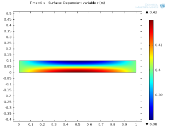
(a) Initial distribution of reds

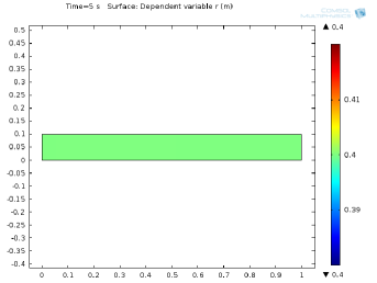
(b) Distribution of reds at time $T=5$

Figure 1: Solution to system (5) with no cohesion and aversion.

In this example we do not observe the formation of directional lanes as the solutions return to the equilibrium state quickly.

IV-2 Example 2

Let $\gamma_{0}=0.001$, $\gamma_{1}=0.5$, $\gamma_{2}=0.4$, $\alpha=0.2$ and $h=0.1$, i.e. $\gamma_{1}-\gamma_{2}=\mathcal{O}(h)$. As initial values we choose again (12), i.e. small perturbations of an equilibrium state. Figure 2 shows the solution $r_{T}$ and $b_{T}$ to system (5) at time $T=5$.

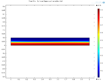
(a) Density of reds at time $T=5$

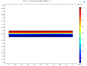
(b) Density of blues at time $T=5$

Figure 2: Solution to system (5) with cohesion and aversion.

In this example we observe lane formation. Since $\gamma_{1}>\gamma_{2}$ individuals have a tendency to step to the right. This tendency can also be observed in the formation of the directional lanes. The red individuals concentrate on the bottom of the corridor, whereas the blue individuals move to the top.

V Conclusion and outlook to further applications

In this paper, we have presented a symbolic approach to derive the mean-field PDEs from lattice-based models. We demonstrated the methods in terms of one example in pedestrian dynamics, but the algorithm may also be applied to other examples. In [1] different motility mechanisms on regular lattices are introduced, which result in nonlinear diffusion equations with different diffusivities. The authors considered various motilities based on attraction or repulsion, i.e. the transition rate to move away from a neighbouring individual increases or decreases respectively. For example, in a minimal model the transition rate is given by

$$\mathcal{T}^{i\rightarrow i+1}=(1-c_{i+1})(1-\alpha c_{i-1}),$$

where $c_{i}$ again denotes the probability that the lattice site $x_{i}$ is occupied. Hence the transition to move from $x_{i}$ to $x_{i+1}$ is reduced if the neighbouring site $x_{i-1}$ is occupied. This phenomenon is known as adhesion and results in a nonlinear diffusion model for the cell density $c=c(x,t)$ of the form

$$\partial_{t}c=\partial_{x}(D(c)\partial_{x}c),$$

with a diffusivity of the form $D(c)=3\alpha(c-\frac{2}{3})^{2}+1-\frac{4}{3}\alpha$, see [28]. Again in [1] several other transition rates were proposed, which lead to different nonlinear diffusitivies, see Table 1 there. Using our implementation, the entries in that table can be generated automatically. For example, we have tried one of their most complicated models [1, Equation (13)], which combines contact-forming or contact-breaking interactions with contact-maintaining interactions. Our implementation correctly derives the diffusivity given in [1, Equation (14)], where we have chosen the two-dimensional square lattice with Moore interacting neighborhoods.

References

- [1] A. E. Fernando, K. A. Landman, and M. J. Simpson, “Nonlinear diffusion and exclusion processes with contact interactions,” Physical Review E, vol. 81, no. 011903, 2010.
- [2] M. J. Simpson, R. E. Baker, and S. W. McCue, “Models of collective cell spreading with variable cell aspect ratio: a motivation for degenerate diffusion models,” Physical Review E, vol. 83, no. 021901, 2011.
- [3] M. Burger, M. Di Francesco, J.-F. Pietschmann, and B. Schlake, “Nonlinear cross-diffusion with size exclusion,” SIAM Journal on Mathematical Analysis, vol. 42, no. 6, pp. 2842–2871, 2010.
- [4] M. Burger, B. Schlake, and M. Wolfram, “Nonlinear Poisson–Nernst–Planck equations for ion flux through confined geometries,” Nonlinearity, vol. 25, no. 961, 2012.
- [5] M. J. Lighthill and G. B. Whitham, “On kinematic waves. II. a theory of traffic flow on long crowded roads,” in Proceedings of the Royal Society of London A: Mathematical, Physical and Engineering Sciences, vol. 229, no. 1178. The Royal Society, 1955, pp. 317–345.
- [6] M. Burger, P. A. Markowich, and J.-F. Pietschmann, “Continuous limit of a crowd motion and herding model: analysis and numerical simulations,” Kinetic and Related Models, vol. 4, no. 4, pp. 1025–1047, 2011.
- [7] M. Burger, M. D. Francesco, P. A. Markowich, and M.-T. Wolfram, “Mean field games with nonlinear mobilities in pedestrian dynamics,” Discrete and Continuous Dynamical Systems - Series B, vol. 19, no. 5, pp. 1311–1333, 2014.
- [8] M. J. Simpson, A. Merrifield, K. A. Landman, and B. D. Hughes, “Simulating invasion with cellular automata: connecting cell-scale and population-scale properties,” Physical Review E, vol. 76, no. 021918, 2007.
- [9] V. J. Blue and J. L. Adler, “Cellular automata microsimulation for modeling bi-directional pedestrian walkways,” Transportation Research Part B: Methodological, vol. 35, no. 3, pp. 293–312, 2001.
- [10] C. Burstedde, K. Klauck, A. Schadschneider, and J. Zittartz, “Simulation of pedestrian dynamics using a two-dimensional cellular automaton,” Physica A: Statistical Mechanics and its Applications, vol. 295, no. 3, pp. 507–525, 2001.
- [11] C. Cercignani, Rarefied gas dynamics: from basic concepts to actual calculations. Cambridge University Press, 2000.
- [12] C. Kipnis and C. Landim, Scaling limits of interacting particle systems. Springer Science & Business Media, 2013, vol. 320.
- [13] A. Stevens, “The derivation of chemotaxis equations as limit dynamics of moderately interacting stochastic many-particle systems,” SIAM Journal on Applied Mathematics, vol. 61, no. 1, pp. 183–212, 2000.
- [14] K. Oelschläger, “On the derivation of reaction-diffusion equations as limit dynamics of systems of moderately interacting stochastic processes,” Probability Theory and Related Fields, vol. 82, no. 4, pp. 565–586, 1989.
- [15] C. J. Penington, B. D. Hughes, and K. A. Landman, “Building macroscale models from microscale probabilistic models: a general probabilistic approach for nonlinear diffusion and multispecies phenomena,” Physical Review E, vol. 84, no. 4, p. 041120, 2011.
- [16] R. H. Risch, “The problem of integration in finite terms,” Transactions of the American Mathematical Society, vol. 139, pp. 167–189, 1969.
- [17] M. Bronstein, Symbolic Integration I. Berlin, Heidelberg, New York: Springer Verlag, 1997.
- [18] J. F. Ritt, Differential Algebra. New York: American Mathematical Society, 1950.
- [19] E. Kolchin, Differential algebra and algebraic groups. New York-London: Academic Press, 1973.
- [20] G. H. Campbell, “Symbolic integration of expressions involving unspecified functions,” SIGSAM Bulletin, vol. 22, no. 1, pp. 25–27, 1988.
- [21] A. H. Bilge, “A REDUCE program for the integration of differential polynomials,” Computer Physics Communications, vol. 71, pp. 263–268, 1992.
- [22] M. Rosenkranz and G. Regensburger, “Integro-differential polynomials and operators,” in Proceedings of the International Symposium on Symbolic and Algebraic Computation (ISSAC). New York, USA: ACM, 2008, pp. 261–268.
- [23] M. Rosenkranz, G. Regensburger, L. Tec, and B. Buchberger, “Symbolic analysis for boundary problems: From rewriting to parametrized Gröbner bases,” in Numerical and Symbolic Scientific Computing: Progress and Prospects, U. Langer and P. Paule, Eds. Vienna: Springer Wien New York, 2012, pp. 273–331.
- [24] C. G. Raab, “Definite Integration in Differential Fields,” Ph.D. dissertation, University of Linz, 2012.
- [25] ——, “Integration of unspecified functions and families of iterated integrals,” in Proceedings of the International Symposium on Symbolic and Algebraic Computation (ISSAC). New York, USA: ACM, 2013, pp. 323–330.
- [26] F. Boulier, F. Lemaire, G. Regensburger, and M. Rosenkranz, “On the integration of differential fractions,” in Proceedings of the International Symposium on Symbolic and Algebraic Computation (ISSAC). New York, USA: ACM, 2013, pp. 101–108.
- [27] F. Boulier, A. Korporal, F. Lemaire, W. Perruquetti, A. Poteaux, and R. Ushirobira, “An algorithm for converting nonlinear differential equations to integral equations with an application to parameter estimation from noisy data.” in Proceedings of CASC 2014 (eds. V.P. Gerdt, W. Koepf, W.M. Seiler, E.H. Vorozhtsov), LNCS 8660, Springer International Publishing, 2014, pp. 28–43.
- [28] K. Anguige and C. Schmeiser, “A one-dimensional model of cell diffusion and aggregation, incorporating volume filling and cell-to-cell adhesion,” Journal of Mathematical Biology, vol. 58, no. 3, pp. 395–427, 2009.