Tell and Predict: Kernel Classifier Prediction for Unseen Visual Classes from Unstructured Text Descriptions

Abstract

In this paper we propose a framework for predicting kernelized classifiers in the visual domain for categories with no training images where the knowledge comes from textual description about these categories. Through our optimization framework, the proposed approach is capable of embedding the class-level knowledge from the text domain as kernel classifiers in the visual domain. We also proposed a distributional semantic kernel between text descriptions which is shown to be effective in our setting. The proposed framework is not restricted to textual descriptions, and can also be applied to other forms knowledge representations. Our approach was applied for the challenging task of zero-shot learning of fine-grained categories from text descriptions of these categories.

1 Introduction

We propose a framework to model kernelized classifier prediction in the visual domain for categories with no training images, where the knowledge about these categories comes from a secondary domain. The side information can be in the form of textual, parse trees, grammar, visual representations, concepts in the ontologies, or any form; see Fig 1. Our work focuses on the unstructured text setting. We denote the side information as “privileged” information, borrowing the notion from  [Vapnik and Vashist, 2009].

Our framework is an instance of the concept of Zero Shot Learning (ZSL)[Larochelle et al., 2008], aiming at transferring knowledge from seen classes to novel (unseen) classes. Most zero-shot learning applications in practice use symbolic or numeric visual attribute vectors [Lampert et al., 2014, Lampert et al., 2009]. In contrast, recent works investigated other forms of descriptions, e.g. user provided feedback [Wah and Belongie, 2013], textual descriptions [Elhoseiny et al., 2013]. It is common in zero-shot learning to introduce an intermediate layer that facilitates knowledge sharing between seen classes, hence the transfer of knowledge to unseen classes. Typically, visual attributes are being used for that purpose, since they provide a human-understandable representation, which enables specifying new categories [Lampert et al., 2014, Lampert et al., 2009, Farhadi et al., 2009, Palatucci et al., 2009, Akata et al., 2013, Li et al., 2014]. A fundamental question in attribute-based ZSL models is how to define attributes that are visually discriminative and human understandable. Researchers has explored learning attributes from text sources, e.g.  [Rohrbach, 2014, Rohrbach et al., 2013, Rohrbach et al., 2010, Berg et al., 2010]. Other works have explored interactive methodologies to learning visual attribute that are human understandable, e.g.  [Parikh and Grauman, 2011].

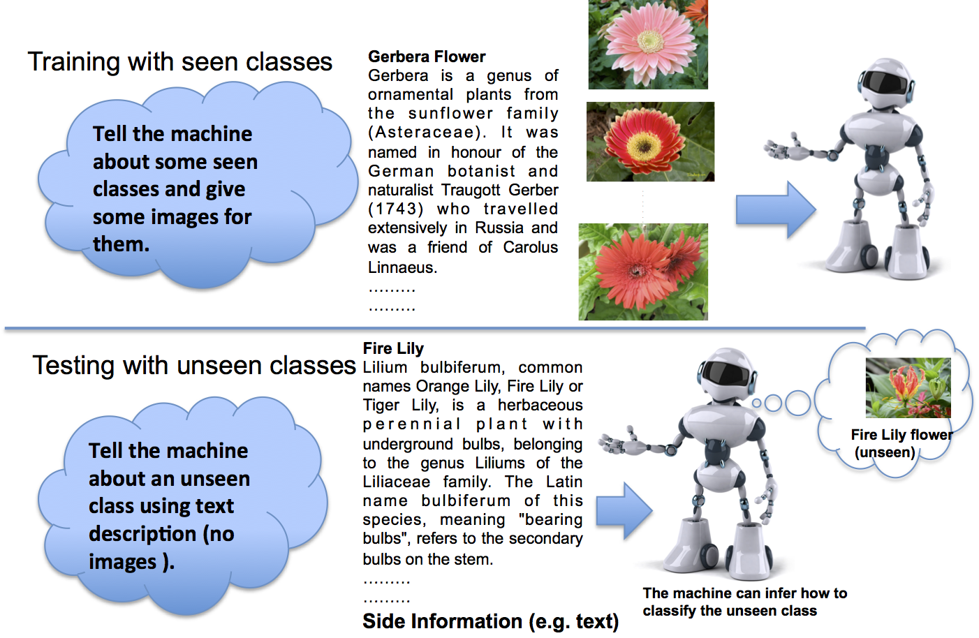
Figure 1: Our setting where machine can predict unseen class from pure unstructured text

There are several differences between our proposed framework and the state-of-the-art zero-shot learning approaches. We are not restricted to use attributes as the interface to specify new classes. We can use any “privileged” information available for each category. In particular in this paper we focus on the case of textual description of categories as the secondary domain. This difference is reflected in our zero-shot classification architecture. We learn a domain transfer model between the visual domain and the privileged information domain. This facilitates predicting explicit visual classifiers for novel unseen categories given their privileged information. The difference in architecture becomes clear if we consider, for the sake of argument, attributes as the secondary domain in our framework, although this is not the focus of the paper. In that case we do not need explicit attribute classifiers to be learned as an intermediate layer as typically done in attribute-based ZSL e.g.  [Lampert et al., 2009, Farhadi et al., 2009, Palatucci et al., 2009], instead the visual classifier are directly learned from the attribute labels. The need to learn an intermediate attribute classifier layer in most attribute-based zero-shot learning approaches dictates using strongly annotated data, where each image comes with attribute annotation, e.g. CU-Birds dataset [Welinder et al., 2010]. In contrast, we do not need image-annotation pairs, and privileged information is only assumed at the category level; hence we denote our approach weakly supervised. This also directly facilitates using continuous attributes in our case, and does not assume independent between attributes.

Another fundamental difference in our case is that we predict explicit kernel classifier in the form defined in the representer theorem [Schölkopf et al., 2001], from privileged information. Explicit classifier prediction means that the output of our framework is classifier parameters for any new category given text description, which can applied to any test image to predict its class. Predicting classifier in kernelized form opens the door for using any kind of side information about classes, as long as kernels can be defined on them. The image features also do not need to be in a vectorized format. Kernelized classifiers also facilitates combining different types of features through a multi-kernel learning (MKL) paradigm, where the fusion of different features can be effectively achieved.

We can summarize the features of our proposed framework, hence the contribution as follows: 1) Our framework explicitly predicts classifiers; 2) The predicted classifiers are kernelized; 3) The framework facilitates any type of “side” information to be used; 4) The approach requires the side information at the class level, not at the image level, hence, it needs only weak annotation. 5) We propose a distributional semantic kernel between text description of visual classes that we show its value in the experiments. The structure of the paper is as follows. Sec 2 describes the relation to existing literature. Sec 3 and  4 explains the learning setting and our formulation. Sec 5 presents the proposed distributional semantic kernel for text descriptions. Sec 6 shows our experimental results.

2 Related Work

We already discussed the relation to the zero-shot learning literature in the Introduction section. In this section, we focus on the relations to other volumes of literature.

There has been increasing interest recently in the intersection between Language and Computer Vision. Most of the work on this area is focused on generating textual description from images [Farhadi et al., 2010, Kulkarni et al., 2011, Ordonez et al., 2011, Yang et al., 2011, Mitchell et al., 2012]. In contrast, we focus on generating visual classifiers from textual description or other side information at the category level.

There are few recent works that involved unannotated text to improve visual classification or achieve zero-shot learning. In [Frome et al., 2013, Norouzi et al., 2014] and  [Socher et al., 2013], word embedding language models (e.g.  [Mikolov et al., 2013b]) was adopted to represent class names as vectors. Their framework is based on mapping images into the learned language mode then perform classification in that space. In contrast, our framework maps the text information to a classifier in the visual domain, i.e. the apposite direction of their approach. There are several advantages in mapping textual knowledge into the visual domain. To perform ZSL, approaches such as [Norouzi et al., 2014, Frome et al., 2013, Socher et al., 2013] only embed new classes by their category names. This has clear limitations when dealing with fine-grained categories (such as different bird species). Most of fine-grained category names does not exist in current semantic models. Even if they exist, they will end up close to each other in the learned language models since they typically share similar contexts. This limits the discriminative power of such language models. In fact our baseline experiment using these models performed as low as random when applied to fine-grained category; described in Sec 6.4. Moreover, our framework directly can use large text description of novel categories. In contrast to [Norouzi et al., 2014, Frome et al., 2013, Socher et al., 2013] which required a vectorized representation of images, our framework facilitates non-linear classification using kernels.

In [Elhoseiny et al., 2013], an approach was proposed to predict linear classifiers from textual description, based on a domain transfer optimization method proposed in [Kulis et al., 2011]. Although both of these works are kernelized, a close look reveals that kernelization was mainly used to reduce the size of the domain transfer matrix and the computational cost. The resulting predicted classifier in [Elhoseiny et al., 2013] is still a linear classifier. In contrast, our proposed formulation predicts kernelized visual classifiers directly from the domain transfer optimization, which is a more general case. This directly facilitates using classifiers that fused multiple visual cues such as Multiple Kernel Learning (MKL).

3 Problem Definition

We consider a zero-shot multi-class classification setting on domain $\mathcal{X}$ as follows. At training, besides the data points from $\mathcal{X}$ and the class labels, each class is associated with privileged information in a secondary domain $\mathcal{E}$ in particular, however not limited to, a textual description. We assume that each class $y_{i}\in{Y}_{sc}$(training/seen labels), is associated with privileged information $e_{i}\in\mathcal{E}$. While, our formulation allows multiple pieces of privileged information per class (e.g. multiple class-level textual descriptions), we will use one per class for simplicity. Hence, we denote the training as $\mathcal{D}_{train}=\{{S}_{x}=\{({x}_{i},y_{i})\}_{N},{S}_{e}=\{y_{j},{e}_{j}\}_{N_{sc}}\}$, where ${x}_{i}\in\mathcal{X}$, $y_{i}\in{Y}_{sc}$, $y_{j}\in{Y}_{sc}$, and $N_{sc}$ and $N$ are the number of the seen classes and the training examples/images respectively. We assume that each of the domains is equipped with a kernel function corresponding to a reproducing kernel Hilbert space (RKHS). Let us denote the kernel for $\mathcal{X}$ by $k(\cdot,\cdot)$ and the kernel for $\mathcal{E}$ by $g(\cdot,\cdot)$. At the zero-shot time, only the privileged information ${e}_{z^{*}}$ is available for each novel unseen class $z^{*}$; see Fig 1.

The common approach for multi-class classification is to learn a classifier for each class against the remaining classes (i.e., one-vs-all). According to the generalized representer theorem [Schölkopf et al., 2001], a minimizer of a regularized empirical risk function over an RKHS could be represented as a linear combination of kernels, evaluated on the training set. Adopting the representer theorem on classification risk function, we define a kernel-classifier of class $y$ as follows

$$f_{y}({x}^{*})=\sum_{i=1}^{N}\beta_{y}^{i}k({x}^{*},{x}_{i})+b={\boldsymbol{\beta}_{y}}^{\textsf{T}}\textbf{k}(x^{*}),$$ (1)

where ${x}^{*}\in\mathcal{X}$ is the test point, ${x}_{i}\in{S}_{x}$, $\textbf{k}(x^{*})=[k({x}^{*},{x}_{1}),\cdots,k({x}^{*},{x}_{N}),1]^{\textsf{T}},$ $\boldsymbol{\beta}_{y}=[\beta_{y}^{1}\cdots\beta_{y}^{N},b]^{\textsf{T}}$. Having learned $f_{y}({x}^{*})$ for each class $y$ (for example using SVM classifier), the class label of the test point ${x}^{*}$ can be predicted as

$$y^{*}=\arg\max_{y}f_{y}(\mathbf{x}^{*})$$ (2)

It is clear that $f_{y}(\mathbf{x}^{*})$ could be learned for all classes with training data $y\in{Y}_{sc}={y_{{}_{1}}\cdots y_{{}_{N_{sc}}}}$, since there are examples ${S}_{x}$ for the seen classes; we denote the kernel-classifier parameters of the seen classes as $\mathcal{B}_{sc}=\{\boldsymbol{\beta}_{y}\}_{N_{sc}},\forall y\in Y_{sc}$. However, it is not obvious how to predict $f_{z^{*}}(\mathbf{x}^{*})$ for a new unseen class $z^{*}\in{Y}_{us}={z_{{}_{1}}\cdots z_{{}_{N_{us}}}}$. Our main notion is to use the privileged information ${e}_{z^{*}}\in\mathcal{E}$, associated with unseen class $z^{*}$, and the training data $\mathcal{D}_{train}$ to directly predict the unseen kernel-classifier parameters. Hence, the classifier of $z^{*}$ is a function of $e_{k^{*}}$ and $\mathcal{D}_{train}$; i.e.

$$f_{z^{*}}(\mathbf{x}^{*})=\boldsymbol{\beta}({e}_{z^{*}},\mathcal{D}_{train})^{\textsf{T}}\cdot\textbf{k}(x^{*}),$$ (3)

$f_{z^{*}}(\mathbf{x}^{*})$ could be used to classify new points that belong to an unseen class as follows: 1) one-vs-all setting $f_{z^{*}}(\mathbf{x}^{*})\gtrless 0$ ; or 2) in a Multi-class prediction as in Eq  2.

4 Approach

Prediction of $\boldsymbol{\beta}({e}_{z^{*}},\mathcal{D}_{train})$, which we denote as $\boldsymbol{\beta}({e}_{z^{*}})$ for simplicity, is decomposed into training (domain transfer) and prediction phases.

4.1 Domain Transfer

During training, we firstly learn $\mathcal{B}_{sc}$ as SVM-kernel classifiers based on $\mathcal{S}_{x}$. Then, we learn a domain transfer function to transfer the privileged information ${e}\in\mathcal{E}$ to kernel-classifier parameters $\boldsymbol{\beta}\in\mathbb{R}^{N+1}$ in $\mathcal{X}$ domain. We call this function $\boldsymbol{\beta}_{DA}(e)$, which has the form of ${\textbf{T}}^{\textsf{T}}{\textbf{g}(e)}$, where $\textbf{g}(e)=[g({e},{e}_{1})\cdots g({e},{e}_{N_{sc}})]^{\textsf{T}}$; T is an $N_{sc}\times{N+1}$ matrix, which transforms ${e}$ to kernel classifier parameters for the class ${e}$ represents.

We aim to learn T, such that $\textbf{g}(e)^{\textsf{T}}{\textbf{T}}\textbf{k}(x)>l$ if ${e}$ and $x$ correspond to the same class, $\textbf{g}(e)^{\textsf{T}}{\textbf{T}}\textbf{k}(x)<u$ otherwise. Here $l$ controls similarity lower-bound if $e$ and $x$ correspond to same class, and $u$ controls similarity upper-bound if $e$ and $x$ belong to different classes. In our setting, the term ${\textbf{T}}^{\textsf{T}}{\textbf{g}(e_{i})}$ should act as a classifier parameter for class $i$ of the training data. Therefore, we introduce penalization constraints to our minimization function if ${\textbf{T}}^{\textsf{T}}{\textbf{g}(e_{i})}$ is distant from $\boldsymbol{\beta}_{i}\in\mathcal{B}_{sc}$, where ${e}_{i}$ corresponds to the class that $\boldsymbol{\beta}_{i}$ classifies. Inspired by domain adaptation optimization methods (e.g. [Kulis et al., 2011]), we model our domain transfer function as follows

$$\begin{split}{\textbf{T}^{*}}=\arg\min_{{\textbf{T}}}L({\textbf{T}})=[&\frac{1}{2}r({\textbf{T}})+\lambda_{1}\sum_{k}c_{k}(\mathbf{G}{\textbf{T}}\mathbf{K})+\\ &\lambda_{2}\sum_{i=1}^{N_{sc}}{\|\boldsymbol{\beta}_{i}-{\textbf{T}}^{\textsf{T}}{\textbf{g}(e_{i})}\|^{2}}\end{split}$$ (4)

where, $\mathbf{G}$ is an $N_{sc}\times N_{sc}$ symmetric matrix, such that both the $i^{th}$ row and the $i^{th}$ column are equal to $\textbf{g}(e_{i})$, $e_{i}\in\mathcal{S}_{e}$; $\mathbf{K}$ is an $N+1\times N$ matrix, such that the $i^{th}$ column is equal to $\textbf{k}(x_{i})$, $x_{i}\in\mathcal{S}_{x}$. $c_{k}$’s are loss functions over the constraints defined as $c_{k}(\mathbf{G}{\textbf{T}}\mathbf{K}))=(max(0,(l-\textbf{1}_{i}^{\textsf{T}}\mathbf{G}{\textbf{T}}\mathbf{K}\textbf{1}_{j})))^{2}$ for same class pairs of index $i$ and $j$, or $=r\cdot(max(0,(\textbf{1}_{i}^{\textsf{T}}\mathbf{G}{\textbf{T}}\mathbf{K}\textbf{1}_{j}-u)))^{2}$ otherwise, where $\textbf{1}_{i}$ is an $N_{sc}\times 1$ vector with all zeros except at index $i$, $\textbf{1}_{j}$ is an $N\times 1$ vector with all zeros except at index $j$. This leads to $c_{k}(\mathbf{G}{\textbf{T}}\mathbf{K})=max(0,(l-\textbf{g}(e_{i})^{\textsf{T}}{\textbf{T}}\textbf{k}(x_{j})))^{2}$ for same class pairs of index $i$ and $j$, or $=r\cdot(max(0,(\textbf{g}(e_{i})^{\textsf{T}}{\textbf{T}}\textbf{k}(x_{j})-u)))^{2}$ otherwise, where $u>l$, $r=\frac{nd}{ns}$ such that $nd$ and $ns$ are the number of pairs $(i,j)$ of different classes and similar pairs respectively. Finally, we used a Frobenius norm regularizer for $r({\textbf{T}})$.

The objective function in Eq  4 controls the involvement of the constraints $c_{k}$ by the term multiplied by $\lambda_{1}$, which controls its importance; we call it $C_{l,u}({\textbf{T}})$. While, the trained classifiers penalty is captured by the term multiplied by $\lambda_{2}$; we call it $C_{\beta}({\textbf{T}})$. One important observation on $C_{\beta}({\textbf{T}})$ is that it reaches zero when ${\textbf{T}}=\mathbf{G}^{-1}\textbf{B}^{\mathsf{T}}$, where $\textbf{B}=[\boldsymbol{\beta}_{1}\cdots\boldsymbol{\beta}_{N_{sc}}]$, since it could be rewritten as $C_{\beta}({\textbf{T}})=\|\textbf{B}^{\mathsf{T}}-\mathbf{G}{\textbf{T}}\|_{F}^{2}$.

One approach to minimize $L({\textbf{T}})$ is gradient-based optimization using a quasi-Newton optimizer. Our gradient derivation of $L({\textbf{T}})$ leads to the following form

$$\frac{\delta L({\textbf{T}})}{\delta{\textbf{T}}}={\textbf{T}}+\lambda_{1}\cdot\sum_{i,j}{\mathbf{g}(e_{i})}{\mathbf{k}(x_{j})}^{\mathsf{T}}v_{ij}+r\cdot\lambda_{2}\cdot(\mathbf{G}^{2}{\textbf{T}}-\mathbf{G}\textbf{B})$$ (5)

where $v_{ij}=-2\cdot max(0,(l-\textbf{g}(e_{i})^{\mathsf{T}}{\textbf{T}}\textbf{k}(x_{j})))$ if $i$ and $j$ correspond to the same class, $2\cdot max(0,(\textbf{g}(e_{i})^{\mathsf{T}}{\textbf{T}}\textbf{k}(x_{j})-u)$ otherwise. Another approach to minimize $L({\textbf{T}})$ is through alternating projection using Bregman algorithm [Censor and Zenios, 1997], in which T is updated with respect to a single constraint every iteration.

4.2 Classifier Prediction

We propose two ways to predict the kernel-classifier. (1) Domain Transfer (DT) Prediction, (2) One-class-SVM adjusted DT Prediction.

Domain Transfer (DT) Prediction: Construction of an unseen category is directly computed from our domain transfer model as follows

$$\centering\begin{split}\tilde{\boldsymbol{\beta}}_{DT}(\mathbf{e}_{z^{*}})=\mathbf{{\textbf{T}^{*}}}^{\textsf{T}}\mathbf{g}(e_{z^{*}})\end{split}\@add@centering$$ (6)

One-class-SVM adjusted DT (SVM-DT) Prediction: In order to increase separability against seen classes, we adopted the inverse of the idea of the one class kernel-svm, whose main idea is to build a confidence function that takes only positive examples of the class. Our setting is the opposite scenario; seen examples are negative examples of the unseen class. In order introduce our proposed adjustment method, we start by presenting the one-class SVM objective function. The Lagrangian dual of the one-class SVM [Evangelista et al., 2007] can be written as

$$\begin{split}{\boldsymbol{\beta}}^{*}_{+}=&\underset{\boldsymbol{\beta}}{\operatorname{argmin}}\big{[}\boldsymbol{\beta}^{\textsf{T}}\mathbf{K^{{}^{\prime}}}\boldsymbol{\beta}-\boldsymbol{\beta}^{T}\mathbf{a}\big{]}\\ &s.t.:\boldsymbol{\beta}^{T}\mathbf{1}=1,0\leq\boldsymbol{\beta}_{i}\leq C;i=1\cdots N\\ \end{split}$$ (7)

where $\mathbf{K^{{}^{\prime}}}$ is an $N\times N$ matrix, $\mathbf{K^{{}^{\prime}}}(i,j)=k({x}_{i},{x}_{j})$, $\forall{x}_{i},{x}_{j}\in\mathcal{S}_{x}$ (i.e. in the training data), a is an $N\times 1$ vector, $\textbf{a}_{i}=k({x}_{i},{x}_{i})$, $C$ is a hyper-parameter . It is straightforward to see that, if $\beta$ is aimed to be a negative decision function instead, the objective function becomes in the form

$$\begin{split}{\boldsymbol{\beta}}^{*}_{-}=&\underset{\boldsymbol{\beta}}{\operatorname{argmin}}\big{[}\boldsymbol{\beta}^{\textsf{T}}\mathbf{K^{{}^{\prime}}}\boldsymbol{\beta}+\boldsymbol{\beta}^{T}\mathbf{a}\big{]}\\ &s.t.:\boldsymbol{\beta}^{T}\mathbf{1}=-1,-C\leq\boldsymbol{\beta}_{i}\leq 0;i=1\cdots N\\ \end{split}$$ (8)

While ${\boldsymbol{\beta}}^{*}_{-}=-{\boldsymbol{\beta}}^{*}_{+}$, the objective function in Eq 8 of the one-negative class SVM inspires us with the idea to adjust the kernel-classifier parameters to increase separability of the unseen kernel-classifier against the points of the seen classes, which leads to the following objective function

$$\begin{split}\hat{\boldsymbol{\beta}}(\mathbf{e}_{z^{*}})=&\underset{\boldsymbol{\beta}}{\operatorname{argmin}}\big{[}\boldsymbol{\beta}^{\textsf{T}}\mathbf{K^{{}^{\prime}}}\boldsymbol{\beta}-\zeta\hat{\boldsymbol{\beta}}_{DT}(\mathbf{e}_{z^{*}})^{\textsf{T}}\mathbf{K^{{}^{\prime}}}\boldsymbol{\beta}+\boldsymbol{\beta}^{T}\mathbf{a}\big{]}\\ &s.t.:\boldsymbol{\beta}^{T}\mathbf{1}=-1,{\hat{\boldsymbol{\beta}}_{DT}}^{\mathsf{T}}\mathbf{K^{{}^{\prime}}}\boldsymbol{\beta}>l,-C\leq\boldsymbol{\beta}_{i}\leq 0;\forall i\\ &C,\zeta,l\text{: hyper-parameters},\\ \end{split}$$ (9)

where $\hat{\boldsymbol{\beta}}_{DT}$ is the first $N$ elements in $\tilde{\boldsymbol{\beta}}_{DT}\in\mathbb{R}^{N+1}$, $\mathbf{1}$ is an $N\times 1$ vector of ones. The objective function, in Eq 9, pushes the classifier of the unseen class to be highly correlated with the domain transfer prediction of the kernel classifier, while putting the points of the seen classes as negative examples. It is not hard to see that Eq 9 is a quadratic program in $\mathbf{\beta}$, which could be solved using any quadratic solver; we used IBM CPLEX. It is worth to mention that, the approach in [Elhoseiny et al., 2013] predicts linear classifiers by solving an optimization problem of size $N+d_{X}+1$ variables ($d_{X}+1$ linear-classifier parameters and $N$ slack variables); a similar limitation can be found in [Frome et al., 2013, Socher et al., 2013]. In contrast, our objective function in Eq 9 solves a quadratic program of only $N$ variables, and predicts a kernel-classifier instead, with fewer parameters. Hence, if very high-dimensional features are used, they will not affect our optimization complexity.

5 Distributional Semantic (DS) Kernel for text descriptions

When $\mathcal{E}$ domain is the space of text descriptions, we propose a distributional semantic kernel $g(\cdot,\cdot)=g_{DS}(\cdot,\cdot)$ to define the similarity between two text descriptions . We start by distributional semantic models by [Mikolov et al., 2013c, Mikolov et al., 2013a] to represent the semantic manifold $\mathcal{M}_{s}$, and a function $vec(\cdot)$ that maps a word to a $K\times 1$ vector in $\mathcal{M}_{s}$. The main assumption behind this class of distributional semantic model is that similar words share similar context. Mathematically speaking, these models learn a vector for each word $w_{n}$, such that $p(w_{n}|(w_{n-L},w_{n-L+1},\cdots,w_{n+L-1},w_{n+L})$ is maximized over the training corpus, where $2\times L$ is the context window size. Hence similarity between $vec(w_{i})$ and $vec(w_{j})$ is high if they co-occurred a lot in context of size $2\times L$ in the training text-corpus. We normalize all the word vectors to length $1$ under L2 norm, i.e., $\|vec(\cdot)\|^{2}=1$.

Let us assume a text description ${D}$ that we represent by a set of triplets ${D}=\{(w_{l},f_{l},vec(w_{l})),l=1\cdots M\}$, where $w_{l}$ is a word that occurs in ${D}$ with frequency $f_{l}$ and its corresponding word vector is $vec(w_{l})$ in $\mathcal{M}_{s}$. We drop the stop words from ${D}$. We define $\textbf{F}=[f_{1},\cdots,f_{M}]^{\textsf{T}}$ and $\textbf{V}=[vec(w_{1}),\cdots,vec(w_{M})]^{\textsf{T}}$, where F is an $M\times 1$ vector of term frequencies and V is an $M\times K$ matrix of the corresponding term vectors.

Given two text descriptions ${D}_{i}$ and ${D}_{j}$ which contains $M_{1}$ and $M_{2}$ terms respectively. We compute $\textbf{F}_{i}$ ($M_{i}\times 1$) and $\textbf{V}_{i}$ ($M_{i}\times K$) for ${D}_{i}$ and $\textbf{F}_{j}$ ($M_{j}\times 1$) and $\textbf{V}_{j}$ ($M_{j}\times K$) for ${D}_{j}$. Finally $g_{DS}({D}_{i},{D}_{j})$ is defined as

$$g_{DS}({D}_{i},{D}_{j})=\textbf{F}_{i}^{\textsf{T}}\textbf{V}_{i}\textbf{V}_{j}^{\textsf{T}}\textbf{F}_{j}$$ (10)

One advantage of this similarity measure is that it captures semantically related terms. It is not hard to see that the standard Term Frequency (TF) similarity could be thought as a special case of this kernel where $vec(w_{l})^{\mathsf{T}}vec(w_{m})=1$ if $w_{l}=w_{m}$, 0 otherwise, i.e., different terms are orthogonal. However, in our case the word vectors are learnt through a distributional semantic model which makes semantically related terms have higher dot product ($vec(w_{l})^{\mathsf{T}}vec(w_{m})$).

6 Experiments

6.1 Datasets and Evaluation Methodology

We validated our approach in a fine-grained setting using two datasets: 1) The UCSD-Birds dataset [Welinder et al., 2010], which consists of 6033 images of 200 classes. 2) The Oxford-Flower dataset [Nilsback and Zisserman, 2008], which consists of 8189 images of 102 flower categories. Both datasets were amended with class-level text descriptions extracted from different encyclopedias which is the same descriptions used in [Elhoseiny et al., 2013]; see samples in the supplementary materials. We split the datasets to 80% of the classes for training and 20% of the classes for testing, with cross validations. We report multiple metrics while evaluating and comparing our approach to the baselines, detailed as follows

Multiclass Accuracy of Unseen classes (MAU): Under this metric, we aim to evaluate the performance of the unseen classifiers against each others. Firstly, the classifiers of all unseen categories are predicted. Then, an instance $x^{*}$ is classified to the class $z^{*}\in{Y}_{us}$ of maximum confidence for $x^{*}$ of the predicted classifiers; see Eq 2.

AUC: In order to measure the discriminative ability of our predicted one-vs-all classifier for each unseen class, against the seen classes, we report the area under the ROC curve. Since unseen class positive examples are few compared to negative examples, a large accuracy could be achieved even if all unseen points are incorrectly classified. Hence, AUC is a more consistent measure. In this metric, we use the predicted classifier of an unseen class as a binary separator against the seen classes. This measure is computed for each predicted unseen classifier and the average AUC is reported. This is the only measure addressed in [Elhoseiny et al., 2013] to evaluate the unseen classifiers, which is limiting in our opinion.

$|N_{sc}|\,$to $|N_{sc}+1|\,$Recall: Under this metric, we aim to check how the learned classifiers of the seen classes confuse the predicted classifiers, when they are involved in a multi-class classification problem of $N_{sc}+1\,$classes. We use Eq 2 to predict label of an instance $x^{*}$, such that the unknown label $y^{*}\in{Y}_{sc}\cup l_{us}$, such that $l_{us}\,$is the label of the unseen class. We compute the recall under this setting. This metric is computed for each predicted unseen classifier and the average is reported.

6.2 Comparisons to Linear Classifier Prediction

We compared our proposed approach to [Elhoseiny et al., 2013], which predicts a linear classifier for zero-shot learning from textual descriptions ( $\mathcal{E}\,$space in our framework). The aspects of the comparison includes 1) whether the predicted kernelized classifier outperforms the predicted linear classifier 2) whether this behavior is consistent on multiple datasets. We performed the comparison on both Birds and Flower dataset. For these experiments, in our setting, domain $\mathcal{X}\,$is the visual domain and domain $\mathcal{E}\,$is the textual domain, i.e. , the goal is to predict classifiers from pure textual description. We used the same features on the visual domain and the textual domains as [Elhoseiny et al., 2013]. That is, for the visual domain, we used classeme features [Torresani et al., 2010], extracted from images of the Bird and the Flower datasets. Classeme is a 2569-dimensional features, which correspond to confidences of a set of one-vs-all classifiers, pre-trained on images from the web, as explained in [Torresani et al., 2010], not related to either the Bird nor the Flower datasets. The rationale behind using these features in [Elhoseiny et al., 2013] was that they offer a semantic representation. For the textual domain, we used the same textual feature extracted by [Elhoseiny et al., 2013]. In that work, tf-idf (Term-Frequency Inverted Document Frequency)[Salton and Buckley, 1988] features were extracted from the textual articles were used, followed by a CLSI [Zeimpekis and Gallopoulos, 2005] dimensionality reduction phase.

We denote our DT prediction and one class SVM adjust DT prediction approaches as DT-kernel and SVM-DT-kernel respectively. We compared against the linear classifier prediction by [Elhoseiny et al., 2013]. We also compared against the direct domain transfer [Kulis et al., 2011], which was applied as a baseline in [Elhoseiny et al., 2013] to predict linear classifiers. In our kernel approaches, we used Gaussian rbf-kernel as a similarity measure in $\mathcal{E}\,$and $\mathcal{X}\,$spaces (i.e. $k(d,d^{\prime})=exp(-\lambda||d-d^{\prime}||)$).

Table 1: Recall, MAU, and average AUC on three seen/unseen splits on Flower Dataset and a seen/unseen split on Birds dataset

	Recall-Flower	improvement	Recall-Birds	improvement
SVM-DT kernel-rbf	40.34% (+/- 1.2) %		44.05 %
Linear Classifier	31.33 (+/- 2.22)%	27.8 %	36.56 %	20.4 %

	MAU-Flower	improvement	MAU-Birds	improvement
SVM-DT kernel-rbf	9.1 (+/- 2.77) %		3.4 %
DT kernel-rbf	6.64 (+/- 4.1) %	37.93 %	2.95 %	15.25 %
Linear Classifier	5.93 (+/- 1.48)%	54.36 %	2.62 %	29.77 %
Domain Transfer	5.79 (+/- 2.59)%	58.46 %	2.47 %	37.65 %

	AUC-Flower	improvement	AUC-Birds	improvement
SVM-DT kernel-rbf	0.653 (+/- 0.009)		0.61
DT kernel-rbf	0.623 (+/- 0.01) %	4.7 %	0.57	7.02 %
Linear Classifier	0.658 (+/- 0.034)	- 0.7 %	0.62	-1.61%
Domain Transfer	0.644 (+/- 0.008)	1.28 %	0.56	8.93%

Recall metric : The recall of our approach is 44.05% for Birds and 40.34% for Flower, while it is 36.56% for Birds and 31.33% for Flower using [Elhoseiny et al., 2013]. This indicates that the predicted classifier is less confused by the classifiers of the seen compared with [Elhoseiny et al., 2013]; see table  1 (top part)

MAU metric: It is worth to mention that the multiclass accuracies for the trained seen classifiers are $51.3\%$ and $15.4\%$ using the classeme features on Flower dataset and Birds dataset, respectively. Table  1 (middle part) shows the average $MAU$ metric over three seen/unseen splits for Flower dataset and one split on Birds dataset, respectively. Furthermore, the relative improvements of our SVM-DT-kernel approach is reported against the baselines. On Flower dataset, it is interesting to see that our approach achieved $9.1\%$ MAU, $182\%$ improvement over the random guess performance, by predicting the unseen classifiers using just textual features as privileged information (i.e. $\mathcal{E}$ domain). We also achieved also $13.4\%$, $268\%$ the random guess performance, in one of the splits (the $9.1\%$ is the average over 3 seen/unseen splits). Similarity on Birds dataset, we achieved $3.4\%$ MAU from text features, $132\%$ the random guess performance (further improved to $224\%$ in next experiments).

AUC metric: Fig 2 (top part) shows the ROC curves for our approach on the best predicted unseen classes from the Flower dataset. Fig 2 (bottom part) shows the AUC for all the classes on Flower dataset (over three different splits). More results and figures are attached in the supplementary materials. Table 1 (bottom part) shows the average AUC on the two datasets, compared to the baselines.

Looking at table 1, we can notice that the proposed approach performs marginally similar to the baselines from AUC perspective. However, there is a clear improvement in MAU and Recall metrics. These results show the advantage of predicting classifiers in kernel space. Furthermore, the table shows that our SVM-DT-kernel approach outperforms our DT-kernel model. This indicates the advantage of the class separation, which is adjusted by the SVM-DT-kernel model. More details on the hyper-parameter selection are attached in the supplementary materials.

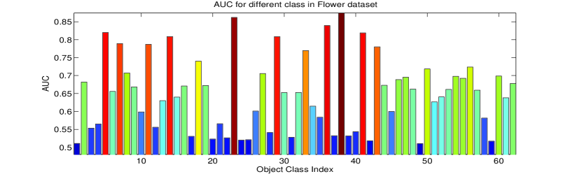
Figure 2: AUC of the 62 unseen classifiers the flower data-sets over three different splits (bottom part) and their Top 10 ROC-curves (top part)

6.3 Multiple Kernel Learning (MKL) Experiment

This experiment shows the added value of proposing a kernelized zero-shot learning approach. We conducted an experiment where the final kernel on the visual domain is produced by Multiple Kernel Learning [Gonen and Alpaydin, 2011]. For the visual domain, we extracted kernel descriptors for Birds dataset. Kernel descriptors provide a principled way to turn any pixel attribute to patch-level features, and are able to generate rich features from various recognition cues. We specifically used four types of kernels introduced by [Bo et al., 2010] as follows: Gradient Match Kernels that captures image variation based on predefined kernels on image gradients. Color Match Kernel that describes patch appearance using two kernels on top of RGB and normalized RGB for regular images and intensity for grey images. These kernels capture image variation and visual apperances. For modeling the local shape, Local Binary Pattern kernels have been applied.

We computed these kernel descriptors on local image patches with fixed size 16 x 16 sampled densely over a grid with step size 8 in a spatial pyramid setting with four layers. The dense features are vectorized using codebooks of size 1000. This process ended up with a 120,000 dimensional feature for each image (30,000 for each type). Having extracted the four types of descriptors, we compute an rbf kernel matrix for each type separately. We learn the bandwidth parameters for each rbf kernel by cross validation on the seen classes. Then, we generate a new kernel $k_{mkl}(d,d^{\prime})=\sum_{i=1}^{4}w_{i}k_{i}(d,d^{\prime})$, such that $w_{i}$ is a weight assigned to each kernel.

Table 2: MAU on a seen-unseen split-Birds Dataset (MKL)

	MAU	improvement
SVM-DT kernel-rbf (text)	4.10 %
Linear Classifier	2.74 %	49.6 %

We learn these weights by applying Bucak’s Multiple Kernel Learning algorithm [Bucak et al., 2010]. Then, we applied our approach where the MKL-kernel is used in the visual domain and rbf kernel on the text TFIDF features.

To compare our approach to [Elhoseiny et al., 2013] under this setting, we concatenated all kernel descriptors to end up with 120,000 dimensional feature vector in the visual domain. As highlighted in the approach Sec 4, the approach in [Elhoseiny et al., 2013] solves a quadratic program of $N+d_{X}+1\,$variables for each unseen class. Due to the large dimensionality of data ($d_{X}=120,000$), this is not tractable. To make this setting applicable, we reduced the dimensionality of the feature vector into $4000$ using PCA. This highlights the benefit of our approach since it does not depend on the dimensionality of the data. Table 2 shows MAU for our approach under this setting against [Elhoseiny et al., 2013]. The results show the benefits of having a kernel approach for zero shot learning where kernel methods are applied to improve the performance.

6.4 Multiple Representation Experiment and Distributional Semantic(DS) Kernel

The aim of this experiment is to show that our approach also work on different representations of text and visual domain. In this experiment, we extracted Convolutional Neureal Network(CNN) image features for the Visual domain. We used caffe [Jia et al., 2014] implementation of [Krizhevsky et al., 2012]. Then, we extracted the sixth activation feature of the CNN since we found it works the best on the standard classification setting. We found this consistent with the results of [Donahue et al., 2014] over different CNN layers. While using TFIDF feature of text description and CNN features for images, we achieved 2.65% for the linear version and 4.2% for the rbf kernel on both text and images. We further improved the performance to 5.35% by using our proposed Distributional Semantic (DS) kernel in the text domain and rbf kernel for images. In this DS experiment, we used the distributional semantic model by [Mikolov et al., 2013c] trained on GoogleNews corpus (100 billion words) resulting in a vocabulary of size 3 million words, and word vectors of $K=300$ dimensions. This experiment shows both the value of having a kernel version and also the value of the proposed kernel in our setting. We also applied the zero shot learning approach in [Norouzi et al., 2014] which performs worse in our settings; see Table 3.

Table 3: MAU on a seen-unseen split-Birds Dataset (CNN features, text description)

	MAU	improvement
SVM-DT kernel ($\mathcal{X}$-rbf, $\mathcal{E}$-DS kernel)	5.35 %
SVM-DT kernel ($\mathcal{X}$-rbf, $\mathcal{E}$-rbf on TFIDF)	4.20 %	27.3%
Linear Classifier (TFIDF text)	2.65 %	102.0%
[Norouzi et al., 2014]	2.3%	132.6%

6.5 Attributes Experiment

We emphasis that our main goal is not attribute prediction. However, it was interesting for us to see the behavior of our method where side information comes from attributes instead of text. In contrast to attribute-based models, which fully utilize attribute information to build attribute classifiers, our approach do not learn attribute classifiers. In this experiment, our method uses only the first moment of information of the attributes (i.e. the average attribute vector). We decided to compare to an attribute-based approach from this perspective. In particular, we applied the (DAP) attribute-based model [Lampert et al., 2014, Lampert et al., 2009], widely adopted in many applications (e.g., [Liu et al., 2013, Rohrbach et al., 2011]), to the Birds dataset. Details weak attribute representation in $\mathcal{E}$ space are attached in the supplementary materials due to space. For visual domain $\mathcal{X}$, we used classeme features in this experiment (like table 1 experiment)

Table 4: MAU on a seen-unseen split-Birds Dataset (Attributes)

	MAU	improvement
SVM-DT kernel-rbf	5.6 %
DT kernel-rbf	4.03 %	32.7 %
Lampert DAP	4.8 %	16.6 %

An interesting result is that our approach achieved $5.6\%$ MAU ($224\%$ the random guess performance); see Table  4. In contrast, we get $4.8\%$ multiclass accuracy using DAP approach [Lampert et al., 2014]. In this setting, we also measured the $N_{sc}$ to $N_{sc}+1$ average recall. We found the recall measure is $76.7\%$ for our SVM-DT-kernel, while it is $68.1\%$ on the DAP approach, which reflects better true positive rate (positive class is the unseen one). We find these results interesting, since we achieved it without learning any attribute classifiers, as in [Lampert et al., 2014]. When comparing the results of our approach using attributes (Table 4) vs. textual description (Table 1) as the privileged information used for prediction, it is clear that the attribute features gives better prediction. This support our hypothesis that the more meaningful the $\mathcal{E}\,$domain, the better the performance on $\mathcal{X}\,$domain.

7 Conclusion

We proposed an approach to predict kernel-classifiers of unseen categories textual description of them. We formulated the problem as domain transfer function from the privilege space $\mathcal{E}\,\,$to the visual classification space $\mathcal{X}$, while supporting kernels in both domains. We proposed a one-class SVM adjustment to our domain transfer function to improve the prediction. We validated the performance of our model by several experiments. We applied our approach using different privilege spaces (i.e. $\mathcal{E}\,\,$lives in a textual space or an attribute space). We showed the value of proposing a kernelized version by applying kernels generated by Multiple Kernel Learning (MKL) and achieved better results. We also compared our approach with state-of-the-art approaches and interesting findings have been reported.

References

- [Akata et al., 2013] Zeynep Akata, Florent Perronnin, Zaid Harchaoui, and Cordelia Schmid. 2013. Label-embedding for attribute-based classification. In CVPR.
- [Berg et al., 2010] Tamara L Berg, Alexander C Berg, and Jonathan Shih. 2010. Automatic attribute discovery and characterization from noisy web data. In ECCV.
- [Bo et al., 2010] L. Bo, X. Ren, and D. Fox. 2010. Kernel descriptors for visual recognition. In NIPS.
- [Bucak et al., 2010] Serhat Selcuk Bucak, Rong Jin, and Anil K. Jain. 2010. Multi-label multiple kernel learning by stochastic approximation: Application to visual object recognition. In NIPS.
- [Censor and Zenios, 1997] Y. Censor and S.A. Zenios. 1997. Parallel Optimization: Theory, Algorithms, and Applications. Oxford University Press, USA.
- [Donahue et al., 2014] Jeff Donahue, Yangqing Jia, Oriol Vinyals, Judy Hoffman, Ning Zhang, Eric Tzeng, and Trevor Darrell. 2014. Decaf: A deep convolutional activation feature for generic visual recognition. In ICML.
- [Elhoseiny et al., 2013] Mohammad Elhoseiny, Babak Saleh, and Ahmed Elgammal. 2013. Write a classifier: Zero shot learning using purely text descriptions. In ICCV.
- [Evangelista et al., 2007] Paul F. Evangelista, Mark J. Embrechts, and Boleslaw K. Szymanski. 2007. Some properties of the gaussian kernel for one class learning. In ICANN.
- [Farhadi et al., 2009] Ali Farhadi, Ian Endres, Derek Hoiem, and David A. Forsyth. 2009. Describing objects by their attributes. In CVPR.
- [Farhadi et al., 2010] Ali Farhadi, Mohsen Hejrati, Mohammad Amin Sadeghi, Peter Young, Cyrus Rashtchian, Julia Hockenmaier, and David Forsyth. 2010. Every picture tells a story: Generating sentences from images. In ECCV.
- [Frome et al., 2013] Andrea Frome, Gregory S. Corrado, Jonathon Shlens, Samy Bengio, Jeffrey Dean, Marc’Aurelio Ranzato, and Tomas Mikolov. 2013. Devise: A deep visual-semantic embedding model. In NIPS.
- [Gonen and Alpaydin, 2011] Mehmet Gonen and Ethem Alpaydin. 2011. Multiple kernel learning algorithms. JMLR.
- [Jia et al., 2014] Yangqing Jia, Evan Shelhamer, Jeff Donahue, Sergey Karayev, Jonathan Long, Ross Girshick, Sergio Guadarrama, and Trevor Darrell. 2014. Caffe: Convolutional architecture for fast feature embedding. In ACM Multimedia.
- [Krizhevsky et al., 2012] Alex Krizhevsky, Ilya Sutskever, and Geoffrey E Hinton. 2012. Imagenet classification with deep convolutional neural networks. In Advances in neural information processing systems (NIPS).
- [Kulis et al., 2011] B. Kulis, K. Saenko, and T. Darrell. 2011. What you saw is not what you get: Domain adaptation using asymmetric kernel transforms. In CVPR.
- [Kulkarni et al., 2011] Girish Kulkarni, Visruth Premraj, Sagnik Dhar, Siming Li, Yejin Choi, Alexander C Berg, and Tamara L Berg. 2011. Baby talk: Understanding and generating simple image descriptions. In CVPR.
- [Lampert et al., 2009] Christoph H. Lampert, Hannes Nickisch, and Stefan Harmeling. 2009. Learning to detect unseen object classes by betweenclass attribute transfer. In In CVPR.
- [Lampert et al., 2014] C.H. Lampert, H. Nickisch, and S. Harmeling. 2014. Attribute-based classification for zero-shot visual object categorization. TPAMI, 36(3):453–465, March.
- [Larochelle et al., 2008] Hugo Larochelle, Dumitru Erhan, and Yoshua Bengio. 2008. Zero-data learning of new tasks. In AAAI.
- [Li et al., 2014] Zhenyang Li, Efstratios Gavves, Thomas Mensink, and Cees GM Snoek. 2014. Attributes make sense on segmented objects. In ECCV.
- [Liu et al., 2013] Jingen Liu, Qian Yu, Omar Javed, Saad Ali, Amir Tamrakar, Ajay Divakaran, Hui Cheng, and Harpreet Sawhney. 2013. Video event recognition using concept attributes. In WACV.
- [Mikolov et al., 2013a] Tomas Mikolov, Kai Chen, Greg Corrado, and Jeffrey Dean. 2013a. Efficient estimation of word representations in vector space. ICLR.
- [Mikolov et al., 2013b] Tomas Mikolov, Ilya Sutskever, Kai Chen, Greg S Corrado, and Jeff Dean. 2013b. Distributed representations of words and phrases and their compositionality. In Advances in Neural Information Processing Systems, pages 3111–3119.
- [Mikolov et al., 2013c] Tomas Mikolov, Ilya Sutskever, Kai Chen, Greg S Corrado, and Jeff Dean. 2013c. Distributed representations of words and phrases and their compositionality. In Advances in Neural Information Processing Systems, pages 3111–3119.
- [Mitchell et al., 2012] Margaret Mitchell, Jesse Dodge, Amit Goyal, Kota Yamaguchi, Karl Stratos, Xufeng Han, Alyssa Mensch, Alexander C. Berg, Tamara L. Berg, and Hal Daumé III. 2012. Midge: Generating image descriptions from computer vision detections. In EACL.
- [Nilsback and Zisserman, 2008] M-E. Nilsback and A. Zisserman. 2008. Automated flower classification over large number of classes. In ICVGIP.
- [Norouzi et al., 2014] Mohammad Norouzi, Tomas Mikolov, Samy Bengio, Yoram Singer, Jonathon Shlens, Andrea Frome, Greg S Corrado, and Jeffrey Dean. 2014. Zero-shot learning by convex combination of semantic embeddings. In ICLR.
- [Ordonez et al., 2011] Vicente Ordonez, Girish Kulkarni, and Tamara L Berg. 2011. Im2text: Describing images using 1 million captioned photographs. In NIPS.
- [Palatucci et al., 2009] Mark Palatucci, Dean Pomerleau, Geoffrey E. Hinton, and Tom M. Mitchell. 2009. Zero-shot learning with semantic output codes. In NIPS.
- [Parikh and Grauman, 2011] Devi Parikh and Kristen Grauman. 2011. Interactively building a discriminative vocabulary of nameable attributes. In CVPR.
- [Rohrbach et al., 2010] Marcus Rohrbach, Michael Stark, György Szarvas, and Bernt Schiele. 2010. Combining language sources and robust semantic relatedness for attribute-based knowledge transfer. In Parts and Attributes Workshop at ECCV 2010.
- [Rohrbach et al., 2011] Marcus Rohrbach, Michael Stark, and Bernt Schiele. 2011. Evaluating knowledge transfer and zero-shot learning in a large-scale setting. In CVPR.
- [Rohrbach et al., 2013] Marcus Rohrbach, Sandra Ebert, and Bernt Schiele. 2013. Transfer learning in a transductive setting. In NIPS.
- [Rohrbach, 2014] Marcus Rohrbach. 2014. Combining visual recognition and computational linguistics: linguistic knowledge for visual recognition and natural language descriptions of visual content.
- [Salton and Buckley, 1988] Gerard Salton and Christopher Buckley. 1988. Term-weighting approaches in automatic text retrieval. IPM.
- [Schölkopf et al., 2001] Bernhard Schölkopf, Ralf Herbrich, and Alex J. Smola. 2001. A generalized representer theorem. In COLT.
- [Socher et al., 2013] Richard Socher, Milind Ganjoo, Hamsa Sridhar, Osbert Bastani, Christopher D. Manning, and Andrew Y. Ng. 2013. Zero shot learning through cross-modal transfer. In NIPS.
- [Torresani et al., 2010] Lorenzo Torresani, Martin Szummer, and Andrew Fitzgibbon. 2010. Efficient object category recognition using classemes. In ECCV.
- [Vapnik and Vashist, 2009] Vladimir Vapnik and Akshay Vashist. 2009. A new learning paradigm: Learning using privileged information. Neural Networks.
- [Wah and Belongie, 2013] Catherine Wah and Serge Belongie. 2013. Attribute-based detection of unfamiliar classes with humans in the loop. In CVPR.
- [Welinder et al., 2010] P. Welinder, S. Branson, T. Mita, C. Wah, F. Schroff, S. Belongie, and P. Perona. 2010. Caltech-UCSD Birds 200. Technical report, California Institute of Technology.
- [Yang et al., 2011] Yezhou Yang, Ching Lik Teo, Hal Daumé III, and Yiannis Aloimonos. 2011. Corpus-guided sentence generation of natural images. In Proceedings of the Conference on Empirical Methods in Natural Language Processing, pages 444–454. Association for Computational Linguistics.
- [Zeimpekis and Gallopoulos, 2005] Dimitrios Zeimpekis and Efstratios Gallopoulos. 2005. Clsi: A flexible approximation scheme from clustered term-document matrices. In SDM.