Analysing multiparticle quantum states

Abstract

The analysis of multiparticle quantum states is a central problem in quantum information processing. This task poses several challenges for experimenters and theoreticians. We give an overview over current problems and possible solutions concerning systematic errors of quantum devices, the reconstruction of quantum states, and the analysis of correlations and complexity in multiparticle density matrices.

1 Introduction

The analysis of quantum states is important for the advances in quantum optics and quantum information processing. Many experiments nowadays aim at the generation and observation of certain quantum states and quantum effects. For instance, in quantum simulation experiments thermal or ground states of certain spin models should be observed. Another typical problem is the demonstration of advanced quantum control by preparing certain highly entangled states using systems such as trapped ions, superconducting qubits, nitrogen-vacancy centers in diamond, or polarized photons.

All these experiments require a careful analysis in order to verify that the desired quantum phenomenon has indeed been observed. This analysis does not only concern the final data reported in the experiment but in fact, many more questions have to be considered in parallel. Did the experimenter align the measurement devices correctly? Have the count rates been evaluated properly in order to obtain the mean values of the measured observables? Such questions are relevant and, as we demonstrate below, ideas from theoretical physics can help the experimenters answer them.

Many experiments in quantum optics can be divided in several steps (see also Fig. 1). In the beginning, some experimental procedures are carried out and measurements are taken. The results of the measurements are collected as data. These data are then processed to obtain a quantum state or density matrix $\varrho$, which is often viewed as the best description of the “actual state” generated in the experiment. This quantum state can then be further analysed, for instance, its entanglement properties may be determined.

In this article, we show how ideas from statistics and entanglement theory can be used for analysing the transitions between the four building blocks in Fig. 1. First, we consider the transition from the experimental procedures to the data. We show that applying statistical tests to the data can be used to recognize systematic errors in the experimental procedures, such as a misalignment of the measurement devices. Then, we consider the reconstruction of a quantum state from the experimental data. We explain why many frequently used state reconstruction schemes, such as the maximum-likelihood reconstruction, lead to a bias in the resulting state. This can, for instance, result in a fake detection of entanglement, meaning that the reconstructed state is entangled, while the original state, on which the measurements were carried out, was not entangled. We also show how such a bias can be avoided. Finally, we discuss the characterization of quantum states on a purely theoretical level. Assuming a multiparticle density matrix $\varrho$ we show how its entanglement can be characterized and how the complexity of the state can be quantified using tools from information geometry and exponential families.

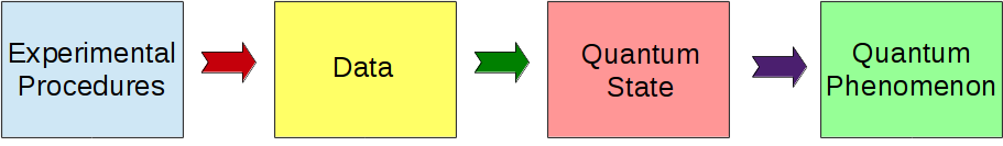
Figure 1: The analysis of many experiments in quantum physics can be divided into several steps, from the experimental procedures to the verification of quantum mechanical properties of the generated states.

2 Systematic errors in quantum experiments

In this first part of the article, we discuss what assumptions are typically used in quantum experiments. The violation of these assumptions leads to systematic errors and we show how these systematic errors can be identified using statistical methods and hypothesis tests.

2.1 Assumptions underlying quantum experiments

Before explaining the assumptions, it is useful to discuss a simple example. Consider a two-photon experiment, where a quantum state should be analysed by performing state tomography. For that, Alice and Bob have to measure all the nine possible combinations of the Pauli matrices $\sigma_{i}\otimes\sigma_{j}$ for $i,j\in\{x,y,z\}$. In practice, this can be done as follows: Alice and Bob measure the three Pauli matrices $\sigma_{x},\sigma_{y},\sigma_{z}$ by measuring the polarization in different directions, getting the possible results $+$ and $-$. These results correspond to the projectors on the eigenvectors of the observable. By combining the results, they obtain one of four possible outcomes from the set $\{++,+-,-+,--\}$. The measurement is repeated $N$ times on copies of the state, where the outcome $++$ occurs $N_{++|ij}$ times etc. From that, one can obtain the relative frequencies $F_{++|ij}=N_{++|ij}/N$ and estimate the expectation values as $\langle{\sigma_{i}\otimes\sigma_{j}}\rangle_{\rm exp}=(N_{++|ij}-N_{+-|ij}-N_{-+|ij}+N_{--|ij})/N.$ In addition, the expectation values of the marginals $\sigma_{i}\otimes\sigma_{0}$ (here and in the following, we set $\sigma_{0}=\mathbb{1}$) can be determined from the same data. Given all the experimental results, Alice and Bob may then reconstruct the quantum state via the formula

$$\hat{}\varrho=\frac{1}{4}\sum_{i,j\in\{0,x,y,z\}}\!\!\!\lambda_{ij}\sigma_{i}\otimes\sigma_{j},\mbox{ where }\lambda_{ij}=\langle{\sigma_{i}\otimes\sigma_{j}}\rangle_{\rm exp}.$$ (1)

This simple quantum state reconstruction scheme is often called linear inversion. It assumes that the observed frequencies equal the probabilities, we will discuss its advantages and disadvantages below. For the moment, we just use it as an example to illustrate the definitions and discussion concerning systematic errors in experiments.

Now we can formulate the assumptions that lead to the statistical model typically used in quantum experiments. We consider a scenario where one actively chooses between different measurements (e.g., the $\sigma_{i}\otimes\sigma_{j}$), each having a finite number of results. We use the label $s$ to denote the measurement setting and $r$ to denote the result. It is important to note that, if in an experiment using the setting $s$ one registers the result $r$, then this outcome $r|s$ is not just treated as a classical result. In addition, each outcome is tied to an operator $M_{r|s}$ (e.g., the projectors onto the eigenstates corresponding to the results $\{++,+-,-+,--\}$ of $\sigma_{i}\otimes\sigma_{j}$) that serves as the object to compute probabilities within quantum mechanics: If the underlying quantum state is characterized by the density operator $\varrho$, then the probability to observe $r|s$ is given by $P(r|s;\varrho)=\tr(\varrho M_{r|s})$. Therefore, this quantum mechanical description is one of the essential ingredients to connect the observed samples with the parameters of the system that one likes to infer. Knowledge about this description can come from previous calibration measurements or from other expertise that one has acquired with the equipment. But one thing should be obvious: If one assumes a description $M_{r|s}$, which deviates from the true description in the experiment $\tilde{M}_{r|s}$, then things can go terribly wrong and these type of errors are the ones that we like to address in the following.

Clearly, such deviations are presumably present in any model, but they are usually assumed to be small. However, considering the increased complexity of present experiments, one can ask the question, whether or not these deviations show up significantly in the data. Well known examples, like different detection efficiencies or dark-count rates in photo-detectors or non-perfect gate fidelities for single-qubit rotations preceding the readout of a trapped ion, could support this scepticism. However, these effects are hardly ever considered in the description of $M_{r|s}$.

Let us complete the list of assumptions. Most often each experiment of setting $s$ is repeated $N$ times, which are assumed to be independent and identically distributed trials. So one further assumes that one always prepares the same quantum state $\varrho$, measures the same observables $M_{r|s}$, and that both are completely independent . Clearly, also in all these steps there can be errors, for instance, due to drifts in the measuring devices or dead-times in detectors coming from previous triggering events. However, if everything works as planned, then it is not necessary anymore to keep track of the individual measurement results, since every information that can be inferred about the state parameters is already included in the count rates $N_{r|s}$ of the individual measurement results $r|s$. Their probability is then given by a multinomial distribution ${\rm Mult}[N,P(r|s;\varrho)]$ for each setting, which is the distribution characterizing $N$ repetitions of independent trials. Here, the single event probabilities $P(r|s;\varrho)=\tr(\varrho M_{r|s})$ are calculated according to quantum mechanics and these are the only parameters that depend on the quantum state.

Finally, the whole collection of distributions for all measurement settings is the exact parametric model used for most quantum experiments. These distributions are given by the set

$$\mathcal{P}_{\rm QM}=\Big{\{}P(\{N_{r|s}\}_{r,s};\varrho)=\prod_{s}{\rm Mult}\left[N,\tr(\varrho M_{r|s})\right],\mbox{ for all }\varrho\mbox{ with }\varrho~{}\geq~{}0,\tr(\varrho)=1\Big{\}},$$ (2)

and the observed probabilities are assumed to be an element of this set. In the following, we discuss how the validity of this model can be tested.

2.2 Testing the assumptions

How can one test in this framework whether the assumed measurement description is correct for the experiment? As a first try, we could intersperse the experiment with test measurements, in which one prepares previously characterized states. But such an option seems very cumbersome, independent of problems like how to characterize the test states in the first place and to ensure that they are well prepared in between the true experiment. In contrast, we want to do it more directly and this becomes possible, at least partially, by exploiting that quantum states only allow a restricted set of event probabilities.

Let us first discuss the idea for the case where one has access to the true event probabilities $P_{0}(r|s)$ which can be attained from the relative frequencies $F_{r|s}=N_{r|s}/N\to P_{0}(r|s)$ in the limit $N\to\infty$. We want to know whether these observed probabilities are at all compatible with the assumed measurement description. This boils down to the question whether there exists a quantum state $\varrho_{0}$ with $P_{0}(r|s)=\tr(\varrho_{0}M_{r|s})$ for all $r,s$. Since quantum states must respect the positivity constraint $\varrho\geq 0$, not all possible probabilities are accessible: For instance, if one measures a qubit along the $x,y,z$ directions, its corresponding probabilities will be constrained by the requirement that the Bloch vector must lie within the Bloch ball. To make this more general, assume that we have a certain set of numbers $w_{r|s}$ such that the observable $\sum_{r|s}w_{r|s}M_{r|s}\geq 0$ has no negative eigenvalues and is, therefore, positive semidefinite. If the probabilities $P_{0}(r|s)$ can indeed by realized by a quantum state, one has

$$w\cdot P_{0}\equiv\sum_{r,s}w_{r|s}P_{0}(r|s)=\sum_{r,s}w_{r|s}\tr(\varrho_{0}M_{r|s})=\tr[\varrho_{0}\big{(}\sum_{r,s}w_{r|s}M_{r|s}\big{)}]\geq 0,$$ (3)

where the inequality holds because both operators are positive semidefinite. Thus, if everything is correct one must get a non-negative value for $w\cdot P_{0}\geq 0$. Consequently, whenever one observes $w\cdot P_{0}<0$, one knows that something must be wrong and that the description of the measurements $M_{r|s}$ has some flaws. This type of inequalities is similar in spirit to Bell inequalities for local hidden variable models or entanglement witnesses for separable states [2, 3]. Let us point out that the above inequalities are necessary and sufficient. So, indeed any $P_{0}(r|s)$ which cannot originate from a quantum state, can be detected by appropriately chosen coefficients $w_{r|s}$ by $w\cdot P_{0}<0$ [4]. Finally, we add that besides the positivity, some other constraints for the measurement description are conceivable. For instance, in the example of state tomography from above, the marginal $\langle{\sigma_{x}\otimes\sigma_{0}}\rangle$ should not depend on whether it has been derived from the measurement $\sigma_{x}\otimes\sigma_{x}$ or $\sigma_{x}\otimes\sigma_{y}$. This can be formulated as a linear dependency of the form $\sum_{r,s}w_{r|s}M_{r|s}=0$ and the corresponding constraint even becomes an equality $w\cdot P_{0}=0$.

Note that, with this test we ask the question whether the data $P_{0}(r|s)$ fit at all to the assumed measurement model $M_{r|s}$. But it should be clear that this approach can never serve as a proof that everything is correct in the experiment. For example, one can consider again the Bloch ball, where the measurement model assumes perfectly aligned measurements in the $x,y,z$ directions, but in the true experiment one measures in slightly tilted directions which distorts the resulting Bloch ball. All states from this tilted Bloch ball, which lie outside the standard sphere, will be detected by the above method as being incompatible with the assumed model. For all other states, however, we do not see the difference because they are still consistent with the model.

Finally, let us address the point that we only collect count rates in the experiment. Since the relative frequencies $F_{r|s}$ are only approximations to the true probabilities $P(r|s)$, it is clear that a similar inequality as Eq. (3) does not need to hold anymore for $w\cdot F$, even if everything is correct. One would expect, however, that larger negative values are much less likely. This is indeed the case and is made more quantitative via Hoeffding’s inequality [5].

This inequality states the following: Consider $N$ independent, not necessarily identically distributed, bounded random variables $X_{i}\in[a_{i},b_{i}].$ Then the sample mean $\bar{X}=\sum_{i}X_{i}/N$ satisfies

$${\rm Prob}[\bar{X}-\mathbbm{E}(\bar{X})\leq-t]\leq\exp\Big{(}\frac{-2t^{2}N^{2}}{\sum_{i}(b_{i}-a_{i})^{2}}\Big{)}$$ (4)

for all $t>0$, where $\mathbbm{E}(\bar{X})$ denotes the expectation value of $\bar{X}$. In practice, the main statement of this inequality is that for $N$ independent repetitions of an experiment, the probability of deviations from the mean value by a difference $t$ scales like $\exp(-t^{2}N).$ It is important to stress that this result uses no extra assumptions, like $N$ being large, at all.

For our case, we can use Hoeffding’s inequality to bound the probability of observing data that violate positivity constraints as in Eq. (3). More precisely, we can derive the following statement [6]: For all distributions compatible with quantum mechanics, the probability to observe frequencies $\{F_{r|s}\}_{r,s}$ such that $w\cdot F<-\varepsilon$ is bounded by

$${\rm Prob}_{P}\big{[}w\cdot F<-\varepsilon\big{]}\equiv\sum_{\stackrel{{\scriptstyle\{n_{r|s}\}_{r,s}:}}{{w\cdot F<-\varepsilon}}}P(\{n_{r|s}\}_{r,s})\leq\exp\Big{(}-\frac{2\varepsilon^{2}N}{C_{w}^{2}}\Big{)},\mbox{ for all }P\in\mathcal{P}_{QM}$$ (5)

with $C_{w}^{2}=\sum_{s}(w_{{\rm max}|s}-w_{{\rm min}|s})^{2}$ and $w_{{\rm max}|s}$, $w_{{\rm min}|s}$ being the extreme values of $\{w_{r|s}\}_{r}$. Again, this can be interpreted as showing that if everything is correct, then the probability of finding a violation of the positivity constraint is exponentially suppressed.

We can use this statement as follows: Suppose that we should reach a conclusion whether the observed data are “compatible” or “incompatible” with our assumed model. Of course, if we say “incompatible”, we do not want to reach this conclusion too often, if indeed everything is perfect. For definiteness, we may assume that the probability of claiming incompatibility if everything is correct should be at maximum $\alpha=1\%$. We then use Eq. (5) to deduce the threshold value that we need to beat, $\varepsilon_{\alpha}=\sqrt{C_{w}^{2}|\log(\alpha)|/2N}$. If we now carry out the experiment and register click rates with $w\cdot F<-\varepsilon_{\alpha}$, we know that there was at most a $\alpha=1\%$ chance that we would have registered such badly looking data, if everything is correct. Since this would be really bad luck we would rather say “incompatible”, and assume that some systematic error was present .

In practice, this test can be used to detect systematic errors in various scenarios: In ion trap experiments, a typical systematic error comes from the cross talk between the ions, i.e. the fact that a laser focused on one ion also influences the neighbouring ions. This phenomenon can be detected with the presented method [6]. The second application are Bell experiments: In these experiments, the choice of the measurements on one party should ideally not influence the results of the other party and a violation of this condition completely invalidates the result of a Bell test. Again, this non-signalling condition can be formulated as linear constraints on the probabilities and this can be tested with the presented method. In all these applications, the determination of the vector $w$ characterizing the positivity constraint or the linear constraint can be done as follows: One splits the observed data into two parts. From the first part one determines the $w$ leading to the maximal violation of the respective constraint for the first half. Then, one applies this $w$ as a test to the second part of the data. If the violations of the constraint are only due to statistical fluctuations, the respective $w$ for the two parts of the data are uncorrelated and the test will not find a significant violation of the constraint.

Let us point out that the mathematical framework just described is called a hypothesis test [7], in which one tests the null-hypothesis $N_{0}$: “compatible”, against the alternative $A$: “incompatible”. The special property of such a test is that there is an asymmetry about the two types of errors that can occur. As already explained, our concern is that, when saying “incompatible”, then this statement is more or less correct. The other error can occur when we respond “compatible” to incompatible data. Naturally, this error characterizing the detection strength of our test, ideally, should also be made small. However, it is not possible to reduce both errors equally simultaneously. Nevertheless, since we cannot detect all possible systematic deviations from the assumed model, anyway, one should not be too euphoric about the statement “compatible” in this sense.

Note that, while the presented test has been build up by first deriving specific inequalities for event probabilities and then equipping it with the necessary statistical rigour to arrive at an hypothesis test, one can also take the other direction, by using techniques which are known to be good for hypothesis tests and apply them to the special statistical model of the quantum experiments. We have done this for the so-called generalized likelihood-ratio test [7] and details can be found in Ref. [6]. Finally, other tests for systematic errors can be found in Refs. [8, 9, 10].

3 Performing state tomography

In the previous section, we have seen that care has to be taken when making the measurements on the quantum system. In this section, we show that the interpretation of tomographic data, such as the reconstruction of the quantum state, has to be done with care, too. Otherwise, one introduces yet another class of systematic errors.

3.1 Problems with state estimates

We are used to summarize experimental data by an estimate together with an error margin. In quantum state tomography this corresponds to an estimate for the density matrix together with an error region. So, the first question is how one can obtain an estimate $\hat{}\varrho$ for the experimentally prepared density matrix $\varrho_{\exp}$ from the observed frequencies $F_{r|s}.$ The simplest approach is to use linear inversion, that is, the method given in Eq. (1). This has, however, at first sight some disadvantages: Due to statistical fluctuations the observed frequencies are not equal to the true probabilities and this leads to the consequence that the reconstructed “density matrix” will typically have some negative eigenvalues. This makes the further analysis of the experiment, e.g. the evaluation of entanglement measures, not straightforward. In order to circumvent this, one often makes a density matrix reconstruction by setting

$$\hat{}\varrho=\arg\max_{\sigma\geq 0}\mathcal{F}(F_{r|s},\sigma).$$ (6)

Here, one optimizes a target function $\mathcal{F}$ over all density matrices $\sigma$ and the optimal $\sigma$ will obviously be a valid density matrix. Examples for this type of state reconstruction are the maximum-likelihood reconstruction or the least-squares reconstruction, both are frequently used for experiments in quantum optics.

An important property of such an estimator is the question whether it is biased or unbiased. This means the following: The underlying state $\varrho_{\rm exp}$ leads via the multinomial distribution to a probability distribution over the frequencies $F_{r|s}$. The estimator $\hat{}\varrho$ is a function from the observed data (the frequencies $F_{r|s}$) to the state space. In this way, the original state $\varrho_{\rm exp}$ induces a probability distribution over the estimators $\hat{}\varrho$, and one can ask whether the expectation value of this equals the original state, $\mathbbm{E}[\hat{\varrho}]\stackrel{{\scriptstyle?}}{{=}}\varrho_{\text{exp}}.$ If this is the case, the estimator is unbiased, otherwise it is biased. It must be stressed, however, that biased estimators are not necessarily useless or bad, as it all depends on the purpose the estimator is used for.

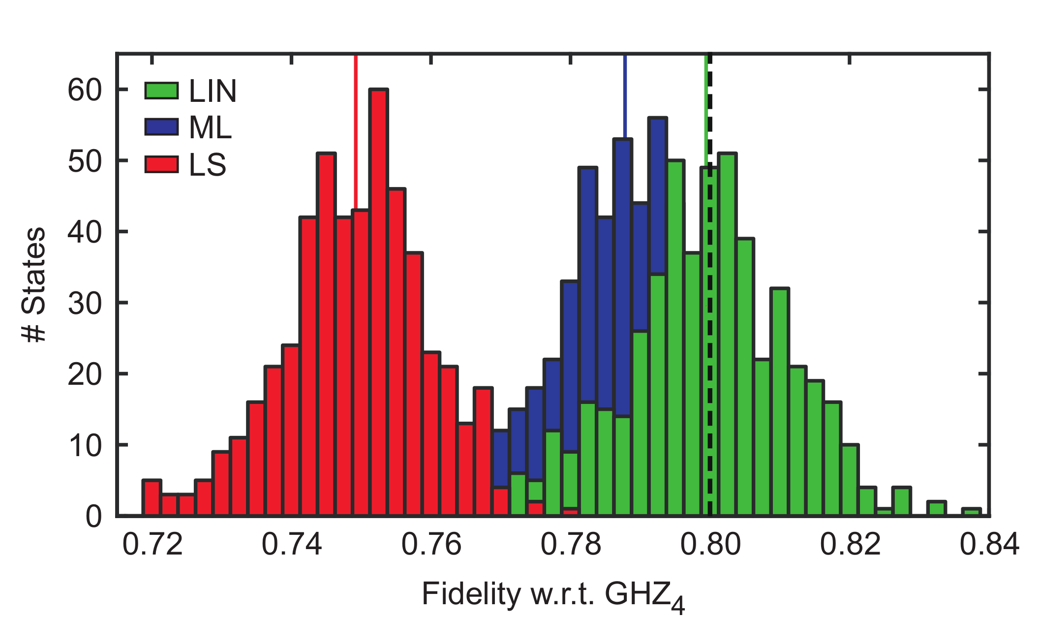
Figure 2: Demonstration of the bias for different state estimators. A given state $\varrho_{\rm exp}$ having 80% fidelity with the GHZ state was used to sample the distribution of the estimator $\hat{}\varrho$ in state space, and from these samples the fidelities with the GHZ state were computed. The maximum-likelihood (ML) and least-square (LS) estimators clearly underestimate the fidelity, while the linear inversion (LIN) is unbiased. The figure is taken from Ref. [11].

For quantum state reconstruction one can prove the following: Any state reconstruction scheme that yields a density matrix from experimental data will be biased, i.e., on average, the reconstructed state $\hat{\varrho}$ will not be the state used in the experiment, $\mathbbm{E}[\hat{\varrho}]\neq\varrho_{\text{exp}}$. A proof of this statement was given in Ref. [11], but the following example demonstrates that the problem in finding an unbiased estimator comes from the fact that the quantum mechanical state space is bounded by the positivity constraint. Consider a coin toss where we are interested in the modulus of the difference between the probability of obtaining heads or tails, $\Delta=|p_{h}-p_{t}|=1-2\min\{p_{h},1-p_{h}\}$. This quantity cannot be negative, so also an estimator should not be negative. Let us assume that an estimator $\hat{\Delta}$ is unbiased, $\mathbbm{E}[\hat{\Delta}]=\Delta_{\text{exp}}$. Then, for any experimental data that could come from a fair coin ($\Delta_{\text{exp}}=0$) we cannot have $\hat{\Delta}>0$ since this would imply $\mathbbm{E}[\hat{\Delta}]=\sum_{k}(1/2)^{n}(\begin{smallmatrix}n\\ k\end{smallmatrix})\hat{\Delta}(k)>0$, where $k$ denotes the number of occurrences of heads. On the other hand, any possible number of heads and tails is compatible with a fair coin. So, the estimate $\hat{\Delta}$ for any data must be 0. Then in particular $\mathbbm{E}[\hat{\Delta}]=0$, which means that $\hat{\Delta}$ is a biased estimator whenever the coin is not fair.

Apart from this theoretical argument, the question arises whether this effect plays a significant role in practical quantum state reconstruction. Unfortunately, this is the case and this effect can causes substantial fidelity underestimation or spurious entanglement detection in realistic scenarios [11]. This problem applies to the established schemes for reconstructing a density matrix, in particular to the maximum-likelihood method [12] and the constrained least-squares method [13]. So, how large is the bias? For example, in a tomography of a four-qubit GHZ state with fidelity $0.8$, when reconstructing from a total number of 8100 samples, the state from a maximum-likelihood estimate has a fidelity of $0.788\pm 0.010$ [11], i.e., the fidelity is systematically underestimated (see also also Fig. 2). Such an underestimation may be considered to be unfortunate, but acceptable. However, it was also demonstrated that maximum-likelihood and least-square methods tend to overestimate the entanglement. In fact, for a clearly separable state the reconstructed states can be always entangled, thus leading to spurious entanglement detection [11]. This is not acceptable for many experiments.

A way to avoid the bias is to accept that the reconstructed density matrix is not always a valid quantum state and can have negative eigenvalues. The simplest unbiased method is linear inversion explained above. More generally, if $M_{r|s}$ are the operators corresponding to the measurement outcomes in a complete tomographic measurement scheme, then one can find operators $X_{r|s}$ such that for all states $\varrho=\sum_{r|s}X_{r|s}P(r|s;\varrho)$ holds, generalizing Eq. (1) . The estimate given by linear reconstruction is then $\hat{\varrho}=\sum_{r|s}X_{r|s}F_{r|s}$, where $F_{r|s}$ are the relative frequencies of the result $r$ for setting $s$. This estimate is unbiased but it comes with the price that in all realistic scenarios $\hat{\varrho}$ has some negative eigenvalues and hence it is not a valid density matrix. Depending on the intended use of the reconstructed density matrix this may be problematic, but it was shown in Ref. [11] that entanglement measures or the Fisher information can still be estimated. In addition, we stress that the eigenvectors corresponding to these negative eigenvalues are randomly distributed in the following sense: If we choose a rank one projection $|\alpha\rangle\!\langle\alpha|$ independently of the data, then the probability that $\tr(\hat{\varrho}|\alpha\rangle\!\langle\alpha|)<-\epsilon$ is exponentially suppressed, as can be seen from the inequality in (3).

3.2 Problems with error regions

Any report of an experiment has to equip the reported results with error bars. In the case of a density matrix, this will be a high-dimensional error region. When specifying an error region, one first has to decide between the Bayesian framework and the frequentistic framework. A Bayesian analysis gives a credible region, which has the property that with high probability the actual state is in this region. A frequentist’s analysis gives a confidence region, which is a map from the data to a region in state space such that with high probability the region contains the actual state. There is a long debate in mathematical statistics which method is appropriate, but most of the subsequent discussion is independent of this dispute.

Before discussing the advantages and disadvantages of an error region, it is important to remember, that the variance does in general not give an appropriate error region. This occurs in particular if the underlying distributions are far from being Gaussian. But for state tomography, the data is sampled from a multinomial distribution, typically with a very low number of events. Indeed, in many experiments the number of clicks per measurement outcome is about ten, but sometimes even below one. Also the method of bootstrapping may yield an inappropriate error region. In bootstrapping, one uses an estimate $\hat{\varrho}$ for the state (parametric bootstrapping) or the empirical distributions of the outcomes of the measurements $F_{r|s}$ (non-parametric bootstrapping) in order to estimate the variance of the estimate. This estimate is usually obtained by Monte Carlo sampling from the corresponding distributions. There is no particular reason that this should be a good error region, and it was also demonstrated that the most commonly used schemes yield invalid error regions.

Methods to obtain valid error regions both in the Bayesian [14] and in the frequentistic framework [15] have been suggested, however, they turn out to be notoriously difficult to compute. But even when it is possible to achieve a proper error region, one has to keep in mind that the size of the error region scales with the dimension of the underlying Hilbert space, i.e., exponentially with the number of qubits. This makes it very difficult to perform state tomography of a large system with a reasonable sized error region. Fortunately, in many situations the error region for the state is not of uttermost importance. Often one is only interested in certain scalar quantities like a measure of entanglement or the fidelity with the (pure) target state. In this cases it is possible to infer an appropriate confidence region directly from the data, without taking the detour over an error region for the density operator. This is particularly simple, if the quantity of interest is linear in the density matrix, e.g., the fidelity with a pure state $F=\langle\psi|\varrho|\psi\rangle$. One can again use Hoeffding’s tail inequality in order to obtain a lower bound $\hat{F}_{l}$ on the fidelity. The promise is then that $P(\hat{F}_{l}>\langle\psi|\varrho_{\mathrm{exp}}|\psi\rangle)<1\%$ for any state $\varrho_{\mathrm{exp}}$. A general method to provide such confidence regions for convex functions, like the bipartite negativity or the quantum Fisher information, has been introduced in Ref. [11].

4 Analysing density matrices

In the last section of this article, we assume that a valid multiparticle density matrix $\varrho$ is given and the task is to analyse its properties. Naturally, many questions can be asked about a density matrix, but we concentrate on two of them. First, we consider the question whether the state is genuinely multiparticle entangled or not. We explain a powerful approach for characterizing multiparticle entanglement with the help of so-called PPT mixtures and semidefinite programming. Second, we consider the problem of characterizing the complexity of a given quantum state and explain an approach using exponential families. For example, in this approach a state that is a thermal state of a Hamiltonian with two-body interactions only, is considered to be of low complexity and the distance to these thermal states can be considered as a measure of complexity. The underlying techniques also allow to characterize pure states which are not ground states of a two-body Hamiltonian.

4.1 Characterizing entanglement with PPT mixtures

4.1.1 Notions of entanglement —

Before explaining the characterization of multiparticle entanglement, we have to explain some basic facts about entanglement on a two-particle system. The definition of entanglement is based on the notion of local operations and classical communication (LOCC). If a quantum state can be prepared by LOCC, it is called separable, otherwise it is entangled. For pure states, this just means that product states of the form $|\phi\rangle=|\alpha\rangle\otimes|\beta\rangle$ are separable and all other states (e.g. the singlet state $|\psi^{-}\rangle=(|01\rangle-|10\rangle)/\sqrt{2}$) are entangled. If mixed states are considered, a density matrix $\varrho$ is separable, if it can be written as a convex combination of product states,

$$\varrho=\sum_{k}p_{k}\varrho_{A}^{k}\otimes\varrho^{k}_{B},$$ (7)

where the $p_{k}$ form a probability distribution, so they are non-negative and sum up to one. Physically, the convex combination means that Alice and Bob can prepare the global state by fixing the joint probabilities with classical communication and then preparing the states $\varrho^{A}_{k}$ and $\varrho^{B}_{k}$ separately. The question whether or not a given quantum state is entangled is, however, in general difficult to answer. This is the so-called separability problem [2, 3].

Many separability criteria have been proposed, but none of them delivers a complete solution of the problem. The most famous separability test is the criterion of the positivity of the partial transpose (PPT criterion) [16]. For that, one considers the partial transposition of a density matrix $\varrho=\sum_{ij,kl}\varrho_{ij,kl}|i\rangle\langle j|\otimes|k\rangle\langle l|$, given by

$$\varrho^{T_{A}}=\sum_{ij,kl}\varrho_{ij,kl}|j\rangle\langle i|\otimes|k\rangle\langle l|.$$ (8)

In an analogous manner, one can also define the partial transposition $\varrho^{T_{B}}$ with respect to the second system. The PPT criterion states that for any separable state $\varrho$ the partial transpose $\varrho^{T_{A}}$, (and consequently also $\varrho^{T_{B}}=(\varrho^{T_{A}})^{T}$) has no negative eigenvalues and is therefore positive semidefinite. So, if one finds a negative eigenvalue of $\varrho^{T_{A}}$, then the state $\varrho$ must necessarily be entangled. The PPT criterion solves the separability problem for low dimensional systems (that is, two qubits or one qubit and one qutrit) [2], but in all other cases the set of separable states is a strict subset of the PPT states. The entangled states which are PPT are of great theoretical interest: It has been shown that their entanglement can never be distilled to pure state entanglement, even if many copies of the state are available. This weak form of entanglement is then also called bound entanglement and bound entangled states are central for many challenging questions in quantum information theory.

The characterization of entanglement becomes significantly more complicated, if more than two particles are involved. Let us consider three particles (A, B, C). First, a state can be fully separable, meaning that it does not contain any entanglement and is of the form $|\phi^{\rm fs}\rangle=|\alpha\rangle\otimes|\beta\rangle\otimes|\gamma\rangle$. If a state is entangled, one can further ask whether only two parties are entangled or all three parties. For instance, in the state $|\phi^{\rm bs}\rangle=|\psi^{-}\rangle_{AB}\otimes|\gamma\rangle_{C}$ the parties A and B are entangled, but C is not entangled with A or B, therefore the state is called biseparable. Alternatively, if all parties are entangled with each other, the state is called genuine multipartite entangled [3]. For the simplest case of three two-level systems (qubits) it has been shown that even the genuine multipartite entangled states can be divided into two subclasses, represented by the GHZ state $|GHZ\rangle=(|000\rangle+|111\rangle)/\sqrt{2}$ and the W state $|W\rangle=(|001\rangle+|010\rangle+|100\rangle)/\sqrt{3}$. These subclasses are distinguished by the fact that a single copy of a state in one class cannot be converted via LOCC into a state in the other class, even if this transformation is not required to be performed with probability one [3].

The classification of entanglement for pure states can be extended to mixed states by considering convex combinations as in Eq. (7). First, a mixed state is fully separable, if it can be written as a convex combination of fully separable states

$$\varrho^{\rm fs}=\sum_{k}p_{k}\varrho^{k}_{A}\otimes\varrho^{k}_{B}\otimes\varrho^{k}_{C},$$ (9)

and a state is biseparable, if it can be written as a mixture of biseparable states, which might be separable with respect to different partitions,

$$\varrho^{\rm bisep}=p_{1}\varrho^{\rm sep}_{A|BC}+p_{2}\varrho^{\rm sep}_{B|AC}+p_{3}\varrho^{\rm sep}_{C|AB}.$$ (10)

The different notions of entanglement in the multipartite case and the different bipartitions that have to be taken into account imply that the question whether a given mixed multipartite state is entangled or not is extraordinarily complicated.

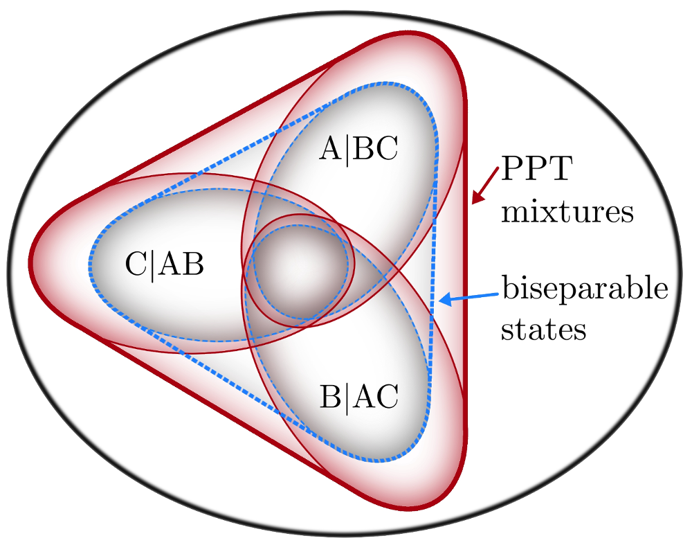
Figure 3: Schematic view of the states which are PPT mixtures and the biseparable states for three particles. There are three possible bipartitions, and the corresponding sets of states which are separable or PPT for the bipartition. The figure is taken from Ref. [17].

4.1.2 The approach of PPT mixtures —

A systematic approach for characterizing genuine multiparticle entanglement makes use of so-called PPT mixtures [17]. Instead of asking whether a state is a mixture of separable states with respect to different partitions as in Eq. (10), one asks whether it is a mixture of states which are PPT for the bipartitions

$$\varrho^{\rm pptmix}=p_{1}\varrho^{\rm ppt}_{A|BC}+p_{2}\varrho^{\rm ppt}_{B|AC}+p_{3}\varrho^{\rm ppt}_{C|AB}.$$ (11)

Since the separable states are a subset of the PPT states, any biseparable state is also a PPT mixture. This means that if a state is no PPT mixture, then it must be genuine multipartite entangled (see also Fig. 3).

At first, it is not clear what can be gained by this redefinition of the problem. First, the condition for PPT mixtures is a relaxation of the definition of biseparability and it might be that the conditions are relaxed too much, implying that not many states can be detected by this method. Second, it is not clear how the criterion for PPT mixtures can be evaluated in practice and whether this is easier than evaluating the conditions for separability directly. In the following, however, we will see that the question whether a state is a PPT mixture or not can directly be checked with a technique called semidefinite programming. Furthermore, the approximation to the biseparable states is rather tight, and for many families of states the property of being a PPT mixture coincides with the property of being biseparable.

4.1.3 Evaluation of the criterion —

Let us discuss the evaluation of the condition for PPT mixtures. For that, we need to introduce the notion of entanglement witnesses. In the two-particle case, an entanglement witness $\mathcal{W}$ is an observable with the property that the expectation value is positive for all separable states, $\tr(\varrho^{\rm sep}\mathcal{W})\geq 0$. This implies that a measured negative expectation value signals the presence of entanglement. In this way, the concept of an entanglement witness bears some similarity to a Bell inequality, where correlations are bounded for classical states admitting a local hidden variable model, while entangled states may violate the bound.

How can entanglement witnesses be constructed? For the two-particle case a simple method goes as follows: Consider an observable of the form

$$\mathcal{W}=P+Q^{T_{A}},$$ (12)

where $P\geq 0$ and $Q\geq 0$ are positive semidefinite operators. Using the fact that $Tr(XY^{T_{A}})=Tr(X^{T_{A}}Y)$ for arbitrary operators $X,Y$, we find that for a separable state $Tr(\mathcal{W}\varrho^{\rm sep})=Tr(P\varrho^{\rm sep})+Tr(Q(\varrho^{\rm sep})^{T_{A}})\geq 0,$ since $\varrho^{\rm sep}$ has to be PPT. Therefore, the observable $\mathcal{W}$ is an entanglement witness, which may be used to detect the entanglement in states that violate the PPT criterion.

This construction can be used to decide whether a given three-particle state is a PPT mixture or not. For that, consider the optimization problem

$$\underset{\mathcal{W},P_{i},Q_{i}}{\mbox{minimize}} Tr(\varrho\mathcal{W})$$

subject to: $$\mathcal{W}=P_{1}+Q_{1}^{T_{A}}=P_{2}+Q_{2}^{T_{B}}=P_{3}+Q_{3}^{T_{C}}\mbox{ and }$$ (13)

$$P_{i}\geq 0\mbox{ for }i=1,2,3\mbox{ and }$$

$$\mathbb{1}\geq Q_{i}\geq 0\mbox{ for }i=1,2,3.$$

The constraints guarantee that the observable $\mathcal{W}$ is of the form as in Eq. (12) for any of the three bipartitions. This means, that if a state is a PPT mixture as in Eq. (11), the expectation value $Tr(\varrho\mathcal{W})$ has to be non-negative. On the other hand, one can show that if a state is not a PPT mixture, then the minimization problem will always result in a strictly negative value [17]. In this way, the question whether a state is a PPT mixture or not, can be transformed into a optimization problem under certain constraints.

The point is that the optimization problem belongs to the class of semidefinite programs (SDP). An SDP is an optimization problem of the type

$$\underset{x_{i}}{\mbox{minimize}} \sum_{i}c_{i}x_{i}$$

subject to: $$F_{0}+\sum_{i}x_{i}F_{i}\geq 0,$$ (14)

where the $c_{i}$ are real coefficients defining the target function, the $F_{i}$ are hermitean matrices defining the constraints and the $x_{i}$ are real coefficients which are varied. This type of optimization problem has two important features [18]. First, using the so-called dual problem one can derive a lower bound on the solution of the minimization, which equals the exact value under weak conditions. This means that the optimality of a solution found numerically can be demonstrated. In this way, one can prove rigorously by computer whether a given state is a PPT mixture or not. Second, for implementing an SDP in practice there are ready-to-use computer algebra packages available and therefore the practical solution of the SDP is straightforward.

4.1.4 Results —

Concerning the characterization of PPT mixtures, the following results have been obtained:

• First, the practical evaluation of the SDP in Eq. (13) can be carried out easily with standard numerical routines. A free ready-to-use package called PPTMixer is available online [19], and it solves the problem for up to six qubits on standard computers. For a larger number of particles, the numerical evaluation becomes difficult, but analytical approaches are also feasible [17, 22].

• For many families of states, the approach of the PPT mixtures delivers the strongest criterion of entanglement known so far. For many cases it even solves the problem of characterizing multiparticle entanglement. For instance, three-qubit permutation-invariant states are biseparable, if and only if they are PPT mixtures [20]. The same holds for states with certain symmetries, like GHZ diagonal states or four-qubit states diagonal in the graph-state basis [22, 21].

• Nevertheless, the approach of PPT mixtures can not detect all multiparticle entangled states. There are examples of genuinely entangled three-qubit and three-qutrit states, which are PPT mixtures [23, 24]. For an increasing dimension and number of particles one can even show that the probability that a given multiparticle entangled state can be detected by the PPT mixture approach decreases [25]. This finding, however, is in line with the observation that also in bipartite high-dimensional systems no single entanglement criterion detects a large fraction of states [26].

• The value $\mathcal{N}(\varrho)=-Tr(\varrho\mathcal{W})$, that is, the amount of violation of the witness condition is a computable entanglement monotone for genuine multiparticle entanglement [22]. It can be called the genuine multiparticle negativity, as it generalizes the entanglement measure of bipartite negativity.

• An interesting feature of the PPT mixer approach is that it can also be evaluated, if only partial information on the state $\varrho$ is available. Namely, if only the expectation values $\langle{A_{i}}\rangle$ of some observables $A_{i}$ are known, one can add in the SDP in Eq. (13) that the witness $\mathcal{W}$ should be a linear combination of the measured observables $\mathcal{W}=\sum_{i}\lambda_{i}A_{i}$. It can be shown that this is then still a complete solution of the problem, meaning that the SDP returns a negative value, if and only if all states that are compatible with the data $\langle{A_{i}}\rangle$ are not PPT mixtures.

4.2 Characterizing the complexity of quantum states

Besides the question whether a given multiparticle quantum state is entangled or not, one may also be interested in other questions about a reconstructed quantum state $\varrho$. For instance, one may ask: Is the given state is a ground state or thermal state of a simple Hamiltonian? In the following, we will explain how this question can be used to characterize the complexity of a many-body quantum state.

4.2.1 Exponential families —

First, one can consider the set of all possible two-body Hamiltonians. For multi-qubit systems they are of the form

$$H_{2}=\sum_{i,\alpha}\lambda^{(i)}_{\alpha}\sigma^{(i)}_{\alpha}+\sum_{i,j,\alpha,\beta}\mu^{(ij)}_{\alpha\beta}\sigma^{(i)}_{\alpha}\sigma^{(j)}_{\beta}+\nu\mathbb{1},$$ (15)

where $\sigma_{\alpha}^{(i)}$ is the Pauli matrix $\sigma_{\alpha}$ acting on the $i$-th qubit. This Hamiltonian $H_{2}$ contains, apart from the identity, single-particle terms and two-particle interactions. However, no geometrical arrangement of the particles is assumed and the two-particle interactions are between arbitrary particles and not restricted to nearest-neighbour interactions. We also denote the set of all two-particle Hamiltonians by $\mathcal{H}_{2}$, and in a similar manner one can define the sets of $k$-particle Hamiltonians $\mathcal{H}_{k}$.

Given the set of $k$-particle Hamiltonians, we can define the so-called exponential family of all thermal states

$$\mathcal{Q}_{k}=\{\exp\{H_{k}\}\mbox{ with }H_{k}\in\mathcal{H}_{k}\},$$ (16)

where the normalization of the state has been included into the Hamiltonian via the term $\nu\mathbb{1}$.

If a given quantum state is in the family $\mathcal{Q}_{k}$ for small $k$, then one can consider it to be less complex, since only a simple Hamiltonian with few parameters are required to describe the interaction structure. One the other hand, if a state is not in the exponential family, one can consider the distance

$$D_{k}(\varrho||\mathcal{Q}_{k}):=\inf_{\eta\in\mathcal{Q}_{k}}D(\varrho||\eta)$$ (17)

with $D(\varrho||\eta)=\tr[\varrho\log(\varrho)]-\tr[\varrho\log(\eta)]$ being the relative entropy, as a measure of the complexity of the quantum state. The optimal $\eta$ is also called the information projection $\tilde{}\varrho_{k}$ and one can show that this $\tilde{}\varrho_{k}$ is the maximum likelihood approximation of $\varrho$ within the family $\mathcal{Q}_{k}$ [27]. Below, we will explain several further equivalent characterizations which can help to solve the underlying minimization problem.

This type of complexity measure has been first discussed for the case of classical probability distributions in the context of information geometry [28]. The measure $D_{1}$ is also known as the multi-information in complexity theory [29]. For classical complex systems, these quantities have been used to study the onset of synchronization and chaos in coupled maps or cellular automata [27]. For the quantum case, this measure and its properties have been discussed in several recent works [30, 31, 32, 33].

At this point, it is important to note that in the quantum case as well as in the classical case the quantity $D_{k}$ does not necessarily decrease under local operations [31, 32]. Simple examples for this fact follow from observation that taking a thermal state of a two-body Hamiltonian and tracing out one particle typically leads to a state that is not a thermal state of a two-body Hamiltonian anymore. Therefore, the quantity $D_{k}$ should not be considered as a measure of correlations in the quantum state, it is more appropriate to consider it as a measure of the complexity of the state.

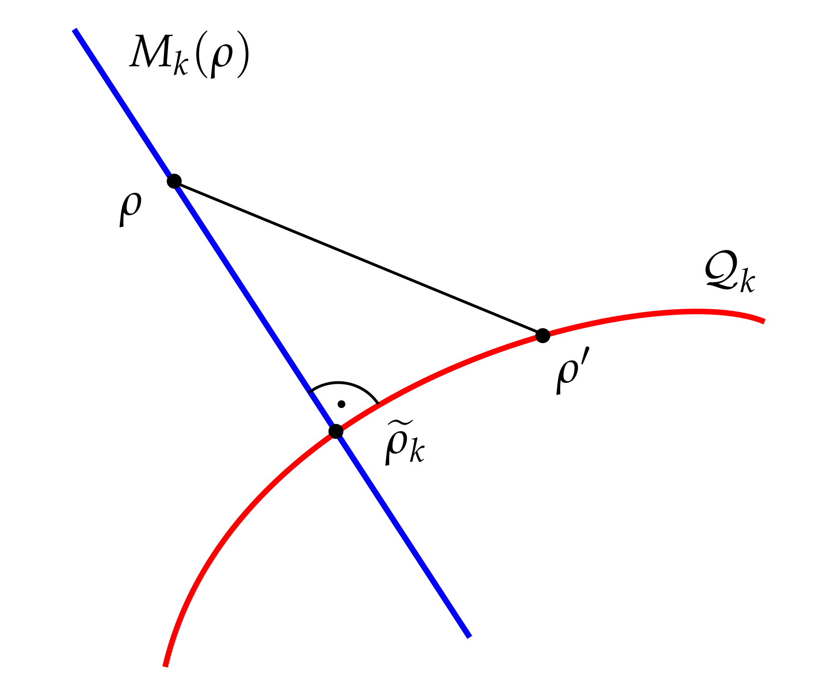
Figure 4: The information projection $\tilde{}\varrho_{k}$ of the state $\varrho$ is the closest state to $\varrho$ within the exponential family $\mathcal{Q}_{k}$. $M_{k}$ denotes the set of all quantum states that have the same $k$-body marginals as $\varrho$, and can also be used to characterize $\tilde{}\varrho_{k}$. For arbitrary states $\varrho^{\prime}$ within $\mathcal{Q}_{k}$ the relation $D(\varrho||\varrho^{\prime})=D(\varrho||\tilde{}\varrho_{k})+D(\tilde{}\varrho_{k}||\varrho^{\prime})$ holds, which resembles the Pythagorean Theorem. The figure is taken from Ref. [33]

4.2.2 Characterizing the approximation —

For the characterization of the information projection $\tilde{}\varrho_{k},$ the following result is quite helpful [31]. First, let $\varrho$ be an arbitrary quantum state, and $\tilde{}\varrho_{k}$ be the information projection onto the exponential family $\mathcal{Q}_{k}$. Furthermore, let $M_{k}$ be the set of all quantum states that have the same $k$-body marginals as $\varrho$. $M_{k}$ is, contrary to $\mathcal{Q}_{k}$, a linear subspace of the space of all density matrices (see Fig. 4). Then, the following statements are equivalent:

1. The state $\tilde{\varrho}_{k}$ is the closest state to $\varrho$ in $\mathcal{Q}_{k}$ with respect to the relative entropy.

2. The state $\tilde{\varrho}_{k}$ has the maximal entropy among all states in $M_{k}.$

3. The state $\tilde{\varrho}_{k}$ is the intersection $\mathcal{Q}_{k}\cap M_{k}.$

This equivalence can be used for many purposes. For example, it is useful for developing an algorithm for computing the information projection [34, 33]. Instead of minimizing the relative entropy as a highly nonlinear function over $\mathcal{Q}_{k}$, one can do the following: One optimizes over all states in $\mathcal{Q}_{k}$ with the aim to make the $k$-body marginals the same as for the state $\varrho$. The resulting algorithm converges well and allows the computation of the complexity measure $D_{k}$ for up to six qubits [33].

Second, from the equivalences it follows that the multi-information $D_{1}$ can directly be calculated, since the closest state to $\varrho$ in the family $\mathcal{Q}_{1}$ is the product state $\tilde{}\varrho_{1}=\varrho_{1}\otimes\varrho_{2}\otimes...\otimes\varrho_{N}$ built out of the reduced single-particle density matrices of $\varrho$. Clearly, $\tilde{}\varrho_{1}$ has the same marginals as $\varrho$ and maximizes the entropy.

4.2.3 A five-qubit example —

As a final example, let us discuss how the notion of exponential families can help to characterize ground states of two-body Hamiltonians. For that, consider the five-qubit ring-cluster state $|R_{5}\rangle.$ This state is defined to be the unique eigenstate fulfilling

$$|R_{5}\rangle=g_{i}|R_{5}\rangle,$$ (18)

where $g_{1}=\sigma_{x}\sigma_{z}\mathbb{1}\mathbb{1}\sigma_{z},g_{2}=\sigma_{z}\sigma_{x}\sigma_{z}\mathbb{1}\mathbb{1},g_{3}=\mathbb{1}\sigma_{z}\sigma_{x}\sigma_{z}\mathbb{1},g_{4}=\mathbb{1}\mathbb{1}\sigma_{z}\sigma_{x}\sigma_{z},$ and $g_{5}=\sigma_{z}\mathbb{1}\mathbb{1}\sigma_{z}\sigma_{x}.$ Here, the tensor product symbols have been omitted. After appropriate local transformations, the ring-cluster state can also be written as

$$|R_{5}\rangle=\frac{1}{\sqrt{8}}\big{[}|00000\rangle+|00110\rangle-|01011\rangle+|01101\rangle+|10001\rangle-|10111\rangle+|11010\rangle+|11100\rangle\big{]}.$$ (19)

The ring-cluster state is an example of a so-called graph state, and plays an important role in quantum error correction as a codeword of the five-qubit Shor code. It was known before that the state $|R_{5}\rangle$ cannot be the unique ground state of a two-body Hamiltonian [35]. This, however, leaves the question open whether it can be approximated by ground states of two-body Hamiltonians. For instance, for three qubits it was shown that not all pure states are ground states of two-body Hamiltonians, but all pure states can be approximated arbitrarily well by such ground states [36].

The characterization of the exponential families from the previous section can indeed help to prove that the state has $|R_{5}\rangle$ has finite distance to all thermal states of two-body Hamiltonians. For that, first note that the two-body marginals of the state $|R_{5}\rangle\!\langle R_{5}|$ are all maximally mixed two-qubit states. Then, one can directly find states which have the same two-body marginals, but their entropy is larger than the entropy the state $|R_{5}\rangle\!\langle R_{5}|$. This last property is, of course, not surprising, since $|R_{5}\rangle\!\langle R_{5}|$ has as a pure state the minimal possible entropy. According to the previous section, this already implies that $|R_{5}\rangle\!\langle R_{5}|$ cannot be the thermal or ground state of any two-body Hamiltonian.

Furthermore, if an arbitrary state $\varrho$ has a high fidelity with $|R_{5}\rangle$ then the two-body marginals will be close to the maximally mixed states, and in addition the entropy of $\varrho$ will be small. This implies that one can find again states with the same marginals and higher entropy. Using these ideas and some detailed calculations one can prove that if a state fulfils

$$F=\langle R_{5}|\varrho|R_{5}\rangle\geq\frac{31}{32}\approx 0.96875.$$ (20)

then it cannot be a thermal state of a two-body Hamiltonian [37]. This shows that the state $|R_{5}\rangle$ cannot be approximated by thermal states of two-body Hamiltonians. In principle, this bound can also be used to prove experimentally that a given state is not a thermal state of a two-body Hamiltonian.

5 Conclusion

In conclusion we have explained several problems occurring in the analysis of multiparticle quantum states, ranging from systematic errors of the measurement devices to the characterization of ground states of two-body Hamiltonians. We believe that several of the explained topics are important to be addressed in the future. First, since the current experiments in quantum optics are getting more and more complex, advanced statistical methods need to be applied in order to reach solid conclusions. Second, the analysis of ground states and thermal states of simple Hamiltonians is relevant for quantum simulation and quantum control, so direct characterizations would be very helpful.

6 Acknowledgements

We thank Rainer Blatt, Tobias Galla, Bastian Jungnitsch, Martin Hofmann, Lukas Knips, Thomas Monz, Sönke Niekamp, Daniel Richart, Philipp Schindler, Christian Schwemmer, and Harald Weinfurter for discussions and collaborations on the presented topics. Furthermore, we thank Mariami Gachechiladze, Felix Huber, and Nikolai Miklin for comments on the manuscript. This work has been supported by the EU (Marie Curie CIG 293993/ENFOQI, ERC Starting Grant GEDENTQOPT, ERC Consolidator Grant 683107/TempoQ), the FQXi Fund (Silicon Valley Community Foundation), and the DFG (Forschungsstipendium KL 2726/2-1).

References

References

- [1] R. Renner, Nature Physics 3, 645 (2007).
- [2] R. Horodecki, P. Horodecki, M. Horodecki, and K. Horodecki, Rev. Mod. Phys. 81, 865 (2009).
- [3] O. Gühne and G. Tóth, Phys. Rep. 474, 1 (2009).
- [4] T. Moroder, M. Keyl, and N. Lütkenhaus, J. Phys. A: Math. Theor. 41, 275302 (2008).
- [5] W. Hoeffding, J. Am. Stat. Assoc. 58, 301 (1963).
- [6] T. Moroder, M. Kleinmann, P. Schindler, T. Monz, O. Gühne, and R. Blatt, Phys. Rev. Lett. 110, 180401 (2013).
- [7] A. F. Mood, Introduction to the theory of statistics, McGraw-Hill Inc., 1974.
- [8] L. Schwarz and S. J. van Enk, Phys. Rev. Lett. 106, 180501 (2011).
- [9] N. K. Langford, New J. Phys. 15, 035003 (2013).
- [10] S. J. van Enk and R. Blume-Kohout, New J. Phys. 15, 025024 (2013).
- [11] C. Schwemmer, L. Knips, D. Richart, H. Weinfurter, T. Moroder, M. Kleinmann, and O. Gühne, Phys. Rev. Lett. 114, 080403 (2015).
- [12] Z. Hradil, Phys. Rev. A 55, 1561(R) (1997).
- [13] D. F. V. James, P. G. Kwiat, W. J. Munro, and A. G. White, Phys. Rev. A 64, 052312 (2001).
- [14] J. Shang, H. K. Ng, A. Sehrawat, X. Li, and B.-G. Englert, New J. Phys. 15, 123026 (2013).
- [15] M. Christandl and R. Renner, Phys. Rev. Lett. 109, 120403 (2012).
- [16] A. Peres, Phys. Rev. Lett. 77, 1413 (1996).
- [17] B. Jungnitsch, T. Moroder and O. Gühne, Phys. Rev. Lett. 106, 190502 (2011).
- [18] L. Vandenberghe and S. Boyd, SIAM Review 38, 49 (1996).
- [19] See the program PPTmixer, available at mathworks.com/matlabcentral/ fileexchange/30968.
- [20] L. Novo, T. Moroder, and O. Gühne, Phys. Rev. A 88, 012305 (2013).
- [21] X. Chen, P. Yu, L. Jiang, and M. Tian, Phys. Rev. A 87, 012322 (2013).
- [22] M. Hofmann, T. Moroder, and O. Gühne. J. Phys. A: Math. Theor. 47, 155301 (2014).
- [23] G. Tóth, T. Moroder, and O. Gühne. Phys. Rev. Lett. 114, 160501 (2015).
- [24] M. Huber and R. Sengupta, Phys. Rev. Lett. 113, 100501 (2014).
- [25] C. Lancien, O. Gühne, R. Sengupta, and M. Huber, J. Phys. A: Math. Theor. 48 505302 (2015).
- [26] S. Beigi and P. W. Shor, J. Math. Phys. 51, 042202 (2010).
- [27] T. Kahle, E. Olbrich, J. Jost and N. Ay, Phys. Rev. E 79, 026201 (2009).
- [28] S. Amari, IEEE Trans. Inf. Theory 47, 1701 (2001).
- [29] N. Ay and A. Knauf, Kybernetika 42, 517 (2007).
- [30] D. L. Zhou, Phys. Rev. Lett. 101, 180505 (2008).
- [31] D. L. Zhou, Phys. Rev. A 80, 022113 (2009).
- [32] T. Galla and O. Gühne, Phys. Rev. E 85, 046209 (2012).
- [33] S. Niekamp, T. Galla, M. Kleinmann, and O. Gühne, J. Phys. A: Math. Theor. 46, 125301 (2013).
- [34] D. L. Zhou, Commun. Theor. Phys. 61, 187 (2014).
- [35] M. Van den Nest, K. Luttmer, W. Dür, and H. J. Briegel, Phys. Rev. A 77, 012301 (2008).
- [36] N. Linden, S. Popescu, and W. K. Wootters, Phys. Rev. Lett. 89, 207901 (2002).
- [37] F. Huber and O. Gühne, Phys. Rev. Lett. 117, 010403 (2016).