Bayesian optimisation for fast approximate inference in state-space models with intractable likelihoods

Abstract

We consider the problem of approximate Bayesian parameter inference in non-linear state-space models with intractable likelihoods. Sequential Monte Carlo with approximate Bayesian computations (smc-abc) is one approach to approximate the likelihood in this type of models. However, such approximations can be noisy and computationally costly which hinders efficient implementations using standard methods based on optimisation and Monte Carlo. We propose a computationally efficient novel method based on the combination of Gaussian process optimisation and smc-abc to create a Laplace approximation of the intractable posterior. We exemplify the proposed algorithm for inference in stochastic volatility models with both synthetic and real-world data as well as for estimating the Value-at-Risk for two portfolios using a copula model. We document speed-ups of between one and two orders of magnitude compared to state-of-the-art algorithms for posterior inference.

Keywords: $\alpha$-stable distributions, approximate Bayesian computations, Bayesian inference, Gaussian process optimisation, sequential Monte Carlo

1 Introduction

Dynamical modelling of time series data is an essential part of many scientific fields including statistics (Durbin and Koopman, 2012), econometrics (McNeil et al., 2010) and engineering (Ljung, 1999). A popular dynamical model is the state-space model (ssm) which can be expressed by

$$x_{0}\sim\mu_{\theta}(x_{0}),\quad x_{t}|x_{t-1}\sim f_{\theta}(x_{t}|x_{t-1}),\qquad y_{t}|x_{t}\sim g_{\theta}(y_{t}|x_{t}),$$ (1)

where $\theta\in\Theta\subseteq\mathbb{R}^{p}$ denotes unknown static parameters. Here, $x_{t}\in\mathcal{X}\subseteq\mathbb{R}^{n_{x}}$ and $y_{t}\in\mathcal{Y}\subseteq\mathbb{R}^{n_{y}}$ denotes the latent state and the observations at time $t\in\{0,1,\ldots,T\}$, respectively. The distribution of the initial state, the state dynamics and the observations are modelled by using the known probability densities $\mu$, $f_{\theta}$ and $g_{theta}$, respectively.

In this paper, we are interested in estimating the unknown parameters $\theta$ in ssms using a Bayesian approach. This amounts to computing the parameter posterior distribution given by

$$p(\theta|y_{1:T})=\frac{p(\theta)p_{\theta}(y_{1:T})}{\displaystyle\int_{\Theta}\!p(\theta^{\prime})p_{\theta^{\prime}}(y_{1:T})\,\textrm{d}\theta^{\prime}},$$ (2)

where $p(\theta)$ and $p_{\theta}(y_{1:T})\triangleq p(y_{1},y_{2},\ldots,y_{T}|\theta)$ denote the parameter prior distribution and the likelihood, respectively. For an ssm, we cannot compute the posterior in closed-form due to that the likelihood $p_{\theta}(y_{1:T})$ depends on the unknown latent states $x_{0:T}$. Fortunately, it is possible to obtain unbiased estimates of the likelihood via so-called sequential Monte Carlo (smc; Doucet and Johansen, 2011) or particle filtering algorithms.

However for some models of interest, it is not possible to make use of smc due to that $g_{\theta}(y_{t}|x_{t})$ lacks an analytical closed-form expression, is defined recursively or is computationally prohibitive to evaluate. We refer to this class of models as ssms with intractable likelihoods. One example is when the $\alpha$-stable distribution (Nolan, 2003) is used as $g_{\theta}$ in (1) to model heavy-tailed noise in the observations. This type of modelling has recently been advocated by Stoyanov et al. (2010) among others to capture the behaviour of financial indices and stock prices, which often exhibit so-called jumps.

One approach to obtain a biased estimate of the intractable likelihood is to make use of approximate Bayesian computations (abc; Marin et al., 2012) in combination with smc (Jasra et al., 2012). The parameters $\theta$ can then be estimated using standard inference algorithms. However, the estimator obtained by smc-abc often suffers from a large variance and is computationally expensive to evaluate. This usually results in long run-times (days) of the complete inference algorithm, which is prohibitive in practical applications.

In this paper, we propose a computationally efficient algorithm for Bayes- ian inference in ssms with intractable likelihoods. The proposed algorithm is referred to as gsa and is a combination of Gaussian process optimisation (gpo; Brochu et al., 2010) and smc-abc. The aim of gsa is to construct a Laplace approximation to approximate (2). The efficiency of the proposed algorithm stems from that gpo requires substantially less posterior evaluations and is more robust to noise compared with other optimisation algorithms. This is mainly due to that gpo operates by constructing a surrogate function that mimics (2) in analogue with Wood (2010). The resulting surrogate is smooth and computationally cheap to evaluate, which enables the use of standard optimisation methods to extract a Laplace approximation of the surrogate mimicking the true posterior.

The main contribution of this paper is to introduce, develop and numerically study the gsa algorithm. We compare the proposed algorithm to particle Metropolis-Hastings (pmh; Andrieu et al., 2010; Dahlin and Schön, 2015) and spsa (Spall, 1998; Ehrlich et al., 2015) for inference in ssms using both synthetic and real-world data. In Bayesian inference, pmh is seen as the gold standard for posterior approximations and spsa is known as an efficient and scalable gradient-free optimisation algorithm. The numerical comparisons indicate that gsa can: (i) provide good posterior approximations, (ii) reduce the computational time by between one and two orders of magnitude compared with pmh, (iii) exhibit good robustness to the abc approximation and noise in the estimates. Furthermore, we demonstrate how to make use of the proposed algorithm in estimating the risk in financial portfolios.

Related work to the proposed algorithm is presented in e.g. Dahlin and Lindsten (2014), Gutmann and Corander (2016) and Meeds and Welling (2014). In the first two works, the authors aim to obtain a maximum likelihood estimate and map estimate using gpo, respectively. In the present work, we would like to approximate the entire posterior and not only the parameter that maximises the value of the likelihood or posterior. Moreover, compared with Meeds and Welling (2014), the uncertainty encoded into the surrogate function is utilized to determine the next point in which to sample the log-posterior.

We continue with Section 2, where an overview of the proposed algorithm and its components are presented. Sections 3 and 4 discuss the details of these components and the resulting algorithm is presented in Section 5. We conclude the paper with an extensive numerical evaluation in Section 6, and some remarks and future work in Section 7.

2 An intuitive overview of GSA

Our aim is to find Laplace approximation of the parameter posterior (2),

$$\widehat{p}(\theta|y_{1:T}) =\mathcal{N}\bigg{(}\theta;\widehat{\theta}_{\text{MAP}},\Big{[}\underbrace{-\nabla^{2}\log p(\theta|y_{1:T})\Big{|}_{\theta=\widehat{\theta}_{\text{MAP}}}}_{\triangleq\mathcal{J}(\widehat{\theta}_{\text{MAP}})}\Big{]}^{-1}\bigg{)},$$ (3)

where $\mathcal{N}(\theta;\mu,\Sigma)$ denotes the Gaussian distribution with mean $\mu$ and covariance matrix $\Sigma$. Here, $\mathcal{J}(\widehat{\theta}_{\text{MAP}})$ denotes the estimate of the Hessian of the log-posterior evaluated at the posterior mode,

$$\widehat{\theta}_{\text{MAP}}=\operatorname*{arg\!\max}_{\theta\in\Theta}\log p(\theta|y_{1:T}),$$ (4)

where $y_{1:T}$ denotes the recorded observations. This can be seen as a Gaussian approximation around the mode of the posterior motivated by the Bernstein-von Mises theorem, which states that the posterior concentrates to a Gaussian distribution centred at the true parameters with the inverse expected information matrix as its covariance when $T\rightarrow\infty$. Note that, even if this is an asymptotic results it can provide reasonable approximations using a finite number of samples as discussed by Panov and Spokoiny (2015).

We encounter two main problems when constructing the Laplace approximation: (i) the optimisation problem in (4) is difficult to solve efficiently and (ii) $\mathcal{J}(\widehat{\theta}_{\text{MAP}})$ is typically difficult to estimate with good accuracy. The first problem is due to the high variance in and computational cost of the posterior estimates. An example of this problem is presented in the left part of Figure 1. Here, we present the log-posterior estimates obtained by smc-abc over a grid of $\mu$ in (16). The high variance typically results in a slow convergence of parameter inference algorithms such as spsa and pmh. It is also difficult to speed up the convergence by using gradient information as this requires running computationally expensive particle smoothing algorithms.

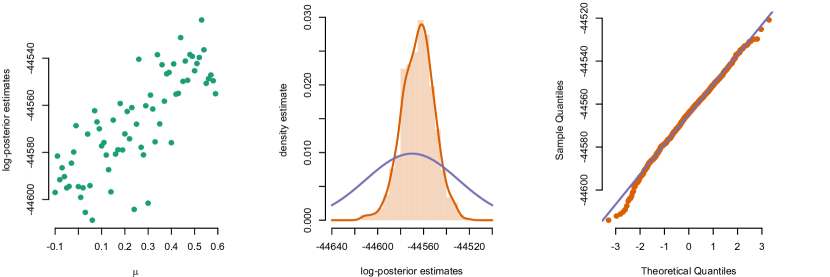
Figure 1: Samples from the log-posterior (left) of (16) with respect to $\mu$. The distribution (center) and qq-plot(right) of $1,000$ log-posterior estimates of (16). The purple lines indicate the best Gaussian approximation.

Instead, we propose to circumvent these problems by optimising a smooth surrogate function that mimics the log-posterior distribution similar to Wood (2010). We can then obtain a Laplace approximation using standard optimisation methods as the surrogate function is smooth and cheap to evaluate.

The surrogate function is obtained by gpo algorithm, which is a specific instance of Bayesian optimisation (Brochu et al., 2010). The surrogate function is sequentially updated using samples from the log-posterior. In this paper, we make use of the predictive distribution of a Gaussian process (gp) as the surrogate function. Hence, we can encode certain prior knowledge regarding the smoothness of the log-posterior into the gp prior, which reduces the number of samples required to explore the log-posterior.

The resulting gsa algorithm iterates three steps. At the $k$th iteration:

• compute an approximation of the log-posterior at the parameter $\theta_{k}$ denoted $\xi_{k}=\log\widehat{p}(\theta_{k}|y_{1:T})$ using smc-abc.

• construct a surrogate function by a gp predictive posterior using the observed data $\{\bm{\theta}_{k},\bm{\xi}_{k}\}=\{\theta_{j},\xi_{j}\}_{j=1}^{k}$.

• evaluate the acquisition rule to determine $\theta_{k+1}$.

The gpo algorithm then returns an estimate of the posterior and its uncertainty. There are two major advantages of gps for estimating the posterior density compared with e.g., using splines. Firstly, the uncertainty quantification can be used to develop so-called acquisition rules that explore areas with large uncertainty and exploits the information about the possible location of the mode of the posterior. This typically results in a rapid convergence of the algorithm, which limits the number of posterior samples required and hence also decreases the computational cost. Secondly, the gp can handle noisy function evaluations in a natural manner.

3 Estimating $\log p(\theta|y_{1:T})$

In this section, we discuss how to estimate the log-posterior that is required for carrying out Step (i) of gsa. This is done by making use of the (bootstrap) particle filter from which we can obtain an estimate of the marginal filtering distribution $p_{\theta}(x_{t}|y_{1:t})$ by

$$p^{N}_{\theta}(\textrm{d}x_{t}|y_{1:t})=\sum_{i=1}^{N}w_{t}^{(i)}\delta_{x_{t}^{(i)}}(\textrm{d}x_{t}),$$ (5)

where $x_{t}^{(i)}$ and $w_{t}^{(i)}$ denotes the particle $i$ at time $t$ and its normalised weight, respectively. Here, $\delta_{x}$ denotes the Dirac measure placed at $x$. As we shall see, the particle system $\{w_{t}^{(i)},x_{t}^{(i)}\}_{i=1}^{N}$ can also be used to obtain estimates of the log-posterior.

3.1 Particle filtering with ABC

The main problem with applying the particle filter is that it assumes that we can evaluate $g_{\theta}(y_{t}|x_{t})$ point-wise. In the current setting, this is not possible and instead we circumvent the evaluation of $g_{\theta}(y_{t}|x_{t})$ by using abc. This amounts to augmenting the posterior with an auxiliary variable $\check{y}_{1:T}$, which is data simulated from $g_{\theta}(y_{t}|x_{t})$ for $t=1,\ldots,T$. The fundamental assumption of abc is that data $\check{y}_{t}$ generated from $g_{\theta}(y_{t}|x_{t})$ should be similar to the observed data $y_{t}$ if $\theta$ is properly selected. The resulting augmented posterior can be expressed as

$$p_{\epsilon}(\theta,\check{y}_{1:T}|y_{1:T})=\frac{p(\theta)p_{\theta}\Big{(}\check{y}_{1:T}\Big{)}\rho\Big{(}\check{y}_{1:T};y_{1:T},\epsilon\Big{)}}{\displaystyle\int_{\Theta}\!p(\theta^{\prime})p_{\theta^{\prime}}\Big{(}\check{y}_{1:T}\Big{)}\rho\Big{(}\check{y}_{1:T};y_{1:T},\epsilon\Big{)}\,\textrm{d}\theta^{\prime}},$$

where, $\rho(\mu,\epsilon)$ denotes some density with mean $\mu$ and tolerance parameter $\epsilon$. This density is used to compute the distance between the simulated observations $\check{y}_{t}$ and the true observations $y_{t}$. A common choice is the Gaussian density $\rho(\mu,\epsilon)=\mathcal{N}(\mu,\epsilon^{2})$. Finally, we assume that the following marginalisation property holds

$$p_{\epsilon}(\theta|y_{1:T})=\int\!p_{\epsilon}(\theta,\check{y}_{1:T}|y_{1:T})\,\textrm{d}\check{y}_{1:T},$$

when the tolerance parameter is small enough and where $p_{\epsilon}(\theta|y_{1:T})$ denotes the posterior of the perturbed model. Hence, we recover a perturbed version of the posterior when $T\rightarrow\infty$ and $\epsilon$ is small enough.

To make use of this in the particle filter, we reformulate the ssm in (1) using abc as in Jasra et al. (2012). The observed data $y_{1:T}$ is perturbed by

$$\check{y}_{t}=\psi(y_{t})+z_{t},\quad z_{t}\sim\rho(0,\epsilon),$$ (6)

where $\psi$ denotes some suitable one-to-one transformation. Moreover, we assume that it is possible to simulate from the model using a transformation of random variables. This corresponds to that we can write $\check{y}_{t}=\tau_{\theta}(\check{x}_{t})$, where $\tau_{\theta}$ denotes a function of $\check{x}_{t}^{\top}=(x_{t}^{\top},v_{t}^{\top})$ and $v_{t}\sim\nu_{\theta}(v_{t}|x_{t})$ for some probability distribution $\nu_{\theta}$. This is a useful construction as it is often possible to generate samples from complicated distributions but not to evaluate them point-wise. See A for how to select $\tau_{\theta}$ and $\nu_{\theta}$ to generate $\alpha$-stable random variables.

From these two steps, we can rewrite the ssm (1) as

$$\check{x}_{t}|\check{x}_{t-1} \sim\Xi_{\theta}(\check{x}_{t}|\check{x}_{t-1})=\nu_{\theta}(v_{t}|x_{t})f_{\theta}(x_{t}|x_{t-1}),$$ (7a)

$$\check{y}_{t}|\check{x}_{t} \sim h_{\theta,\epsilon}(\check{y}_{t}|\check{x}_{t})=\rho\Big{(}\check{y}_{t};\psi(\tau_{\theta}(\check{x}_{t})),\epsilon\Big{)}.$$ (7b)

We can now apply a particle filter as in Algorithm 1 for this new model, which does not require us to evaluate the $g_{\theta}(y_{t}|x_{t})$ point-wise but only that we can simulate $\check{y}_{t}$. In this paper, we leave the choice of $\epsilon$ to the user, which can be done using e.g. pilot runs on simulated data. However, it is possible to adapt $\epsilon$ on-the-fly using the approaches discussed by e.g. Del Moral et al. (2012) or Calvet and Czellar (2015). However in our experience, these methods require a larger value of $N$ than un-adapted smc-abc to provide log-posterior estimates with a reasonable bias. Therefore, we decided to fix $\epsilon$ in this paper to obtain computationally efficient algorithms.

Algorithm 1 Estimate the log-posterior by particle filtering

Inputs: $\check{y}_{1:T}$ (perturbed data), ssm (7), $N\in\mathbb{N}$ (no. particles), $\rho_{\epsilon}$ (density for abc approximation) with $\epsilon\in\mathbb{R}_{+}$ (tolerance par.).
Outputs: $\log\widehat{p}^{N}(\theta|\check{y}_{1:T})$ (est. of log-posterior).
Note: all operations are carried out over $i,j=1,\ldots,N$.

 

1:  Sample $\check{x}^{(i)}_{0}\sim\mu_{\theta}(x_{0})\nu_{\theta}(v_{0}|x_{0})$ and set $w_{0}^{(i)}=1/N$.

2:  for $t=1$ to $T$ do

3:     Apply systematic resampling to obtain the ancestor index $a^{(i)}_{t}$ from a categorical distribution with $\mathbb{P}\Big{(}a^{(i)}_{t}=j\Big{)}=w^{(j)}_{t-1}.$

4:     Propagate particles using $\check{x}^{(i)}_{t}\sim\Xi_{\theta}\Big{(}\check{x}_{t}|\check{x}_{t-1}^{a_{t}^{(i)}}\Big{)}$ and set $\check{x}_{0:t}^{(i)}=\Big{\{}\check{x}_{0:t-1}^{a_{t}^{(i)}},\check{x}_{t}^{(i)}\Big{\}}$.

5:     Compute particle weights by $W_{t}^{(i)}=h_{\theta,\epsilon}\Big{(}\check{y}_{t}|\check{x}_{t}^{(i)}\Big{)}$ and $w^{(i)}_{t}=W_{t}^{(i)}\left[\sum_{j=1}^{N}W_{t}^{(j)}\right]^{-1}.$

6:  end for

7:  Compute $\log\widehat{p}^{N}(\theta|\check{y}_{1:T})$ by (8).

3.2 The estimator and its statistical properties

An estimator for the log-posterior of the perturbed model (7) is given by

$$\log\widehat{p}^{N}(\theta|y_{1:T}) =\log\widehat{p}^{N}_{\theta}(y_{1:T})+\log p(\theta)$$

$$=\sum_{t=1}^{T}\log\left\{\sum_{i=1}^{N}W_{t}^{(i)}\right\}-T\log N+\log p(\theta),$$ (8)

which makes use of the unnormalised weights generated by Algorithm 1. It is known from Pitt et al. (2012) that the estimator (8) is biased for a finite number of particles but it is consistent and asymptotically Gaussian. Specifically, we have that the error in the log-posterior estimate fulfils a clt given by

$$\sqrt{N}\bigg{[}\log p(\theta|y_{1:T})-\log\widehat{p}^{N}(\theta|y_{1:T})+\frac{\gamma^{2}(\theta)}{2N}\bigg{]}\stackrel{{\scriptstyle d}}{{\longrightarrow}}\mathcal{N}\Big{(}0,\gamma^{2}(\theta)\Big{)},$$ (9)

when $N\rightarrow\infty$ and for some unknown variance $\gamma(\theta)$. As a result, we have an expression for the bias of the estimator given by $-\gamma^{2}(\theta)/2N$ for a finite number of particles. However, we see that the error is approximately Gaussian for this type of model in the finite sample case by the experimental data presented in the center and right parts of Figure 1.

The log-posterior estimator in (8) is consistent with respect to the perturbed model (7) but not the true model (1). Dean and Singh (2011) show that the perturbation results in a bias in the parameter estimates (w.r.t. the unperturbed model) that decrease proportional to $\mathcal{O}(\epsilon^{2})$ under some regularity assumptions. Furthermore, the asymptotic Gaussianity of the estimator and a Bernstein-von Mises-type theorem holds for a small enough $\epsilon$. This is an important fact to motivate the Laplace approximation as discussed in Section 2 and we investigate these properties empirically in Section 6.1.

4 Constructing the surrogate of $\log p(\theta|y_{1:T})$

In this section, we briefly discuss Steps (ii) and (iii) of gsa, where we construct a surrogate function to mimic the log-posterior. The interested reader is referred to Brochu et al. (2010) for more details.

4.1 Gaussian process prior

gps (Rasmussen and Williams, 2006) are an instance of so-called Bayesian non-parametric models and can be interpreted as a generalisation of the multivariate Gaussian distribution to an infinite dimensional setting. A realisation drawn from a gp can therefore be seen as an infinite vector of real values (a function over the real space $\mathbb{R}^{p}$). To construct the surrogate function, we assume a priori that the log-posterior is distributed according to

$$\log p(\theta|y_{1:T})\sim\mathcal{GP}\big{(}m(\theta),\kappa(\theta,\theta^{\prime})\big{)}.$$ (10)

Note that this does not correspond to an assumption that the log-posterior of the parameters in the ssm is Gaussian. Here, $\mathcal{GP}(m,\kappa)$ denotes a gp with mean function $m$ and covariance function $\kappa$ defined by

$$m(\theta) =\mathbb{E}\Big{[}\log p(\theta|y_{1:T})\Big{]},$$

$$\kappa(\theta,\theta^{\prime}) =\mathbb{E}\Big{[}\Big{(}\log p(\theta|y_{1:T})-m(\theta)\Big{)}\Big{(}\log p(\theta^{\prime}|y_{1:T})-m(\theta^{\prime})\Big{)}\Big{]}.$$

The mean function specifies the expected value of the process and the covariance function specifies the dependence between any pair of points on the log-posterior function. The covariance function depends on a set of hyperparameters, such as the length scale that controls the dependence, see Rasmussen and Williams (2006) for details. From the clt in (9) and Figure 1, we know that the error in the log-posterior is approximately Gaussian,

$$\xi_{k}=\log\widehat{p}^{N}(\theta_{k}|y_{1:T})\approx\log p(\theta_{k}|y_{1:T})+\sigma_{\xi}z_{k},\qquad z_{k}\sim\mathcal{N}(0,1),$$ (11)

where $\sigma^{2}_{\xi}$ denotes some unknown variance estimated in a later stage of the algorithm. Consequently, we have that the predictive posterior for any test point $\theta_{\star}\in\Theta$ is given by

$$\log p(\theta_{\star}|y_{1:T})|\mathcal{D}_{k} \sim\mathcal{GP}\Big{(}\mu(\theta_{\star}|\mathcal{D}_{k}),\sigma^{2}(\theta_{\star}|\mathcal{D}_{k})+\sigma^{2}_{\xi}\Big{)},$$ (12a)

$$\mu(\theta_{\star}|\mathcal{D}_{k}) =m(\theta_{\star})$$

$$+\kappa(\theta_{\star},\bm{\theta}_{k})\Big{[}\kappa(\bm{\theta}_{k},\bm{\theta}_{k})+\sigma^{2}_{\xi}\mathbf{I}_{k\times k}\Big{]}^{-1}\Big{\{}\bm{\xi}_{k}-m(\theta_{\star})\Big{\}},$$ (12b)

$$\sigma^{2}(\theta_{\star}|\mathcal{D}_{k}) =\kappa(\theta_{\star},\theta_{\star})$$

$$-\kappa(\theta_{\star},\bm{\theta}_{k})\Big{[}\kappa(\bm{\theta}_{k},\bm{\theta}_{k})+\sigma^{2}_{\xi}\mathbf{I}_{k\times k}\Big{]}^{-1}\kappa(\bm{\theta}_{k},\theta_{\star}),$$ (12c)

where we have introduced the notation $\mathcal{D}_{k}=\{\bm{\theta}_{k},\bm{\xi}_{k}\}$ for the information available at iteration $k$. The surrogate function of the log-posterior is then given by (12). The major cost in computing the predictive posterior is incurred by the matrix inversion which is proportional to $\mathcal{O}(k^{3})$. Hence, sparse formulations of the gp can be useful to decrease the computation cost for large $K$, see Rasmussen and Williams (2006).

4.2 Acquisition function

The surrogate function given by the gp predictive distribution gives us the estimate of the log-posterior and its uncertainty. As previously mentioned, this is useful information for creating an acquisition rule $\mathsf{AQ}(\theta_{\star}|\mathcal{D}_{k})$ to balance exploration and exploitation. We can then determine the next point in which to sample the log-posterior by

$$\theta_{k+1}=\operatorname*{arg\!\max}_{\theta_{\star}\in\Theta_{\text{GPO}}}\mathsf{AQ}(\theta_{\star}|\mathcal{D}_{k}),$$

where $\Theta_{\text{GPO}}$ denotes a search space defined by the user. In this paper, we make use of the expected improvement (ei) due to its general good performance in numerical evaluations (Lizotte, 2008). To derive the ei rule, consider the predicted improvement defined as

$$\mathsf{PI}(\theta_{\star}) =\max\Big{\{}0,\log p(\theta_{\star}|y_{1:T})-\mu_{\max}-\zeta\Big{\}},\qquad\forall\theta_{\star}\in\Theta_{\text{GPO}},$$ (13)

where $\mu_{\max}$ denotes the maximum value of $\mu(\theta)$ for the sampled points $\theta\in\bm{\theta}_{k}$. Here, we introduce $\zeta$ as a parameter that controls the exploitation/exploration behaviour as in Lizotte (2008). Hence for $\zeta=0$, we have that $\mathsf{PI}(\theta_{\star})$ is the difference between the posterior and the maximum value it assumes in the set of sampled points. Therefore, it is positive for points where the log-posterior is larger than the current peak and zero for all other points. The ei rule is obtained by computing the expected value of (13) with respect to (12). This results in the acquisition rule given by

$$\theta_{k+1} =\left\{\operatorname*{arg\!\max}_{\theta_{\star}\in\Theta_{\text{GPO}}}\,\sigma(\theta_{\star}|\mathcal{D}_{k})\Big{[}Z(\theta_{\star})\Phi\big{(}Z(\theta_{\star})\big{)}+\phi\big{(}Z(\theta_{\star})\big{)}\Big{]}\right\}+\check{z}_{k},$$ (14)

$$Z(\theta_{\star}) =\sigma^{-1}(\theta_{\star}|\mathcal{D}_{k})\Big{[}\mu(\theta_{\star}|\mathcal{D}_{k})-\mu_{\max}-\zeta\Big{]},$$

where $\phi$ and $\Phi$ denotes the density and distribution function of the standard Gaussian distribution, respectively. Here, we jitter to the solution of the optimisation problem by adding Gaussian noise $\check{z}_{k}\sim\mathcal{N}(0,\Sigma)$ with covariance $\Sigma$. In practice, this improves the exploration and increases the accuracy of the obtained parameter estimates. Jittering is also advocated by Bull (2011) and Gutmann and Corander (2016) to increase the convergence rate of gpo.

The optimisation in (14) is possibly non-convex but it is cheap to evaluate the objective function as it only amounts to evaluating the gp predictive posterior in one point. We make use of the the gradient-free dividing rectangles (direct; Jones et al., 1993) to solve (14) over $\Theta_{\text{GPO}}$, which is determined from the support of the prior distribution $p(\theta)$.

5 The GSA algorithm

gsa (Algorithm 2) is obtained by combining smc-abc (Algorithm 1) to approximate the log-posterior point-wise and gpo to create a surrogate function that mimics the log-posterior around its mode. In this section, we discuss some user choices and convergence results for the algorithm. See A for the details of the implementation employed in this paper.

5.1 Initialisation and convergence criteria

We initialise Algorithm 2 at Line 1 to find some suitable hyperparameters for the gp prior. The hyperparameters are estimated using $L$ initial samples from the log-posterior obtained by Latin hypercube sampling. We then execute Algorithm 1 for each of the sampled parameters $\{\theta_{1}^{\star},\theta_{2}^{\star},\ldots,\theta_{L}^{\star}\}$ to obtain $\mathcal{D}^{\star}_{L}$ by the analogue of Line 4 in Algorithm 2. After the initialisation of the algorithm, we can update the hyperparameters with Line 5 at every iteration or at some pre-defined interval. Estimating the hyperparameters is computationally costly and it is therefore recommended to re-estimate them only at some fixed interval. The algorithm is usually executed for some pre-defined number of iterations $K$ or until the ei is smaller than some $\Delta\mathsf{EI}>0$, i.e. until $k$ satisfies $\mathsf{EI}(\theta_{k}|\mathcal{D})<\Delta\mathsf{EI}$.

Algorithm 2 Find a Laplace approximation of $\log p(\theta|y_{1:T})$ using GSA

Inputs: Algorithm 1, $p(\theta)$ (parameter prior), $m(\theta)$ (mean function), $\kappa(\theta,\theta^{\prime})$ (covariance function), $\theta_{1}$ (initial parameter), $\Sigma$ (jittering covariance) and $\Theta_{\text{GPO}}$ (optimisation bounds).
Output: $\widehat{\theta}_{\text{MAP}}$ (est. of the parameter) and $\widehat{\mathcal{J}}(\widehat{\theta}_{\text{MAP}})$ (est. of posterior covariance).

 

1:  Estimate the hyperparameters of the gp prior by using some initial data $\mathcal{D}^{\star}_{L}$.

2:  Initialise the parameter to $\theta_{1}$ and set $k=1$.

3:  while convergence criteria is not satisfied do

4:     Estimate $\xi_{k}=\log\widehat{p}(\theta_{k}|y_{1:T})$ by Algorithm 1 and set $\mathcal{D}_{k}=\{\mathcal{D}^{\star}_{L},\bm{\theta}_{k},\bm{\xi}_{k}\}$.

5:     (if required) Update the hyperparameters of the gp prior using $\mathcal{D}_{k}$.

6:     Construct the gp surrogate $\log p(\theta_{\star}|y_{1:T})|\mathcal{D}_{k}$ using (12).

7:     Compute $\mu_{\max}=\operatorname*{arg\!\max}_{\theta\in\bm{\theta}_{k}}\mu(\theta|\mathcal{D}_{k})$.

8:     Compute $\theta_{k+1}$ by (14) using optimisation over $\Theta_{\text{GPO}}$.

9:     Set $k=k+1$.

10:  end while

11:  Compute the map estimate $\widehat{\theta}$ by optimising $\mu(\theta|\mathcal{D}_{k})$ using optimisation over $\Theta_{\text{GPO}}$.

12:  Extract the Hessian estimate $\mathcal{J}(\widehat{\theta}_{\text{MAP}})$ using e.g. finite-differences on $\mu(\theta|\mathcal{D}_{k})$.

5.2 Extracting the Laplace approximation

From Algorithm 2, we obtain the predictive posterior mean function $\mu(\theta_{\star}|\mathcal{D})$, which hopefully is an accurate surrogate for the log-posterior. We then proceed to extract the map estimate $\widehat{\theta}_{\text{MAP}}$ defined by (4). As the surrogate is smooth and cheap to evaluate, we can carry out the optimisation using standard methods such as the direct algorithm to find the mode. The estimate of the Hessian of the log-posterior $\mathcal{J}(\widehat{\theta}_{\text{MAP}})$ can be computed by a finite-difference scheme, by analytically computing the Hessian of $\mu(\theta_{\star}|\mathcal{D})$ when possible or by using a quasi-Newton algorithm to solve (4).

5.3 Convergence properties

There are only a limited number of results regarding the convergence properties of the gpo algorithm in the literature. Most of the properties have been studied numerically by benchmarking the gpo algorithm against alternatives on a large number of optimisation problems. However, some theoretical results are discussed by Bull (2011) and Vazquez and Bect (2010). They conclude that gpo using the ei rule samples the log-posterior densely if it is continuous with respect to the gp prior. Also, gpo achieves an optimal convergence rate of the order $\mathcal{O}\big{(}(K\log K)^{-5/p}(\log K)^{1/2}\big{)}$ for the Matérn 5/2 covariance function, where $K$ and $p$ denote the number of samples and parameters to infer, respectively.

6 Numerical illustrations and applications

In this section, we provide four illustrations of the properties and advantages of the proposed algorithm. The implementation details are collected in A and the source code with data is available for download at GitHub: https://github.com/compops/gpo-smc-abc/.

6.1 Stochastic volatility with Gaussian log-returns

Consider the stochastic volatility model with Gaussian log-returns (gsv),

$$x_{0} \sim\mathcal{N}\left(x_{0};\mu,\frac{\sigma^{2}_{v}}{\big{(}1-\phi^{2}\big{)}}\right),$$ (15a)

$$x_{t+1} \sim\mathcal{N}\Big{(}x_{t+1};\mu+\phi(x_{t}-\mu),\sigma_{v}^{2}\Big{)},$$ (15b)

$$y_{t} \sim\mathcal{N}\Big{(}y_{t};0,\exp(x_{t})\Big{)},$$ (15c)

with parameters $\theta=\{\mu,\phi,\sigma_{v}\}$. Here, the latent log-volatility is assumed to follow a mean-reverting random walk with mean $\mu\in\mathbb{R}$, persistence $\phi\in(-1,1)$ and standard deviation of the increments $\sigma_{v}\in\mathbb{R}_{+}$. We generate a single synthetic data set from this model with $T=500$ observations, parameters $\theta^{\star}=\{0.20,0.96,0.15\}$ and initial state $x_{0}=0$.

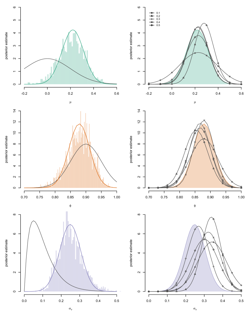
Figure 2: Marginal parameter posteriors for the synthetic data in the gsv model. Left: Solid curves indicate the Laplace approximations of the posterior using gs for $\mu$ (green), $\phi$ (orange) and $\sigma_{v}$ (purple). The histograms represent the exact posteriors estimated using pmh and the dark grey (left) curves indicate the prior distributions. Right: Laplace approximations (shaded areas) from gs for the three parameters. The grey curves (right) indicate the Laplace approximations obtained by gsa using five different values of the tolerance parameter $\epsilon$ in the abc approximation.

This model is interesting since it allows us to compare the gsa algorithm to an algorithm that makes use of a standard particle filter to estimate the log-posterior. This is possible as we can evaluate $g_{\theta}(y_{t}|x_{t})$ in closed-form for (15). We refer to this version of the algorithm as gs and it corresponds to the gsa algorithm with tolerance parameter $\epsilon=0$.

In the left part of Figure 2, we present the posterior estimates from gs (solid curve) and pmh (histogram). We begin by observing a good fit of the Laplace approximation from gs to the histogram approximation obtained by pmh; both the location and the spread of the posterior approximations are similar. Using gs results in a speed-up of about $30$ times ($15,000/500\approx 30$) compared with pmh, where the latter is seen as the gold standard in computational Bayesian inference The main computational cost for both algorithms is incurred by running the particle filter (one run per iteration). The overhead for the proposed algorithm (estimating hyperparameters in the gp and computing the predictive posterior) is negligible compared with the computational cost of running a particle filter.

We now continue with analysing the Laplace approximations obtained by gsa. In the right side of Figure 2, we present the posterior approximations obtained by varying the tolerance parameter $\epsilon$ between $0.1$ and $0.5$ to study the bias and robustness of the approximation. Darker shades of grey indicate a larger tolerance parameter. For $\epsilon=0.1$ and $0.2$, we see that the approximations are rather poor with a significant bias and bad fit to the spread. However for the other choices of $\epsilon$, the approximations from gsa converges quickly to be similar to gs (solid curve). From these results, we conclude that there is a bias in the posterior approximation when $\epsilon$ is too small and the approximation tends to grow wider as $\epsilon$ increases. Hence, a bias-variance trade-off is introduced into the posterior approximation depending on $\epsilon$.

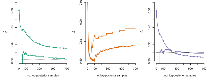
Figure 3: The trace of the map estimate for $\mu$ (green), $\phi$ (orange) and $\sigma_{v}$ (purple) from gs (solid) and spsa (solid-cicle) as a function of the number of log-posterior samples. The first $L=50$ samples of gs are used to estimate the hyperparameters. Both algorithms are run for a total of $700$ log-posterior samples. Dashed lines indicate the posterior means from pmh.

We continue by comparing gs to spsa, where the latter is a gradient-free alternative with good convergence properties and performance in many applications. spsa operates by constructing a finite-difference approximation of the gradient at each iteration after which it takes a step in the gradient direction. Note that spsa requires two log-posterior estimates at each iteration compared with only one sample in the gs. Another possible drawback with spsa is that it only provides the map estimate and no quantification of the posterior uncertainty.

In Figure 3, we compare the map parameter estimates of two algorithms as a function of the number of log-posterior estimates. The first $L=50$ samples of the log-posterior are used to estimate the hyperparameters of the gp prior. After this initial phase, gs converges quickly to reasonable values of the parameters using about half the number of posterior samples. This results in a speed-up of factor $2$ when using the proposed algorithm compared with spsa.

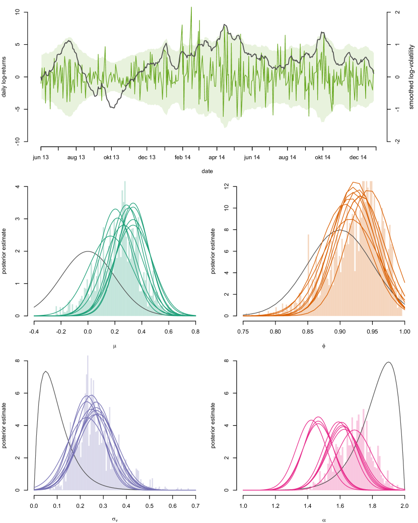
Figure 4: Upper: log-returns (green) of coffee futures and the estimate of the log-volatility (dark grey). The shaded area indicates the $95\%$ confidence region for the log-returns according to the $\alpha$sv model. Middle and lower: marginal parameter posteriors in the $\alpha$sv model estimated by gsa (solid curves) using $10$ independent runs and pmh (histogram) for $\mu$ (green), $\phi$ (orange), $\sigma_{v}$ (purple) and $\alpha$ (magenta). Dark grey curves indicate the prior distributions.

6.2 Stochastic volatility model $\alpha$-stable log-returns

In the upper part of Figure 4, we present the log-returns of future contracts on coffee during the period between June, 2013 and December, 2014. The data seem to indicate the presence of jumps around the first half of $2014$. This is common in financial data and can be modelled in a number of different ways. To this end, we consider the stochastic volatility model with $\alpha$-stable log-returns ($\alpha$sv) given by

$$x_{0} \sim\mathcal{N}\left(x_{0};\mu,\frac{\sigma^{2}_{v}}{\big{(}1-\phi^{2}\big{)}}\right),$$ (16a)

$$x_{t+1} \sim\mathcal{N}\Big{(}x_{t+1};\mu+\phi(x_{t}-\mu),\sigma_{v}^{2}\Big{)},$$ (16b)

$$y_{t} \sim\mathcal{A}\Big{(}y_{t};\alpha,\exp(x_{t})\Big{)},$$ (16c)

with parameters $\theta=\{\mu,\phi,\sigma_{v},\alpha\}$ and $\mathcal{A}(\alpha,\gamma)$ denoting a zero-mean symmetric $\alpha$-stable distribution with stability parameter $\alpha\in(0,2)$ and scale $\gamma\in\mathbb{R}_{+}$. The stability parameter determines the tail behaviour of the distribution, see Nolan (2003) for a discussion of the $\alpha$-stable distribution and its properties. The likelihood is in general intractable for this model and therefore approximations such as the particle filtering using abc are required.

In the middle and lower part of Figure 4, we compare the posterior approximations obtained with gsa (solid curves) with $10$ independent runs and pmh (histograms). We see that the mixing of pmh is quite poor for this model as the histograms are peaky. This is a common problem as Markov chains tends to get stuck if the log-posterior estimates are noisy. However, the posterior estimates overlap and seems to give reasonable parameter values for each run of gsa. The main difference is in the estimate of $\alpha$, which could be the result of the abc approximation or problems with observability. Finally, the estimate the log-volatility (black) seems reasonable when compared to the log-returns.

6.3 Computing VaR for a portfolio of oil futures

We follow Charpentier (2015) to construct a copula model to capture the dependency structure between prices of oil future contracts. The data considered is presented in Figure 5 and consists of weekly log-returns between January 10, 1997 and June 4, 2010 of Brent (produced in the North Sea), Dubai (produced in the Persian Gulf) and Maya (produced in the Gulf of Mexico) oil. We partition the data set into two parts and make use of the first $465$ data points for estimating the $\alpha$sv and copula models. The remaining $233$ data points are kept for validating the model by backtesting.

Algorithm 3 Copula modelling using $\alpha$sv as the marginal models

Stage 1 (repeated for each asset $i$)

1:  Run Algorithm 2 to obtain the log-volatility estimate $\widehat{x}_{1:T,i}$ and the parameter estimate $\widehat{\theta}_{\text{MAP},i}$ of (16). Compute the filtered log-returns $\widehat{e}_{t,i}$ by

$$\widehat{e}_{t,i}=\exp\bigg{(}-\frac{1}{2}\widehat{x}_{t,i}\bigg{)}y_{t},\qquad\text{ for }t=1,\ldots,T.$$ (17)

2:  Estimate the cumulative distribution function (cdf) denoted by $\widehat{G}_{i}$ from $\{\widehat{e}_{t,i}\}_{t=1}^{T}$. Compute the probability transformation of the residuals by

$$\widehat{u}_{t,i}=\widehat{G}_{i}(\widehat{e}_{t,i}),\qquad\text{ for }t=1,\ldots,T.$$ (18)

Stage 2

4:  Infer the parameters of the copula to model the dependency between $\{\{\widehat{u}_{t,i}\}_{t=1}^{T}\}_{i=1}^{30}$.

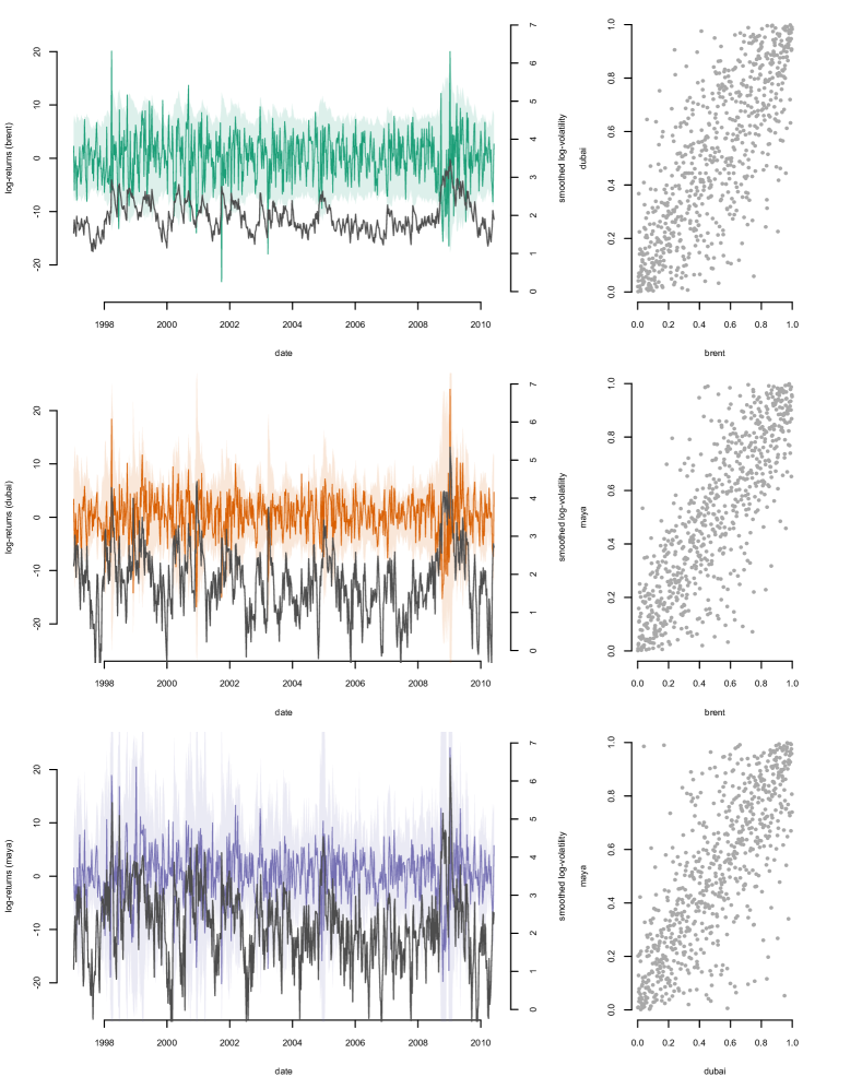
Figure 5: Left: weekly log-returns of Brent (green), Dubai (orange) and Maya (purple) oil between January 10, 1997 and June 4, 2010. The shaded area indicates the $95\%$ confidence region for the log-returns according to the $\alpha$sv model. The dark grey curves indicate estimates of the log-volatility. Right: the corresponding transformed filtered residuals $\widehat{u}_{t,i}$.

We adopt the commonly used two-stage approach to copula modelling outlined in Algorithm 3, where marginal models are first fitted separately to each of the log-return series, and then combined using a copula to model the dependency structure (Joe, 2005). We make use of the procedure in Section 6.2 to estimate the parameters of an $\alpha$sv model for each type of oil. The filtered residuals (17) are assumed to be independent and identically distributed as $\mathcal{A}(\widehat{\alpha}_{i},1)$ by (16) if $x_{1:T}$ is known. Stage 1 is carried out independently for each asset and is therefore straight-forward to implemented in a parallel manner. The use of the proposed algorithm decreases the computational time for this stage from hours or days for each asset to about half an hour compared with pmh.

We follow McNeil et al. (2010, p. 231-231) to model the dependency in the residuals. This amounts to applying a probability transform via the empirical cdf on the residuals into the $3$-dimensional hypercube, see right part of Figure 5. The transformed residuals $\{\widehat{u}_{1:T,1},\ldots,\widehat{u}_{1:T,d}\}$ are then combined by a Student’s $t$-copula function to find a model for the joint distribution. The degrees of freedom and the correlation matrix in the Student’s $t$-copula are estimated using map and matching of moments via Kendall’s $\tau$, respectively.

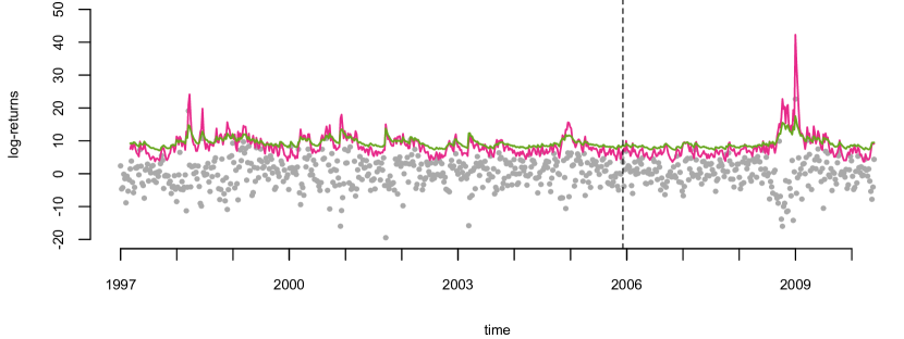
Figure 6: Estimated values of $\mathsf{VaR}_{0.99}(e_{t})$ for an equally weighted portfolio of the three oil futures using the gsv (magenta) and $\alpha$sv (green) model with the Student-$t$ copula. The dashed line indicates the division of estimation and validation data.

Finally, we make use of the copula models and their margins to estimate the var for each type of oil. The var at confidence $\bar{\alpha}\in(0,1)$ is defined by

$$\mathsf{VaR}_{\bar{\alpha}}(e_{t})=\inf\Big{\{}-e_{t}\in\mathbb{R}:G(-e_{t})\geq\bar{\alpha}\Big{\}},$$

i.e. the smallest loss $-e_{t}$ such that probability that the loss (the negative log-return) exceeds $-e_{t}$ is no larger then $(1-\bar{\alpha})$. We adopt a Monte Carlo approach to estimate $\mathsf{VaR}_{\bar{\alpha}}(e_{t})$ by: (i) simulating from the copula, (ii) obtain simulated filtered residuals by applying a quantile transform based on the empirical cdf, (iii) computing the resulting log-returns by the estimated volatility and the inverse of (17). We repeat this $100,000$ times for each asset and then compute the empirical quantile corresponding to $\mathsf{VaR}_{0.99}(e_{t})$ for an equally weighted portfolio. However, more advanced portfolio weighting schemes can be easily implemented.

The resulting var-estimate is presented Figure 6, where we compared the $\alpha$sv model with a gsv model (15) estimated using gs in a similar manner. We note that the estimates from the two models are quite different especially at the end of the data series. Backtesting on the validation data gives $0$ violations for both models and the expected number of violations is $2.3$. The gsa algorithm requires around $30-60$ minutes to infer the model for each of the three assets, where the inference is straight-forward to run on parallel architecture. The corresponding computational time required by the pmh algorithm would be in the order of $18-24$ hours.

6.4 Computing VAR for a portfolio of stocks

We offer a final numerical example to illustrate that the proposed method can be applied to large portfolios as well. The data that we consider is the 30 industrial portfolio provided by Kenneth French. The portfolio consists of monthly log-returns of $30$ different industrial sectors during the period September, 1926 to December, 2015. Again, we partition the data into an estimation set and a validation set with $716$ and $358$ data points, respectively.

We adopt the same procedure as in Section 6.3 and the results are presented in Figure 7. The conclusions are similar with both var estimates being quite similar. Backtesting gives $0$ and $1$ violations for the $\alpha$sv and gsv models, respectively. The expected number of violations is $3.5$. The computational speed-up with gsa compared with pmh is similar to in Section 6.3 as the number of observations per asset are similar.

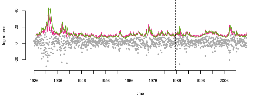
Figure 7: The log-returns (grey dots) and the estimated values of $\mathsf{VaR}_{0.99}(e_{t})$ for an equally weighted portfolio of stocks using the gsv (magenta) and $\alpha$sv (green) model with the Student’s $t$-copula. The dashed line indicates the division of estimation and validation data.

7 Conclusions

We have proposed gsa, an algorithm to approximate the posterior distribution in ssms with intractable likelihoods. The illustrations provided in Section 6 indicate that the proposed algorithm is quite accurate and exhibits a substantial decrease in the computational cost. We obtain similar posterior estimates to pmh with a speed-up of one or two orders of magnitude, which reduces computational time from tens of hours to tens of minutes. Moreover, gsa seems to be quite robust to noise in the log-posterior estimates, which typically results in that the pmh algorithm gets stuck at times and that the spsa algorithm converges slowly. Overall, this shows that the proposed algorithm is an efficient inference method that makes it possible for practitioners to use models with intractable likelihoods, such as copula models with $\alpha$-stable margins, in applied work.

Future work includes: (i) adopting a sparse representation of the gp, (ii) developing new acqusition functions, (iii) making use of better tailored covariance functions and (iv) incorperating adaptive approaches for choosing the tolerance level $\epsilon$. Some ideas for sequential and sparse representations of gps are discussed by Huber (2014) and Bijl et al. (2015). It would also be interesting to design new acquisition functions to obtain good estimates of the Hessian of the log-posterior or higher order moments at the same time as the map estimate. This could improve the Laplace approximation of the parameter posterior and open up for alternative posterior approximations such as using the skewed Student’s $t$-distribution. Moreover, an interesting approach for tailored gp priors would be to make use of non-stationary covariance functions (Paciorek and Schervish, 2004). This would capture the fact that the log-posterior often falls off rapidly in some parts of the parameter space and is almost flat in other parts.

Finally, it would be beneficial to include some adaptive approach to select $\epsilon$ in the smc-abc algorithm to decrease the number of choices for the user. As previously discussed, we initially implemented the adaptive algorithms proposed in Del Moral et al. (2012) and Calvet and Czellar (2015). However, we ran into problems when using them to approximate the log-posterior values using moderate values of $N$. The estimates exhibited a large bias that resulted in biased estimates of $\theta$ using pmh. As a result, we choose not to adapt $\epsilon$ to be able to keep $N$ much smaller. It is therefore interesting to explore other adaptive schemes that provide good estimates of the log-posterior using a moderate value of $N$.

Appendix A Implementation details

gpo algorithm: We make use of the GPy package (The GPy authors, 2014) for calculating the gp predictive posterior and estimating the gp prior hyperparameters. In this paper, we assume a zero prior mean function $m(\theta)=0$ and a combination of the bias and the Matérn 5/2 covariance functions. This choice corresponds to a prior for the log-posterior with some non-zero mean and two continuous derivatives. These are reasonable assumptions as this kind of smoothness is assumed in the Laplace approximation. We estimate the hyperparameters using empirical Bayes (eb), i.e. by optimising the marginal likelihood with respect to $\lambda$. More advanced schemes that marginalise over the hyperparameters using slice sampling (Murray et al., 2010) or smc (Svensson et al., 2015) can be used within sga as well.

For the acquisition rule in (14), we use $\zeta=0.01$ and $\Sigma=0.01\mathbf{I}_{p}$. We initialise the gpo algorithm using $L=50$ samples obtained using Latin hypercube sampling with the implementation written by Abraham Lee available at https://pypi.python.org/pypi/pyDOE. The optimisation problems in Lines 8 and 11 in Algorithm 2 are solved using the direct implementation written by Joerg M. Gablonsky, available from https://pypi.python.org/pypi/DIRECT/. Finally for Line 12, we make use of the Python implementation by Per A. Brodtkorb available at https://pypi.python.org/pypi/Numdifftools.

Section 6.1: We use $N=2,000$ particles in gs and $N=2,000$ particles with the Gaussian density with tolerance level $\epsilon=0.20$ and $\psi(x)=x$ in gsa to produce the results in Figure 2. We run the gpo algorithms for $K=450$ iterations after the initialisation and re-estimate the hyperparameters of the gp prior every $25$th iteration. The search space for the gpo algorithm $\Theta_{\text{GPO}}$ is given by $\mu\in(0,1)$, $\phi\in(0,1)$ and $\sigma_{v}\in(0.01,1)$. We use the following prior densities

$$p(\mu)\sim\mathcal{N}(\mu;0,0.2^{2}),\quad p(\phi)\sim\mathcal{TN}_{(-1,1)}(\phi;0.9,0.05^{2}),\quad p(\sigma_{v})\sim\mathcal{G}(\sigma_{v};2,20),$$

where $\mathcal{TN}_{(a,b)}(\cdot)$ denotes a truncated Gaussian distribution on $[a,b]$, $\mathcal{G}(a,b)$ denotes the Gamma distribution with mean $a/b$.

For pmh, we make use of the smc-abc algorithm with $N=2,000$ particles to estimate the log-posterior. We initialise pmh in $\theta_{0}=\{0.10,0.95,0.12\}$ and run the algorithm for $M=15,000$ iterations (discarding the first $5,000$ as burn-in). The parameter proposal is selected as

$$q(\theta^{\prime}|\theta_{k})=\mathcal{N}(\theta^{\prime};\theta_{k},\Sigma_{q}),\qquad\Sigma_{q}=\frac{2.562^{2}}{3}\cdot 10^{-4}\cdot\mathsf{diag}(137,7,38),$$

which results from an asymptotic rule-of-thumb, see Dahlin and Schön (2015), with an estimate of the posterior covariance from a pilot run.

For spsa, we make use of $N=2,000$ particles and follow Spall (1998) to select the hyperparameters as $a=0.001$, $c=0.30$, $A=35$, $\alpha=0.602$ and $\gamma=0.101$ using pilot runs.

Section 6.2: The real-world data is computed as $y_{t}=100[\log(s_{t})-\log(s_{t-1})]$ , where $s_{t}$ denotes the price of a future contract on coffee. We follow Yıldırım et al. (2014) and apply $\psi(x)=\arctan(x)$ to stabilise the variance of the likelihood (and gradient estimate). A two step approach is applied to sample from the zero-mean symmetric $\alpha$-stable distribution $\mathcal{A}(\alpha,\gamma)$. First, we sample $v_{t}^{(1)}\sim\textsf{Exp}(1)$ and $v_{t}^{(2)}\sim\mathcal{U}(-\pi/2,\pi/2)$. Then, we obtain a sample (when $\alpha\neq 1$) by applying the transformation

$$\check{y}_{t} =\gamma\frac{\sin\big{(}\alpha v^{(2)}_{t}\big{)}}{\big{[}\cos(v^{(2)}_{t})\big{]}^{1/\alpha}}\Bigg{[}\frac{\cos\big{[}(\alpha-1)v^{(2)}_{t}\big{]}}{v^{(1)}_{t}}\Bigg{]}^{\frac{1-\alpha}{\alpha}}.$$

See Nolan (2003) for more on the generation of $\alpha$-stable random numbers.

We use $N=2,000$ particles with the Gaussian density with tolerance level $\epsilon=0.10$ in smc-abc to estimate the log-posterior. We run the gpo algorithm using the same settings as before but add $\alpha\in(1.2,2)$ to the search space and $p(\alpha)\sim\mathcal{B}(\alpha/2;20,2)$ to the prior distributions, where $\mathcal{B}(a,b)$ denotes the Beta distribution. We initialise pmh in $\theta_{0}=\{0.22,0.93,0.25,1.55\}$ and the parameter proposal is selected using a pilot run as

$$q(\theta^{\prime}|\theta_{k})=\mathcal{N}(\theta^{\prime};\theta_{k},\Sigma_{q}),\qquad\Sigma_{q}=\frac{2.562^{2}}{4}\cdot 10^{-3}\cdot\mathsf{diag}(26,1,9,11).$$

Section 6.3 and 6.4: Most of the settings are the same for the oil and stock portfolio examples. We use $N=5,000$ particles in the smc and smc-abc algorithms and keep the remaining settings as Sections 6.1 and 6.2. For the stock portfolio example, we change the search space of $\mu$ to $(0,4)$ as the weekly log-returns in this data set can be much larger than the daily log-returns in the other data sets. The map estimate of the degrees of freedom in the copula is obtained by a quasi-Newton solver using a uniform prior.

References

- Andrieu et al. [2010] C. Andrieu, A. Doucet, and R. Holenstein. Particle Markov chain Monte Carlo methods. Journal of the Royal Statistical Society: Series B (Statistical Methodology), 72(3):269–342, 2010.
- Bijl et al. [2015] H. Bijl, J-W. van Wingerden, T. B. Schön, and M. Verhaegen. Online sparse Gaussian process regression using FITC and PITC approximations. In Proceedings of the 17th IFAC Symposium on System Identification (SYSID), pages 703–708, Beijing, China, October 2015.
- Brochu et al. [2010] E. Brochu, V. M. Cora, and N. De Freitas. A tutorial on Bayesian optimization of expensive cost functions, with application to active user modeling and hierarchical reinforcement learning. Pre-print, 2010. arXiv:1012.2599v1.
- Bull [2011] A. D. Bull. Convergence rates of efficient global optimization algorithms. Journal of Machine Learning Research, 12:2879–2904, 2011.
- Calvet and Czellar [2015] L. E. Calvet and V. Czellar. Accurate methods for approximate Bayesian computation filtering. Journal of Financial Econometrics, 13(4):798–838, 2015.
- Charpentier [2015] A. Charpentier. Prévision avec des copules en finance. Technical report, May 2015. URL https://hal.archives-ouvertes.fr/hal-01151233.
- Dahlin and Lindsten [2014] J. Dahlin and F. Lindsten. Particle filter-based Gaussian process optimisation for parameter inference. In Proceedings of the 19th IFAC World Congress, Cape Town, South Africa, August 2014.
- Dahlin and Schön [2015] J. Dahlin and T. B. Schön. Getting started with particle Metropolis-Hastings for inference in nonlinear models. Pre-print:, 2015. arXiv:1511.01707v4.
- Dean and Singh [2011] T. A. Dean and S. S. Singh. Asymptotic behaviour of approximate Bayesian estimators. Pre-print:, 2011. arXiv:1105.3655v1.
- Del Moral et al. [2012] P. Del Moral, A. Doucet, and A. Jasra. An adaptive sequential Monte Carlo method for approximate Bayesian computation. Statistics and Computing, 22(5):1009–1020, 2012.
- Doucet and Johansen [2011] A. Doucet and A. Johansen. A tutorial on particle filtering and smoothing: Fifteen years later. In D. Crisan and B. Rozovsky, editors, The Oxford Handbook of Nonlinear Filtering. Oxford University Press, 2011.
- Durbin and Koopman [2012] J. Durbin and S. J. Koopman. Time series analysis by state space methods. Oxford University Press, 2 edition, 2012.
- Ehrlich et al. [2015] E. Ehrlich, A. Jasra, and N. Kantas. Gradient free parameter estimation for hidden Markov models with intractable likelihoods. Methodology and Computing in Applied Probability, 17(2):315–349, 2015.
- Gutmann and Corander [2016] M. U. Gutmann and J. Corander. Bayesian optimization for likelihood-free inference of simulator-based statistical models. Journal of Machine Learning Research, 17(125):1–47, 2016.
- Huber [2014] M. F. Huber. Recursive Gaussian process: On-line regression and learning. Pattern Recognition Letters, 45:85–91, 2014.
- Jasra et al. [2012] A. Jasra, S. S. Singh, J. S. Martin, and E. McCoy. Filtering via approximate Bayesian computation. Statistics and Computing, 22(6):1223–1237, 2012.
- Joe [2005] H. Joe. Asymptotic efficiency of the two-stage estimation method for copula-based models. Journal of Multivariate Analysis, 94(2):401–419, 2005.
- Jones et al. [1993] D. R. Jones, C. D. Perttunen, and B. E. Stuckman. Lipschitzian optimization without the Lipschitz constant. Journal of Optimization Theory and Applications, 79(1):157–181, 1993.
- Lizotte [2008] D. J. Lizotte. Practical Bayesian optimization. PhD thesis, University of Alberta, 2008.
- Ljung [1999] L. Ljung. System identification: theory for the user. Prentice Hall, 1999.
- Marin et al. [2012] J-M. Marin, P. Pudlo, C. P. Robert, and R. J. Ryder. Approximate Bayesian computational methods. Statistics and Computing, 22(6):1167–1180, 2012.
- McNeil et al. [2010] A. J. McNeil, R. Frey, and P. Embrechts. Quantitative risk management: concepts, techniques, and tools. Princeton University Press, 2010.
- Meeds and Welling [2014] E. Meeds and M. Welling. GPS-ABC: Gaussian process surrogate approximate Bayesian computation. In Proceedings of the 30th Conference on Uncertainty in Artificial Intelligence (UAI), Quebec City, Canada, July 2014.
- Murray et al. [2010] I. Murray, R. Adams, and D. MacKay. Elliptical slice sampling. In Proceedings of the 13th International Conference on Artificial Intelligence and Statistics (AISTATS), pages 541–548, Sardinia, Italy, May 2010.
- Nolan [2003] J. Nolan. Stable distributions: models for heavy-tailed data. Birkhauser, 2003.
- Paciorek and Schervish [2004] C. J. Paciorek and M. J. Schervish. Nonstationary covariance functions for Gaussian process regression. In Proceedings of the 2004 Conference on Neural Information Processing Systems (NIPS), pages 273–280, Vancouver, Canada, December 2004.
- Panov and Spokoiny [2015] M. Panov and V. Spokoiny. Finite sample Bernstein-von-Mises theorem for semiparametric problems. Bayesian Analysis, 10(3):665–710, 2015.
- Pitt et al. [2012] M. K. Pitt, R. S. Silva, P. Giordani, and R. Kohn. On some properties of Markov chain Monte Carlo simulation methods based on the particle filter. Journal of Econometrics, 171(2):134–151, 2012.
- Rasmussen and Williams [2006] C. E. Rasmussen and C. K. I. Williams. Gaussian processes for machine learning. MIT Press, 2006.
- Spall [1998] J. C. Spall. Implementation of the simultaneous perturbation algorithm for stochastic optimization. IEEE Transactions on Aerospace and Electronic Systems, 34(3):817–823, 1998.
- Stoyanov et al. [2010] S. V. Stoyanov, B. Racheva-Iotova, S. T. Rachev, and F. J. Fabozzi. Stochastic models for risk estimation in volatile markets: a survey. Annals of Operations Research, 176(1):293–309, 2010.
- Svensson et al. [2015] A. Svensson, J. Dahlin, and T. B. Schön. Marginalizing Gaussian process hyperparameters using sequential Monte Carlo. In Proceedings of the 6th IEEE International Workshop on Computational Advances in Multi-Sensor Adaptive Processing (CAMSAP), Cancun, Mexico, December 2015.
- The GPy authors [2014] The GPy authors. GPy: A Gaussian process framework in Python. http://github.com/SheffieldML/GPy, 2014.
- Vazquez and Bect [2010] E. Vazquez and J. Bect. Convergence properties of the expected improvement algorithm with fixed mean and covariance functions. Journal of Statistical Planning and inference, 140(11):3088–3095, 2010.
- Wood [2010] S. N. Wood. Statistical inference for noisy nonlinear ecological dynamic systems. Nature Letters, 466:1102–1104, 2010.
- Yıldırım et al. [2014] S. Yıldırım, S. S. Singh, T. Dean, and A. Jasra. Parameter estimation in hidden Markov models with intractable likelihoods using sequential Monte Carlo. Journal of Computational and Graphical Statistics, 24(3):846–865, 2014.