Majoranas in Noisy Kitaev Wires

Abstract

Robustness of edge states and non-Abelian excitations of topological states of matter promises quantum memory and quantum processing, which is naturally immune against microscopic imperfections such as static disorder. However, topological properties will not in general protect quantum system from time-dependent disorder or noise. Here we take the example of a network of Kitaev wires with Majorana edge modes storing qubits to investigate the effects of classical noise in the crossover from the quasi-static to the fast fluctuation regime. We present detailed results for the Majorana edge correlations, and fidelity of braiding operations for both global and local noise sources preserving parity symmetry, such as random chemical potentials and phase fluctuations. While in general noise will induce heating and dephasing, we identify examples of long-lived quantum correlations in presence of fast noise due to motional narrowing, where external noise drives the system rapidly between the topological and non-topological phases.

I Introduction

At present there is significant interest and ongoing effort in realizing and detecting topological phases of quantum matter in the laboratory Konig2007 ; Hsieh2008 ; Chen2009 ; Bloch2013 ; Goldman2013 ; Esslinger2014 ; Schneider2015 ; Fallani2015 ; Spielman2015 . These efforts are driven by both foundational aspects of our understanding of quantum ordered phases in many-body systems beyond the Landau paradigm of local order parameters (see e.g. Refs. Wen2004 ; Hasan2010 ; Qi2011 ), and in particular by the promises to use the intrinsic robustness of topological properties against imperfections in quantum information processing Kitaev2003 ; DasSarma2005 ; Nayak2008 ; Pachos2012 ; AliceaStern2014 . An example is provided by Kitaev’s quantum wire Kitaev2001 supporting a pair of Majorana edge modes - Majorana fermions, which show non-Abelian exchange statistics under braiding Ivanov2001 ; Alicea2011 and represent a topologically protected non-local zero-energy fermion. In a wire network, these properties can be used to create topologically protected qubits and gate operations Alicea2011 . The quest to demonstrate Majorana fermions and their non-Abelian properties is presently an outstanding challenge in quantum physics Wilczek2009 ; Alicea2013_review ; Beenakker2013 ; DasSarma2014 , and is the focus of a significant effort involving systems from hybrid nano-wires Sau2010 ; Lutchyn2010 ; Alicea2010 ; Oreg2010 ; Halperin2012 ; Romito2012 ; Mourik2012 ; Deng2012 ; Rokhinson2012 ; Das2012 ; Churchill2013 ; Finck2013 ; NadjPerge2014 ; Alicea2011 to cold atom setups Jiang2011 ; Nascimbene2013 ; Diehl2011 ; Sato2009 ; Kraus2012 ; Kraus2013pair ; Buhler2014 ; Kraus2013 ; Laflamme2014 . First evidence for Majorana edge modes has been reported in recent experiments Mourik2012 ; Deng2012 ; Rokhinson2012 ; Das2012 ; Churchill2013 ; Finck2013 ; NadjPerge2014 .

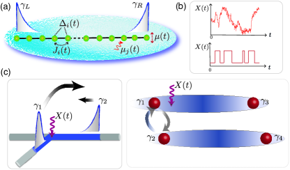
Figure 1: Schematic of Majorana edge modes in noisy Kitaev wires and braiding operations in presence of colored Markovian noise. (a) A Kitaev wire in the topological phase supports two Majorana edge modes $\gamma_{L/R}$. In realistic implementations, a noisy Kitaev Hamiltonian (1) containing stochastic parameters $X(t)\equiv\{J_{j}(t),\Delta_{j}(t),\mu_{j}(t)\}$ arises, due to a coupling to a classical environment (blue background). The fluctuations can be either global [e.g. $\mu(t)$], or local [e.g. $\mu_{j}(t)$], depending on the physical sources of noise in specific implementations. (b) Two typical examples of colored Markovian noise $X(t)$: the colored Gaussian noise (upper panel) and the two-state telegraph noise (lower panel). (c) Braiding Majoranas (say, $\gamma_{1}$ and $\gamma_{2}$) on a noisy T-junction in solid-state setting (left panel), and in a noisy atomic wire network in the optical lattice setup (right panel).

However, while the promise of topological protection of quantum states from microscopic imperfections may hold for static disorder (see e.g. Refs. Nayak2008 ; Pachos2012 ), recent theoretical studies have concluded that Majorana qubits and braiding can be seriously affected by coupling to an environment Goldstein2011 ; Budich2012 ; Raninis2012 ; Pedrocchi2015 ; Hu2014 , as will be the case in any realistic experimental scenario. The protection of Majorana modes in the Kitaev wire is related to protection of fermion parity, and quantum correlations between Majorana states will be rapidly destroyed by injection or removal of quasiparticles Raninis2012 . Even the coupling to a finite temperature bosonic bath, which preserves particle parity, is predicted to result in unavoidable losses of coherence and errors Pedrocchi2015 . Nevertheless, as we will show in this paper, it is possible to identify examples with long-lived quantum correlations between Majorana states in the presence of noise. In particular, we will be interested in the effects of local and global noise representing a parity-preserving coupling to an environment, which we model as a classical stochastic process. The case of local noise is representative of a two-level fluctuator in a solid state realization of a Kitaev wire, while global fluctuations can result, for example, from laser light fluctuations in cold-atom experiments.

Our goal is thus to study the effects of noise on Majorana correlations and braiding operations, in a regime ranging from quasi-static disorder, all the way to the limit of fast fluctuations, i.e. where the noise correlation time is much shorter than the relevant system time scales. Although coupling to classical noise will eventually always lead to dephasing and heating, dephasing can be suppressed in the fast fluctuation limit, even when the system is driven by the noise e.g. between topological and non-topological phases. This effect of noise suppression with decreasing correlation time is familiar from atomic physics as motional narrowing. There, increasing the collision rate between atoms can result in a narrowing of the spectral lines CohenTannoudji1977 , and in our context in an increased coherence time of Majorana correlations. In such cases, we will also determine the optimal conditions for braiding time scales - as a trade off between the requirement of adiabaticity of braiding, and decoherence time scales.

The emphasis and value of the present work is on exactly solvable models quantum many-body dynamics of Majorana correlations and braiding operations in the presence of colored Markovian noise sources, as exemplified by telegraph noise, $n$-state jump models, or colored Gaussian noise. While in a solid state context this should be understood as phenomenological models of noise describing imperfections like local fluctuators, we note that noise in cold atom experiments can be engineered, as in recent studies of Anderson localization with (static) random optical potentials Giacomo2008 ; Billy2008 . Atomic realizations of Majorana fermions may thus serve as an ideal platform to study the effect of time dependent disorder in a controlled setting by appropriate modulation of the laser beams to mimic various noise sources, and can thus provide a direct experimental counterpart to the present theoretical study.

The paper is organized as follows. In Sec. II, we briefly describe the model Hamiltonian of a noisy Kitaev wire. Then, in Sec. III, we develop techniques which allow non-perturbative solutions of the many-body quantum dynamics for colored Markovian noise with arbitrary correlation time. Based on these techniques, Sec. IV presents a study on the Majorana edge correlations and heating dynamics for a global noise, which stochastically drives the system e.g. across the boundary between the topological and non-topological phases. The case of local noise is investigated in Sec. V. Thereafter, in Sec. VI, we study the effect of colored noise on Majorana transport, and discuss optimal conditions for Majorana manipulations to obtain the best fidelity at a given noise. The braiding dynamics on a noisy wire network is analyzed in Sec. VII, based on the noisy T-junction architecture and cold-atom setup, respectively. The paper closes with a summary and outlook in Sec. VIII.

II Noisy Kitaev wire

Our goal is to study the dynamics of Majorana edge modes of the Kitaev wire in the presence of noise (see Fig. 1). The relevant Hamiltonian is

$$H[X(t)] = \sum_{j=1}^{N-1}\left[-J_{j}(t)a_{j}^{{\dagger}}a_{j+1}+\Delta_{j}(t)a_{j}a_{j+1}+\text{h.c.}\right]$$ (1)

$$- \sum_{j=1}^{N}\mu_{j}(t)a_{j}^{{\dagger}}a_{j},$$

where $a_{j}$ and $a_{j}^{{\dagger}}$ are the operator of spinless fermions on a finite chain of $N$ sites. Here $J_{j}(t)$ is the hopping amplitude on the lattice, $\Delta_{j}(t)$ is the pairing parameter and $\mu_{j}(t)$ is the local chemical potential. We assume that these parameters fluctuate in time according to a given noise model $X(t)\equiv\{J_{j}(t),\Delta_{j}(t),\mu_{j}(t)\}$, which is motivated by a particular physical noise source related to a specific implementation. In hybrid nano-wires the above Hamiltonian (or its continuous version) arises from a combination of spin-orbit coupling of electrons in the presence of a magnetic field, and the coupling to an $s$-wave superconductor Sau2010 ; Lutchyn2010 ; Alicea2010 ; Oreg2010 ; Mourik2012 ; Deng2012 ; Rokhinson2012 ; Das2012 ; Churchill2013 ; Finck2013 ; NadjPerge2014 . Thus the effect of a two-level fluctuator, for example, can be represented by a fluctuating local chemical potential $\mu_{j}(t)$ on a given lattice site. On the other hand, a realization of the Kitaev wire with cold fermionic atoms in a 1D optical lattice results from a laser induced coupling to a molecular Bose-Einstein condensate, where a molecule is dissociated into a pair of fermions in the wire, thus realizing the pairing term $\Delta_{j}$ Jiang2011 ; Nascimbene2013 ; Hu2014 . Frequency fluctuations of the laser light can be understood as fluctuations of the laser detuning, or as a global fluctuating chemical potential $\mu_{j}(t)\equiv\mu(t)$.

Before investigating the dynamics of the noisy wire (1), let us briefly describe as a reference the properties of a noise-free Kitaev’s quantum wire Kitaev2001 , where $J_{j}(t)=J$, $\Delta_{j}(t)=\Delta$, and $\mu_{j}(t)=\mu$. When $|\mu|<2J$ and $\Delta\neq 0$, the wire is in the topological phase characterized by a gapped energy spectrum in the bulk and by a pair of robust Majorana edge modes $\gamma_{L}=\gamma_{L}^{{\dagger}}$ and $\gamma_{R}=\gamma_{R}^{{\dagger}}$ of the form $\gamma_{L/R}=\sum_{j}f_{L/R,j}c_{j}$ [here we use the Majorana representation $c_{2j-1}=a_{j}+a_{j}^{{\dagger}}$ and $c_{2j}=-i(a_{j}-a_{j}^{{\dagger}})$ of the operators] with $f_{L/R,j}$ being exponentially localized near the left ($L$) and right ($R$) edges with the localization length $l_{M}$. The pair of Majorana edge modes represents a non-local fermionic zero-energy mode $\alpha_{M}=(\gamma_{L}+i\gamma_{R})/2$, and the long-range correlations $-i\langle\gamma_{L}\gamma_{R}\rangle$ between the Majorana edge states, which are of interest for us, are directly related to the occupation of this mode, $-i\langle\gamma_{L}\gamma_{R}\rangle=1-2\langle\alpha_{M}^{{\dagger}}\alpha_{M}\rangle$. The robustness of the correlations is therefore related to the conservation of fermionic parity which distinguishes the two degenerate ground states with empty and occupied mode $\alpha_{M}$. For $|\mu|>2J$, when the wire is in the non-topological phase, there are no Majorana edge states and all excitations are gapped.

The presence of noisy components in the parameters of the Hamiltonian (1) results in random “shaking” of the system giving rise to changes in population of the $\alpha_{M}$-mode (accompanied by creation of bulk excitations) and, therefore, to the decay of the Majorana correlations. Large-amplitude global noise, say, in the chemical potential, can also drive the system across the quantum phase transition between different phases – topological and non-topological ones, i.e. between the cases with two Majorana edge modes and with none of them. Understanding the fate of Majorana edge modes, the correlations between them, and their braiding in the noisy Kitaev wire (1) involves the study of many-body non-equilibrium dynamics induced by the noise, and we describe the developed techniques for treating such problems in Sec. III.

III Quantum dynamics in colored Markovian noise

In dynamics of quantum systems external noise appears as stochastic parameters in the Hamiltonian, as in Eq. (1), and the time-dependent density matrix equation becomes a multiplicative stochastic differential equation Gardiner2010Stochastic ; VanKampen1976 . Solving for the averaged density matrix in presence of noise with arbitrary correlation times, requires the development of non-perturbative techniques. For fast fluctuations, when the noise correlation time is much shorter than the system response time (white noise limit), a perturbative treatment, in form of a lowest order cumulant expansion, results in a master equation for the stochastically averaged density matrix Gardiner2010Stochastic ; VanKampen1976 . However, with increasing correlation time, the system response will be sensitive to all higher order correlation functions, and in the limit of infinite correlation time the static disorder problem is recovered (as in Anderson Anderson1958 , and many-body localization Huse2010 ). In solving for quantum correlations and braiding dynamics in the noisy Kitaev wire we will rely on Markovian models of colored noise, which allow an exact solution of many-body dynamics for arbitrary correlation time of the noise.

At the heart of our solution of quantum dynamics for colored Markovian noise is the generalized master equation for the marginal system density operator. In brief, we assume a Markov process $X(t)\equiv\{X_{\alpha}(t)\}$, and we denote by $H[X(t)]$ the associated system Hamiltonian. Our goal is to solve the stochastic density matrix equation ($\hbar\equiv 1$), $\partial_{t}\rho(t)=-i\Big{[}H[X(t)],\rho(t)\Big{]}$, with $\rho(t)$ the density operator, for the stochastic average $\langle\rho(t)\rangle_{s}$ with angular brackets denoting the noise average. Defining a marginal density matrix

$$\rho(X,t)=\left\langle\rho(t)\delta(X(t)-X)\right\rangle_{s},$$ (2)

we can derive the generalized master equation for the marginal density matrix (see Ref. Peter1981 and App. A)

$$\partial_{t}\rho\left(X,t\right)=\mathcal{L}\left(X\right)\rho\left(X,t\right)-i\left[H\left(X\right),\rho\left(X,t\right)\right],$$ (3)

with $X$ now a time independent variable. Here $\mathcal{L}(X)$ is generator of our Markovian noise model, as appears in the differential Chapman-Kolmogorov equation for the conditional density $P(X,t|X^{\prime},t^{\prime})$ Gardiner2010Stochastic

$$\partial_{t}P(X,t|X^{\prime},t^{\prime})=\mathcal{L}(X)P(X,t|X^{\prime},t^{\prime}).$$ (4)

Thus the operator $\mathcal{L}(X)$ provides a complete specification of our noise model, and appears as a damping operator in the generalized master equation (3). Solving (3) for $\langle\rho(t)\rangle_{s}=\int dX\rho(X,t)$ provides us with the desired average. We refer to App. B for a discussion of various limits of solving the above equation: this includes the regime of quasi-static disorder, and the fast fluctuation limit (master equation limit). We emphasize, however, that by solving (3) we obtain solutions valid for arbitrary correlation time.

The most general models for classical Markovian noises Gardiner2010Stochastic are described by diffusion processes with continuous noise trajectory and by jump processes with $X(t)$ taking a set of discrete values $\{X_{m}\}$ ($m=0,...,N_{r}$). In the former case, $\mathcal{L}(X)$ corresponds to the Fokker-Planck operator, and a primary example is the colored Gaussian noise (Ornstein-Uhlenbeck process), see upper panel of Fig. 1(b). In the latter $\mathcal{L}(X)$ reduces to a matrix $\mathcal{L}_{mn}$ describing the jump-rates between different $X_{m}$, as in the case of multi-state telegraph noise, see lower panel of Fig. 1(b) for the two-state telegraph noise. While the solution for a diffusion process can in principle be obtained in terms of the eigenfunctions of the Fokker-Planck operator $\mathcal{L}(X)$ Gardiner2010Stochastic ; Peter1981 , we pursue here a much more convenient strategy by discretizing it to a $N_{r}$-state jump model with large $N_{r}$ and properly chosen $\mathcal{L}_{mn}$ – “putting the noise on a lattice”. In this case the generalized master equation (3) takes on the form of a set of coupled equations for marginal density matrices $\rho(X_{m},t)$

$$\!\!\!{\partial_{t}}\rho(X_{m},t)=\sum_{n=0}^{N_{r}}\mathcal{L}_{mn}\rho(X_{n},t)-i[H(X_{m}),\rho(X_{m},t)],$$ (5)

which - at least for low-dimensional processes $X(t)$ - is not significantly of more effort to solve than the original non-stochastic version.

Below we will illustrate above techniques for the Markovian two-state jump model [see lower panel of Fig. 1(b)], which represents the simplest but relevant example capturing all essential features of noise dynamics. It also allows a straightforward extension to multi-state jump models, or to noise from several fluctuators, which for a large number in the sense of the central limit theorem approaches colored Gaussian noise (see App. C). In addition, we will specialize the above equations to the case of a quadratic many-body Hamiltonian, as relevant for the Kitaev wire.

In two-state telegraph noise, the stochastic parameter $X(t)$ switches randomly between two discrete values $a$ and $b$ with rate $\kappa$. Equation (4) is now a rate equation for the probabilities $P(a,t)$ and $P(b,t)$ to be in state $a$ or $b$ respectively,

$$\frac{d}{dt}\Big{[}\begin{array}[]{c}P(a,t)\\ P(b,t)\end{array}\Big{]}=\Big{[}\begin{array}[]{cc}-\kappa&\kappa\\ \kappa&-\kappa\end{array}\Big{]}\Big{[}\begin{array}[]{c}P(a,t)\\ P(b,t)\end{array}\Big{]}:=\mathcal{L}\Big{[}\begin{array}[]{c}P(a,t)\\ P(b,t)\end{array}\Big{]}.$$ (6)

We have $\left\langle X\right\rangle_{s}=(a+b)/2$ and $\left\langle X(t+\tau),X(t)\right\rangle_{s}=\sigma^{2}\exp\left(-|\tau|/\tau_{c}\right)$ for the mean value and first order correlation function, respectively, with $\tau_{c}=1/2\kappa$ the correlation time and the variance $\sigma^{2}={(a-b)^{2}}/{4}$ (using the notation $\left\langle X,Y\right\rangle_{s}\equiv\left\langle XY\right\rangle_{s}-\left\langle X\right\rangle_{s}\left\langle Y\right\rangle_{s}$).

The dynamics of a Kitaev wire driven by a single telegraph noise can be readily derived in the Majorana representation, where the quadratic Hamiltonian (1) can be recast as $H[X(t)]=(1/4)\sum_{il}h_{il}[X(t)]c_{i}c_{l}$, with $h_{il}=-h_{li}$ being an asymmetric Hamiltonian matrix Kitaev2001 . In the Majorana basis, the key quantity capturing the system dynamics is the covariance matrix $\langle{\Gamma(t)}\rangle_{s}=\text{ Tr}[\langle\rho(t)\rangle_{s}\hat{\Gamma}]$, with $\hat{\Gamma}_{il}=(i/2)[c_{i},c_{l}]$. Thus from Eq. (5), we find for the marginal densities

$$\frac{d}{dt}{\Gamma}(a,t) = -i[h(a),{\Gamma}(a,t)]-\kappa{\Gamma}(a,t)+\kappa{\Gamma}(b,t),$$

$$\frac{d}{dt}{\Gamma}(b,t) = -i[h(b),{\Gamma}(b,t)]-\kappa{\Gamma}(b,t)+\kappa{\Gamma}(a,t).$$ (7)

The desired stochastic average is $\langle\Gamma(t)\rangle_{s}={\Gamma}(a,t)+{\Gamma}(b,t)$. Before proceeding with the general solution, we find it worthwhile to briefly comment on the fast and slow (quasi-static disorder) limit.

In the fast noise limit, when $1/\kappa$ is the shortest time scale, an adiabatic elimination of the fast dynamics in lowest order perturbation theory reduces the above equations to a master equation in Lindblad form,

$$\frac{d}{dt}{\langle\Gamma\rangle}_{s}=-i\left[h_{+},\langle\Gamma\rangle_{s}\right]-\frac{1}{2\kappa}\left[h_{-},\left[h_{-},\langle\Gamma\rangle_{s}\right]\right],$$ (8)

with $h_{\pm}=[h(a)\pm h(b)]/2$. The first term describes a coherent evolution with the average Hamiltonian $h_{+}\equiv\langle h\rangle_{s}$, while the second term is the noise-induced damping, which scales as $1/\kappa$. Suppression of the dissipation by fast noises is called motional narrowing in an atomic physics context CohenTannoudji1977 , and corresponds to a Zeno effect Facchi2008 . If the average Hamiltonian is in the topological phase and thus supports Majorana edge modes, the initial Majorana correlation will show slow dephasing due to the Zeno effect - irrelevant if $a$ or $b$ per se lies in the topological or non-topological regime. On the other hand, in the limit of slow noise, i.e. when the jump rate $\kappa\rightarrow 0$, we can ignore $\mathcal{L}$ in Eqs. (3) and (7), $\mathcal{L}\rightarrow 0$, during long times $t\ll\kappa^{-1}$, so that for such times we simply have to perform the (quasi-)static average of the system dynamics.

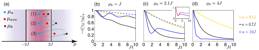
Figure 2: Evolution of Majorana edge correlations in presence of globally fluctuating chemical potential. (a) For a chemical potential $\mu(t)$ flipping between $\mu_{a}$ and $\mu_{b}$, there exist three jump scenarios (1)-(3) in the phase diagram corresponding to the value of $\mu_{b}$. (b)-(d) Time evolution of the Majorana edge correlation function $-i\langle\gamma_{L}\gamma_{R}\rangle_{s}$ for $\mu_{a}=0.2J$ and (b) $\mu_{b}=J$ (c) $\mu_{b}=2.1J$ and (d) $\mu_{b}=4J$. In each scenario, we take three typical jump rates: $\kappa=0.1J$, $\kappa=0.7J$, and $\kappa=10J$, and consider a Kitaev wire of $N=60$ sites with the pairing parameter $\Delta=0.8J$. We have considered two types of initial conditions, which correspond to the ground state of Hamiltonian $H_{a}$ (solid curves) and of average Hamiltonian $H_{\text{ave}}$ in the case of fast noises [blue dashed curves in (b) and (c)]. In the inset of (c), the dynamics for the noise with $\kappa=10J$ (blue curve) for $\mu_{b}=2.1J$ is compared with the quench dynamics (red curve), for a quench in the chemical potential from $\mu=0.2J$ to $\mu=\mu_{\textrm{ave}}$.

Below we will solve the full marginal density equations (7) for Majorana edge correlation $-i\langle\gamma_{L}\gamma_{R}\rangle_{s}=-\sum_{il}f_{L,i}f_{R,l}\langle\hat{\Gamma}_{il}\rangle_{s}$, with $f_{L/R,l}$ the Majorana wavefunction of the initial Hamiltonian in the Majorana basis. Our discussion will focus on the special case of local and global telegraph fluctuations of the chemical potential. As mentioned above, such telegraph noise can represent a local two-level fluctuator in a solid state setup, and global laser frequency noise in an atomic realization of the Kitaev wires. We would like to stress, however, that even though we consider here the simplest jump-like noise process and only the chemical potential as a fluctuating parameter, our conclusions remain valid for a more general scenario with colored noise and with several fluctuating parameters.

We conclude this section with the remark that the considered Markovian noise models give rise to first order noise correlation functions, which are exponentials, or superposition of exponentials. We note however that non-Markovian noise models can often be represented as projections of higher dimensional Markov processes, which can also be solved by our techniques. Another point to mention is that for non-quadratic Hamiltonians in one dimension, the generalized master equation (3) can be solved using the density matrix renormalization method Daley2004 ; Schollwock2005 , and the developed techniques therefore are interesting in a much broader context for many-body systems driven by colored noise.

IV Edge and bulk dynamics in presence of global noise

We begin with discussing the time evolution of the Majorana edge correlation $-i\langle\gamma_{L}\gamma_{R}\rangle_{s}$ under the global fluctuations in the chemical potential $\mu(t)$, when it flips between two values $\mu_{a}$ and $\mu_{b}$ (the corresponding Hamiltonian are $H_{a}$ and $H_{b}$, respectively) with the jump rate $\kappa$. The statistic property of $\mu(t)$ is described by the mean value $\mu_{\text{ave}}=(\mu_{a}+\mu_{b})/2$, the variance $\sigma^{2}=(\mu_{a}-\mu_{b})^{2}/4$, and the correlation time $\tau_{c}=1/2\kappa$. We denote by $H_{\text{ave}}=\langle H[\mu(t)]\rangle_{s}$ the average Hamiltonian over the noise realization, which in the considered case is of the form of a noise-free Kitaev Hamiltonian with $\mu=\mu_{\text{ave}}$. For the initial condition, we take $\mu(0)=\mu_{a}$ with $|\mu_{a}|<2J$ such that Hamiltonian $H_{a}$ is in the topological phase, and assume the system is in the ground state with the Majorana edge-mode correlation $-i\langle\gamma_{L}\gamma_{R}\rangle=1$. For the value $\mu_{b}$, we consider three possible scenarios (see Fig. 2(a)): (1) $|\mu_{b}|<2J$, when the Hamiltonian $H_{b}$ is in the topological phase (fluctuations within the topological phase); (2) $|\mu_{b}|>2J$ but $|\mu_{\text{ave}}|<2J$, when $H_{b}$ is in the non-topological phase but the average Hamiltonian $H_{\text{ave}}$ remains in the topological phase (fluctuations between topological and non-topological phases but on average staying in the topological one); and (3) $|\mu_{b}|>2J$ and $|\mu_{\text{ave}}|>2J$, when both Hamiltonians $H_{b}$ and $H_{\text{ave}}$ are non-topological (large-amplitude fluctuation when staying on average in the non-topological phase). The evolution of $-i\langle\gamma_{L}\gamma_{R}\rangle_{s}$ calculated on the basis of Eq. (7) for these three scenarios, is shown in Figs. 2(b) - 2(d), respectively, in the regimes of fast, intermediate, and slow jump rate $\kappa$.

We see that noise always leads to decay of Majorana correlations, but the decay dynamics significantly depends on the amplitude and rate of the noise. Non-surprisingly, we find the slowest decay of the Majorana correlations in the scenario (1) when the fluctuating Hamiltonian always remains in the topological phase. Strikingly, the dynamics in the scenario (2) shows the same features, even though here we have jumps between topological and non-topological phases: In both scenarios, we observe the fastest decay in the regime with an intermediate jump rate ($\kappa=0.7J$, black curves in Figs. 2(b) and 2(c)), when $\kappa$ is comparable with the energy gap and the band width ($\sim J\sim\Delta$) of the Hamiltonian $H_{a}$; whereas, in both slow ($\kappa=0.1J$, yellow curves) and the fast noise ($\kappa=10J$, blue curves) regimes, the decay is much slower, and the system exhibits substantial Majorana correlations for much larger times ($>10J^{-1}$). In contrast to this non-monotonic dependence on the noise rate, the decay rate in the scenario (3) grows with $\kappa$ (see Fig. 2(d)): for both intermediate and fast fluctuations there are no visible Majorana correlations for times $t\gtrsim 10J^{-1}$, although for slow noise they survive for a much longer time.

We now detail the analysis on the dynamical behavior of $-i\langle\gamma_{L}\gamma_{R}\rangle_{s}$ in scenarios (1)-(3) in the slow, fast and intermediate regimes of the noise, respectively. We start with slow fluctuations when $\kappa\ll J\sim\Delta$, $\mu_{a(b)}$. In this case, the quenches between $H_{a}$ and $H_{b}$ – occuring at random instants – on average take place after a typical time $\kappa^{-1}$, which is much larger than all characteristic time scales of the system. As is explained in App. D, on the time scale of several inverse band-widths of the system ($\sim J^{-1}$) after a quench, the Majorana correlations relax to asymptotic values which are determined by the overlap of the Majorana edge-mode wave-functions for the Hamiltonians $H_{a}$ and $H_{b}$. Such asymptotic values then remain constant till the next quench occurs. For the scenarios (2) and (3), when $H_{b}$ is non-topological and has no edge modes, the overlap is zero, and already the first quench completely destroys the correlations. We therefore have $-i\langle\gamma_{L}\gamma_{R}\rangle_{s}\sim\exp(-\kappa t)$ for these scenarios (yellow curves in Figs. 2(c) and 2(d)). On the other hand, for the scenario (1) when $H_{b}$ has the zero mode, the overlap is non-zero. In this case, each quench reduces the correlations by a factor of $G_{\infty}<1$ related to the overlap [see Eqs. (23) and (25) in App. D], resulting in a slower decay of the correlation $-i\langle\gamma_{L}\gamma_{R}\rangle_{s}\sim\exp[-\kappa(1-G_{\infty})t]$ (yellow curve in Fig. 2(b)).

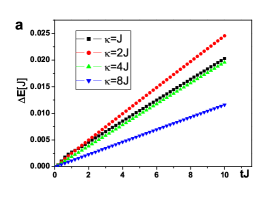
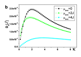
Figure 3: Heating dynamics in the bulk. (a) The absorbed energy $\Delta E(t)$ in unit of $J$ as a function of time for $\mu_{\text{ave}}=0$ and different $\kappa$; (b) Heating rate $D_{s}$ in unit of $J^{2}$ as a function of $\kappa$ for different $\mu_{\text{ave}}$. Numerical results (dotted curves) are compared to the predictions from Eq. (11) (solid curves). For (a)-(b), we have fixed the noise variance $\sigma=|\mu_{b}-\mu_{a}|/2=0.1J$, and have chosen $\Delta=J$.

In the opposite regime of fast fluctuations ($\kappa\gg|\mu_{b}-\mu_{a}|$, $J\sim\Delta$), the dynamic behavior is remarkably related to the Zeno effect and to the quench problem. In this case, the evolution of $-i\langle\gamma_{L}\gamma_{R}\rangle_{s}$ can be explained based on Eq. (8) for the correlation matrix, which in the considered case takes the form

$$\frac{d}{dt}\langle\Gamma\rangle_{s}=-i[h_{+},\langle\Gamma\rangle_{s}]-\frac{\sigma^{2}}{2\kappa}[{N},[{N},\langle\Gamma\rangle_{s}]].$$ (9)

Here $\sigma=|\mu_{b}-\mu_{a}|/2$ as mentioned earlier, and the matrices $h_{+}$ and $N$ correspond to the Hamiltonian $H_{\text{ave}}$ and the total particle number operator in the Majorana basis. Following from Eq. (9), we see that:

(i) In the limit $\kappa\rightarrow\infty$, when the second ‘decay’-term can be neglected, Eq. (9) describes the dynamics of correlations after the quench from the initial Hamiltonian $H_{a}$ to the averaged one $H_{\text{ave}}$. As a result, the asymptotic ($t\rightarrow\infty$) value of the Majorana correlation function $-i\langle\gamma_{L}\gamma_{R}\rangle_{s}$ is determined again by the overlap of the wave functions of the Majorana edge modes (see App. D), but now for the Hamiltonians $H_{a}$ and $H_{\text{ave}}$. For Hamiltonian $H_{\text{ave}}$ in the non-topological phase [scenario (3)], there are no such modes, and after the quench $-i\langle\gamma_{L}\gamma_{R}\rangle_{s}$ decays to zero on the time scale of the order of the inverse band-width of $H_{\text{ave}}$. For $H_{\text{ave}}$ in the topological phase, [scenario (1) with topological $H_{b}$ and scenario (2) with non-topological $H_{b}$], this mode exists giving rise to a non-zero overlap and to a finite asymptotic value of the correlations after the quench.

(ii) For a large but finite $\kappa$, the second term in Eq. (9) adds a slow decay on top of the quench dynamics, providing the asymptotic behavior of $-i\langle\gamma_{L}\gamma_{R}\rangle_{s}$ shown in Figs. 2(b) and 2(c). The short-time ($t\lesssim J^{-1}$) behavior of the correlations, seen in the form of damped oscillations on these figures, is sensitive to the details of the band structures of $H_{a}$ and $H_{\text{ave}}$. In general, the ‘closer’ these Hamiltonians are, the more pronounced are the oscillations, and the less destructive effect has the quench on $-i\langle\gamma_{L}\gamma_{R}\rangle_{s}$.

(iii) Note that Eq. (9) suggests the preparation of the initial Majorana correlations with respect to the edge states of the Hamiltonian $H_{\text{ave}}$, not $H_{a}$, which is practically also more natural for fast fluctuations. In this case, the first term in Eq. (9) has no destructive effects, and $-i\langle\gamma_{L}\gamma_{R}\rangle_{s}$ shows slow decay due to the second term (dashed blue lines in Figs. 2(b) and 2(c)). This slow decay of Majorana correlations in presence of fast noises – even for a sufficiently large fluctuation amplitude outside the topological phase – is a direct consequence of the Zeno effect, which reduces the dynamics with fast fluctuating parameters to a weakly damped dynamics with the averaged Hamiltonian.

Finally, in the intermediate regime when the fluctuation rate is of the order of typical energy scales in the system, $\kappa\sim J\sim\Delta$, $\mu_{a(b)}$, one has optimal conditions for pumping excitations into the system (heating), leading to the fastest decay of the Majorana correlations. This can be seen by looking at the growth in the system energy under the action of noises. To illustrate this heating dynamics, we consider the case when $\mu(t)$ jumps between $\mu_{a}=\mu-\delta\mu$ and $\mu_{b}=\mu+\delta\mu$ (such that $\mu_{\mathrm{ave}}=\mu$) with a rate $\kappa$, focusing on the weak noise limit $\delta\mu\ll J$ and choosing $\Delta=J$. We assume that initially the system is in the ground state of the average Hamiltonian $H_{\text{ave}}$ [but still $\mu(t=0)=\mu_{a}$], with energy $E_{0}$ calculated with the corresponding initial density matrix $\rho_{s}(0)$, and calculate the system energy gain $\Delta E(t)=\text{Tr}(\rho_{s}(t)H_{\mathrm{ave}})-E_{0}$ for different $\mu$ and $\kappa$. A typical time evolution of $\Delta E(t)$ for different noise jump rates is shown in Fig. 3(a). There, the energy is seen to grow linearly, $\Delta E(t)=D_{s}t$, after a short transition time ($t\lesssim J^{-1}$). Then after a relatively long time (not shown) due to the small noise amplitude $\delta\mu\ll J$, it saturates to the asymptotic value which depends on $\mu$ but not on $\kappa$ (infinite-temperature state). The heating rate $D_{s}$ depends on both $\kappa$ and $\mu$. Figure 3(b) shows $D_{s}$ as a function of the jump rate $\kappa$ for the values of chemical potential $\mu=0$, $2J$, and $4J$, which correspond to the topological, critical, and non-topological phases, respectively. We see that $D_{s}$ is a non-monotonic function of $\kappa$, which is small when noise is slow or fast (Zeno effect), and has a pronounced maximum for $\kappa\approx 2-4J$. The maximum corresponds to the situation when the inverse noise correlation time $\tau_{c}^{-1}=2\kappa$, which determines the frequency width of the noise correlation function, lies inside the band of bulk excitations (the exact position depends on the band structure).

The linear growth of the energy for the considered times can be understood by calculating the energy gain in the second-order perturbation theory ($\hbar\equiv 1$):

$$\Delta E(t)=\sum_{\nu}\varepsilon_{v}\left|M_{\nu}\right|^{2}\left\langle\left|\int_{0}^{t}d\tau\exp(i\varepsilon_{\nu}\tau)\mu(\tau)\right|^{2}\right\rangle,$$ (10)

where $M_{\nu}$ is the matrix element of the number operator between the ground state and the excited state $\left|\nu\right\rangle$ with the energy $E_{0}+\varepsilon_{\nu}$. For the considered global perturbation, $\left|\nu\right\rangle$ simply corresponds to the state with two single-particle excitations with momenta $k$ and $-k$, and the energy $\varepsilon_{\nu}=2E_{p}=2\sqrt{(2J\cos pa+\mu)^{2}+4\Delta^{2}\sin^{2}pa}$ with $a$ being the lattice spacing. Performing the time derivative and assuming the time $t$ being larger than the noise correlation time $\tau_{c}=(2\kappa)^{-1}$, we obtain the following expression for $D_{s}$:

$$D_{s}=\sum_{p}2E_{p}\left|M_{p}\right|^{2}\int_{-\infty}^{\infty}d\tau\left\langle\mu(\tau)\mu(0)\right\rangle\exp(2iE_{p}\tau),$$

where the summation is over the Brillouin zone $p\in(-\pi/a,\pi/a]$. With the expression $\left|M_{p}\right|^{2}=\left|u_{p}v_{p}\right|^{2}=(\Delta^{2}\sin^{2}pa)/E_{p}^{2}$ for the matrix element and $\left\langle\mu(\tau)\mu(0)\right\rangle=\mu^{2}+\sigma^{2}\exp(-2\kappa\left|\tau\right|)$ for the noise correlation function, we finally obtain ($k=pa$)

$$D_{s}=4\sigma^{2}\int_{-\pi}^{\pi}\frac{dk}{2\pi}\frac{\kappa}{\kappa^{2}+E^{2}_{k}}\frac{\Delta^{2}\sin^{2}k}{E_{k}},$$ (11)

for the energy-growth coefficient. The above expression is plotted as solid lines in Fig. 3(b) and is in very good agreement with numerical data.

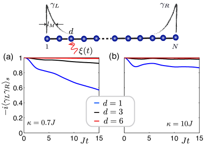
Figure 4: The effect of local noise at different locations in a Kitaev wire on Majorana edge correlations. (a)-(b) Time evolution of $-i\langle\gamma_{L}\gamma_{R}\rangle_{s}$ when a noise $\xi(t)$ arises in the local chemical potential at three different sites ($d=1,3,6$), with a jump rate (a) $\kappa=0.7J$ and (b) $\kappa=10J$. We take $\xi_{a}=0$ and $\xi_{b}=0.8J$, $N=60$, $\Delta=0.4J$, and $\mu=0.4J$. For this parameter choice, the localization length of the Majorana modes is $l_{M}\approx 2.5a$, with $a$ being the lattice constant.

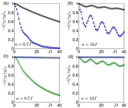
Figure 5: (a)-(b) The effect of a large-amplitude noise $\xi(t)$ in the local chemical potential on the dynamics of Majorana edge correlation $-i\langle\gamma_{L}\gamma_{R}\rangle_{s}$, when the local noise $\xi(t)$ arises at site $d=3$ (blue curves) and $d=6$ (black curves), flipping between $\xi_{a}=0$ and $\xi_{b}=4.4J$. (c)-(d) Evolution of the edge correlation $-i\langle\gamma_{L}\gamma_{R}\rangle_{s}$ when noise induces at random instants a splitting in the wire, between sites $3$ and $4$ (green curves) and between sites $6$ and $7$ (blue curves). In (a)-(d), we take two different noise jump rates, $\kappa=0.7J$ (left panels) and $\kappa=10J$ (right panels). Other parameters are the same as Fig. 4.

V Local noise

We next discuss the effects of the local noise on the Majorana correlations $-i\langle\gamma_{L}\gamma_{R}\rangle_{s}$, which we model by adding a fluctuating part to the chemical potential on the site $d$, such that $\mu_{j}(t)=\mu+\delta_{j,d}\xi(t)$ with the amplitude $\xi(t)$ being described by the telegraph noise: $\xi(t)$ randomly flips between $\xi_{a}$ and $\xi_{b}>0$ with the rate $\kappa$, and $\xi(0)=\xi_{a}$. In this case, an exponential localization of the Majorana modes near the edges with the localization length $l_{M}$ leads to a very strong dependence of the effects of the noise on $d$. This is because the decay of the Majorana correlations is caused by noise-induced changes in the population of the associated non-local fermionic zero-energy mode, with the corresponding matrix element being proportional to the value of the edge-mode wave function on the noisy site $d$. The results of our calculations for intermediate and fast noises, Figs. 4(a) and 4 (b), respectively, clearly show this dependence: the decay is the fastest for $d<l_{M}$, for $d\sim l_{M}$ it is already substantially less, and is exponentially small for $d>l_{M}$.

Similar to the case of a global noise, the reduction of the decay in the fast-noise regime ($\kappa\gg J$, $\Delta$, $\mu$) is due to the Zeno effect, as follows from Eq. (8) which now takes the form

$$\frac{d}{dt}\langle\Gamma\rangle_{s}=-i[h_{+},\langle\Gamma\rangle_{s}]-\frac{\sigma^{2}}{2\kappa}[n_{d},[n_{d},\langle\Gamma\rangle_{s}]],$$

where $\sigma=|\xi_{b}-\xi_{a}|/2$, the matrix $n_{d}$ corresponds to the local density operator $a_{d}^{\dagger}a_{d}$ at site $d$ in the Majorana basis, and the second term adds a slow decay on top of the result of the quench described by the first term. The average Hamiltonian in this case contains the static impurity potential $V_{d}=(\xi_{a}+\xi_{b})/2$ on the site $d$, which results in just modification of the Majorana edge modes, and hence in a finite asymptotic value of $-i\langle\gamma_{L}\gamma_{R}\rangle_{s}$ after the quench. The small ($\sim\kappa^{-1}$) decay rate is extra reduced, as compared to the global noise, for $d\gtrsim l_{M}$ due to the smallness of the edge-mode wave functions on the site $d$. For $d>l_{M}$, this gives an exponentially small decay rate such that the Majorana correlations are practically immune to the noise (Fig. 4).

If we increase the amplitude of the noise to larger values, see Figs. 5(a) and 5(b) for $\xi_{b}=4.4J$, the oscillating behavior for fast noise become much more pronounced. In this case, the strong static impurity potential in the average Hamiltonian splits the wire into two pieces which are weakly coupled through the impurity site (Josephson junction). If the coupling would be zero, one would have an extra pair of Majorana modes at the edges adjacent to the impurity, and the corresponding fermionic zero-mode. For a small but finite coupling, the energy of this mode is finite, and the oscillations seen in this case correspond to the energy of this mode. Similar oscillatory behavior is observed when the fast noise randomly splits the wire into two parts, for example, when the local hopping $J_{d}$ and the pairing $\Delta_{d}$ amplitudes (between site $d$ and $d+1$) jump simultaneously between the finite values and zero, as shown in Figs. 5(c) and 5(d). In this case of fast noise, the average Hamiltonian has a “weak link”, and the oscillation frequency seen in Fig. 5(d) corresponds to the energy of the fermionic mode localized at this link. Note that the amplitude of the oscillations is related to the overlap between the Majorana edge mode and the wave function of the low-energy fermionic mode localized on the “defected” site or link, and rapidly decreases with increasing distance between the modes.

Note that for the ideal Kitaev chain ($J=\Delta$ and $\mu=0$), the two Majorana modes $\gamma_{L}=c_{1}$ ($\gamma_{R}=c_{2N}$) locate on the leftmost (rightmost) sites, such that $-i\langle\gamma_{L}\gamma_{R}\rangle_{s}=-(\Gamma_{s})_{1,2N}$. In this case, the dynamics of the Majorana correlations is completely uncoupled from that of the bulk – the Majorana correlations in this ideal case are absolutely insensitive to what happens in the bulk.

VI Competition between noise and adiabaticity in Majorana Transport

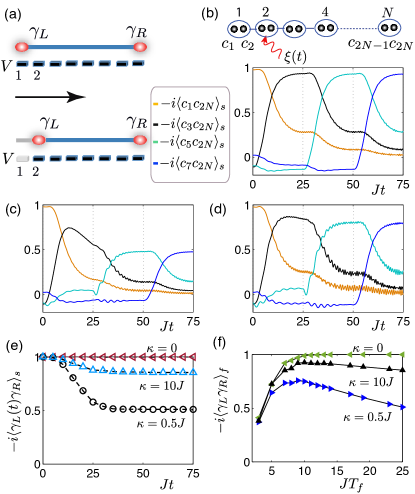
Figure 6: Fate of a Majorana moving through a local noise. (a) A move of the Majorana edge mode $\gamma_{L}$ from site $1$ to site $2$ by adiabatically tuning the local potential $V$ in a time interval $T_{f}$. (b)-(e) Time evolution of the correlation between the edge Majorana operators $-i\langle c_{2j-1}c_{2N}\rangle_{s}$ for $j=1,2,3,4$, when $\gamma_{L}$ is adiabatically transported from site $1$ to site $4$ through a local noise $\xi(t)$ at site $d=2$ with (b) $\kappa=0$ (c) $\kappa=0.5J$ and (d) $\kappa=10J$. (e) The time evolution of the correlations between the Majorana edge modes $-i\langle\gamma_{L}(t)\gamma_{R}\rangle_{s}$ for different $\kappa$. ($JT_{f}=25$ for (b)-(e)). (f) The remaining Majorana correlations $-i\langle\gamma_{L}\gamma_{R}\rangle_{f}$ as a function of $T_{f}$ for different $\kappa$, after $\gamma_{L}$ is moved to site $4$ (in total times of $3T_{f}$). For (b)-(f), we have chosen $\xi_{a}=0$, $\xi_{b}=0.8J$, $N=40$, $\Delta=0.8J$, and $\mu=0.2J$.

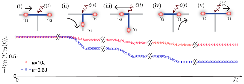
Figure 7: Majorana braiding on a noisy T-junction, where a local noise $\xi(t)$ occurs in the common joint connecting three wire segments. Upper panel: schematics of an exchange of two Majoranas $\gamma_{1}$ and $\gamma_{2}$ following Ref. Alicea2011 : (i) Initially the horizontal wire is topological supporting two Majorana edge modes $\gamma_{1}$ and $\gamma_{2}$ at the ends, while the vertical wire is non-topological. (ii) $\gamma_{1}$ is moved through the junction to the bottom of the vertical wire, while $\gamma_{2}$ is fixed at the right end of the horizontal wire. (iii) $\gamma_{2}$ is moved all the way to the left end of the horizontal wire, while $\gamma_{1}$ is fixed. (iv) $\gamma_{1}$ is moved upward through the junction and then rightward. (v) At the end of the exchange, the wire returns to its original configuration, with $\gamma_{1}\rightarrow\gamma_{2}$ and $\gamma_{2}\rightarrow-\gamma_{1}$. Lower panel: Evolution of the Majorana edge correlations $-i\langle\gamma_{1}(t)\gamma_{2}(t)\rangle_{s}$ in each step of the exchange processes, when a local noise $\xi(t)$ in the junction jumps between $0$ and $0.7J$ at a jump rate $\kappa=0.6J$ and $\kappa=10J$, respectively. For other parameters, the pairing parameter of the horizontal and vertical wires are chosen as $\Delta_{x}=i\Delta_{y}=0.7J$. We take $\mu=0.1J$ in the topological segment and $\mu=-4J$ in the nontopological segment of the wires, and $JT_{f}=18$.

Equipped with above understanding of the non-equilibrium dynamics of a noisy Kitaev wire, we now discuss the effect of a local noise on the Majorana edge correlations during the adiabatic transport Alicea2011 ; Halperin2012 ; Romito2012 – an essential building block for the braiding operations. As we will see, in the presence of a noise, the adiabaticity of the transport – required for preserving the information encoded in the Majorana correlations – confronts with the finite life-time of the correlations, and the competition of these two factors establishes an optimal operation time.

Following Ref. Alicea2011 , we will move the left Majorana edge mode by “pushing” it to the right via adiabatically switching on local potentials on the corresponding sites. For example (see Fig. 6(a)), the move of $\gamma_{L}$ from site $1$ to site $2$ can be achieved by applying the local potential $\lambda(t)V$ at site $1$ [an extra term $\lambda(t)Va_{1}^{{\dagger}}a_{1}$ in the Hamiltonian], where $V\gg 2J$ and $\lambda(t)$ increases monotonically from $\lambda(t<0)=0$ to $\lambda(t>T_{f})=1$ during the time interval $[0,T_{f}]$ with $T_{f}$ being much larger than the inverse energy gap, $T_{f}\gg J^{-1}$, $\Delta^{-1}$, $\mu^{-1}$. (In our calculations we use $\lambda(t)=\sin^{2}[(\pi/2T_{f})t]$.) Further moves can be achieved by applying the same protocol successively to sites $2$, $3$, …. In Fig. 6(b) we show the evolution of the correlations $-i\langle c_{2j-1}c_{2N}\rangle$ with $j=1,2,3,4$, during the adiabatic move of $\gamma_{L}$ from site $1$ to site $4$ for $T_{f}=25J^{-1}$ (in total time $3T_{f}$) and in the absence of the noise. (The correlation $-i\langle\gamma_{L}(t)\gamma_{R}\rangle$ between the actual edge modes remains unchanged from its initial value $1$, see also the curve with $\kappa=0$ in Fig. 6(e)).

The same correlations in the presence of the local noise $V_{d}[\xi(t)]=\xi(t)n_{d}$ at site $d$ [here $\xi(t)$ flips again between $\xi_{a}$ and $\xi_{b}$ at a rate $\kappa$] are shown in Figs. 6(c) ($\kappa=0.5J$) and 6(d) ($\kappa=10J$) for $d=2$. The corresponding behavior of the correlation $-i\langle\gamma_{L}(t)\gamma_{R}\rangle_{s}$ between the edge modes [$\gamma_{L}(t)$ is moving and $\gamma_{R}$ is fixed] is presented in Fig. 6(e). We clearly see deviations from the noise-free case, which are significant for $\kappa=0.5J$ and small for $\kappa=10J$ (Zeno effect), but these deviations take place mostly when the Majorana mode moves to the noisy site (for $t$ from $0$ till $T_{f}$ in the considered example). After that, the Majorana correlations do not exhibit any visible decay and repeat the pattern of the noise-free case but with the reduced amplitudes. This behavior follows from the localized character of wave functions of the Majorana edge states: the correlations between them are influenced by the local noise only when the moving Majorana mode and the noisy site are within the localization length $l_{M}$. (Note that the extend of the edge-mode wave function in the ‘non-topological’ part of the wire – the sites with non-zero local potential $V$– is also non-zero but very small for $V\gg 2J$. As a result, a noisy site in this part of the wire has no effect of the correlations.)

Above results also imply that, in order to minimize the destructive effect of the noise on Majorana edge correlations, the move through the noisy site has to be performed with the fastest speed – the requirement which is opposite to the adiabaticity condition for the transport. As a result, there exists an optimum speed of transport (optimum $T_{f}$) for each $\kappa$. This is illustrated in Fig. 6(f) which shows the remaining correlations (after the total move) as a function of $T_{f}$ for different $\kappa$: the decrease in the correlations for small $T_{f}$ is due to non-adiabatic effects, while for large $T_{f}$ it is due to accumulated action of the noise. The proper choice of $T_{f}$ can substantially reduces the loss of correlations, especially in the intermediate-noise regime.

Similar consideration is also applicable to the global noise. However, in this case the destructive effect of the noise is independent of the position of the Majorana modes, so that an entire time of the operation should be within the life-time of correlations, see Fig. 2.

VII Fidelity of braiding in a noisy wire network

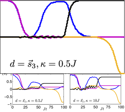
Figure 8: Braiding dynamics of Majoranas in a noisy atomic wire network. (a) Cold-atom implementation of braiding based on Refs. Kraus2013 ; Laflamme2014 , where the Majorana modes $\gamma_{L}^{(u)}$ and $\gamma_{L}^{(l)}$ on the left ends of the two wires are exchanged. (b)-(e) Time evolution of the Majorana correlation functions for (b) noise-free case (c) a local noise at site $\vec{s}_{3}$ of the upper wire with $\kappa=0.5J$, and (d)-(e) a local noise at site $\vec{s}_{1}$ of the upper wire with (d) $\kappa=0.5J$ and (e) $\kappa=10J$. For (c)-(e), we choose $\xi_{a}=0$ and $\xi_{b}=0.6J$. For other parameters, $\Delta^{(u)}=\Delta^{(l)}=0.7J$ and $\mu^{(u)}=\mu^{(l)}=0$, $N^{(u)}=N^{(l)}=32$. Following Refs. Kraus2013 ; Laflamme2014 , the braiding is realized in four steps, where we choose the operation time $t_{f}$ for each step as $Jt_{f}=25$ for (b)-(e)).

Finally, we study the effects of the noise on the Majorana braiding (exchange) – the operation which for the two modes $\gamma_{1}$ and $\gamma_{2}$ corresponds (up to a phase) to the unitary operator $U=\exp{[-(\pi/4)\gamma_{1}\gamma_{2}]}$ and results in the transformation $\gamma_{1}\rightarrow\gamma_{2}$, $\gamma_{2}\rightarrow-\gamma_{1}$, showing non-Abelian character of Majorana fermions Alicea2011 ; Ivanov2001 . We consider two proposed braiding scenarios: (i) in the T-junction for the solid-state heterostructures, see Ref. Alicea2011 , and (ii) in the wire-networks for cold-atom systems, see Refs. Kraus2013 ; Laflamme2014 .

We first consider the T-junction with two Majorana edge modes $\gamma_{1}=\gamma_{L}$ and $\gamma_{2}=\gamma_{R}$ which we braid by moving them, see Fig. 7, in accordance with the protocol from Ref. Alicea2011 . We choose initially $-i\langle\gamma_{1}\gamma_{2}\rangle=1$ and follow the evolution of this correlation during the protocol. Without noise, it remains unchanged during the entire braiding, provided we move the modes, say $\gamma_{1}$, adiabatically (we choose $T_{f}=18J^{-1}$). In the presence of local noise, from the previous results we expect the decrease of $-i\langle\gamma_{1}(t)\gamma_{2}(t)\rangle_{s}$ each time when the Majorana mode passes the noise site. This is demonstrated in Fig. 7 for the case when the noise-source is located at the common point of the three legs forming the T-junction: here the Majorana modes have to cross the noisy site three times, and each crossing results in the decrease of $-i\langle\gamma_{1}(t)\gamma_{2}(t)\rangle_{s}$. For the noisy site located in one of the legs, only two crossings occur with the two corresponding drops in $-i\langle\gamma_{1}(t)\gamma_{2}(t)\rangle_{s}$, resulting in a higher fidelity of the braiding operation.

For the braiding in an atomic wire network, we consider two wires (see Fig. 8(a)): the upper one (u) and the lower one (l), each having a pair of Majorana modes ($\gamma_{L}^{(u)},\gamma_{R}^{(u)}$) and ($\gamma_{L}^{(l)},\gamma_{R}^{(l)}$). The braiding protocol from Refs. Kraus2013 ; Laflamme2014 involves operations only on one side (say, left) of the network, and the mode to be braided, $\gamma_{1}=\gamma_{L}^{(l)}$ and $\gamma_{2}=\gamma_{L}^{(u)}$, are also located on the same side. As a result, the protocol will be only sensitive to noise located close to the left side of the network. Fig. 8(b) shows the evolution of correlations between various Majorana modes during braiding in the absence of the noise. The evolution of the same correlations with the telegraphic-noise source with $\kappa=0.5J$ on the third site ($\vec{s}_{3}$) and on the first site ($\vec{s}_{1}$) of the upper wire are presented in Figs. 8(c) and 8 (d), respectively. They clearly show the above mentioned feature of the protocol. Notably, for a fast noise, even when the noise source is located on the first site $\vec{s}_{1}$, one has much less noise-induced decoherence whence higher fidelity, see Fig. 8(e).

VIII Conclusions and Outlook

To summarize, we have studied the decoherence of Majorana edge correlations and braiding dynamics in colored Markovian noises preserving parity symmetry. Our analysis relies on a technique for solving quantum many-body dynamics when the system parameters undergo local or global fluctuations modelled by classical stochastic processes with arbitrary correlation time. Our studies on noisy Kitaev wires show that, while the noise always gives rise to the decay of the correlations between Majorana edge-states, there are several parameter regimes where the life-time of the correlations remains sufficient for quantum manipulations with Majorana fermions, even without error-corrections. This includes the cases of slow global noise and generic local noise in the bulk, and in particular, the case of fast noise where decoherence can be suppressed due to motional narrowing, also known as the Zeno effect. These results further allow us to optimize the manipulation protocols of Majoranas in both the solid-state and cold-atom settings. Our presentation is for two-level telegraph noises in chemical potentials, but the essential features of noise dynamics are also seen in the colored Gaussian noises (the lattice model), and in other types of noises, e.g. the phase fluctuation in the pairing parameters.

The present study and the development of techniques to treat the effect of noise from static disorder to the rapid fluctuation limit, should also be seen in the broader context of dynamics of correlations in an interacting many-body quantum system in the presence of random fluctuations. The effect of random fluctuations, either as spatial disorder or temporal noise, on the properties of quantum many-body systems is a long-standing and important problem. Spatial static disorder underlies phenomena like Anderson localization, and quantum many-body localization-delocalization transition in the presence of interaction, with typically short-range correlations in the localized phase. The time-dependent random fluctuations introduce temporal decoherence and possible heating, resulting in finite temporal correlations. Whether the combination of random fluctuations and interparticle interactions could lead to some interesting long-range dynamics in the space-time domain, is an open and intriguing question. The considered model, being formally quadratic, implicitly contains the effects of interparticle interactions in the form of a paring term which is responsible for the existence of the non-trivial topological phase with non-Abelian Majorana states. Due to topologically protection, these states and the long-range correlations between them survive the static disorder, and, therefore, the considered model provides a simple and tractable example from a very special class of topological system, both interacting and non-interacting, with correlations robust against static disorder. The results of our paper provides therefore a possible scenario for behavior of such systems in the presence of a temporal noise.

Appendix A Derivation of the generalized master equation

Following Ref. Peter1981 , here we derive the generalized master equation (3) for the marginal density matrix $\rho(X,t)$ in the main text. Denoting $A[X(t)]\rho(t)\equiv-i\Big{[}H[X(t)],\rho(t)\Big{]}$, for each noise realization we can solve the multiplicative stochastic equation $\dot{\rho}(t)=A[X(t)]\rho(t)$ for the density matrix $\rho(t)$ given an initial one $\rho(t_{0})$ at $t_{0}$ with $X(t_{0})=X_{0}$. The formal solution can be written as $\rho(t)=\sum_{n=0}^{\infty}\rho_{n}(t)$, with $\rho_{n}(t)=\int_{t_{0}}^{t}dt_{n}...\int_{t_{0}}^{t_{2}}dt_{1}\prod_{i=1}^{n}A[X(t_{i})]\rho(t_{0})$ for $t\geq t_{n}\geq...\geq t_{0}$ and $\rho_{0}(t)=\rho(t_{0})$. Thus from Eq. (2) we have $\rho(X,t)=\sum_{n=0}^{\infty}\rho_{n}(X,t)$ with $\rho_{n}(X,t)=\langle\rho_{n}(t)\delta(X-X(t))\rangle_{s}$, where the stochastic average can be straightforwardly performed using joint probability densities $P(X,t;X_{n},t_{n};...;X_{0},t_{0})$. From the defining property of a Markov process, that is the factorization property of the conditional probability densities Gardiner2010Stochastic , we can write

$$\rho_{n}(X,t)=\int_{t_{0}}^{t}dt_{n}..\int_{t_{0}}^{t_{2}}dt_{1}\int dX_{n}..\int dX_{0}A(X_{n})...A(X_{1})\rho(t_{0})P(X,t|X_{n},t_{n})P(X_{n},t_{n};..;X_{0},t_{0}).$$ (12)

Here $P(X,t|X_{n},t_{n})$ is the conditional probability for finding $X(t)=X$ given $X(t_{n})=X_{n}$ at the earlier time $t_{n}<t$. The significance of Eq. (12) is that the time dependence in the stochastic parameter $X(t)$ is now transferred into $P(X,t|X_{n},t_{n})$. Then by using the Chapman-Kolmogorov equation (4) for the evolution of $P(X,t|X^{\prime},t^{\prime})$ ($t^{\prime}<t$), together with $P(X,t|X^{\prime},t)=\delta(X-X^{\prime})$, we obtain

$$\dot{\rho}_{n}(X,t)=A(X)\rho_{n-1}(X,t)+\mathcal{L}(X)\rho_{n}(X,t),$$ (13)

and $\dot{\rho}(X,t)=\sum_{n=0}^{\infty}\dot{\rho}_{n}(X,t)$ readily gives Eq. (3).

Appendix B Fast fluctuation and quasi-static limits

Below we solve the generalized master equation (3) for the average density matrix $\rho_{s}(t)=\langle\rho(t)\rangle_{s}$ in two limiting cases of a stationary colored Markovian noise: (1) the fast fluctuation limit and (2) the quasi-static limit. (As above we will use the notation $A(X)\rho(X,t)=-i[H(X),\rho(X,t)]$.)

Fast fluctuation limit– In this case, a master equation for $\rho_{s}(t)$ can be derived using the eigenfunction expansion method Gardiner2010Stochastic ; Peter1981 . Denoting the left (right) eigenfunctions of the noise operator $\mathcal{L}$ as $P_{\lambda}(X)$ [$Q_{\lambda}(X)$], with $\mathcal{L}P_{\lambda}(X)=-\lambda P_{\lambda}(X)$ [$\mathcal{L}^{\dagger}Q_{\lambda}(X)=-\lambda Q_{\lambda}(X)$], we expand

$$\rho(X,t)=\sum_{\lambda}P_{\lambda}(X)C_{\lambda}(t).$$ (14)

Note that $P_{0}(X)=P_{s}(X)$ represents a stationary distribution with $\mathcal{L}P_{s}(X)=0$, and $Q_{0}(X)=1$. Denoting $(Q_{\lambda},AP_{\lambda^{\prime}})=\int dXQ_{\lambda}(X)A(X)P_{\lambda^{\prime}}(X)$ and using the orthogonal condition $(Q_{\lambda},P_{\lambda^{\prime}})=\delta_{\lambda,\lambda^{\prime}}$, the expansion coefficient $C_{\lambda}(t)$ in Eq. (14) is derived as $C_{\lambda}=\int dXQ_{\lambda}(X)\rho(X,t)$. Importantly, we identify

$$\rho_{s}(t)=C_{0}(t)\equiv\int dX\rho(X,t),$$ (15)

which is just the desired average density matrix.

We thus want to derive $\dot{\rho}_{s}=\dot{C}_{0}(t)$. Substituting Eq. (14) into the generalized master equation (3), we find

$$\dot{\rho}_{s}=A_{\text{ave}}\rho_{s}+\sum_{\lambda\neq 0}(Q_{0},AP_{\lambda})C_{\lambda},$$ (16)

$$\dot{C}_{\lambda}=-\lambda C_{\lambda}+(Q_{\lambda},AP_{0})\rho_{s}+\sum_{\lambda^{\prime}\neq 0}(Q_{\lambda},AP_{\lambda^{\prime}})C_{\lambda^{\prime}}.$$ (17)

with $A_{\text{ave}}=\int dXA(X)P_{s}(X)$. For fast fluctuations when the damping rate $\sim\lambda$ is large, we can eliminate the fast dynamics of $C_{\lambda}(t)$ [see Eq. (17)] on a time scale $t\gg\lambda^{-1}$ using the technique of adiabatic eliminations Gardiner2010Stochastic . In doing so, Equation (16) becomes (in linear order of $1/\lambda$)

$$\dot{\rho}_{s}(t)=\left(A_{\text{ave}}+\mathcal{D}\right)\rho_{s}(t).$$ (18)

Here the operator $\mathcal{D}$ is defined by $\mathcal{D}\rho_{s}\equiv\int_{0}^{t}d\tau\langle A(\tau),A(0)\rangle_{s}\rho_{s}$, with $\langle A(\tau),A(0)\rangle_{s}=\sum_{\lambda\neq 0}[\int dXA(X)P_{\lambda}(X)]^{2}e^{-\lambda\tau}$ the stationary variance Gardiner2010Stochastic and $t\gg\lambda^{-1}$. Equation (18) is the familiar master equation: the first term corresponds to a coherent evolution with the average Hamiltonian $H_{\text{ave}}$; the second term describes a damping dynamics with the operator $\mathcal{D}$ determined only by the second order noise correlations. As an illustration, consider $H[X(t)]=H_{\text{ave}}+X(t)H_{1}$ [thus $A[X(t)]=A_{\textrm{ave}}+X(t)A_{1}$]. For the example of noises $X(t)$ with exponential correlations, $\langle X\rangle_{s}=0$ and $\langle X(\tau),X(0)\rangle_{s}=\sigma^{2}\exp(-|\tau|/\tau_{c})$, we have $\mathcal{D}=\sigma^{2}\tau_{c}A_{1}A_{1}$ for $t\gg\tau_{c}$ when Eq. (18) becomes

$$\dot{\rho}_{s}=-i[H_{\text{ave}},\rho_{s}]-\sigma^{2}\tau_{c}[H_{1},[H_{1},\rho_{s}]].$$

Similar equation arises in the main text in the concrete example of a fast two-state telegraph noise [see Eq. (8)].

Quasi-static limit– We now turn to the quasi-static case, when the relevant times (say, time for experimental observation) are much shorter than the noise correlation time, $t\ll\tau_{c}$. For this time the noise distribution is effectively frozen to the initial one, and hence we ignore $\mathcal{L}$ in Eq. (3) when it reduces to

$$\dot{\rho}(X,t)=-i[H(X),\rho(X,t)]\equiv A(X)\rho(X,t).$$ (19)

Given an initial $\rho(X,0)$, solution of Eq. (19) gives the average density matrix for times $t\ll\tau_{c}$ as $\rho_{s}(t)=\int dX\exp[A(X)t]\rho(X,0)$ (valid to lowest order of $\tau_{c}^{-1}$).

Appendix C A lattice model for colored Gaussian noise

Here we present a lattice model for colored Gaussian noise $X(t)$ (Ornstein-Uhlenbeck process Gardiner2010Stochastic ), characterized by a mean value $\langle X(t)\rangle_{s}$ and a variance $\langle X(t+\tau),X(t)\rangle_{s}=\sigma^{2}\exp(-|\tau|/\tau_{c})$. The basic idea is to form a multistate noise with $N_{r}$ independent two-state telegraph noises: $X(t)=\sum_{r=1}^{N_{r}}X_{r}(t)$. Each telegraph $X_{r}(t)$ flips between $a^{\prime}$ and $b^{\prime}$ at a rate $\kappa$, with $\langle X_{r}\rangle_{s}=(a^{\prime}+b^{\prime})/2$ and $\left\langle X_{r}(t+\tau),X_{r^{\prime}}(t)\right\rangle_{s}=\delta_{r,r^{\prime}}\sigma^{\prime 2}\exp(-\tau|/\tau_{c})$. Here $\sigma^{\prime 2}=(a^{\prime}-b^{\prime})^{2}/4$ and $\tau_{c}=1/2\kappa$ as in the main text. Thus by construction we have $\langle X(t)\rangle_{s}=N_{r}\langle X_{r}\rangle_{s}$, and $\sigma^{2}=N_{r}{\sigma^{\prime}}^{2}$. The noise $X(t)$ can be viewed as resulting from many independent two-level fluctuators with the same jump rate, so that the instantaneous value of $X(t)$ switches randomly among $N_{r}+1$ discrete values $\{X_{m}\}$ $(m=0,..,N_{r})$ with

$$X_{m}=ma^{\prime}+(N_{r}-m)b^{\prime}.$$ (20)

We remark that, for given $\langle X(t)\rangle_{s}$ and $\sigma$ of the noise $X(t)$, the values $a^{\prime}$ and $b^{\prime}$ of each telegraph are determined from scaling relations: $a^{\prime}=\langle X(t)\rangle_{s}/N_{r}-\sigma/\sqrt{N_{r}}$ and $b^{\prime}=\langle X(t)\rangle_{s}/N_{r}+\sigma/\sqrt{N_{r}}$.

The stochastic property of the above noise $X(t)$ is described by a probability density $P(X_{m},t)$ for finding $X(t)=X_{m}$ at time $t$, i.e.

$$P(X_{m},t)=\frac{m!}{(N_{r}-m)!N_{r}!}\left[P(a^{\prime},t)\right]^{m}\left[P(b^{\prime},t)\right]^{N_{r}-m}.$$ (21)

Here $P(a^{\prime}/b^{\prime},t)$ is the probability for a telegraph being in state $a^{\prime}(b^{\prime})$ at time $t$ with its evolution given by Eq. (7). Hence we obtain

$$\partial_{t}P(X_{m},t)=\sum_{n=0}^{N_{r}}\mathcal{L}_{mn}P(X_{n},t),$$ (22)

with $\mathcal{L}_{m,m}=-\kappa N_{r}$, $\mathcal{L}_{m,m+1}=\kappa\left(m+1\right)$, $\mathcal{L}_{m,m-1}=\kappa\left(N_{r}-m+1\right)$, and $\mathcal{L}_{m,n}=0$ for $n\neq m,m\pm 1$.

For large $N_{r}$, the distribution (21) approaches a Gaussian distribution as ensured by the central limit theorem Gardiner2010Stochastic , and Eq. (22) represents the Fokker-Planck equation for an Ornstein-Uhlenbeck process Gardiner2010Stochastic . To see this, we note that $X_{m+1}-X_{m}=b^{\prime}-a^{\prime}\sim 1/\sqrt{N_{r}}$ (with fixed $\sigma$ of the noise), so that when $N_{r}\rightarrow\infty$ we can replace $X_{m}$ with the continuous variable $X$ and expand $P(X_{m\pm 1})$ in terms of $\Delta X=b^{\prime}-a^{\prime}$ as $P(X\pm\Delta X)\approx P(X,t)\pm(b^{\prime}-a^{\prime})\partial_{X}P(X,t)+\frac{(b^{\prime}-a^{\prime})^{2}}{2}\partial_{X}^{2}P(X,t)$. In view of $m=(N_{r}b^{\prime}-X)/(b^{\prime}-a^{\prime})$ from Eq. (20), we obtain from Eq. (22) that

$$\partial_{t}P(X,t)=\left[2\kappa\frac{\partial}{\partial X}\left(X-\langle X\rangle_{s}\right)+\frac{1}{2}D\frac{\partial^{2}}{\partial X^{2}}\right]P(X,t).$$

This is the Fokker-Planck equation governing the Ornstein-Uhlenbeck process Gardiner2010Stochastic , where we identify a drift velocity $2\kappa$, and a diffusion constant $D=4\kappa\sigma^{2}$.

Thus the quantum dynamics of a system in (discretized) colored Gaussian noise is governed by the generalized master equation of a form (5) with $X_{m}$ and $\mathcal{L}_{mn}$ given by Eqs. (20) and (22), respectively – for large $N_{r}$, it conveniently approximates Eq. (3) for a colored Gaussian noise when $\mathcal{L}(X)$ is the Fokker-Planck operator corresponding to an Ornstein-Uhlenbeck process.

Appendix D Asymptotic long-time Majorana edge correlations in a quenched Kitaev Chain

Here we derive the asymptotic Majorana edge-mode correlation at large times ($t\rightarrow+\infty$) after a global quench in the chemical potential of a Kitaev Hamiltonian, with the quench from $\mu_{0}$ to $\mu_{f}$. Specifically, we assume the system is initially in the ground state $|0\rangle$ of Hamiltonian $H(\mu_{0})$ with $|\mu_{0}|<2J$ in the topological phase, supporting two Majorana edge modes $\gamma_{L/R}$. Suppose at time $t=0$, the Hamiltonian is globally quenched from $H(\mu_{0})$ to $H(\mu_{f})$ with $|\mu_{f}|\lesssim 2J$. Our goal is to derive the asymptotic ($t\rightarrow+\infty$) Majorana edge correlation

$$G_{\infty}=\lim_{t\rightarrow+\infty}\Big{\langle}0\Big{|}e^{iH(\mu_{f})t}\left[-i\gamma_{L}\gamma_{R}\right]e^{-iH(\mu_{f})t}\Big{|}0\Big{\rangle}.$$ (23)

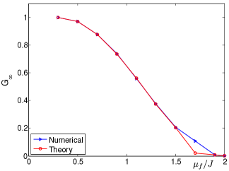
Figure 9: Long-time asymptotic Majorana edge-mode correlation $G_{\infty}$ (23) as a function of the post-quench chemical potential $\mu_{f}$, when a Kitaev Hamiltonian is globally quenched from $H(\mu_{0})$ to $H(\mu_{f})$, with $|\mu_{0}|,|\mu_{f}|\lesssim 2J$. Blue line - numerics, red line - Eq. (25). We take $\mu_{0}=0.3J$, $N=134$, $\Delta=0.72J$.

In the Majorana basis, Eq. (23) can be written as $G_{\infty}=\sum_{i,l=1}^{2N}f^{(0)}_{L,i}f^{(0)}_{R,l}G^{\infty}_{il}$, with $G^{\infty}_{il}=\lim_{t\rightarrow+\infty}-i\langle c_{i}c_{l}\rangle$, and $f^{(0)}_{L/R,l}$ describes left (right) Majorana modes of the initial Hamiltonian. As an illustration, we calculate $G^{\infty}_{il}$ for $i=2j_{1}-1$ and $l=2j_{2}$ with $j_{1}\sim 1$ (near the left edge) and $j_{2}\sim N$ (near the right edge) such that $c_{2j_{1}-1}=a_{j_{1}}+a_{j_{1}}^{{\dagger}}$ and $c_{2j_{2}}=-i(a_{j_{2}}-a_{j_{2}}^{{\dagger}})$. Using Bogoliubov transformation $a_{j}=\sum_{\mu}u_{j\mu}\beta_{\mu}+\nu_{j\mu}^{\ast}\beta_{\mu}^{{\dagger}}$, we diagonalize the post-quench Hamiltonian $H(\mu_{f})$ as $H(\mu_{f})=\sum_{\mu}\epsilon_{\mu}\beta_{\mu}^{{\dagger}}\beta_{\mu}$ (up to unimportant constant) with $\beta_{\nu}$ being the quasi-particle operators for the Hamiltonian $H(\mu_{f})$. With this we obtain $e^{iH(\mu_{f})t}a_{j}e^{-iH(\mu_{f})t}=\sum_{\mu}u_{j\mu}\beta_{\mu}e^{-i\epsilon_{\mu}t}+\nu_{j\mu}^{\ast}\beta_{\mu}^{{\dagger}}e^{i\epsilon_{\mu}t}$, and similarly for $e^{iH(\mu_{f})t}a_{j}^{{\dagger}}e^{-iH(\mu_{f})t}$. After substituting this into the expression for $G^{\infty}_{il}$, and neglecting oscillating terms (the ones containing $\beta_{\mu}\beta_{\nu}$, $\beta_{\nu}^{{\dagger}}\beta_{\mu}^{{\dagger}}$, and $\beta_{\mu}^{{\dagger}}\beta_{\nu}$ with $\mu\neq\nu$) which are averaged to zero after times larger than inverse band-width, we obtain

$$G^{\infty}_{2j_{1}-1,2j_{2}}\approx-\sum_{\mu}\left(A_{j_{1}j_{2}\mu}\langle 0|\beta_{\mu}^{\dagger}\beta_{\mu}|0\rangle+B_{j_{1}j_{2}\mu}\langle 0|\beta_{\mu}\beta_{\mu}^{\dagger}|0\rangle\right),$$

with $A_{j_{1}j_{2}\mu}=(u_{j_{1}\mu}^{\ast}+\upsilon_{j_{1}\mu}^{\ast})u_{j_{2}\mu}+(\upsilon_{j_{1}\mu}+u_{j_{1}\mu})u_{j_{2}\mu}^{\ast}$ and $B_{j_{1}j_{2}\mu}=(u_{j_{1}\mu}+\upsilon_{j_{1}\mu})\upsilon_{j_{2}\mu}^{\ast}+(\upsilon_{j_{1}\mu}^{\ast}+u_{j_{1}\mu}^{\ast})\upsilon_{j_{2}\mu}$. To calculate the correlations in the above expression, we use the second Bogoliubov transformation $a_{j}=\sum_{\sigma}u_{j\sigma}^{(0)}\alpha_{\sigma}+\nu_{j\sigma}^{(0)\ast}\alpha_{\sigma}^{{\dagger}}$ which diagonalizes the initial Hamiltonian as $H(\mu_{0})=\sum_{\sigma}\epsilon_{\sigma}\alpha_{\sigma}^{{\dagger}}\alpha_{\sigma}$ (again up to unimportant constant) in terms of quasiparticles operators $\alpha_{\sigma}$ ($\alpha_{\sigma}^{{\dagger}}$), such that $\alpha_{\sigma}|0\rangle=0$. Then, by virtue of the relation $\beta_{\mu}=\sum_{\sigma}C_{\mu\sigma}\alpha_{\sigma}+D_{\mu\sigma}^{\ast}\alpha_{\sigma}^{{\dagger}}$, with $C_{\mu\sigma}=\sum_{j}u_{j\mu}^{\ast}u_{j\sigma}^{(0)}+\upsilon_{j\mu}^{\ast}\upsilon_{j\sigma}^{(0)}$ and $D_{\mu\sigma}=\sum_{j}u_{j\mu}\upsilon_{j\sigma}^{(0)}+\upsilon_{j\mu}u_{j\sigma}^{(0)}$, we arrive at

$$G^{\infty}_{2j_{1}-1,2j_{2}}=-\sum_{\mu}\Big{(}A_{j_{1}j_{2}\mu}\sum_{\sigma}|D_{\mu\sigma}|^{2}+B_{j_{1}j_{2}\mu}\sum_{\sigma}|C_{\mu\sigma}|^{2}\Big{)}.$$ (24)

Equation (24) contains contributions from both the edge ($\mu=M$) and bulk modes ($\mu\neq M$) of $H(\mu_{f})$ ($|\mu_{f}|\lesssim 2J$). Due to the gapped energy spectrum, the bulk contribution (modes with $\mu\neq M$) to the correlations between the edges are exponentially suppressed, and therefore can be ignored in Eq. (24) in the thermodynamic limit. On the other hand, for the edge contribution ($\mu=M$), we use Majorana wave functions $g_{L/R,j}$ of Hamiltonian $H(\mu_{f})$ in the fermionic representation: $g_{L,j}=u_{jM}+\upsilon_{jM}$ and $g_{R,j}=u_{jM}-\upsilon_{jM}$. Keeping in mind the localization character of the Majoranas at edges, we have $A_{j_{1}j_{2}M}\approx g_{L,j_{1}}g_{R,j_{2}}$ and $B_{j_{1}j_{2}M}\approx-g_{L,j_{1}}g_{R,j_{2}}$. Equation (24) is then simplified as $G^{\infty}_{2j_{1}-1,2j_{2}}\approx g_{L,j_{1}}g_{R,j_{2}}\sum_{\sigma}\Big{(}|C_{M\sigma}|^{2}-|D_{M\sigma}|^{2}\Big{)}$. This expression further involves contributions from the edge $\sigma=M$ and bulk modes $\sigma\neq M$ of initial Hamiltonian $H(\mu_{0})$. For same reasons discussed earlier, we ignore the exponential small bulk contributions ($\sigma\neq M$). For the rest edge contribution ($\sigma=M$), we write $u_{jM}^{(0)}=(1/2)(g_{L,j}^{(0)}+g_{R,j}^{(0)})$ and $\upsilon_{jM}^{(0)}=(1/2)(g_{L,j}^{(0)}-g_{R,j}^{(0)})$ with $g_{L/R,j}^{(0)}$ the initial Majorana wave functions of Hamiltonian $H(\mu_{0})$ in the fermionic basis. Thus by using $C_{MM}=\frac{1}{2}\sum_{j}\Big{(}g_{L,j}g_{L,j}^{(0)}+g_{R,j}g_{R,j}^{(0)}\Big{)}$ and $D_{MM}=\frac{1}{2}\sum_{j}\Big{(}g_{L,j}g_{L,j}^{(0)}-g_{R,j}g_{R,j}^{(0)}\Big{)}$, we find

$$G^{\infty}_{2j_{1}-1,2j_{2}}\approx g_{L,j_{1}}g_{R,j_{2}}\Big{[}\sum_{j=1}^{N}g_{L,j_{1}}g_{L,j_{1}}^{(0)}\Big{]}\Big{[}\sum_{j=1}^{N}g_{R,j_{2}}g_{R,j_{2}}^{(0)}\Big{]}.$$

Calculations of other components of $G^{\infty}_{il}$ are similar, and we finally get

$$G_{\infty}=\Big{[}\sum_{j=1}^{N}g_{L,j}g_{L,j}^{(0)}\Big{]}^{2}\Big{[}\sum_{j=1}^{N}g_{R,j}g_{R,j}^{(0)}\Big{]}^{2}.$$ (25)

We see that, after the quench, the Majorana edge correlation in the long time approaches an asymptotic value, which is determined only by the overlap between the wavefunctions of the Majorana edge modes of $H(\mu_{0})$ and $H(\mu_{f})$ (i.e. $g_{L/R,j}^{(0)}$ and $g_{L/R,j}$). Figure 9 shows numerical results for $G_{\infty}$ (blue curve) as a function of $\mu_{f}$, which are compared to predictions from Eq. (25) (red curve). A good agreement is clearly found, with deviations only appear near the critical point when the energy gap becomes small. We thus conclude that Majorana edge correlations relax to a finite value after a quench within the topological phase, which decreases with $\mu_{f}$ in the post-quench Hamiltonian and eventually varnishes for $\mu_{f}=2J$.

References

- (1) M. König, S. Wiedmann, C. Brüne, A. Roth, H. Buhmann, L. W. Molenkamp, X. L. Qi, and S. C. Zhang, Quantum spin Hall insulator state in HgTe quantum wells, Science 318, 766 (2007).
- (2) D. Hsieh, D. Qian, L. Wray, Y. Xia, Y. S. Hor, R. J. Cava, and M. Z. Hasan, A topological Dirac insulator in a quantum spin Hall phase, Nature (London) 452, 970 (2008).
- (3) Y. L. Chen, J. G. Analytis, J. H. Chu, Z. K. Liu, S. K. Mo, X. L. Qi, H. J. Zhang, D. H. Lu, X. Dai, Z. Fang, S. C. Zhang, I. R. Fisher, Z. Hussain, and Z. X. Shen, Experimental realization of a three-dimensional topological insulator , Science 325, 178 (2009).
- (4) M. Atala, M. Aidelsburger, J. T. Barreiro, D. Abanin, T. Kitagawa, E. Demler, and I. Bloch, Direct measurement of the Zak phase in topological Bloch bands, Nat. Phys. 9, 795 (2013).
- (5) N. Goldman, J. Dalibard, A. Dauphin, F. Gerbier, M. Lewenstein, P. Zoller, and I. B. Spielman, Direct imaging of topological edge states in cold-atom systems, Proc. Natl. Acad. Sci. U. S. A. 110, 6736 (2013).
- (6) G. Jotzu, M. Messer, R. Desbuquois, M. Lebrat, T. Uehlinger, D. Greif, and T. Esslinger, Experimental realization of the topological Haldane model with ultracold fermions, Nature (London) 515, 237 (2014).
- (7) L. Duca, T. Li, M. Reitter, I. Bloch, M. Schleier-Smith, and U. Schneider, An Aharonov-Bohm interferometer for determining Bloch band topology, Science 347, 288 (2015).
- (8) M. Mancini, G. Pagano, G. Cappellini, L. Livi, M. Rider, J. Catani, C. Sias, P. Zoller, M. Inguscio, M. Dalmonte, and L. Fallani, Observation of chiral edge states with neutral fermions in synthetic Hall ribbons, arXiv:1502.02495v1.
- (9) B. K. Stuhl, H. I. Lu, L. M. Aycock, D. Genkina, and I. B. Spielman, Visualizing edge states with an atomic Bose gas in the quantum Hall regime, arXiv:1502.02496v1.
- (10) X. G. Wen, Quantum field theory of many-body systems: from the origin of sound to an origin of light and electrons, (Oxford University Press, New York, 2004).
- (11) M. Z. Hasan and C. L. Kane, Topological insulators, Rev. Mod. Phys. 82, 3045 (2010).
- (12) X. L. Qi and S. C. Zhang, Topological insulators and superconductors, Rev. Mod. Phys. 83, 1057 (2011).
- (13) A. Kitaev, Fault-tolerant quantum computation by anyons, Ann. Phys. 303, 2 (2003).
- (14) S. Das Sarma, M. Freedman, and C. Nayak, Topologically protected qubits from a possible non-Abelian fractional quantum Hall state, Phys. Rev. Lett. 94, 166802 (2005).
- (15) C. Nayak, S. H. Simon, A. Stern, M. Freedman, and S. Das Sarma, Non-Abelian anyons and topological quantum computation, Rev. Mod. Phys. 80, 1083 (2008).
- (16) J. K. Pachos, Introduction to Topological Quantum Computation (Cambridge University Press, Cambridge, 2012).
- (17) J. Alicea and A. Stern, Designer non-Abelian anyon platforms: from Majorana to Fibonacci, arXiv:1410.0359v1.
- (18) A. Kitaev, Unpaired Majorana fermions in quantum wires, Physics-Uspekhi 44, 131 (2001).
- (19) D. A. Ivanov, Non-Abelian statistics of half-quantum vortices in p-wave superconductors, Phys. Rev. Lett. 86, 268 (2001).
- (20) J. Alicea, Y. Oreg, G. Refael, F. von Oppen, and M. P. A. Fisher, Non-Abelian statistics and topological quantum information processing in 1D wire networks, Nat. Phys. 7, 412 (2011).
- (21) F. Wilczek, Majorana returns, Nat. Phys. 5, 614 (2009).
- (22) J. Alicea, New directions in the pursuit of Majorana fermions in solid state systems, Rep. Prog. Phys. 75, 076501 (2012)
- (23) C. W. J. Beenakker, Search for majorana fermions in superconductors, Annu. Rev. Con. Mat. Phys. 4, 113 (2013)
- (24) S. Das Sarma, M. Freedman, and C. Nayak, Majorana zero modes and topological quantum computation, arXiv:1501.02813v2.
- (25) J. D. Sau, R. M. Lutchyn, S. Tewari, and S. Das Sarma, Generic new platform for topological quantum computation using semiconductor heterostructures, Phys. Rev. Lett. 104, 040502 (2010).
- (26) R. M. Lutchyn, J. D. Sau, and S. Das Sarma, Majorana fermions and a topological phase transition in semiconductor-superconductor heterostructures, Phys. Rev. Lett. 105, 077001 (2010).
- (27) J. Alicea, Majorana fermions in a tunable semiconductor device, Phys. Rev. B 81, 125318 (2010).
- (28) Y. Oreg, G. Refael, and F. von Oppen, Helical liquids and Majorana bound states in quantum wires, Phys. Rev. Lett. 105, 177002 (2010).
- (29) B. I. Halperin, Y. Oreg, A. Stern, G. Refael, J. Alicea, and F. von Oppen, Adiabatic manipulations of Majorana fermions in a three-dimensional network of quantum wires, Phys. Rev. B 85, 144501 (2012).
- (30) A. Romito, J. Alicea, G. Refael, and F. von Oppen, Manipulating Majorana fermions using supercurrents, Phys. Rev. B 85, 020502(R) (2012).
- (31) V. Mourik, K. Zuo, S. M. Frolov, S. R. Plissard, E. P. A. M. Bakkers, and L. P. Kouwenhoven, Signatures of Majorana fermions in hybrid superconductor-semiconductor nanowire devices, Science 336, 1003 (2012).
- (32) M. T. Deng, C. L. Yu, G. Y. Huang, M. Larsson, P. Caroff, and H. Q. Xu, Anomalous zero-bias conductance peak in a Nb-InSb nanowire-Nb hybrid device, Nano Lett. 12, 6414 (2012).
- (33) L. P. Rokhinson, X. Y. Liu, and J. K. Furdyna, The fractional ac Josephson effect in a semiconductors-uperconductor nanowire as a signature of Majorana particles, Nat. Phys. 8, 795 (2012).
- (34) A. Das, Y. Ronen, Y. Most, Y. Oreg, M. Heiblum, and H. Shtrikman, Zero-bias peaks and splitting in an Al-InAs nanowire topological superconductor as a signature of Majorana fermions, Nat. Phys. 8, 887 (2012).
- (35) H. O. H. Churchill, V. Fatemi, K. Grove-Rasmussen, M. T. Deng, P. Caroff, H. Q. Xu, and C. M. Marcus, Superconductor-nanowire devices from tunneling to the multichannel regime: zero-bias oscillations and magnetoconductance crossover, Phys. Rev. B 87, 241401(R) (2013).
- (36) A. D. K. Finck, D. J. Van Harlingen, P. K. Mohseni, K. Jung, and X. Li, Anomalous modulation of a zero-bias peak in a hybrid nanowire-superconductor device, Phys. Rev. Lett. 110, 126406 (2013).
- (37) S. Nadj-Perge, I. K. Drozdov, J. Li, H. Chen, S. Jeon, J. Seo, A. H. MacDonald, B. A. Bernevig, and A. Yazdani, Observation of Majorana fermions in ferromagnetic atomic chains on a superconductor, Science 346, 602 (2014).
- (38) L. Jiang, T. Kitagawa, J. Alicea, A. R. Akhmerov, D. Pekker, G. Refael, J. I. Cirac, E. Demler, M. D. Lukin, and P. Zoller, Majorana fermions in equilibrium and in driven cold-atom quantum wires, Phys. Rev. Lett. 106, 220402 (2011).
- (39) S. Nascimbène, Realizing one-dimensional topological superfluids with ultracold atomic gases, J. Phys. B: At. Mol. Opt. Phys. 46, 134005 (2013).
- (40) M. Sato, Y. Takahashi, and S. Fujimoto, Non-Abelian topological order in -wave superfluids of ultracold fermionic atoms, Phys. Rev. Lett. 103, 020401 (2009).
- (41) S. Diehl, E. Rico, M. A. Baranov, and P. Zoller, Topology by dissipation in atomic quantum wires, Nat. Phys. 7, 971 (2011).
- (42) C. V. Kraus, S. Diehl, P. Zoller, and M. A. Baranov, Preparing and probing atomic Majorana fermions and topological order in optical lattices, New J. Phys. 14, 113036 (2012).
- (43) C. V. Kraus, M. Dalmonte, M. A. Baranov, A. M. Läuchli, and P. Zoller, Majorana edge states in atomic wires coupled by pair hopping, Phys. Rev. Lett. 111, 173004 (2013).
- (44) C. V. Kraus, P. Zoller, and M. A. Baranov, Braiding of atomic Majorana fermions in wire networks and Implementation of the Deutsch-Jozsa Algorithm, Phys. Rev. Lett. 111, 203001 (2013).
- (45) C. Laflamme, M. A. Baranov, P. Zoller, and C. V. Kraus, Hybrid topological quantum computation with Majorana fermions: a cold-atom setup, Phys. Rev. A 89, 022319 (2014).
- (46) A. Bühler, N. Lang, C. V. Kraus, G. Möller, S. D. Huber, and H. P. Büchler, Majorana modes and p-wave superfluids for fermionic atoms in optical lattices, Nat. Commun. 5, 4504 (2014)
- (47) G. Goldstein and C. Chamon, Decay rates for topological memories encoded with Majorana fermions, Phys. Rev. B 84, 205109 (2011).
- (48) J. C. Budich, S. Walter, and B. Trauzettel, Failure of protection of Majorana based qubits against decoherence, Phys. Rev. B 85, 121405 (2012).
- (49) D. Rainis and D. Loss, Majorana qubit decoherence by quasiparticle poisoning, Phys. Rev. B 85, 174533 (2012).
- (50) F. L. Pedrocchi and D. P. DiVincenzo, Majorana braiding with thermal noise, arXiv:1505.03712v1.
- (51) Y. Hu and M. A. Baranov, Effects of fluctuations on Majorana edge modes in atomic topological Kitaev wire with molecular reservoir, arXiv:1412.2547v1.
- (52) A. Grishin, I. V. Yurkevich, and I. V. Lerner, Low-temperature decoherence of qubit coupled to background charges, Phys. Rev. B 72, 060509 (R) (2005).
- (53) Y. M. Galperin, B. L. Altshuler, J. Bergli, and D. V. Shantsev, Non-gaussian low-frequency noise as a source of qubit decoherence, Phys. Rev. Lett. 96, 097009 (2006).
- (54) B. Cheng, Q. H. Wang, and R. Joynt, Transfer matrix solution of a model of qubit decoherence due to telegraph noise, Phys. Rev. A 78, 022313 (2008).
- (55) P. Avan and C. Cohen-Tannoudji, Two-level atom saturated by a fluctuating resonant laser beam - calculation of the fluorescence spectrum, J. Phys. B: At. Mol. Opt. Phys. 10, 155 (1977).
- (56) G. Roati, C. D’Errico, L. Fallani, M. Fattori, C. Fort, M. Zaccanti, G. Modugno, M. Modugno and M. Inguscio, Anderson localization of a non-interacting Bose-Einstein condensate, Nature (London) 453, 895 (2008).
- (57) J. Billy, V. Josse, Z. Zuo, A. Bernard, B. Hambrecht, P. Lugan, D. Clément, L. Sanchez-Palencia, P. Bouyer, and A. Aspect, Direct observation of Anderson localization of matter waves in a controlled disorder, Nature (London) 453, 891 (2008).
- (58) C. Gardiner, Stochastic Methods: A Handbook for the Natural and Social Sciences (Springer Berlin Heidelberg, 2010).
- (59) N. G. Van Kampen, Stochastic differential equations, Phys. Rep. 24, 171 (1976).
- (60) P. W. Anderson, Absence of diffusion in certain random lattices, Phys. Rev. 109, 1492 (1958).
- (61) A. Pal and D. A. Huse, Many-body localization phase transition, Phys. Rev. B 82, 174411 (2010).
- (62) P. Zoller, G. Alber, and R. Salvador, Ac Stark splitting in intense stochastic driving fields with Gaussian statistics and non-Lorentzian line shape, Phys. Rev. A 24, 398 (1981).
- (63) P. Facchi and S. Pascazio, Quantum zeno dynamics: mathematical and physical aspects, J. Phys. A: Math. Theor. 41, 493001 (2008).
- (64) A. J. Daley, C. Kollath, U. Schollwöck, and G. Vidal, Time-dependent density-matrix renormalization-group using adaptive effective Hilbert spaces, J. Stat. Mech.: Theory Exp. (2004) P04005.
- (65) U. Schollwöck, The density-matrix renormalization group, Rev. Mod. Phys. 77, 259 (2005).