$\bar{B}\to\bar{K}\pi\ell\ell$ in and outside the $\bar{K}^{*}$ window

Abstract

We study the impact of $\bar{B}\to\bar{K}\pi\ell\ell$ decays on $\bar{B}\to\bar{K}^{*}(\to\bar{K}\pi)\ell\ell$, taking into account the $\bar{K}^{*}$ at finite width. Interference effects can generically be sizable, up to ${\cal{O}}(10\%)$, but are reduced in several ratios of observables of the angular distribution. Information on strong phases is central to control interference effects, which cannot be removed by sideband subtractions. We point out ways to probe the strong phases; only a single one is required to describe leading effects in the region of low hadronic recoil. We find that recent LHCb data on the $\bar{B^{0}}\to\bar{K}^{*0}\mu\mu$ angular observables at low recoil are in good agreement with the standard model.

I Introduction

The semileptonic flavor-changing neutral-current decay $\bar{B}\to\bar{K}^{*}\ell\ell$ is one of the key modes at current and future high luminosity flavor facilities. If analyzed through the quasi-4-body $\bar{B}\to\bar{K}\pi\ell\ell$ decays, several observables can be obtained that allow to precisely probe flavor physics in the standard model (SM) and beyond.

With increasing experimental precision further backgrounds become of importance. In fact the shape of the $\bar{B}\to\bar{K}^{*}(\to\bar{K}\pi)\ell\ell$ angular distribution is distorted by non-resonant $\bar{B}\to\bar{K}\pi\ell\ell$ decays as well as resonances decaying to $\bar{K}\pi$. Building on previous works Das:2014sra we study the impact of such backgrounds, taking into account the $\bar{K}^{*}$ at finite width. Since the sole suppression of the non-resonant $\bar{B}\to\bar{K}\pi\ell\ell$ mode relative to $\bar{B}\to\bar{K}^{*}\ell\ell$ is due to phase space, generically sizable interference effects of order $1/(4\pi)$ are expected. Non-resonant decays have dominant S- and P-wave components; the leading background stems therefore from P-P and S-P interference. Only the latter can be separated from $\bar{B}\to\bar{K}^{*}\ell\ell$ by its different angular structure. The contamination from resonant $\bar{K}\pi$ contributions in an S-wave, as originating from $\bar{B}\to\bar{\kappa}(800)\ell\ell$ and $\bar{B}\to\bar{K}_{0}(1430)\ell\ell$ decays, has been previously considered in Becirevic:2012dp ; Blake:2012mb ; Matias:2012qz ; Doring:2013wka .

We work in the region of low hadronic recoil, which is advantageous due to the suppression of $1/m_{b}$ power corrections Grinstein:2004vb ; Bobeth:2010wg ; Beylich:2011aq and its direct accessibility to form factor calculations based on lattice QCD Horgan:2013hoa and heavy hadron chiral perturbation theory (HH$\chi$PT), e.g., Refs. Burdman:1992gh ; Lee:1992ih .

The relative strong phases between the $\bar{K}^{*}$ and its backgrounds can in principle be probed experimentally using interference. An important feature of the $\bar{B}\to\bar{K}\pi\ell\ell$ decay is that it gives access to new combinations of short-distance coefficients that are not present in the $\bar{K}^{*}$ signal mode Das:2014sra . We discuss resulting opportunities for reducing the background and for probing new physics.

The paper is organized as follows: We give details on the finite width implementation of the $\bar{K}^{*}$ in Sec. II. In Sec. III we estimate the backgrounds to $\bar{B}\to\bar{K}^{*}(\to\bar{K}\pi)\ell\ell$ for relevant observables. In Sec. IV we show how to probe strong phases with ratios of angular observables and discuss SM tests and beyond the SM (BSM) searches with SM-nulltests. In Sec. V we compare SM predictions to the latest preliminary LHCb findings for $\bar{B^{0}}\to\bar{K}^{*0}\mu\mu$ angular observables based on $3\,{\rm fb}^{-1}$ LHCb:2015dla . In Sec. VI we conclude. In several appendices we give auxiliary information.

II Framework

The $\bar{B}\to\bar{K}\pi\ell\ell$ decay amplitudes $H_{0,\parallel,\perp}^{L/R}$ factorize in the operator product expansion (OPE) Buchalla:1998mt ; Grinstein:2004vb at leading order in $1/Q$, $Q=\left\{m_{b},\sqrt{q^{2}}\right\}$, into universal short-distance coefficients $C_{\pm}^{L/R}$ and form factors (see Ref. Das:2014sra for details),

$$H_{0,\parallel}^{L/R}=C_{-}^{L/R}(q^{2})\cdot\mathcal{F}_{0,\parallel}(q^{2},p^{2},\cos\theta_{K})\;,\quad H_{\perp}^{L/R}=C_{+}^{L/R}(q^{2})\cdot\mathcal{F}_{\perp}(q^{2},p^{2},\cos\theta_{K})\;.$$ (1)

The contributions from various hadronic final states are contained in the generalized transversity form factors

$${\cal F}_{0} \equiv{\cal F}_{0}\left(q^{2},p^{2},\cos\theta_{K}\right)=F_{0}\left(q^{2},p^{2},\cos\theta_{K}\right)+\sum_{R}P^{0}_{J_{R}}(\cos\theta_{K})\cdot F_{0J_{R}}\left(q^{2},p^{2}\right)\,,$$ (2)

$${\cal F}_{i} \equiv{\cal F}_{i}\left(q^{2},p^{2},\cos\theta_{K}\right)=F_{i}\left(q^{2},p^{2},\cos\theta_{K}\right)+\sum_{R}\frac{P^{1}_{J_{R}}(\cos\theta_{K})}{\sin\theta_{K}}\cdot F_{iJ_{R}}\left(q^{2},p^{2}\right)\,,\quad i=\parallel,\perp\,.$$

Here, the first terms $F_{0,\|,\perp}$ on the right-hand side correspond to the non-resonant $\bar{B}\to\bar{K}\pi$ transversity form factors (cf. App. C), whereas the second terms containing the form factors $F_{(0,\|,\perp)R}$ belong to resonant states $R$ with spin $J_{R}$ decaying to $\bar{K}\pi$. The $P^{m}_{\ell}$ are the associated Legendre polynomials. In this work $q^{2}$ and $p^{2}$ denote the invariant mass squared of the dilepton- and $\bar{K}\pi$-system, respectively. $\theta_{K}$ is the angle between the kaon and the $\bar{B}$ in the $\bar{K}\pi$ center-of-mass system.

In our numerical estimate we employ the $\bar{B}\to\bar{K}\pi$ form factors from HH$\chi$PT, given in Eq. (26). Sizable uncertainties are present in these leading order results, already parametrically from the HH$\chi$PT coupling constant, $g$ ($g^{2}$) in $F_{0,\parallel}$ ($F_{\perp}$) of $13\%$ ($26\%$), in addition to higher-order corrections. The expansion is expected to work better towards zero recoil. Alternative determinations for $\bar{B}\to\bar{K}\pi$ form factors are desirable.

For $\bar{B}\to\bar{K}^{*}\ell\ell$ decays, it is useful to match the corresponding P-wave contributions $F_{(0,\|,\perp)P}=F_{(0,\|,\perp)P}(q^{2},p^{2})$ onto the common $\bar{B}\to\bar{K}^{*}$ transversity form factors $f_{(0,\|,\perp)}(q^{2})$, see App. B for details,

$$F_{0P}= -3f_{0}(q^{2})\,P^{BW}_{K^{*}}(p^{2})\,e^{i\delta_{K^{*}}}\,,\quad F_{\parallel P}=-3\sqrt{\frac{1}{2}}\,f_{\parallel}(q^{2})\,P^{BW}_{K^{*}}(p^{2})\,e^{i\delta_{K^{*}}}\,,\quad F_{\perp P}=3\sqrt{\frac{1}{2}}\,f_{\perp}(q^{2})\,P^{BW}_{K^{*}}(p^{2})\,e^{i\delta_{K^{*}}}\,.$$ (3)

Here we included factors $e^{i\delta_{K^{*}}}$ to account for a relative strong phase $\delta_{K^{*}}$ between the $\bar{K}^{*}$ and the non-resonant contributions. In general it can assume values between $-\pi$ and $+\pi$. Eq. (1) implies that there is only one universal strong phase for all transversity amplitudes between the $\bar{K}^{*}$ and its non-resonant background. The strong phase should vary with $p^{2}$, and this could be taken into account given knowledge of the functional form. By keeping in this work $\delta_{K^{*}}$ constant in each $p^{2}$-integration window it becomes an effective $p^{2}$-bin specific phase.

As explicitly shown in Ref. Das:2014sra , the non-resonant background dominates over the one from the scalar mesons $\kappa(800)$ and $\bar{K}_{0}(1430)$ in the $\bar{B}\to\bar{K}^{*}\ell\ell$ dilepton mass distribution. Since in addition the fraction of states with longitudinal polarization $F_{L}$ from purely non-resonant decays at low recoil is large, $\sim 0.5$ Das:2014sra , the contributions from S-wave resonances are subdominant also in this observable. In the angular coefficients $I_{3..9}$, S-wave contributions can be isolated with an angular analysis or are even absent. We therefore consider the non-resonant $\bar{K}\pi$ decays as an effective model for the background. We note, however, that this can be refined as resonance contributions can be modeled in a straightforward manner, at the price of additional phases and parametric uncertainties. In the remainder of this work we denote by $\bar{B}\to\bar{K}\pi\ell\ell$ decays originating from the $\bar{K}^{*}$ as well as non-resonant modes, including interference, unless stated otherwise.

We incorporate the finite width of the $\bar{K}^{*}$ by the usual Breit-Wigner (BW) lineshape,

$$P_{K_{J}}^{BW}(p^{2})=\sqrt{\frac{m_{K_{J}}\Gamma_{K_{J}}}{\pi}}\frac{1}{p^{2}-m_{K_{J}}^{2}+im_{K_{J}}\Gamma_{K_{J}}(p^{2})}\,,\quad{\rm with}\quad\int dp^{2}|P_{K_{J}}^{BW}(p^{2})|^{2}=1\,,$$ (4)

$m_{K_{J}}$ and $\Gamma_{K_{J}}$ being the mass and mean width of the resonance $K_{J}$ with spin $J$, respectively. We further take into account the running width of the $\bar{K}^{*}$:

$$\Gamma_{K^{*}}(p^{2})=\Gamma_{K^{*}}^{0}\left(\frac{p^{*}}{p^{*}_{0}}\right)^{3}\frac{m_{K^{*}}}{\sqrt{p^{2}}}\frac{1+(r_{BW}\,p^{*}_{0})^{2}}{1+(r_{BW}\,p^{*})^{2}}\,,\quad\rm{where}$$ (5)

$$p^{*}=\frac{\sqrt{\lambda_{p}}}{2\sqrt{p^{2}}}\,,\quad p^{*}_{0}=p^{*}|_{p^{2}=m_{K^{*}}^{2}}\,,\quad\lambda_{p}=\lambda(p^{2},m_{K}^{2},m_{\pi}^{2})\,,$$ (6)

with the Blatt-Weisskopf parameter $r_{BW}$ (see Table 2 for numerical input) and the common phase space function $\lambda(a,b,c)=a^{2}+b^{2}+c^{2}-2(ab+ac+bc)$. Other $\bar{K}^{*}$-lineshapes may also be studied, however, in view of the current experimental precision and the form factor uncertainties we refrain in this work from doing so. We remark that experimental information on the lineshape in the kinematical situation relevant here could be obtained from angular studies in $\bar{B}_{s}\to\bar{K}^{*}(\to\bar{K}\pi)\ell\nu$ decays.

The invariant-mass cuts suitable for $\bar{B}\to\bar{K}^{*}\ell\ell$ experimental studies are taken from Ref. Das:2014sra , which we follow closely:

$$0.64\,\mbox{GeV}^{2}<p^{2}<1\,\mbox{GeV}^{2}: ~{}~{}~{}~{}P~{}~{}(\bar{K}^{*}\mbox{signal window) cut}\,,$$

$$p^{2}_{\rm min}=0.40\,\mbox{GeV}^{2}<p^{2}<1.44\,\mbox{GeV}^{2}: ~{}S+P~{}(\bar{K}^{*}\mbox{total window) cut}\,,$$ (7)

where $p^{2}_{\rm min}=(m_{K}+m_{\pi})^{2}$.

Upon evaluation of the $\bar{K}^{*}$ at finite width kinematics is affected; notably there will be events above the zero-width endpoint $q^{2}>(m_{B}-m_{K^{*}})^{2}$, where $\lambda_{K^{*}}\equiv\lambda(m_{B}^{2},q^{2},m_{K^{*}}^{2})<0$. To take this fully into account would require, besides enlarging the phase space, taking into account hadronic form factors computed at finite width as well, which are not available presently, see, however, Ref. Briceno:2014uqa . For concreteness, we pursue the following phenomenological avenue: we use $\lambda(m_{B}^{2},q^{2},p^{2})$ instead of $\lambda_{K*}$ in the overall phase space factor (24) of the $\bar{K}^{*}$-contribution, keep $\lambda_{K*}$ elsewhere, in particular in $\bar{B}\to\bar{K}^{*}$ form factors (23), and have the plots end at $\lambda_{K*}=0$ above which the rate dies out anyway. The effects from different treatments around the endpoint are negligible in view of other uncertainties.

III $\bar{B}\to\bar{K}\pi\ell\ell$ distributions

In this section we study the impact of non-resonant $\bar{B}\to\bar{K}\pi\ell\ell$ decays on the $\bar{B}\to\bar{K}^{*}(\to\bar{K}\pi)\ell\ell$ analysis. The background induces in general a shift and a phase-related uncertainty in the observables. We work out the interference effects on the dilepton mass distributions (Sec. III.1), on the fraction of longitudinally polarized $\bar{K}^{*}$, $F_{L}$, (Sec. III.2) and on the angular observables (Sec. III.3). Auxiliary information on the full angular distribution of $\bar{B}\to\bar{K}\pi\ell\ell$ decays has been collected in App. A, and is based on Ref. Das:2014sra to which we refer for further details.

III.1 Dilepton spectrum

In Fig. 1 we show the influence of the interfering non-resonant contribution on the SM differential branching fraction $d{\cal{B}}(\bar{B}\to\bar{K}\pi\ell\ell)/dq^{2}$ in the P-wave ’signal’ window (left) and the S+P total window (mid); in the panel on the right the uncertainties from form factors and parametric inputs are illustrated.

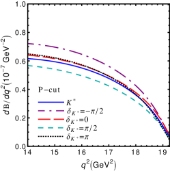
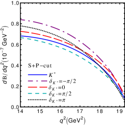
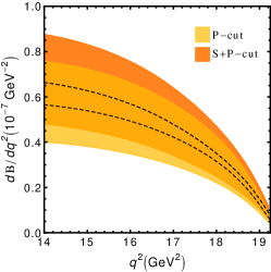
Figure 1: The SM differential branching fraction $d{\cal{B}}(\bar{B}\to\bar{K}\pi\ell\ell)/dq^{2}$ in the P-cut ’signal’ window (left) and the S+P total window (mid) for central values of input and for different values of the strong phase. The solid blue curve corresponds to the resonant $K^{*}$ contribution. All curves are with running width in the Breit-Wigner propagator for the $K^{*}$, c.f. Eq. (5). In the plot to the right the bands correspond to the uncertainties coming from form factors and parametric inputs for fixed strong phase $\delta_{K^{*}}=\pi/2$.

In Fig. 2 we show similarly $d^{2}{\cal{B}}(\bar{B}\to\bar{K}\pi\ell\ell)/dq^{2}dp^{2}$ for fixed $q^{2}=16\,\mbox{GeV}^{2}$, with a zoom into the $K^{*}$ signal region on the right. For $p^{2}\gtrsim 1\,\mbox{GeV}^{2}$ the non-resonant branching ratio becomes comparable to the $\bar{K}^{*}$ one. We note that the numerical difference between using constant or running width (c.f. Eq. (5)) amounts to less than a few percent.

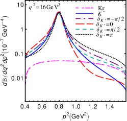
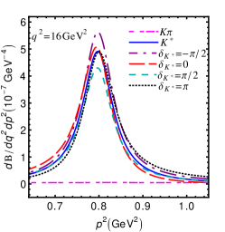
Figure 2: $d^{2}{\cal{B}}(\bar{B}\to\bar{K}\pi\ell\ell)/dq^{2}dp^{2}$ at $q^{2}=16\,\mbox{GeV}^{2}$ in the SM for central values of input and different values of the strong phase. The solid blue curve corresponds to the resonant $K^{*}$, the magenta curve to the purely non-resonant contribution. The plot to the right is a zoom of the left one around the $\bar{K}^{*}$-window.

The spread induced by varying the relative strong phase is considerable. We quantify this in Fig. 3, where we show the fraction of resonant $(\bar{K}^{*})$ to all events,

$$f=\frac{\int dp^{2}d^{2}{\cal{B}}(\bar{B}\to\bar{K}^{*}(\to\bar{K}\pi)\ell\ell)/dq^{2}dp^{2}}{\int dp^{2}d^{2}{\cal{B}}(\bar{B}\to\bar{K}\pi\ell\ell)/dq^{2}dp^{2}}\,,$$ (8)

that is, the denominator includes resonant $\bar{K}^{*}$ and non-resonant decays and their interference. The correction amounts to up to $15\%$, depending on $\delta_{K^{*}}$, and can be even larger in the very $\bar{B}\to\bar{K}^{*}\ell\ell$ endpoint region. Since the sole suppression of the non-resonant $\bar{B}\to\bar{K}\pi\ell\ell$ mode relative to $\bar{B}\to\bar{K}^{*}\ell\ell$ decays is due to phase space, effects of order $1/(4\pi)$ are actually expected. This is presently within the uncertainties of the $\bar{B}\to\bar{K}^{*}\ell\ell$ branching ratio which amount to about 30 percent from form factors and parametric input, see plot to the right in Fig 1. Nevertheless, it stresses the importance of (angular) observables with less sensitivity to hadronic physics. We discuss examples for the latter in the next sections. Notably, even very rough bounds on the strong phase would reduce the uncertainties related to interference. We study this further in Section IV.1.

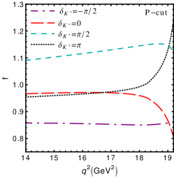
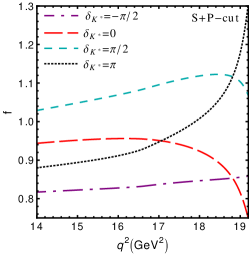
Figure 3: The correction fraction defined in Eq. (8) in the P signal cut window (left) and S+P cut window (right) in the SM for different values of the relative strong phase.

III.2 Longitudinal polarization fraction

The longitudinal polarization fraction, given by

$$F_{L}=\frac{d\Gamma(\bar{B}\to\bar{K}\pi\ell\ell)/dq^{2}\big{|}_{{\cal{F}}_{\perp,\parallel}=0}}{d\Gamma(\bar{B}\to\bar{K}\pi\ell\ell)/dq^{2}}\,,$$ (9)

is shown in Fig. 4. The $\bar{K}\pi$ background shifts $F_{L}$ to larger values by about 6% in the P-cut and $11\%$ in the S+P-cut window, while the uncertainty from the strong phase is only up to $2\%$ in the P-cut and $3\%$ in the S+P-cut window. The shift remains strictly positive even when including the hadronic uncertainties and its size is larger than the present experimental uncertainty for this observable, see Sec. V. The inclusion of this effect is therefore important when interpreting the available data.

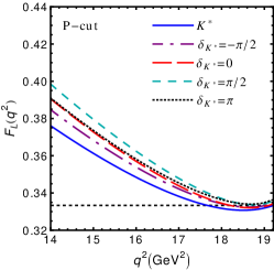
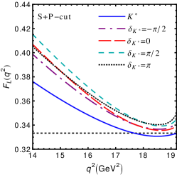
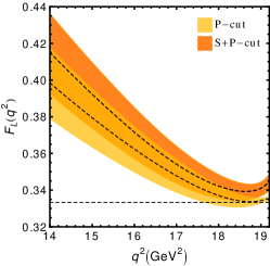
Figure 4: The longitudinal polarization fraction $F_{L}$ in the P-cut ’signal’ window (left) and S+P total window (mid) in the SM for central values and for different values of the strong phase. The solid blue curve corresponds to the resonant $K^{*}$ contribution, the horizontal dotted lines to the endpoint prediction $F_{L}=1/3$. In the plot to the right the bands correspond to the uncertainties coming from form factors and parametric inputs for fixed strong phase $\delta_{K^{*}}=\pi/2$.

III.3 Angular observables

The angular coefficients $I_{i}$ are observables of the $\bar{B}\to\bar{K}\pi\ell\ell$ angular distribution, see Appendix A for a brief overview. It is useful to define integrated angular coefficients $\hat{I}_{i}=\hat{I}_{i}(q^{2})$ as follows:

$$\hat{I}_{i} =\int dp^{2}\int_{-1}^{+1}d\cos\theta_{K}I_{i}(q^{2},p^{2},\cos\theta_{K})\,,\quad i=3,6,9\,,$$

$$\hat{I}_{i} =\int dp^{2}\left[\int_{0}^{+1}-\int_{-1}^{0}\right]d\cos\theta_{K}I_{i}(q^{2},p^{2},\cos\theta_{K})\,,\quad i=4,5,7,8\,.$$ (10)

The relations between the $\hat{I}_{i}$ and the coefficients of the pure P-wave analysis, $J_{i},J_{ic}$ (cf. Ref. Das:2014sra ) read:

$$\hat{I}_{i} =\frac{4}{3}J_{i}+\mbox{pure D-waves and higher}\,,\quad i=3,6,9\,,$$

$$\hat{I}_{i} =\frac{2}{3}J_{ic}+\mbox{D-waves and higher}\,,\quad i=4,5,7,8\,.$$ (11)

The first equation holds up to pure D-wave contributions and higher ones. The second equation receives in addition corrections from S-D wave interference. We recall that the leading contributions of the background are in S- and P-wave. The dominant effect in the $\bar{K}^{*}$-signal window is hence P-P interference. For the $J_{i},J_{ic}$ we follow here the conventions spelled out in Das:2014sra . The relation to the commonly used ones Bobeth:2008ij ; Bobeth:2010wg (BHP) read $J_{i}=3/4J_{i}^{BHP}$ for $i=3,6,9$ and $J_{ic}=3/2J_{i}^{BHP}$ for $i=4,5,7,8$. The $J_{i}$ are building blocks for further observables, often designed to have specific features such as reduced hadronic uncertainties.

To discuss the shift and induced uncertainties related to the interfering backgrounds we define correction fractions

$$\epsilon_{i}=\frac{\hat{I}_{i}(\bar{B}\to\bar{K}^{*}(\to\bar{K}\pi)\ell\ell)}{\hat{I}_{i}(\bar{B}\to\bar{K}\pi\ell\ell)}\,,\quad i=3,4,5,6\,.$$ (12)

As in Eq. (8), the denominators of the $\epsilon_{i}$ include both $\bar{K}^{*}$ and (interfering) non-resonant contributions, whereas in the numerator only the $\bar{K}^{*}$ is included, c.f. Eq. (3). The $\epsilon_{i}$ depend on the cut in $p^{2}$; we employ an identical one for both numerator and denominator.

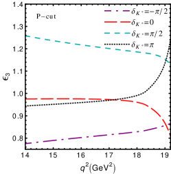
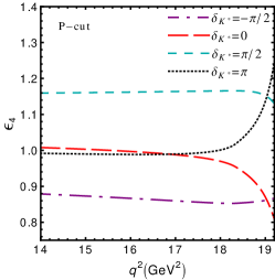
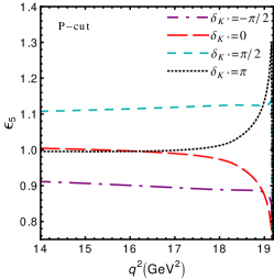
Figure 5: The correction fractions $\epsilon_{3,4,5,6}$, cf. Eq. (12), in the P-signal-cut window in the SM basis for central values and for different values of the strong phase.

As shown in Fig. 5, the corrections are up to 15% for $I_{5,6}$, 20% for $I_{4}$ and 30% for $I_{3}$. The corresponding effects in the S+P cut window are very similar and not shown. The qualitative dependence on the strong phase is in all cases similar and follows the one of the branching ratio, shown in Fig. 3, which drastically reduces the net effect in ratios, as a feature of a universal strong phase. We show this explicitly for the observables

$$S_{i}\equiv\frac{\hat{I}_{i}(\bar{B}\to\bar{K}\pi\ell\ell)}{d\Gamma(\bar{B}\to\bar{K}\pi\ell\ell)/dq^{2}}\,,$$ (13)

where we adopt the notation from $\bar{B}\to\bar{K}^{*}\ell\ell$ studies Altmannshofer:2008dz to allow for easier comparison. Interference affects the observables $S_{5}$ and $A_{\rm FB}=S_{6}$ very little, followed by $S_{4}$ and then $S_{3}$, as can be seen in Fig. 6 for the P-cut window. The uncertainties on the $S_{i}$ from the strong phase are up to 14% on $S_{3}$, while they do not exceed a few percent for $S_{4-6}$. The largest shift from interference receives $S_{4}$, which gets suppressed by about $5\%$ over the whole low recoil region. The shifts in the other angular observables are smaller and vary with $q^{2}$.

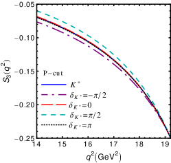
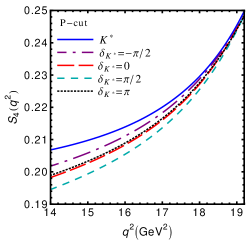
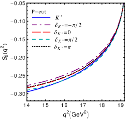
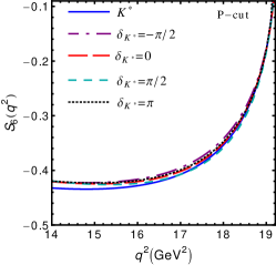
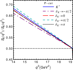
Figure 6: $S_{3,4,5,6}$ as given in Eq. (13) and $S_{5}/S_{6}$ in P signal-cut window in the SM for central values and different values of the strong phase. The solid blue curve corresponds to the resonant $K^{*}$ contribution.

$I_{7,8,9}$ are SM nulltests of the $\bar{K}^{*}$ distribution. This follows from universality i.e., $\bar{K}^{*}$-polarization independence of the short-distance coefficients of the leading-order low-recoil OPE Bobeth:2010wg , which extends to the case with CP violation. For $I_{7}$ this is even true in the more general SM+SM’basis given in Eq. (18) Bobeth:2012vn . However, interference of the $\bar{K}^{*}$ with the non-resonant $\bar{K}\pi$ contribution induces small backgrounds, see Fig. 7, where $\hat{I}_{7,8,9}$ are shown in the SM, normalized to the mean total width $\Gamma(B)$ after P-cut and S+P-cut integration. Comparing their size to the dilepton spectrum shown in Fig. 1, the effect is at most of the order of a few percent and largest for $\hat{I}_{7}$, followed by $\hat{I}_{9}$. The induced values for $|\hat{I}_{7,8,9}^{\rm SM}|$ are largest for $\delta_{K^{*}}$ near $0$ and $\pi$. On the contrary, the largest interference effects in the dilepton spectrum and other ${\rm Re}$-type observables like $I_{3,4,5,6}$ are assumed at $\delta_{K^{*}}\sim\pm\pi/2$. As a result, strong-phase-related uncertainties do not cancel efficiently in ratios $S_{7,8,9}$, and remain sizable, at ${\cal{O}}(1)$.

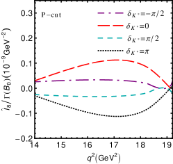
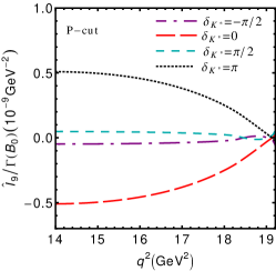
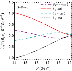
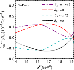
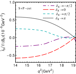
Figure 7: The angular coefficients $\hat{I}_{7,8,9}/\Gamma(B)$ in the SM for different values of the relative strong phase in the P-cut window (upper row) and S+P cut window (lower row).

IV Phenomenlogy

The unknown strong phase $\delta_{K^{*}}$ implies a sizable uncertainty in the SM predictions, see Figs. 1-7, which is very difficult to control theoretically. We therefore start this section by discussing opportunities from $I_{7,8,9}$ for probing strong phases (Sec. IV.1), before discussing BSM physics (Sec. IV.2).

IV.1 Probing strong phases

The ratios

$$\frac{\hat{I}_{7}}{\hat{I}_{5}}\,,\frac{\hat{I}_{7}}{\hat{I}_{6}}\,,\frac{\hat{I}_{8}}{\hat{I}_{3}}\,,\frac{\hat{I}_{8}}{\hat{I}_{4}}\,,\frac{\hat{I}_{9}}{\hat{I}_{3}}\,,\frac{\hat{I}_{9}}{\hat{I}_{4}}\,,S_{8}\,,S_{9}\,,$$ (14)

are all short-distance-free in the SM basis, cf. Eq. (21). They can be used to obtain information on the strong phase between the resonant and non-resonant contributions to $\bar{B}\to\bar{K}^{*}\ell\ell$ decays, since for these ratios the dependence on the strong phase fully remains, as discussed in the previous section. The functional dependence on the strong phase $\delta_{K^{*}}$ varies with the $p^{2}$-cuts as detailed in App. D. We see this leading behaviour explicitly in Fig. 8. It is evident that the observables are sensitive to the strong phase, which can be measured in any of the ratios up to a twofold ambiguity, which could be resolved with a second measurement of a ratio with a different numerator. As stressed already in Sec. II, $\delta_{K^{*}}$ depends on $p^{2}$. Hence, phases extracted using different $p^{2}$-cuts are in general not the same.

The observables in Eq. (14) can be larger outside the $\bar{K}^{*}$-window, where signal and interfering background become more comparable. This is especially the case in the $p^{2}$-region above the $\bar{K}^{*}$, where more phase space is available away from the $\bar{K}^{*}$-peak than below. Being outside the $\bar{K}^{*}$-window comes, however, at the price of fewer events. It would require experimental simulations to estimate the ideal $p^{2}$ cuts for maximal sensitivity; however, note again that the strong phase is expected to vary over $p^{2}$. Theory uncertainties from ratios of the form factors $F_{nr}$ and $F_{K^{*}}$ apply.

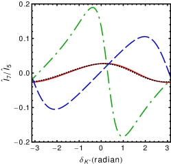
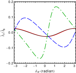
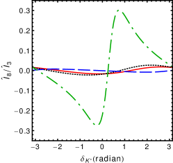
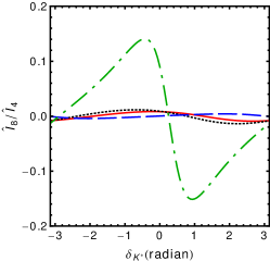
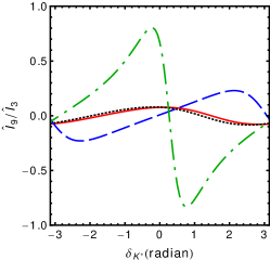
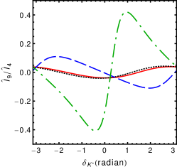
Figure 8: Short-distance-free ratios in the SM basis as in Eq. (14) versus $\delta_{K^{*}}$ at $q^{2}=16\,\mbox{GeV}^{2}$ in the P-cut signal window (red solid), the S+P-cut total window (black dotted), below the signal window, $p^{2}_{\rm min}<p^{2}<0.64\,\mbox{GeV}^{2}$ (blue dashed), and above the signal window, $0.9\,\mbox{GeV}^{2}<p^{2}<2\,\mbox{GeV}^{2}$ (green dash-dotted).

IV.2 Beyond the Standard Model

While a complete exploration of the BSM sensitivity of all angular observables in the full basis in Eq. (20) is beyond the scope of this work, here we concentrate on $I_{7,8,9}$ because i) they are SM nulltests of $\bar{B}\to\bar{K}^{*}(\to\bar{K}\pi)\ell\ell$ decays and ii) they involve new combinations of short-distance coefficients Das:2014sra . Specifically, $\delta\rho$ and ${\rm Re}\rho_{2}^{-}$ can in $\bar{B}\to\bar{K}\pi\ell\ell$ only be accessed with $I_{7}$ and $I_{8,9}$, respectively, see Eq. (18). Note that $\delta\rho$ and ${\rm Re}\rho_{2}^{-}$ can also be probed with $\Lambda_{b}\to\Lambda\ell\ell$ decays Boer:2014kda . A closer look exhibits that there arise new constraints only, if interference arises between i) primed and unprimed Wilson coefficients and ii) contributions from operators with vector and axial vector structure. Given the presence of $C_{9,10}$ in the SM, this requires at least one coefficient $C^{\prime}_{i}\neq 0$ from new physics. Consequently, we focus on exploring the sensitivity to primed operators. We recall that in this paper we do not consider CP violation, as it is consistent with semileptonic and radiative $b\to s$ data to do so and small in the SM. Larger effects in $I_{8,9}$ are of course possible with CP violation, which is driven by ${\rm Re}({\cal{F}}{\cal{F}}^{*})$ rather than its imaginary part; however, this is a feature that can already be probed with $\bar{B}\to\bar{K}^{*}\ell\ell$ decays Bobeth:2008ij ; Bobeth:2012vn . The assumption of negligible CP-violation can be checked by measuring CP-asymmetries Bobeth:2008ij .

Integrating $\hat{I}_{7,8,9}$ in the SM over high $q^{2}$, $15\,\mbox{GeV}^{2}\leq q^{2}\leq 19.2\,\mbox{GeV}^{2}$, in the P-cut window, we find, roughly, cf (33),

$$\int dq^{2}\hat{I}_{(7,8,9)}^{\rm\,SM}(q^{2})/\Gamma(B)\simeq(+1.7,+0.4,-1.4)\cdot 10^{-9}\,\cos\delta_{K^{*}}\,.$$ (15)

Despite the uncertainty from the unknown strong phase, all these observables remain small in the SM; a measurement of a larger value would indicate a non-vanishing BSM contribution.

New physics effects are exemplified in Fig. 9. Since $I_{8}$ and $I_{9}$ involve the same short-distance physics, we only show one of them, $I_{9}$, which can be larger in magnitude. Note, that in the presence of right-handed currents there is even in the CP-limit a non-zero ${\rm Im}\rho_{2}^{+}$ induced by quark loops, so the dependence of $I_{8,9}$ on $C_{7,9}^{\prime}$ is tilted relative to $C_{10}^{\prime}$. Current low recoil data constrain $|S_{7,8,9}|$ to be below the ${\cal{O}}(5-10\%)$ level LHCb:2015dla , about to probe BSM effects.

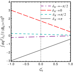
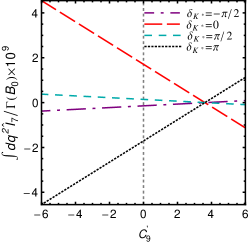
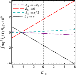
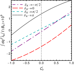
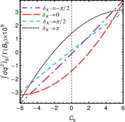
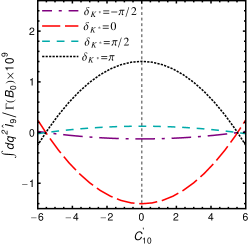
Figure 9: The angular coefficients $\int dq^{2}\hat{I}_{7,9}/\Gamma(B)$ integrated over high-$q^{2}$, $15\,\mbox{GeV}^{2}\leq q^{2}\leq 19.2\,\mbox{GeV}^{2}$, in the P-cut window with one right-handed BSM Wilson coefficient switched on while all others assume SM values. The vertical line corresponds to the SM.

In Fig. 10 we show the resulting contours from a hypothetical SM-like measurement of high-$q^{2}$-integrated $\hat{I}_{7,9}/\Gamma(B^{0})$ in comparison with those from other observables. They demonstrate the complementarity with other observables as well as the need to get contraints on the strong phase: without knowledge of the latter, the whole area between $I_{7,9}$-contours for $\delta_{K^{*}}=0,\pi$ remains viable. Nevertheless, even without this knowledge measurements will allow to exclude a significant part of the parameter space. Of course the determination of these parameters eventually requires a global fit to all $|\Delta B|=|\Delta S|=1$ processes with the strong phase (at low recoil) as additional parameter.

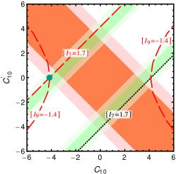
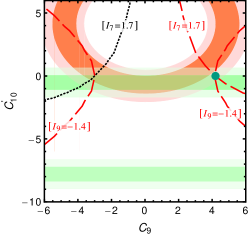
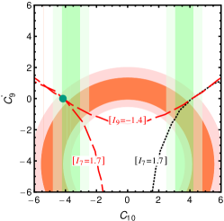
Figure 10: Contours from hypothetical measurements for the high-$q^{2}$-integrated observables $\hat{I}_{7,9}/\Gamma(B^{0})$ (in units of $10^{-9}$) for central values of input versus constraints from present measurements for $\mathcal{B}(B_{s}\to\mu^{+}\mu^{-})$ CMS:2014xfa (green) and $\mathcal{B}(B\to K\mu^{+}\mu^{-})|_{q^{2}\in[1.1,6]{\rm GeV^{2}}}$ Aaij:2014pli (orange) in different $C-C^{\prime}$ planes (Wilson coefficients that are not shown assume SM values). The darker and lighter areas correspond to $1\sigma$ and $2\sigma$, respectively. The contours correspond to conic sections given by the bilinears in Eq. (19). The red dashed (black dotted) curve corresponds to $\delta_{K^{*}}=0\,(\pi)$. The green blob corresponds to the SM.

V Comparison of $\bar{B}\to\bar{K}^{*}\mu\mu$ data with SM predictions

In Table 1 we compare our SM predictions including finite width effects to the recent LHCb data on $\bar{B}\to\bar{K}^{*}\mu\mu$ angular observables LHCb:2015dla . In the latter study S-wave backgrounds have been considered by including S-wave observables explicitly as nuisance parameters. We give therefore additional values in parentheses with the S-wave component, present only in ${\cal{F}}_{0}$, removed by replacing $F_{0}\to F_{0}-\int d\cos\theta_{K}F_{0}/2$, cf. Eq. (25). We use the most reliable bins in the low recoil region: the one with the largest $q^{2}$-interval to allow for maximal smearing, $15<q^{2}<19\,\mbox{GeV}^{2}$, and the one closest to the endpoint, with highest momentum transfer and furthest away from the $c\bar{c}$-threshold, $17<q^{2}<19\,\mbox{GeV}^{2}$. Note the different conventions between the $S_{i}$ used in this work, Eq. (13), and LHCb LHCb:2015dla . For the SM predictions, as usual numerator and denominator are $q^{2}$-integrated before dividing them. In the long run this may not be necessary, as it may be feasible to extract amplitudes without binning Egede:2015kha .

	LHCb$\left[15,19\right]^{a,b}$	SM$\left[15,19\right]$	LHCb$\left[17,19\right]^{a,b}$	SM$\left[17,19\right]$	endpoint
$F_{L}$	$0.344\pm 0.031$	$0.351(0.342)\pm 0.010\pm 0.003$	$0.354\pm 0.054$	$0.338(0.333)\pm 0.006\pm 0.002$	$1/3$
$A_{\rm FB}=S_{6}$	$-0.355\pm 0.029$	$-0.391(-0.396)\pm 0.016\pm 0.005$	$-0.306\pm 0.049$	$-0.349(-0.351)\pm 0.015\pm 0.007$	$0^{c}$
$S_{3}$	$-0.122\pm 0.026$	$-0.129(-0.131)\pm 0.009\pm 0.007$	$-0.145\pm 0.062$	$-0.167(-0.169)\pm 0.007\pm 0.005$	$-1/4$
$S_{4}$	$0.214\pm 0.029$	$0.215(0.218)\pm 0.005\pm 0.002$	$0.202\pm 0.052$	$0.226(0.227)\pm 0.003\pm 0.002$	$+1/4$
$S_{5}$	$-0.244\pm 0.029$	$-0.230(-0.233)\pm 0.009\pm 0.006$	$-0.245\pm 0.050$	$-0.191(-0.193)\pm 0.008\pm 0.006$	$0^{c}$
$S_{5}/S_{6}$	$0.687\pm 0.093^{d}$	$0.588(0.591)\pm 0.008\pm 0.009$	$0.800\pm 0.195^{d}$	$0.548(0.550)\pm 0.004\pm 0.005$	$1/2$

Table 1: Angular observables as measured by LHCb LHCb:2015dla for $15<q^{2}<19\,\mbox{GeV}^{2}$ and $17<q^{2}<19\,\mbox{GeV}^{2}$, and SM predictions including $\bar{K}\pi$-interference using $\bar{K}^{*}$ finite width and with P-signal cut (7). The first uncertainty in the SM predictions corresponds to the one from form factors and parametric input whereas the second one is due to the strong phase varied within $[-\pi,\pi]$; for the values in parantheses the S-wave contributions have been subtracted. Endpoint values Hiller:2013cza refer to $\bar{B}\to\bar{K}^{*}\ell\ell$ decays, $q^{2}_{\rm end}=19.2\,\mbox{GeV}^{2}$. ^aUncertainties added in quadrature and symmetrized. ^bValue adopted to the definitions used in this work, see Eq. (13). ^cThe observable is proportional to the transverse perpendicular amplitude, which goes with a non-negligible slope to zero. ^dCorrelations included.

In both bins the data are in good agreement with the SM predictions. The largest deviations are in $S_{5}/S_{6}$ and $S_{5}$ in the $17-19~{}{\rm GeV^{2}}$ bin, at around 1.3 $\sigma$ and 1.1 $\sigma$. Both $F_{L}$ and the branching ratios which appear in the denominators of the $S_{i}$, drop mildly when S-wave contributions are removed. The corresponding SM branching ratios read ${\cal{B}}[17,19]=[0.71(0.70)\pm 0.195\pm 0.10]\cdot 10^{-7}$ and ${\cal{B}}[15,19]=[1.83(1.81)\pm 0.50\pm 0.25]\cdot 10^{-7}$. The agreement with the SM is similarly good in both cases.

The good agreement in the observables which can be used to extract form factor ratios ($F_{L},S_{3},S_{4}$) Hambrock:2013zya suggests that within present uncertainties the low $q^{2}$ OPE appears to work, specifically that the binning is sufficient and non-universal $\bar{c}c$-effects are sufficiently small. Note that the “$P_{4}^{\prime}$-anomaly”, related to $S_{4}$, which was present in LHCbs 1$\rm{fb}^{-1}$ data Aaij:2013qta is gone, as also the agreement in the next-to endpoint bin is good, $S_{4}^{\rm SM}[15,17]=0.208(0.212)\pm 0.005\pm 0.003$ versus $S_{4}^{LHCb}[15,17]=0.250\pm 0.049$. Comparing this observable to its value in bins involving higher $q^{2}$ values, we confirm that the S-wave component is larger further away from the zero recoil endpoint Das:2014sra .

The agreement with the zero recoil predictions is very good for $F_{L}$ and $S_{4}$, within $1\sigma$, and good for the ratio $S_{5}/S_{6}$, with $1.5\sigma$, followed by $S_{3}$, with $1.7\sigma$. As the endpoint relations are based on Lorentz invariance a discrepancy could indicate a statistical fluctuation or unaccounted backgrounds. The measured central value is too large for $S_{5}/S_{6}$ and too small for $|S_{3}|$. Both appear to favor $\delta_{K^{*}}\sim\pi/2$, a choice that also reduces the branching ratio, see Fig. 1. This could bring the data closer to SM predictions with lattice form factors Horgan:2013pva , result in a suppression of $I_{7}$ and, further assuming negligible CP violation, $I_{8.9}$ as well. In addition to the branching ratio data from LHCb with $3~{}\rm{fb}^{-1}$, data for a smaller bin at the endpoint could shed further light on this.

As has been pointed out in Ref. Hiller:2013cza , the slope towards zero recoil in $S_{5}$ and $S_{6}$ is a probe of BSM physics. We note here that the slopes are essentially unaffected by interference, see Fig. 6.

VI Conclusions

We present a model-independent analysis of the impact of $\bar{B}\to\bar{K}\pi\ell\ell$ backgrounds on the various observables of the benchmark mode $\bar{B}\to\bar{K}^{*}(\to\bar{K}\pi)\ell\ell$ at low hadronic recoil, taking into account the $\bar{K}^{*}$ at finite width. Depending on the relative strong phase between the $K^{*}$ and the non-resonant contribution, the differential branching ratio receives $\pm 14\%$ corrections in the $\bar{K}^{*}$-signal window. The effect of the interfering background is less significant for several ratios of observables; the remaining uncertainties from the strong phase induced in $F_{L},A_{\text{FB}},S_{4,5}$ are of the order of a few percent. $S_{3}$ benefits less from cancellations and receives uncertainties of $14\%$. In addition, noticable shifts of $5\%$ towards smaller values exist in $S_{4}$ and of $6\%$ towards larger values in $F_{L}$, see Figs. 4 and 6. Backgrounds to the SM nulltests $S_{7,8,9}$ arise again at the percent level; larger values remain indications for new physics. In these ratios sizable uncertainties from the strong phases persist. Turning this around, the sensitivity of certain angular observables to strong phases, as shown in Fig. 8, can be used to obtain phase information from data. This method is independent of the underlying model as long as contributions from right-handed currents can be neglected.

Comparison to recent data on $\bar{B}\to\bar{K}^{*}\mu\mu$ angular observables LHCb:2015dla in the low recoil region exhibits good agreement, within $\lesssim(1-2)\,\sigma$ from the SM expectations, see Table 1. Barring tuning, this suggests that within uncertainties the low-recoil OPE works, specifically that the binning is sufficient and non-universal $\bar{c}c$-effects are sufficiently small. Data on the $q^{2}$-distributions with finer binning as in $B\to K\mu\mu$ Aaij:2013pta could shed further light on this matter. While the agreement with the zero recoil predictions is good, the values for $S_{3}$ and $S_{5}/S_{6}$ slightly hint at a value for the strong phase around $\delta_{K^{*}}\approx\pi/2$, which could also improve the consistency between the SM predictions and data for the branching ratio.

It is clear that interference effects become of importance for future high precision studies. It is also evident that there are sizable uncertainties to the estimates presented in this work. Our study can be improved in several ways, mainly by including more precise $\bar{B}\to\bar{K}\pi$ form factors. This should go in parallel with the experiments, as there is considerable feedback from data expected Hambrock:2013zya . One should also consider the strong phase as a parameter in the $|\Delta B|=|\Delta S|=1$ global fits.

Several features discussed in this work are not limited to the low recoil region: The generic size of interference is order $1/(4\pi)$, and the different dependence on the strong phase of ${\rm Re}$-type observables, $d\Gamma/dq^{2}$ and $I_{3,4,5,6}$, and ${\rm Im}$-type observables, $I_{7,8,9}$, with large net interference effects in ratios between observables from the different sectors and a reduction of sensitivity for ratios within the same sectors. Another generic point is that the non-resonant interference could be probed by comparing $\bar{B}\to\bar{K}^{*}\ell\ell$ to $\bar{B}\to\bar{K}\ell\ell$ decays, as in the latter the interference is absent. Similarly, interference effects are suppressed in $\bar{B}_{s}\to\phi\ell\ell$ due to the $\phi$’s narrow width Das:2014sra . Agreement of the fits in the individual sectors would support that interference effects are not maximal, constraining the strong phases.

Testing the SM with $|\Delta B|=|\Delta S|=1$ processes has become a precision program and requires global fits. Here, investigations of sub-sectors such as large versus low recoil data or exclusive versus inclusive modes provide ways to check for systematic uncertainties in theory and experiment Bobeth:2010wg . Our analysis shows that presently $\bar{B}\to\bar{K}^{*}\mu\mu$ decays at low recoil are in agreement with the SM.

Appendix A The $\bar{B}\to\bar{K}\pi\ell\ell$ angular distribution

The $\bar{B}\to\bar{K}\pi\ell\ell$ angular distribution, with the angles $\theta_{\ell},\theta_{K},\phi$ defined as in Bobeth:2008ij , can be written as

$$d^{5}\Gamma = \frac{1}{2\pi}\left[\sum c_{i}(\theta_{\ell},\phi)I_{i}\left(q^{2},p^{2},\cos\theta_{K}\right)\right]dq^{2}dp^{2}d\cos\theta_{K}d\cos\theta_{\ell}d\phi\,,$$ (16)

where

$$c_{1} =1,\quad c_{2}=\cos 2\theta_{\ell},\quad c_{3}=\sin^{2}\theta_{\ell}\cos 2\phi,\quad c_{4}=\sin 2\theta_{\ell}\cos\phi,\quad c_{5}=\sin\theta_{\ell}\cos\phi,$$

$$c_{6} =\cos\theta_{\ell},\quad c_{7}=\sin\theta_{\ell}\sin\phi,\quad c_{8}=\sin 2\theta_{\ell}\sin\phi,\quad c_{9}=\sin^{2}\theta_{\ell}\sin 2\phi\,.$$ (17)

At leading order in the low recoil OPE, the angular coefficients $I_{i}$ factorize into form factors and short-distance coefficients:

$$I_{1} =\phantom{-}\frac{1}{8}\left[|{\cal F}_{0}|^{2}\rho_{1}^{-}+\frac{3}{2}\sin^{2}\theta_{K}\left\{|{\cal F}_{\parallel}|^{2}\rho_{1}^{-}+|{\cal F}_{\perp}|^{2}\rho_{1}^{+}\right\}\right]\,,$$

$$I_{2} =-\frac{1}{8}\left[|{\cal F}_{0}|^{2}\rho_{1}^{-}-\frac{1}{2}\sin^{2}\theta_{K}\left\{|{\cal F}_{\parallel}|^{2}\rho_{1}^{-}+|{\cal F}_{\perp}|^{2}\rho_{1}^{+}\right\}\right]\,,$$

$$I_{3} =\phantom{-}\frac{1}{8}\left[|{\cal F}_{\perp}|^{2}\rho_{1}^{+}-|{\cal F}_{\parallel}|^{2}\rho_{1}^{-}\right]\sin^{2}\theta_{K}\,,$$

$$I_{4} =-\frac{1}{4}{\rm Re}({\cal F}_{0}{\cal F}_{\parallel}^{*})\,\rho_{1}^{-}\sin\theta_{K}\,,$$

$$I_{5} =\phantom{-}\left[{\rm Re}({\cal F}_{0}{\cal F}_{\perp}^{*}){\rm Re}\rho_{2}^{+}+{\rm Im}({\cal F}_{0}{\cal F}_{\perp}^{*}){\rm Im}\rho_{2}^{-}\right]\sin\theta_{K}\,,$$ (18)

$$I_{6} =-\left[{\rm Re}({\cal F}_{\parallel}{\cal F}_{\perp}^{*}){\rm Re}\rho_{2}^{+}+{\rm Im}({\cal F}_{\parallel}{\cal F}_{\perp}^{*}){\rm Im}\rho_{2}^{-}\right]\sin^{2}\theta_{K}\,,$$

$$I_{7} ={\rm Im}({\cal F}_{0}{\cal F}_{\parallel}^{*})\,\delta\rho\,\sin\theta_{K}\,,$$

$$I_{8} =\frac{1}{2}\left[{\rm Re}({\cal F}_{0}{\cal F}_{\perp}^{*}){\rm Im}\rho_{2}^{+}-{\rm Im}({\cal F}_{0}{\cal F}_{\perp}^{*}){\rm Re}\rho_{2}^{-}\right]\sin\theta_{K}\,,$$

$$I_{9} =\frac{1}{2}\left[{\rm Re}({\cal F}_{\perp}{\cal F}_{\parallel}^{*}){\rm Im}\rho_{2}^{+}+{\rm Im}({\cal F}_{\perp}{\cal F}_{\parallel}^{*}){\rm Re}\rho_{2}^{-}\right]\sin^{2}\theta_{K}\,,$$

where the short-distance coefficients read

$$\rho_{1}^{\pm} =\left|C_{9}^{\rm eff}\pm C_{9}^{\prime}+\kappa\frac{2m_{b}m_{B}}{q^{2}}(C_{7}^{\rm eff}\pm C_{7}^{\prime})\right|^{2}+|C_{10}\pm C_{10}^{\prime}|^{2}\,,$$

$$\delta\rho ={\rm Re}\left[\left(C_{9}^{\rm eff}-C_{9}^{\prime}+\kappa\frac{2m_{b}m_{B}}{q^{2}}(C_{7}^{\rm eff}-C_{7}^{\prime})\right)\left(C_{10}-C_{10}^{\prime}\right)^{*}\right]\,,$$

$${\rm Re}\rho_{2}^{+} ={\rm Re}\left[\left(C_{9}^{\rm eff}+\kappa\frac{2m_{b}m_{B}}{q^{2}}C_{7}^{\rm eff}\right)C_{10}^{*}-\left(C_{9}^{\prime}+\kappa\frac{2m_{b}m_{B}}{q^{2}}C_{7}^{\prime}\right)C_{10}^{\prime*}\right]\,,$$ (19)

$${\rm Im}\rho_{2}^{+} ={\rm Im}\left[C_{10}^{\prime}C_{10}^{*}+\left(C_{9}^{\prime}+\kappa\frac{2m_{b}m_{B}}{q^{2}}C_{7}^{\prime}\right)\left(C_{9}^{\rm eff}+\kappa\frac{2m_{b}m_{B}}{q^{2}}C_{7}^{\rm eff}\right)^{\!*}\right]\,,$$

$${\rm Re}\rho_{2}^{-} =\frac{1}{2}\left[|C_{10}|^{2}-|C_{10}^{\prime}|^{2}+\left|C_{9}^{\rm eff}+\kappa\frac{2m_{b}m_{B}}{q^{2}}C_{7}^{\rm eff}\right|^{2}-\left|C_{9}^{\prime}+\kappa\frac{2m_{b}m_{B}}{q^{2}}C_{7}^{\prime}\right|^{2}\right]\,,$$

$${\rm Im}\rho_{2}^{-} ={\rm Im}\left[C_{10}^{\prime}\left(C_{9}^{\rm eff}+\kappa\frac{2m_{b}m_{B}}{q^{2}}C_{7}^{\rm eff}\right)^{*}-C_{10}\left(C_{9}^{\prime}+\kappa\frac{2m_{b}m_{B}}{q^{2}}C_{7}^{\prime}\right)^{*}\right]\,,$$

and the generalized transversity form factors are given in Eq. (2). The Wilson coefficients $C_{7,9,10}^{(\prime)}$ correspond to the low energy Hamiltonian ${\cal{H}}_{\rm eff}=-4G_{F}/\sqrt{2}\,V_{tb}V_{ts}^{*}\,\alpha_{e}/(4\pi)\sum(C_{i}{\cal{O}}_{i}+C_{i}^{\prime}{\cal{O}}_{i}^{\prime})$, where

$${\cal{O}}_{7} =\frac{m_{b}}{e}\bar{s}\sigma^{\mu\nu}P_{R}bF_{\mu\nu}\,,\quad {\cal{O}}_{7}^{\prime} =\frac{m_{b}}{e}\bar{s}\sigma^{\mu\nu}P_{L}bF_{\mu\nu}\,,$$

$${\cal{O}}_{9} =\bar{s}\gamma_{\mu}P_{L}b\,\bar{\ell}\gamma^{\mu}\ell\,,\quad {\cal{O}}_{9}^{\prime} =\bar{s}\gamma_{\mu}P_{R}b\,\bar{\ell}\gamma^{\mu}\ell\,,$$ (20)

$${\cal{O}}_{10} =\bar{s}\gamma_{\mu}P_{L}b\,\bar{\ell}\gamma^{\mu}\gamma_{5}\ell\,,\quad {\cal{O}}_{10}^{\prime} =\bar{s}\gamma_{\mu}P_{R}b\,\bar{\ell}\gamma^{\mu}\gamma_{5}\ell\,.$$

The effective coefficients $C_{7,9}^{\rm eff}$ equal $C_{7,9}$ up to contributions from 4-quark operators. In our analysis we neglect the mass of the leptons and the strange quark.

Assuming only operators already present in the SM, which we term ”SM basis”, corresponds to no right-handed currents, $C_{7,9,10}^{\prime}=0$. In this limit Eq. (18) simplifies to

$$I_{1} =\phantom{-}\frac{1}{8}\rho_{1}\left[|{\cal F}_{0}|^{2}+\frac{3}{2}\sin^{2}\theta_{K}\left\{|{\cal F}_{\parallel}|^{2}+|{\cal F}_{\perp}|^{2}\right\}\right]\,,$$

$$I_{2} =-\frac{1}{8}\rho_{1}\left[|{\cal F}_{0}|^{2}-\frac{1}{2}\sin^{2}\theta_{K}\left\{|{\cal F}_{\parallel}|^{2}+|{\cal F}_{\perp}|^{2}\right\}\right]\,,$$

$$I_{3} =\phantom{-}\frac{1}{8}\rho_{1}\left[|{\cal F}_{\perp}|^{2}-|{\cal F}_{\parallel}|^{2}\right]\sin^{2}\theta_{K}\,,$$

$$I_{4} =-\frac{1}{4}\rho_{1}\,{\rm Re}({\cal F}_{0}{\cal F}_{\parallel}^{*})\sin\theta_{K}\,,$$

$$I_{5} =\phantom{-}\rho_{2}\,{\rm Re}({\cal F}_{0}{\cal F}_{\perp}^{*})\sin\theta_{K}\,,\hskip 113.81102pt(\mbox{SM basis})$$ (21)

$$I_{6} =-\rho_{2}\,{\rm Re}({\cal F}_{\parallel}{\cal F}_{\perp}^{*})\sin^{2}\theta_{K}\,,$$

$$I_{7} =\phantom{-}\rho_{2}\,{\rm Im}({\cal F}_{0}{\cal F}_{\parallel}^{*})\sin\theta_{K}\,,$$

$$I_{8} =-\frac{1}{4}\rho_{1}\,{\rm Im}({\cal F}_{0}{\cal F}_{\perp}^{*})\sin\theta_{K}\,,$$

$$I_{9} =\phantom{-}\frac{1}{4}\rho_{1}\,{\rm Im}({\cal F}_{\perp}{\cal F}_{\parallel}^{*})\sin^{2}\theta_{K}\,,$$

where

$$\rho_{1}\equiv\rho_{1}^{\pm}=2{\rm Re}\rho_{2}^{-}\,,\quad\rho_{2}\equiv{\rm Re}\rho_{2}^{+}=\delta\rho\,,\quad{\rm Im}\rho_{2}^{\pm}=0\,.\hskip 28.45274pt(\mbox{SM basis})$$ (22)

Appendix B The $\bar{B}\to\bar{K}^{*}\ell\ell$ form factors

The $\bar{B}\to\bar{K}^{*}$ vector transversity form factors are defined as Bobeth:2010wg

$$f_{\perp}(q^{2}) ={\cal N}_{K^{*}}\frac{\sqrt{2\,\lambda_{K^{*}}}}{m_{B}+m_{K^{*}}}V(q^{2})\,,$$ (23)

$$f_{\parallel}(q^{2}) ={\cal N}_{K^{*}}\sqrt{2}\,(m_{B}+m_{K^{*}})\,A_{1}(q^{2})\,,$$

$$f_{0}(q^{2}) ={\cal N}_{K^{*}}\frac{(m_{B}^{2}-m_{K^{*}}^{2}-q^{2})(m_{B}+m_{K^{*}})^{2}A_{1}(q^{2})-\lambda_{K^{*}}\,A_{2}(q^{2})}{2\,m_{K^{*}}(m_{B}+m_{K^{*}})\sqrt{q^{2}}}\,,$$

where $\lambda_{K^{*}}\equiv\lambda(m_{B}^{2},m_{K^{*}}^{2},q^{2})$, and the normalization factor is

$${\cal N}_{K^{*}} =G_{F}V_{tb}V_{ts}^{*}\alpha_{e}\,\sqrt{\frac{q^{2}\sqrt{\lambda_{K^{*}}}}{3(4\pi)^{5}\,m_{B}^{3}}}\,.$$ (24)

We follow Ref. Das:2014sra for the numerical values of $V,A_{1,2}$. Specifically, the form factors are taken from Ball:2004rg as compiled in Bobeth:2010wg , and we employ an uncertainty estimate for the ratios $V/A_{1}$ of $8\%$ and $A_{2}/A_{1}$ of $10\%$ from Hambrock:2013zya .

Appendix C The $\bar{B}\to\bar{K}\pi\ell\ell$ form factors

The $\bar{B}\to\bar{K}\pi$ transversity form factors read

$$F_{0} =\frac{{\cal N}_{nr}}{2}\bigg{[}\lambda^{1/2}w_{+}(q^{2},p^{2},\cos\theta_{K})+\frac{1}{p^{2}}\left\{(m_{K}^{2}-m_{\pi}^{2})\lambda^{1/2}-(m_{B}^{2}-q^{2}-p^{2})\lambda^{1/2}_{p}\cos\theta_{K}\right\}w_{-}(q^{2},p^{2},\cos\theta_{K})\bigg{]}\,,$$

$$F_{\parallel} ={\cal N}_{nr}\sqrt{\lambda_{p}\frac{q^{2}}{p^{2}}}\,w_{-}(q^{2},p^{2},\cos\theta_{K})\,,\qquad F_{\perp}=\frac{{\cal N}_{nr}}{2}\sqrt{\lambda\lambda_{p}\frac{q^{2}}{p^{2}}}\,h(q^{2},p^{2},\cos\theta_{K})\,,$$ (25)

where ${\cal N}_{nr}$ is a normalization factor Das:2014sra . The HH$\chi$PT expressions of the form factors $w_{\pm}$ and $h$ to the lowest order in $1/m_{b}$ are given as

$$w_{\pm} =\pm\frac{gf_{B}}{2f^{2}}\frac{m_{B}}{v\cdot p_{\pi}+\Delta}\,,$$

$$h =\frac{g^{2}f_{B}}{2f^{2}}\frac{1}{[v\cdot p_{\pi}+\Delta][v\cdot p+\Delta+\mu_{s}]}\,,$$ (26)

where $v=p_{B}/m_{B}$, $\Delta=m_{B^{*}}-m_{B}=46$ MeV and $\mu_{s}=m_{B_{s}}-m_{B}=87.3$ MeV PDG . Here, $g$ is the HH$\chi$PT coupling constant and $f_{B}$ is the decay constant in the $SU(3)$ limit assumed in this work. We further use $f^{2}=f_{\pi}f_{K}$. The values of these parameters used in our numerical analysis are given in Table 2.

Parameter	Value	Source
$|V_{ts}^{*}V_{tb}|$	$0.0407\pm 0.0011$	Charles:2004jd
$\Gamma(B_{0})$	$(4.333\pm 0.020)\cdot 10^{-13}$ GeV	PDG
$f_{\pi}$	$130.4\pm 0.2$ MeV	PDG
$f_{K}$	$156.2\pm 0.7$ MeV	PDG †
$f_{B_{d}}$	$188\pm 4$ MeV	Dowdall:2013tga
$g$	$0.569\pm 0.076$	Flynn:2013kwa †
$r_{BW}$	$2.1\pm 0.7$ GeV-1	delAmoSanchez:2010fd †

Table 2: Numerical input used in this work. $\Gamma(B_{0})$ denotes the mean total width. ^†Uncertainties added in quadrature.

Appendix D Generic finite width considerations

Using

$$\pi\delta(x)=\lim_{\epsilon\to 0}\frac{\epsilon}{x^{2}+\epsilon^{2}}$$ (27)

implies for the zero width approximation $\Gamma_{K_{J}}\to 0$:

$$\pi\delta(p^{2}-m_{K_{J}}^{2})=\frac{m_{K_{J}}\Gamma_{K_{J}}}{(p^{2}-m_{K_{J}}^{2})^{2}+m_{K_{J}}^{2}\Gamma_{K_{J}}^{2}}\,.$$ (28)

We consider the BW lineshape at amplitude level,

$$\frac{\sqrt{\epsilon}}{x+i\epsilon}=\frac{\sqrt{\epsilon}x}{x^{2}+\epsilon^{2}}-i\frac{\sqrt{\epsilon}^{3}}{x^{2}+\epsilon^{2}}\,.$$ (29)

The limit $\epsilon\to 0$ does not exist:

$$\lim_{\epsilon\to 0}\frac{\sqrt{\epsilon}}{x+i\epsilon}=-i\,\lim_{\epsilon\to 0}\frac{\sqrt{\epsilon}^{3}}{x^{2}+\epsilon^{2}}\,.$$ (30)

The real part vanishes; to show this investigate $x\neq 0$ and $x=0$. The imaginary part vanishes for $x\neq 0$, too. For $x=0$ it diverges as $1/\sqrt{\epsilon}$, but it does not yield the delta distribution, because the integral vanishes as $\sqrt{\epsilon}$ for $\epsilon\to 0$.

To discuss interference with the BW amplitude with finite width, let $\delta_{K^{*}}$ be the relative phase

$$\frac{\sqrt{\epsilon}}{x+i\epsilon}\exp[i\delta_{K^{*}}]=\frac{\sqrt{\epsilon}}{x^{2}+\epsilon^{2}}\left[x\cos\delta_{K^{*}}+\epsilon\sin\delta_{K^{*}}+i(-\epsilon\cos\delta_{K^{*}}+x\sin\delta_{K^{*}})\right]\,.$$ (31)

For Re-type observables we expect the following dependence on the strong phase:

$$\frac{\sqrt{\epsilon}}{x}\cos\delta_{K^{*}} \quad\mbox{for}\quad|x|\gg\epsilon\quad(\mbox{outside signal window})\,,$$

$$\frac{1}{\sqrt{\epsilon}}\sin\delta_{K^{*}} \quad\mbox{for}\quad|x|\ll\epsilon\quad(\mbox{signal window})\,.$$ (32)

For Im-type observables, such as $I_{7,8,9}$ in the SM basis, we expect the following dependence on the strong phase:

$$\frac{\sqrt{\epsilon}}{x}\sin\delta_{K^{*}} \quad\mbox{for}\quad|x|\gg\epsilon\quad(\mbox{outside signal window})\,,$$

$$-\frac{1}{\sqrt{\epsilon}}\cos\delta_{K^{*}} \quad\mbox{for}\quad|x|\ll\epsilon\quad(\mbox{signal window})\,.$$ (33)

Note in both Re- and Im-type observables the dependence on ${\rm sign}(x)$ for $|x|\gg\epsilon$, that is, a sign flip between below $(x<0)$ and above $(x>0)$ the $\bar{K}^{*}$-resonance. Numerically, $\epsilon(\bar{K}^{*})=0.05$ and $\epsilon(\phi)=0.004$.

References

- (1) D. Das, G. Hiller, M. Jung and A. Shires, JHEP 1409, 109 (2014) [arXiv:1406.6681 [hep-ph]].
- (2) D. Becirevic and A. Tayduganov, Nucl. Phys. B 868, 368 (2013) [arXiv:1207.4004 [hep-ph]].
- (3) T. Blake, U. Egede and A. Shires, JHEP 1303, 027 (2013) [arXiv:1210.5279 [hep-ph]].
- (4) J. Matias, Phys. Rev. D 86, 094024 (2012) [arXiv:1209.1525 [hep-ph]].
- (5) M. Döring, U. G. Meißner and W. Wang, JHEP 1310, 011 (2013) [arXiv:1307.0947 [hep-ph]].
- (6) B. Grinstein and D. Pirjol, Phys. Rev. D 70, 114005 (2004) [hep-ph/0404250].
- (7) C. Bobeth, G. Hiller and D. van Dyk, JHEP 1007, 098 (2010) [arXiv:1006.5013 [hep-ph]].
- (8) M. Beylich, G. Buchalla and T. Feldmann, Eur. Phys. J. C 71, 1635 (2011) [arXiv:1101.5118 [hep-ph]].
- (9) R. R. Horgan, Z. Liu, S. Meinel and M. Wingate, Phys. Rev. D 89, no. 9, 094501 (2014) [arXiv:1310.3722 [hep-lat]].
- (10) G. Burdman and J. F. Donoghue, Phys. Lett. B 280, 287 (1992).
- (11) C. L. Y. Lee, M. Lu and M. B. Wise, Phys. Rev. D 46, 5040 (1992).
- (12) The LHCb Collaboration [LHCb Collaboration], LHCb-CONF-2015-002, CERN-LHCb-CONF-2015-002.
- (13) G. Buchalla and G. Isidori, Nucl. Phys. B 525, 333 (1998) [hep-ph/9801456].
- (14) R. A. Brice o, M. T. Hansen and A. Walker-Loud, volume,” arXiv:1406.5965 [hep-lat].
- (15) C. Bobeth, G. Hiller and G. Piranishvili, JHEP 0807, 106 (2008) [arXiv:0805.2525 [hep-ph]].
- (16) W. Altmannshofer, P. Ball, A. Bharucha, A. J. Buras, D. M. Straub and M. Wick, JHEP 0901, 019 (2009) [arXiv:0811.1214 [hep-ph]].
- (17) C. Bobeth, G. Hiller and D. van Dyk, Phys. Rev. D 87, no. 3, 034016 (2013) [arXiv:1212.2321 [hep-ph]].
- (18) P. Böer, T. Feldmann and D. van Dyk, JHEP 1501, 155 (2015) [arXiv:1410.2115 [hep-ph]].
- (19) V. Khachatryan et al. [CMS and LHCb Collaborations], Nature (2015) [arXiv:1411.4413 [hep-ex]].
- (20) R. Aaij et al. [LHCb Collaboration], JHEP 1406, 133 (2014) [arXiv:1403.8044 [hep-ex]].
- (21) U. Egede, M. Patel and K. A. Petridis, arXiv:1504.00574 [hep-ph].
- (22) G. Hiller and R. Zwicky, JHEP 1403, 042 (2014) [arXiv:1312.1923 [hep-ph]].
- (23) C. Hambrock, G. Hiller, S. Schacht and R. Zwicky, Phys. Rev. D 89, 074014 (2014) [arXiv:1308.4379 [hep-ph]].
- (24) R. Aaij et al. [LHCb Collaboration], Phys. Rev. Lett. 111, no. 19, 191801 (2013) [arXiv:1308.1707 [hep-ex]].
- (25) R. R. Horgan, Z. Liu, S. Meinel and M. Wingate, Phys. Rev. Lett. 112, 212003 (2014) [arXiv:1310.3887 [hep-ph]].
- (26) R. Aaij et al. [LHCb Collaboration], Phys. Rev. Lett. 111, no. 11, 112003 (2013) [arXiv:1307.7595 [hep-ex]].
- (27) J. Beringer et al. [Particle Data Group Collaboration], Phys. Rev. D 86, 010001 (2012).
- (28) J. Charles et al. [CKMfitter Group Collaboration], Eur. Phys. J. C 41, 1 (2005) [hep-ph/0406184]. Updated results and plots available at: http://ckmfitter.in2p3.fr .
- (29) R. J. Dowdall et al. [HPQCD Collaboration], Phys. Rev. Lett. 110, 222003 (2013) [arXiv:1302.2644 [hep-lat]].
- (30) J. M. Flynn, P. Fritzsch, T. Kawanai, C. Lehner, C. T. Sachrajda, B. Samways, R. S. Van de Water and O. Witzel, arXiv:1311.2251 [hep-lat].
- (31) P. del Amo Sanchez et al. [BaBar Collaboration], Phys. Rev. D 83, 072001 (2011) [arXiv:1012.1810 [hep-ex]].
- (32) P. Ball and R. Zwicky, Phys. Rev. D 71, 014029 (2005) [hep-ph/0412079].