Burst Tails from SGR J1550$-$5418 Observed with Rossi X$-$ray Timing Explorer

Abstract

We present the results of our extensive search using the Bayesian block method for long tails following short bursts from a magnetar, SGR J1550$-$5418, over all RXTE observations of the source. We identified four bursts with extended tails, most of which occurred during its 2009 burst active episode. The durations of tails range between $\sim$13 s and over 3 ks, which are much longer than the typical duration of bursts. We performed detailed spectral and temporal analysis of the burst tails. We find that the spectra of three tails show a thermal nature with a trend of cooling throughout the tail. We compare the results of our investigations with the properties of four other extended tails detected from SGR 1900+14 and SGR 1806$-$20 and suggest a scenario for the origin of the tail in the framework of the magnetar model.

1. Introduction

Magnetars $-$ neutron stars powered by their extremely strong magnetic fields (Duncan & Thompson, 1992; Thompson & Duncan, 1995) $-$ are distinguished by the emission of energetic bursts observed in the hard X-ray/soft gamma-ray band. Currently there are 28 sources classified as magnetars (see the magnetar catalog, (Olausen & Kaspi, 2014) for detailed information). Magnetar bursts can be classified according to durations and energetics: short bursts last a fraction of a second and involve an isotropic energy of $\lesssim 10^{40}$ erg. Intermediate events are slightly longer, typically a few seconds, and the emitted energy is about 2 orders of magnitude larger. Magnetars emit giant flares but very rarely; only three such flares have been observed to date. The giant flares are at the extreme of the burst energy scale ($\gtrsim$10⁴⁴ erg) and relatively long, lasting a few hundreds of seconds, during which there are remarkable spectral and temporal variations. For a comprehensive list of studies on magnetar bursts, see the magnetar burst library.

SGR J1550$-$5418, also known as 1E 1547.0-5408 or PSR J1550-5418, is a magnetar with currently the shortest spin period, 2.072 s (Enoto et al., 2010). The spin period and spin-down rate were measured first in the radio band (Camilo et al., 2007). It was first proposed as a magnetar candidate by Gelfand & Gaensler (2007) based on its magnetar-like X-ray spectrum and association with a supernova remnant. Identification of its spin period and spin-down rate, which implies a magnetic field strength of 2.2$\times$10¹⁴ G, further supported the suggested magnetar hypothesis (Camilo et al., 2007). Although there were implications that it has gone through X-ray brightening episodes (Gelfand & Gaensler, 2007; Halpern et al., 2008), magnetar-like bursts from the source were not observed until 2008 October (Krimm et al., 2008). SGR J1550$-$5418 exhibited other intense bursting episodes in 2009 January and March (Connaughton & Briggs, 2009; von Kienlin & Connaughton, 2009).

There have been numerous extensive investigations in order to understand the burst and persistent X-ray emission properties of SGR J1550$-$5418. Israel et al. (2010), using Swift observations of the 2008 October burst activation, found that the 2$-$10 keV flux was elevated by $\sim$50 times above its quiescent level, and that its pulsed fraction has also increased significantly. Spectral analysis of the bursts observed with the Burst Alert Telescope (BAT) on board Swift revealed that a blackbody model with temperature of 11 keV represents the burst spectra very well (Israel et al., 2010). von Kienlin et al. (2012) analyzed the bursts observed with the Fermi Gamma-ray Burst Monitor (GBM) in 2008 October and 2009 March–April. They reported that the spectral characteristics of the bursts observed in two active episodes separated by about 5 months are different: the 2008 October burst spectra are best described with a single-blackbody function, while bursts observed in 2009 March–April are better fit with an optically thin thermal bremsstrahlung model. They interpreted this variation as a reflection of the changes in magnetic field structure of the source due possibly to another extreme-intense bursting episode that occurred in between these two periods (in January 2009). van der Horst et al. (2012) analyzed Fermi GBM observations of 286 bursts detected during a week following 2009 January 22, the most burst-active episode of the source. They reported that burst spectra can be described equally well with a Comptonized model or double-blackbody model. Lin et al. (2012) additionally used simultaneous Swift observations to analyze the bursts of the same period including the soft X-ray band and found that the double-blackbody model represents the spectra better than the Comptonized model.

Besides typical short bursts, there have been reports on more energetic events from SGR J1550$-$5418, mostly during its 2009 January active phase. Mereghetti et al. (2009) reported that some energetic bursts (with energies as high as 10⁴³ erg) detected with INTEGRAL are followed by long emission episodes which are modulated with the spin period of the neutron star. Kaneko et al. (2010) identified a 150 s long enhanced persistent emission phase during which pulsed signals were detected up to $\sim$110 keV. Kuiper et al. (2012) identified two events in the Rossi X-ray Timing Explorer (RXTE) observations of the same active episode and called them ‘mini outbursts’ due to their long emission ($\sim$450 s and $\sim$130 s) at a much lower intensity than the bursts, but clearly above the persistent emission level. Here, we call the latter events bursts with extended tails.

SGR 1900+14 and SGR 1806$-$20 have shown energetic bursts with extended tails; extended tails typically last a few hundreds of seconds but can be as high as thousands of seconds. In all of these cases, the spectral properties of the tail emission are different than from those of the bursts, as well as those of the persistent emission; the tail spectra are well fitted with a blackbody model with decreasing temperature throughout the course of the tail, which implies a cooling thermal component on the surface, possibly heated by the initiating burst (Ibrahim et al., 2001; Lenters et al., 2003; Göǧüş et al., 2011). Lenters et al. (2003) and Göǧüş et al. (2011) showed that the total energy contained in the extended tails accounts for a constant percentage of the initiating burst event; it is $\sim$2$\%$ for SGR 1900+14 (Lenters et al., 2003) while for the two detected tails in SGR 1806$-$20 the ratios are $\sim$0.34$\%$ and $\sim$0.63$\%$ (Göǧüş et al., 2011).

Motivated by the detection of extended tails from other magnetars, and having already identified two bursts with tails from SGR J1550$-$5418 (Kuiper et al., 2012), we extensively searched for extended tails following bursts in all available RXTE observations of SGR J1550$-$5418. However, detection of these tails on short timescales is not optimal due to variations of the background emission and, sometimes, the existence of hundreds of bursts in the active episode. Thus, in the work presented here, we applied a Bayesian block algorithm (Scargle et al., 2013), which can detect local variabilities more robustly to search for burst tails from SGR J1550$-$5418. In the following, the RXTE observation details are found in Section 2, and in Section 3 we explain our search methodology for the detection of tails, as well as our search results. We present the results of our detailed spectral and temporal investigations of the identified burst tails in Sections 4 and 5, respectively. We discuss the physical implications of our results and compare with the properties of extended burst tails observed from other magnetars in Section 6.

Figure 1.— Distribution of SGR J1550$-$5418 observations performed by RXTE. Downward arrows indicate the tails detected with RXTE in events A, B, C, and D. Exposures of these observations range from 0.5 to 17 ks, with a mean of about 3.7 ks.

2. Observations and Data Analysis

RXTE, which was operational from 1995 December to 2012 January, had two instruments on board: Proportional Counter Array (PCA), detecting photons in the energy range 2$-$60 keV, and The High Energy X-ray Timing Experiment (HEXTE) covering an energy range of 15$-$250 keV. PCA had five proportional counter units (PCU) labeled from 0 to 4, each consisting of one propane veto, three xenon, and one xenon veto layer. In the 2$-$10 keV energy range, PCU sensitivity limit was 4$\times$$10^{-12}$ erg s^-1 cm^-2, and telemetry rate as high as 20,000 counts s^-1 (Jahoda et al., 2006).

Here we used all available archival data obtained biweekly between 2008 October and 2010 December (191 observations, total exposure of $\sim$702 ks; see Figure 1 for the time distribution of these observations). In our investigations, we used data collected with the PCA only. For timing analysis, we converted the arrival times to the time at the Solar System barycenter using the source coordinates of R.A. = 15^h50^m54^s.11 and decl. = $-$54${}^{\circ}18^{\prime}23^{\prime\prime}.7$ given by Camilo et al. (2007).

Table 1Details of Observations That Contain Extended Tails.

Event	Date	Time (UTC)a	Active PCUs
A	2009 Jan 22	22:48:45.44	2
B	2009 Feb 06	18:29:03.15	2, 3
C	2009 Mar 30	14:13:06.20	1, 2
D	2010 Jan 11	21:12:23.40	2

• Denotes the start of the event.
  

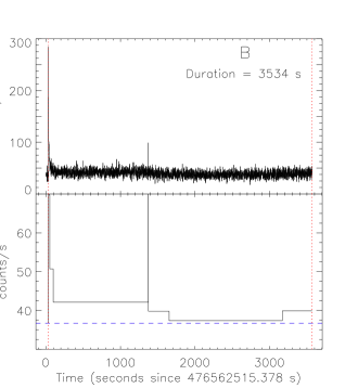
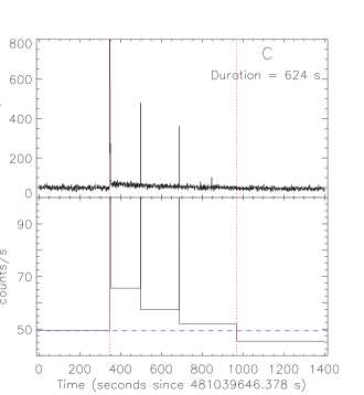
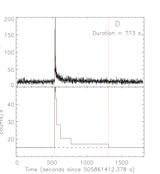
Figure 2.— Top panel: 2$-$20 keV light curves of the four events with 1 s resolution. The four events are identified here with labels A$-$D and indicated in each panel. Bottom panel: Bayesian block representation of the light curve. The blue dashed line represents the background level. Red vertical dotted lines indicate the start and end times of the events. For event B the tail end time is the end of the data (see text).

3. Search for Extended Tails

We implemented a Bayesian blocks based algorithm to identify extended burst tails, which immediately follow the bursts with count rate much lower than that of the burst, but still higher than the count rate of the pre-burst data. The Bayesian block algorithm is a segmentation method in order to detect local variabilities in time series data by separating the data into blocks of statistically significant variations that maximize the likelihood value (Scargle et al., 2013). This method was used to search for weak magnetar bursts by Lin et al. (2013) and resulted in successful detection of the dimmest bursts observed from magnetars.

To optimize the extensive search, we took a two-step approach: a signal-to-noise ratio (S/N) burst identification followed by a Bayesian block tail search, which we describe below. First, we searched for burst candidates in the 0.125 s binned light curves of the source using an S/N criterion with significance 5.5$\sigma$ above background in the 2$-$20 keV energy range. The S/N search identified 878 burst candidates in total. Then, for each of the burst candidates we regenerated the light curves with 1-s resolution, for the interval between 200 s before and 1000 s after the burst time. We then applied the Bayesian block algorithm to the 1 s light curves and obtained the Bayesian block representation of the light curves. Using those, we searched for the increase in the count rate that matches the burst times found by the S/N search. Once found, the beginning of the identified block was taken as the event start time, and the count rate of the preceding block was assigned as the background level. Then, the first decrease in the count rate after the event start time below the assigned background level determines the putative end of the tail. If the algorithm cannot determine the end of the tail within the selected data segment (from T$-$200 to T+1000 s), we extend the post-burst interval by 200 s and perform the search again. For our analysis we run two iterations, and if the algorithm still cannot assign an end to the tail, we conclude that there is no tail associated with that particular burst. We note that the assigned background level can be affected by the existence of data gaps, and in such cases the tail may have been missed in the search. Therefore, to account for such cases, we also artificially elevated the background level to 30$\%$ of the burst candidate’s count rate and performed the search again. The tail end time in such a case was the end of the observation. We eliminated the tail candidates that lasted less than 1 s since extended tails of our interest have much longer durations. Finally, we excluded false detections that are due to known data anomalies.

Based on these criteria, we identified a total of four bursts with extended tails from SGR J1550$-$5418, which we labeled A$-$D in chronological order for convenience in this paper. In Table 1, we provide observational details of these events. Note that our sample includes the two events (events C and D) visually identified and mentioned in Kuiper et al. (2012). In Figure 2, we present the light curves of the bursts with extended tails, as well as their Bayesian block representations. Among these events, the shortest event duration determined by the algorithm is 15 s, and longest duration is 3534 s. For the longest event, the tail end time corresponds to the end of the observation (see Figure 2 top right panel).

Table 2Duration and count rates of bursts and tails in 2$-$25 keV band.

Event	Duration (s)	Counts s-1a
A
Burst	1.83	5573 (5524)
Tail	17.00	102 (53)
B
Burst	0.12	767 (737)
Tail 1	47.07	68 (28)
Tail 2	146.91	47 (7)
C
Burst 1	0.35	18450 (18400)
Burst 2	0.17	2206 (2147)
Burst 3	0.20	1270 (1218)
Tail 1	148.22	74 (19)
Tail 2	187.83	63 (8)
Tail 3	279.80	57 (2)
D
Burst 1	0.30	203 (190)
Burst 2	0.45	340 (329)
Tail 1	113.30	31 (14)
Tail 2	647.40	20 (3)

• The values in parentheses are background-subtracted count rates.
  

4. Spectral Analysis of Tails and Associated Bursts

We investigated spectral properties of the extended tails and the bursts that are associated with these tails in order to uncover their emission properties and compare them with the detected tails from SGR 1900+14 and SGR 1806$-$20. We used HEASOFT v6.16 to perform data extraction. First, we applied standard filtering to the PCA data (Earth occultations, South Atlantic Anomaly passages, electron contamination, etc.). We performed spectral fits using XSPEC software version 12.8.2 (Arnaud, 1996) in energy range 2$-$25 keV, and we used an interstellar H column density of 3.4 $\times$ 10²² cm^-2 which was obtained from Swift data analysis of the source (Lin et al., 2013).

We obtained the background spectra for the bursts from pre-burst data and, when possible, also from post-burst data. For the tails we extracted the background spectra only from the pre-burst data. In all cases we used all layers of operating PCUs and finally grouped the burst and tail spectra such that each spectral bin would contain at least 20 counts (except the burst in event B and burst 1 in event D, which have less counts than other bursts; these are grouped to contain at least 10 counts).

The durations of the four events with tails A, B, C, and D are 15, 3534, 624 and 773 s, respectively, determined based on Bayesian block representation. As mentioned in the previous section, the reason for the long tail duration of event B is that the algorithm could not find a block that goes below the assigned background level before the end of RXTE orbit. We note, however, that the emission after $\sim$200 s is quite weak; in fact, inclusion of data after $\sim$200 s in the spectral analysis did not significantly alter the parameters. Therefore, we limit our investigation by that time.

For each of the four events, we analyzed the burst and tail spectra separately. In the cases of events B, C, and D, the sufficiently long durations of the tails enabled us to investigate the spectral evolutions throughout the tails. To this end, we divided the tails of B and D into two segments, and tail of event C into three segments, separated by the other two bursts in this tail (see Figures 3, 4 and 5), and performed time-resolved spectral analysis. We present the durations and count rates of the burst and tail spectra in Table 2.

For modeling the burst and tail spectra, we employed a set of spectral models that are commonly used for magnetar spectral analysis: single blackbody, double blackbody, optically thin thermal bremsstrahlung, power law, cutoff power law, as well as combinations of these models (see, e.g., Israel et al. (2010); von Kienlin et al. (2012); van der Horst et al. (2012); Lin et al. (2012)). Below, we describe the spectral analysis results of each event. We also present the best-fit spectral parameters determined by the $\chi^{2}$ statistics in Table 3 and spectral evolution of events B, C, and D in Figures 3, 4 and 5. We note that uncertainties are reported at the 1$\sigma$ level throughout the paper.

4.1. Results of Spectral Analysis

4.1.1 Event A

The burst in the beginning of event A was saturated due to high number of burst photons. We therefore excluded the time intervals (a total of $\sim$0.15 s) during which the count rate exceeded 18,000 c s^-1PCU^-1. The burst spectrum is described best with the cutoff power-law model with a photon index of 0.68$\pm$0.08 and cutoff energy 14.24${}^{+1.96}_{-1.57}$ keV ($\chi^{2}_{red}$ = 1.14 with 49 degrees of freedom (dof)). We found that the tail of this event is fitted with a power-law model the best: index of 1.37${}^{+0.10}_{-0.11}$ ($\chi^{2}_{red}$ = 0.84 with 34 dof). The 2$-$25 keV unabsorbed fluxes of the burst and the tail are $>$9.87$\pm$0.12$\times 10^{-8}$ and 9.23$\pm 0.44\times 10^{-10}$ erg cm^-2 s^-1, respectively. The corresponding energies, assuming isotropic emission and the source distance of 5 kpc (Tiengo et al., 2010) are $>$5.39$\times$10³⁸ erg and 4.69$\times$10³⁷ erg for the burst and the tail, respectively. Note that the burst energy is a lower bound since the detector was saturated, and its true energy content was higher than our estimate.

4.1.2 Event B

The burst in event B can be fitted with a single-blackbody model with a temperature of 4.86${}^{+1.06}_{-0.75}$ keV ($\chi^{2}_{red}$ = 0.43 with 6 dof). The time-integrated spectrum of the tail of this event is also best fitted with a blackbody model of kT = 2.22${}^{+0.22}_{-0.19}$ keV ($\chi^{2}_{red}$ = 0.98 with 53 dof). Note that the power-law model for this time-integrated tail yields a similar fit statistics: $\chi^{2}_{red}$ of 1.01 with an index of 1.51$\pm$0.18. We also analyzed the spectra of each segment of the tail and found that both segments are described well with a blackbody model of changing temperature of 3.01${}^{+0.20}_{-0.18}$ and 1.73${}^{+0.22}_{-0.19}$ keV (see Figure 3). The corresponding radii of the blackbody emitting region are 0.25${}^{+0.12}_{-0.11}$ km and 0.36${}^{+0.27}_{-0.22}$ km, respectively (given d = 5 kpc).

4.1.3 Event C

Event C contains three bursts, one in the beginning of the event, the second one $\sim$150 s after the first burst, and the last one separated by $\sim$190 s from the second burst (see Figure 4). The first burst has also saturated the detector due to a high number of incoming burst photons, thus, we excluded the saturated portion of the burst (a total of $\sim$0.18 s), applying the same count rate criterion used for the event A. For this burst, a combination of blackbody and power-law models provided the best fit ($\chi^{2}_{red}$ = 1.24 with 52 dof); the blackbody temperature is 15.46${}^{+4.37}_{-2.58}$ keV and power-law index is 2.01$\pm 0.14$. This corresponds to a blackbody radius of 0.64${}^{+0.45}_{-0.40}$ km. The slightly large $\chi^{2}_{red}$ obtained in this best fit was actually due to the data around 14 keV. Excluding the energy range of 11$-$16 keV from the spectral analysis improves the fit statistics. We will investigate this burst in detail in Şaşmaz Muş, S. et al. (2015, in preparation). Second and third bursts can be fitted well with a power-law model with photon indices 1.43$\pm$0.11 ($\chi^{2}_{red}$ = 1.01 with 13 dof) and 1.79$\pm 0.16$ ($\chi^{2}_{red}$ = 1.00 with 8 dof), respectively. As for the tail, a blackbody model fits the time-integrated tail spectrum very well ($\chi^{2}_{red}$ = 1.18 with 54 dof). The blackbody temperature is 2.12${}^{+0.11}_{-0.10}$ keV, and corresponding radius is 0.24${}^{+0.11}_{-0.10}$ km. The three segments of this tail can also be fitted with the blackbody model, resulting in temperatures of 2.37$\pm 0.11$, 2.17${}^{+0.16}_{-0.15}$ and 1.69${}^{+0.20}_{-0.18}$ keV, respectively (see Figure 4). These correspond to blackbody emitting region radii of 0.29${}^{+0.12}_{-0.11}$, 0.24${}^{+0.13}_{-0.11}$ and 0.25${}^{+0.19}_{-0.15}$ km.

4.1.4 Event D

At the onset of event D, there are two bursts separated by $\sim$11 s. The first burst is best fitted with a single blackbody with a temperature of 5.13${}^{+1.50}_{-0.94}$ keV but still resulted in large $\chi^{2}$ ($\chi^{2}_{red}$ = 1.56 with 4 dof). Further investigation of this burst revealed a possible spectral feature around 14 keV. Similar spectral features around the same energy have been observed in other magnetars (Gavriil et al., 2002; Woods et al., 2005; Gavriil et al., 2006; An et al., 2014). Inclusion of a Gaussian line improves the fit statistics significantly, but energetics are comparable with or without the Gaussian line. This will also be investigated in detail in Şaşmaz Muş, S. et al. (2015, in preparation). The second burst of this event is fitted with a single blackbody with kT = 7.53${}^{+2.39}_{-1.36}$ keV ($\chi^{2}_{red}$ = 0.34 with 5 dof). The time-integrated tail spectrum is also fitted well with a blackbody model with temperature 2.59${}^{+0.13}_{-0.12}$ keV ($\chi^{2}_{red}$ = 0.91 with 53 dof). The corresponding blackbody radius is calculated as 0.18${}^{+0.08}_{-0.07}$ km. Similar to the other events, we found that the tail can be modeled with a blackbody of decreasing temperature, 3.23${}^{+0.14}_{-0.13}$ keV in the first and 2.20${}^{+0.21}_{-0.18}$ keV in the second segment (see Figure 5). The corresponding blackbody radii are 0.22$\pm 0.08$ and 0.19${}^{+0.12}_{-0.10}$ km, respectively.

Table 3Best-fit Spectral Parameters (2$-$25 keV) for the Bursts and the Tails

Event	Modela	kT	Index	BB Radius	Flux (erg cm-2 s-1)	Isotropic Energy (erg)		$\chi^{2}_{red}$(dof)c
		(keV)		(km)	(2$-$25 keV) Unabsorbed	(2$-$10 keV)	(2$-$25 keV)
A
Burst	Cutoff PLb	$-$	0.68$\pm$0.08	$-$	9.87$\pm 0.12\times 10^{-8}$	2.43$\pm 0.03\times 10^{38}$	5.40$\pm 0.07\times 10^{38}$	1.14(49)
Tail	PL	$-$	1.37${}^{+0.10}_{-0.11}$	$-$	9.23$\pm 0.44\times 10^{-10}$	2.11$\pm 0.16\times 10^{37}$	4.69${}^{+0.23}_{-0.22}\times 10^{37}$	0.84(34)
B
Burst	BB	4.86${}^{+1.06}_{-0.75}$	$-$	0.67${}^{+0.52}_{-0.43}$	8.39${}^{+1.28}_{-1.23}\times 10^{-9}$	7.42${}^{+1.25}_{-1.23}\times 10^{35}$	3.01${}^{+0.46}_{-0.44}\times 10^{36}$	0.43(6)
Tail 1+2	BB	2.22${}^{+0.22}_{-0.19}$	$-$	0.28${}^{+0.22}_{-0.18}$	8.06${}^{+0.78}_{-0.75}\times 10^{-11}$	3.17$\pm 0.31\times 10^{37}$	4.68${}^{+0.46}_{-0.44}\times 10^{37}$	0.98(53)
Tail 1	BB	3.01${}^{+0.20}_{-0.18}$	$-$	0.25${}^{+0.12}_{-0.11}$	2.14${}^{+0.15}_{-0.14}\times 10^{-10}$	$-$	$-$	0.91(98)
Tail 2	BB	1.73${}^{+0.22}_{-0.19}$	$-$	0.36${}^{+0.27}_{-0.22}$	4.71${}^{+0.65}_{-0.64}\times 10^{-11}$	$-$	$-$	0.91(98)
C
Burst 1	BB+PL	15.46${}^{+4.37}_{-2.58}$	2.01$\pm$0.14	0.64${}^{+0.45}_{-0.40}$	1.88${}^{+0.06}_{-0.05}\times 10^{-7}$	6.12$\pm 0.16\times 10^{37}$	1.97${}^{+0.07}_{-0.06}\times 10^{38}$	1.24(52)
Burst 2	PL	$-$	1.43$\pm$0.11	$-$	1.89$\pm 0.11\times 10^{-8}$	4.50$\pm 0.33\times 10^{36}$	9.61${}^{+0.55}_{-0.54}\times 10^{36}$	1.01(13)
Burst 3	PL	$-$	1.79$\pm$0.16	$-$	1.08$\pm 0.07\times 10^{-8}$	3.70${}^{+0.39}_{-0.37}\times 10^{36}$	6.45$\pm 0.43\times 10^{36}$	1.00(8)
Tail 1+2+3	BB	2.12${}^{+0.11}_{-0.10}$	$-$	0.24${}^{+0.11}_{-0.10}$	5.06${}^{+0.28}_{-0.27}\times 10^{-11}$	6.60$\pm 0.35\times 10^{37}$	9.32${}^{+0.51}_{-0.50}\times 10^{37}$	1.18(54)
Tail 1	BB	2.37$\pm$0.11	$-$	0.29${}^{+0.12}_{-0.11}$	1.12${}^{+0.06}_{-0.05}\times 10^{-10}$	$-$	$-$	1.18(162)
Tail 2	BB	2.17${}^{+0.16}_{-0.15}$	$-$	0.24${}^{+0.13}_{-0.11}$	5.18${}^{+0.42}_{-0.41}\times 10^{-11}$	$-$	$-$	1.18(162)
Tail 3	BB	1.69${}^{+0.20}_{-0.18}$	$-$	0.25${}^{+0.19}_{-0.15}$	2.07${}^{+0.30}_{-0.29}\times 10^{-11}$	$-$	$-$	1.18(162)
D
Burst 1	BB	5.13${}^{+1.50}_{-0.94}$	$-$	0.43${}^{+0.37}_{-0.30}$	4.14 ${}^{+0.80}_{-0.77}\times 10^{-9}$	8.53$\pm 1.80\times 10^{35}$	3.71${}^{+0.72}_{-0.69}\times 10^{36}$	1.56(4)
Burst 2	BB	7.53${}^{+2.39}_{-1.36}$	$-$	0.39${}^{+0.30}_{-0.26}$	9.63${}^{+0.94}_{-0.98}\times 10^{-9}$	1.96${}^{+0.36}_{-0.34}\times 10^{36}$	1.30$\pm 0.13\times 10^{37}$	0.34(5)
Tail 1+2	BB	2.59${}^{+0.13}_{-0.12}$	$-$	0.18${}^{+0.08}_{-0.07}$	6.03${}^{+0.32}_{-0.31}\times 10^{-11}$	7.83$\pm 0.42\times 10^{37}$	1.37$\pm 0.07\times 10^{38}$	0.91(53)
Tail 1	BB	3.23${}^{+0.14}_{-0.13}$	$-$	0.22$\pm$0.08	2.22$\pm 0.11\times 10^{-10}$	$-$	$-$	1.12(103)
Tail 2	BB	2.20${}^{+0.21}_{-0.18}$	$-$	0.19${}^{+0.12}_{-0.10}$	3.56${}^{+0.36}_{-0.35}\times 10^{-11}$	$-$	$-$	1.12(103)

• PL: power-law model; BB: blackbody model.

• Cutoff energy of this model is 14.24${}^{+1.96}_{-1.57}$ keV.

• We present the simultaneous fit results for the tail segments.

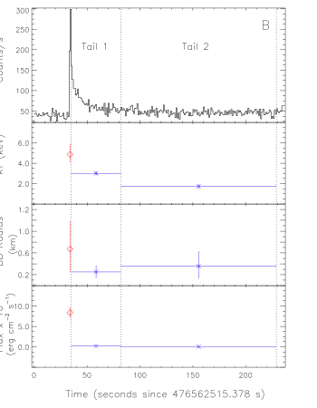
Figure 3.— Spectral parameters of the burst and tail of event B. Top panel: 1 s binned light curve of the event. Dotted vertical lines indicate the time intervals of tail segments. Second panel: blackbody temperature of the burst (red diamond) and tail segments (blue crosses). Third panel: blackbody radii of the burst and tail segments. Bottom panel: unabsorbed fluxes of the burst and tail segments.

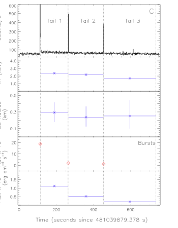
Figure 4.— Spectral parameters of the bursts and tail of event C. Dotted vertical lines indicate the time intervals of tail segments. Top panel: 1 s binned light curve of the event. Second panel: blackbody temperature of the tail segments. Third panel: blackbody radii of the tail segments. Fourth panel: unabsorbed fluxes of the bursts. Bottom panel: unabsorbed fluxes of the tail segments.

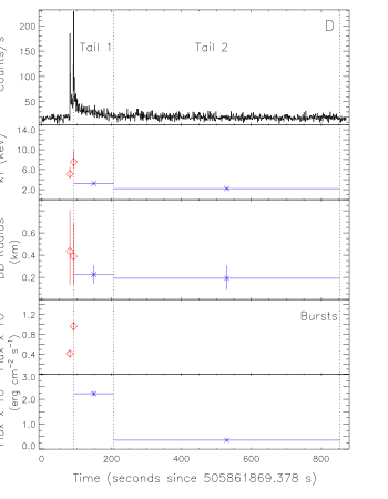
Figure 5.— Spectral parameters of the bursts and tail of event D. Dotted vertical lines indicate the time intervals of tail segments. Top panel: 1 s binned light curve of the event. Second panel: blackbody temperature of the bursts (red diamonds) and tail segments (blue crosses). Third panel: blackbody radii of the bursts and tail segments. Fourth panel: unabsorbed fluxes of the bursts. Bottom panel: unabsorbed fluxes of tail segments.

5. Temporal Analysis

5.1. Phases of Bursts

To investigate whether bursts that exhibit extended tails have any dependence on the spin phase of the neutron star, we have calculated the corresponding phases of the four particular bursts studied here. For this purpose, we used contemporaneous phase-connected spin ephemerides of Dib et al. (2012) for the events A and B, and spin ephemerides or frequencies provided by Kuiper et al. (2012) for the remaining two events. We find that the energetic burst of event A starts at the spin phase, $\phi$ of 0.25, which is the beginning of the peak plateau of the pulse profile (see Figure 6), continues throughout the pulse peak, and declines rapidly after $\phi$ of 0.75, which is the end of the peak plateau. Event B spans the spin phase interval of 0.60 to 0.64. Event C starts at $\phi$ = 0.11, which is the rising part of the pulse profile, and ends somewhere during the peak of the persistent emission. Finally, event D has two spikes separated by 11 s: the first one spans between $\phi$ of 0.91 and 0.95, which is within the minimum phase of the pulse profile, and the second one spans between $\phi$ = 0.10 and 0.22, which is again during the rising portion of the pulse profile.

Figure 6.— Top panel: light curve and pulse profile of the tail detected in event A. Black bars in the pulse profile indicate the phase interval of the other events. D₁ and D₂ denote the two bursts observed in event D.

Figure 7.— Variation of rms fractional amplitude during the tail of event D. The rms fractional amplitudes were calculated at each 50 s time bin during the tail. The dotted vertical line represents the separation between the tail segments considered for the spectral analysis.

5.2. Dependence of Pulse Amplitude on Burst Ignition

Energetic bursts preceding extended tails may induce observable changes in the pulse properties of the neutron star. In order to investigate this for SGR J1550$-$5418, we compared the pulse amplitudes prior to the onset of each of the four events and of those during the tails following the bursts. We created the phase-folded light curves in the 2$-$20 keV energy range considering only PCU 2 for the entire tail and the pre-burst emission of each of the four bursts using the spin ephemerides provided by Dib et al. (2012) and Kuiper et al. (2012) accordingly. We modeled the folded profiles using a sinusoidal model with a harmonic and computed the rms fractional amplitude from the profiles. For event A, the fractional rms amplitude before the burst and during the tail were 1.58$\pm$0.6$\%$ and 17.66$\pm$2.73$\%$, respectively. For event B the pre-burst emission available in the same RXTE orbit was very short, and we estimated the pre-burst pulsation using the data taken during the previous orbit. For this burst, we find that the pulsation amplitudes during pre-burst and tail were 2.32$\pm$1.15$\%$ and 13.68$\pm$2.38$\%$, respectively. For event C, we obtained the pulse amplitude before the burst as 6.51$\pm$2.50$\%$ and in the tail it became 5.07$\pm$1.39$\%$. For the final event D, the amplitudes in the pre-burst emission and the tail were 8.16$\pm$2.25$\%$ and 12.20$\pm$1.75$\%$, respectively.

It was shown for SGR 1900+14 that the pulse fraction increases immediately after the burst and varies with time in the tail of the burst (Lenters et al., 2003). In order to check whether the rms amplitude of pulsation varies during the tail itself for SGR J1550$-$5418, we considered smaller time segments during the tail of all the bursts except the first one and computed the phase-folded profile and rms fractional amplitudes in each of the short time segments. For event D, the rms amplitude is significantly high ($\sim$$0.25$) at the very beginning of the tail just following the burst and then quickly decreases (see Figure 7). The high rms amplitude in the first 50 s of the tail complies with the significant detection of high-power pulsation by Kuiper et al. (2012) in the first 52 s since the onset of that particular burst. After the first 100 s, the fractional rms amplitude value and its variation are consistent with those observed for the pre-burst emission. For event B the average rms amplitude showed a marginal increase during the early episodes of the tail compared to its pre-burst emission, though the increase was not as significant as in the case of event D. For event C, the rms fractional amplitude of pulsation did not vary significantly, remaining generally consistent with the variation of pulse amplitude during the pre-burst emission. To give a measure of the variation of the amplitude of pulsation, we quote the mean and standard deviation of the pulse amplitudes calculated over the finer time segments. The average fractional rms amplitudes during pre-burst and the entire duration of tails for the three events are: 6.24$\pm$4.04$\%$ and 16.68$\pm$1.26$\%$ for event B, 7.93$\pm$4.03$\%$ and 6.90$\pm$3.39$\%$ for event C, and 9.64$\pm$2.80$\%$ and 13.25$\pm$6.32$\%$ for event D. Note that the errors are calculated from the deviations of amplitudes over the short time segments, over which the pulsed signal and fractional rms amplitude could only be poorly constrained.

5.3. Search for QPOs in the Tails of Bursts

We investigated the power spectra during the tails of the four events to search for quasi-periodic oscillations (QPOs) that have been first observed from SGR 1806$-$20 and SGR 1900+14 among magnetars (Israel et al., 2005; Strohmayer & Watts, 2005; Watts & Strohmayer, 2006). For this purpose, we computed the Leahy-normalized power spectra over each 1 s segment during the tail in the energy ranges 2$-$10 and 10$-$30 keV. For QPO detection, we chose a threshold of 3$\sigma$ significance level, considering the number of trials as the number of frequency bins and the number of power spectra searched. Using our criterion, we did not detect any significant QPO features in the individual or averaged power spectra during the burst tails, and the power spectra were consistent with Poisson noise. To further quantify the temporal behavior of the burst tails, we calculated the total noise rms power over the energy bands 2$-$10 and 10$-$30 keV. We divided the burst tails in 15 temporal segments and averaged over them to get the resultant power spectra in each band. We obtained the total rms noise in the 10$-$1020 Hz interval for the two energy bands for event A as 51.09$\%$ and 51.05$\%$, respectively; for event B as 53.28$\%$ and 53.11$\%$, respectively; for event C as 54.24$\%$ and 53.24$\%$, respectively; and finally for event D as 51.96$\%$ and 51.46$\%$, respectively. We also computed the confidence level and corresponding chance occurrence probability of the highest power detected in the power spectrum of each tail, again in the two energy bands. As we present in Table 4, there is no indication of periodic or quasi-periodic processes in the tail of these events.

Table 4Significance levels of the maximum power observed in the power spectra in the 10$-$1020 Hz frequency range.

Event	Total rms	Chance	Number of	Confidence	Significance
	Noise Power	Probability	Trials	Level ($\%$)	($\sigma$)
			Energy Range 2$-$10 keV
A	51.09	1.49$\times 10^{-3}$	1144	18.19	0.23
B	53.28	1.01$\times 10^{-5}$	13061	87.65	1.54
C	54.24	9.44$\times 10^{-5}$	38924	2.54	0.03
D	51.96	7.64$\times 10^{-7}$	51220	96.16	2.07
			Energy Range 10$-$30 keV
A	51.05	3.58$\times 10^{-4}$	1144	66.38	0.96
B	53.11	5.74$\times 10^{-5}$	13061	47.26	0.63
C	53.24	2.91$\times 10^{-5}$	38924	32.21	0.41
D	51.46	1.98$\times 10^{-5}$	51220	36.27	0.47

6. Discussion

We have searched for extended burst tails using the Bayesian blocks technique in a large collection of RXTE data of SGR J1550$-$5418. We identified four events with durations of 15, 3534, 624, and 773 s, and we have studied spectral and temporal properties of these four events. We compare below general properties of these events with one another, as well as those of extended burst tails detected from other magnetars, namely, SGR 1900+14 and SGR 1806$-$20.

The tail of event A has a much shorter duration ($\sim$13 s). Moreover, unlike events B, C and D, its X-ray spectrum has non-thermal character; it is described the best with a power-law model of index 1.37, resembling the SGR burst spectral shape in the RXTE/PCA passband. The other three burst tails have thermal spectra, described with a blackbody model, at temperatures around 2$-$3 keV, and more importantly showing a clear trend of declining blackbody temperature over the course of the tail. According to the magnetar model, the repeated bursts from SGR sources are likely due to fracturing of the solid neutron star crust by magnetic stress (Thompson & Duncan, 1995) or magnetic reconnection (Lyutikov, 2003). In either case, energetic electron$-$positron pair plasma would be induced into the magnetosphere which would be observed as energetic bursts. Note the important fact that event A was detected on 2009 January 22, that is the day SGR J1550$-$5418 was most burst active, and many energetic and relatively long bursts were also detected (see Mereghetti et al. (2009), Savchenko et al. (2010)). Therefore, event A is probably an exceptionally long burst, and the identified tail is most likely the continued emission of this prolonged event.

Extended burst tails were also seen from other magnetars: two from SGR 1900+14, soon after its giant flare in 1998 August and intermediate flare in 2001 April (Ibrahim et al., 2001; Lenters et al., 2003), and two from SGR 1806$-$20 during the 2003$-$2004 burst-active episode prior to its giant flare in 2004 December (Göǧüş et al., 2011). Energies of the bursts leading to extended tails in SGR 1900+14 were at the highest of the scale for typical magnetar bursts. On the other hand, preceding bursts of SGR 1806$-$20 tails were not the highest-energy ones: there were a lot of other energetic bursts that were not followed by tails. Similarly, we found that the energy of the tail triggering burst in SGR J1550$-$5418 could be as low as 3.01$\times 10^{36}$ erg, and there were a lot of more energetic bursts (Mereghetti et al., 2009; van der Horst et al., 2012). The extended tail phenomenon is, therefore, a special case in magnetar bursts; there should be a minimum energy injection to ignite a tail, but not all bursts that are more energetic than the threshold would lead to extended tails. Besides, unlike the other magnetars, in the case of SGR J1550$-$5418 the ratios of total energy contained in the tails and in the bursts seem to vary from event to event. Hence, the question of what ignites extended tails cannot be answered simply with the energetics of the main burst, as already pointed out by Göǧüş et al. (2011).

An important common spectral property of all extended tails observed now from three sources is that they all exhibit thermal spectra and the temperatures decline, that is, cooling throughout the tail. The spectral cooling behavior in SGR J1550$-$5418 is not as significant as in the cases of SGR 1900+14 and SGR 1806$-$20 tails, but still evident. The corresponding blackbody emitting area of SGR J1550$-$5418 tails remains fairly constant around 0.2$-$0.3 km for events B, C, and D. Similar to the earlier tails detected, SGR J1550$-$5418 extended tails are also exhibiting the cooling of a heated portion of the neutron star crust. Given the energetics argument above and the spectral nature of tails, we suggest that the source of heating is the bombardment of the neutron star surface with returning pairs in the trapped fireball (Thompson & Duncan, 1995), which could not efficiently radiate away. Therefore, the consequential cause of the generation of extended tails would depend on how efficiently the trapped plasma in the magnetosphere radiates away.

As far as the temporal investigations of the extended tails are concerned, we do not find any phase dependence of leading bursts, and also any evidence of QPOs in the high-frequency domain, which are observed from the giant flares of SGR 1900+14 and SGR 1806$-$20, and are attributed to torsional oscillations of the neutron star crust (Israel et al., 2005; Strohmayer & Watts, 2005; Watts & Strohmayer, 2006). Apart from other causes, the QPO phenomenon likely requires a much higher burst energetic threshold than that of extended tails to excite torsional modes. Interestingly, we find a significant pulsed amplitude increase in the very early portion of event D, which has one of the least burst energetics. This burst energy argument conditionally strengthens our hypothesis of surface heating with returning pairs because as more energy is imparted back to the system, the energy content of radiated portion would naturally be less.

References

- An et al. (2014) An, H., Kaspi, V. M., Beloborodov, A. M., et al. 2014, ApJ, 790, 60
- Arnaud (1996) Arnaud, K. A. 1996, Astronomical Data Analysis Software and Systems V, 101, 17
- Bernardini et al. (2011) Bernardini, F., Israel, G. L., Stella, L., et al. 2011, A&A, 529, AA19
- Camilo et al. (2007) Camilo, F., Ransom, S. M., Halpern, J. P., & Reynolds, J. 2007, ApJ, 666, L93
- Connaughton & Briggs (2009) Connaughton, V., & Briggs, M. 2009, GCN, 8835, 1
- Dib et al. (2012) Dib, R., Kaspi, V. M., Scholz, P., & Gavriil, F. P. 2012, ApJ, 748, 3
- Duncan & Thompson (1992) Duncan, R. C., & Thompson, C. 1992, ApJ, 392, L9
- Enoto et al. (2012) Enoto, T., Nakagawa, Y. E., Sakamoto, T., & Makishima, K. 2012, MNRAS, 427, 2824
- Enoto et al. (2010) Enoto, T., Nakazawa, K., Makishima, K., et al. 2010, PASJ, 62, 475
- Gavriil et al. (2006) Gavriil, F. P., Kaspi, V. M., & Woods, P. M. 2006, ApJ, 641, 418
- Gavriil et al. (2002) Gavriil, F. P., Kaspi, V. M., & Woods, P. M. 2002, Nature, 419, 142
- Gelfand & Gaensler (2007) Gelfand, J. D., & Gaensler, B. M. 2007, ApJ, 667, 1111
- Göǧüş et al. (2011) Göǧüş, E., Woods, P. M., Kouveliotou, C., et al. 2011, ApJ, 740, 55
- Halpern et al. (2008) Halpern, J. P., Gotthelf, E. V., Reynolds, J., Ransom, S. M., & Camilo, F. 2008, ApJ, 676, 1178
- Ibrahim et al. (2001) Ibrahim, A. I., Strohmayer, T. E., Woods, P. M., et al. 2001, ApJ, 558, 237
- Israel et al. (2010) Israel, G. L., Esposito, P., Rea, N., et al. 2010, MNRAS, 408, 1387
- Israel et al. (2005) Israel, G. L., Belloni, T., Stella, L., et al. 2005, ApJ, 628, L53
- Jahoda et al. (2006) Jahoda, K., Markwardt, C. B., Radeva, Y., Rots, A. H., Stark, M. J., Swank, J. H., Strohmayer, T. E., & Zhang, W. 2006, ApJS, 163, 401
- Kaneko et al. (2010) Kaneko, Y., Göǧüş, E., Kouveliotou, C., et al. 2010, ApJ, 710, 1335
- Krimm et al. (2008) Krimm, H. A., Beardmore, A. P., Gehrels, N., Page, K. L., Palmer, D. M., Starling, R. L. C., & Ukwatta, T. N. 2008, GCN, 8312, 1
- Kouveliotou et al. (2009) Kouveliotou, C., von Kienlin, A., Fishman, G., Connaughton, V., van der Horst, A., & Bhat, N. 2009, GCN, 8915, 1
- Kuiper et al. (2012) Kuiper, L., Hermsen, W., den Hartog, P. R., & Urama, J. O. 2012, ApJ, 748, 133
- Lenters et al. (2003) Lenters, G. T., Woods, P. M., Goupell, J. E., et al. 2003, ApJ, 587, 761
- Lin et al. (2012) Lin, L., Göǧüş, E., Baring, M. G., et al. 2012, ApJ, 756, 54
- Lin et al. (2013) Lin, L., Göǧüş, E., Kaneko, Y., & Kouveliotou, C. 2013, ApJ, 778, 105
- Lyutikov (2003) Lyutikov, M. 2003, MNRAS, 346, 540
- Mereghetti et al. (2009) Mereghetti, S., Götz, D., Weidenspointner, G., et al. 2009, ApJ, 696, L74
- Ng et al. (2011) Ng, C.-Y., Kaspi, V. M., Dib, R., et al. 2011, ApJ, 729, 131
- Olausen & Kaspi (2014) Olausen, S. A., & Kaspi, V. M. 2014, ApJS, 212, 6
- Olausen et al. (2011) Olausen, S. A., Kaspi, V. M., Ng, C.-Y., Zhu, W. W., Dib, R., Gavriil, F. P., & Woods, P. M. 2011, ApJ, 742, 4
- Savchenko et al. (2010) Savchenko, V., Neronov, A., Beckmann, V., Produit, N., & Walter, R. 2010, A&A, 510, A77
- Scargle et al. (2013) Scargle, J. D., Norris, J. P., Jackson, B., & Chiang, J. 2013, ApJ, 764, 167
- Scholz & Kaspi (2011) Scholz, P., & Kaspi, V. M. 2011, ApJ, 739, 94
- Strohmayer & Watts (2005) Strohmayer, T. E., & Watts, A. L. 2005, ApJ, 632, L111
- Tanaka et al. (2010) Tanaka, Y. T., Raulin, J.-P., Bertoni, F. C. P., et al. 2010, ApJ, 721, L24
- Tiengo et al. (2010) Tiengo, A., Vianello, G., Esposito, P., et al. 2010, ApJ, 710, 227
- Thompson & Duncan (1995) Thompson, C., & Duncan, R. C. 1995, MNRAS, 275, 255
- van der Horst et al. (2012) van der Horst, A. J., Kouveliotou, C., Gorgone, N. M., et al. 2012, ApJ, 749, 122
- von Kienlin et al. (2012) von Kienlin, A., Gruber, D., Kouveliotou, C., et al. 2012, ApJ, 755, 150
- von Kienlin & Connaughton (2009) von Kienlin, A., & Connaughton, V. 2009, GCN, 8838, 1
- Watts & Strohmayer (2006) Watts, A. L., & Strohmayer, T. E. 2006, ApJ, 637, L117
- Woods et al. (2005) Woods, P. M., Kouveliotou, C., Gavriil, F. P., et al. 2005, ApJ, 629, 985