Emergent collective chemotaxis without single-cell gradient sensing

Abstract

Many eukaryotic cells chemotax, sensing and following chemical gradients. However, experiments have shown that even under conditions when single cells cannot chemotax, small clusters may still follow a gradient. This behavior has been observed in neural crest cells, in lymphocytes, and during border cell migration in Drosophila, but its origin remains puzzling. Here, we propose a new mechanism underlying this “collective guidance”, and study a model based on this mechanism both analytically and computationally. Our approach posits that the contact inhibition of locomotion (CIL), where cells polarize away from cell-cell contact, is regulated by the chemoattractant. Individual cells must measure the mean attractant value, but need not measure its gradient, to give rise to directional motility for a cell cluster. We present analytic formulas for how cluster velocity and chemotactic index depend on the number and organization of cells in the cluster. The presence of strong orientation effects provides a simple test for our theory of collective guidance.

Cells often perform chemotaxis, detecting and moving toward increasing concentrations of a chemoattractant, to find nutrients or reach a targeted location. This is a fundamental aspect of biological processes from immune response to development. Many single eukaryotic cells sense gradients by measuring how a chemoattractant varies over their length Levine and Rappel (2013); this is distinct from bacteria that measure chemoattractant over time Segall et al. (1986). In both, single cells are capable of net motion toward higher chemoattractant.

Recent measurements of how neural crest cells respond to the chemoattractant Sdf1 suggest that single neural crest cells cannot chemotax effectively, but small clusters can Theveneau et al. (2010). A more recent report shows that at low gradients, clusters of lymphocytes also chemotax without corresponding single cell directional behavior; at higher gradients clusters actually move in the opposite direction to single cells Malet-Engra et al. (2015). In addition, late border cell migration in the Drosophila egg chamber may occur by a similar mechanism Bianco et al. (2007); Rørth (2007); Inaki et al. (2012); Wang et al. (2010). These experiments strongly suggest that gradient sensing in a cluster of cells may be an emergent property of cell-cell interactions, rather than arising from amplifying a single cell’s biased motion; interestingly, some fish schools also display emergent gradient sensing Berdahl et al. (2013). In fact, these experiments led to a “collective guidance” hypothesis Rørth (2007), in which a cluster of cells where each individual cell has no information about the gradient may nevertheless move directionally. In a sense that will become clear, cell-cell interactions allow for a measurement of the gradient across the entire cluster, as opposed to across a single cell.

In this paper, we develop a quantitative model that embodies the collective guidance hypothesis. Our model is based on modulation of the well-known contact inhibition of locomotion (CIL) interaction Lin et al. (2015); Carmona-Fontaine et al. (2008); Desai et al. (2013), in which cells move away from neighboring cells. We propose that individual cells measure the local signal concentration and adjust their CIL strength accordingly; the cluster moves directionally due to the spatial bias in the cell-cell interaction. We discuss the suitability of this approach for explaining current experiments, and provide experimental criteria to distinguish between chemotaxis via collective guidance and other mechanisms where clusters could gain improvement over single-cell migration Simons (2004); Coburn et al. (2013). These results may have relevance to collective cancer motility Friedl et al. (2012), as recent data suggest that tumor cell clusters are particularly effective metastatic agents Aceto et al. (2014).

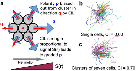
Figure 1: Signal-dependent contact inhibition of locomotion creates directed motion. a, Schematic picture of model and origin of directed motion. Cell polarities are biased away from the cluster toward the direction ${\mathbf{q}}^{i}=\sum_{j\sim i}\hat{{\mathbf{r}}}^{ij}$ by contact inhibition of locomotion (CIL); the strength of this bias is proportional to the local chemoattractant value $S({\mathbf{r}})$, leading to cells being more polarized at higher $S$. See text for details. b, One hundred trajectories of a single cell and c, cluster of seven cells. Trajectories are six persistence times in length (120 min). Scalebar is one cell diameter. The gradient strength is $|\nabla S|=0.025$ in these simulations, with the gradient in the $x$ direction.

We consider a cluster of cells exposed to a chemical gradient $S({\mathbf{r}})$. We use a two-dimensional stochastic particle model to describe cells, giving each cell $i$ a position ${\mathbf{r}}^{i}$ and a polarity ${\mathbf{p}}^{i}$. The cell polarity indicates its direction and propulsion strength: an isolated cell with polarity ${\mathbf{p}}^{i}$ has velocity ${\mathbf{p}}^{i}$. The cell’s motion is overdamped, so the velocity of the cell is ${\mathbf{p}}^{i}$ plus the total physical force other cells exert on it, $\sum_{j\neq i}{\mathbf{F}}^{ij}$. Biochemical interaction between cells alter a cell’s polarity ${\mathbf{p}}^{i}$. Our model is then:

$$\partial_{t}{\mathbf{r}}^{i} ={\mathbf{p}}^{i}+\sum_{j\neq i}{\mathbf{F}}^{ij}$$ (1)

$$\partial_{t}{\mathbf{p}}^{i} =-\frac{1}{\tau}{\mathbf{p}}^{i}+\sigma{\boldsymbol{\xi}}^{i}(t)+\beta^{i}\sum_{j\sim i}\hat{{\mathbf{r}}}^{ij}$$ (2)

where ${\mathbf{F}}^{ij}$ are the intercellular forces of cell-cell adhesion and volume exclusion, and ${\boldsymbol{\xi}}^{i}(t)$ are Gaussian Langevin noises with $\langle\xi^{i}_{\mu}(t)\xi^{j}_{\nu}(t^{\prime})\rangle=2\delta_{\mu\nu}\delta^{ij}\delta(t-t^{\prime})$, where the Greek indices $\mu,\nu$ run over the dimensions $x,y$. The first two terms on the right of Eq. 2 are a standard Ornstein-Uhlenbeck model Selmeczi et al. (2005); Van Kampen (1992): ${\mathbf{p}}^{i}$ relaxes to zero with a timescale $\tau$, but is driven away from zero by the noise $\boldsymbol{\xi}(t)$. This corresponds with a cell that is orientationally persistent over a time of $\tau$.

We have introduced the last term on the right of Eq. 2 to describe contact inhibition of locomotion (CIL). CIL is a well-known property of many cell types in which cells polarize away from cell-cell contact Carmona-Fontaine et al. (2008); Mayor and Carmona-Fontaine (2010); Camley et al. (2014); Abercrombie (1979); Desai et al. (2013). We model CIL by biasing ${\mathbf{p}}^{i}$ away from nearby cells, toward ${\mathbf{q}}^{i}=\sum_{j\sim i}\hat{{\mathbf{r}}}^{ij}$, where $\hat{{\mathbf{r}}}^{ij}=({\mathbf{r}}^{i}-{\mathbf{r}}^{j})/|{\mathbf{r}}^{i}-{\mathbf{r}}^{j}|$ is the unit vector pointing from cell $j$ to cell $i$ and the sum over $j\sim i$ indicates the sum over the neighbors of $i$ (those cells within a distance $D_{0}=1.2$ cell diameters). While this is motivated by CIL in neural crest, it is also a natural minimal model under the assumption that cells know nothing about their neighbors other than their direction $\hat{{\mathbf{r}}}^{ij}$. For cells along the cluster edge, the CIL bias ${\mathbf{q}}^{i}$ points outward from the cluster, but for interior cells ${\mathbf{q}}^{i}$ is smaller or zero (Fig. 1a). This is consistent with experimental observations that edge cells have a strong outward polarity, while interior cells have weaker protrusions Theveneau et al. (2010).

Chemotaxis arises in our model if the chemoattractant $S({\mathbf{r}})$ changes a cell’s susceptibility to CIL, $\beta^{i}$, $\beta^{i}=\bar{\beta}S({\mathbf{r}}^{i})$. This models the result of Theveneau et al. (2010) that the chemoattractant Sdf1 stabilizes protrusions induced by CIL Theveneau et al. (2010). We also assume that the cell’s chemotactic receptors are not close to saturation - i.e. the response is perfectly linear. If CIL is present even in the absence of chemoattractant ($S=0$), as in neural crest Theveneau et al. (2010), i.e. $\beta^{i}=\beta_{0}+\bar{\beta}S({\mathbf{r}})$, this will not significantly change our analysis. Similar results can also be obtained if all protrusions are stabilized by Sdf1 ($\tau$ regulated by $S$), though with some complications (Appendix, Fig. A1).

Analytic predictions for cluster velocity.–Our model predicts that while single cells do not chemotax, clusters as small as two cells will, consistent with Theveneau et al. (2010). We can analytically predict the mean drift of a cluster of cells obeying Eqs. 1-2:

$$\langle{\mathbf{V}}\rangle_{c}\approx\bar{\beta}\tau\mathcal{M}\cdot\nabla S$$ (3)

where the approximation is true for shallow gradients, $S({\mathbf{r}})\approx S_{0}+{\mathbf{r}}\cdot\nabla S$. $\langle{\cdots}\rangle_{c}$ indicates an average over the fluctuating ${\mathbf{p}}^{i}$ but with a fixed configuration of cells ${\mathbf{r}}^{i}$. The matrix $\mathcal{M}$ only depends on the cells’ configuration,

$$\mathcal{M}_{\mu\nu}=\frac{1}{N}\sum_{i}q^{i}_{\mu}r^{i}_{\nu}$$ (4)

where, as above, ${\mathbf{q}}^{i}=\sum_{j\sim i}\hat{{\mathbf{r}}}^{ij}$. Eq. 3 resembles the equation of motion for an arbitrarily shaped object in a low Reynolds number fluid under a constant force $\bar{\beta}\tau\nabla S$ Kim and Karrila (2013): by analogy, we call $\mathcal{M}$ the “mobility matrix.” There is, however, no fluctuation-dissipation relationship as there would be in equilibrium Han et al. (2006).

To derive Eq. 3, we note that Eq. 1 states that, in our units, the velocity of a single cell is equal to the force on it (i.e. the mobility is one). For a cluster of $N$ cells, the mean velocity of the cluster is $1/N$ times the total force on the cluster. As ${\mathbf{F}}^{ij}=-{\mathbf{F}}^{ji}$, the cluster velocity is ${\mathbf{V}}=N^{-1}\sum_{i}{\mathbf{p}}^{i}$. When the cluster configuration changes slowly over the timescale $\tau$, Eq. 2 can be treated as an Ornstein-Uhlenbeck equation with an effectively time-independent bias from CIL. The mean polarity is then $\langle{\mathbf{p}}^{i}\rangle=\beta^{i}\tau\sum_{j\sim i}\hat{{\mathbf{r}}}^{ij}$, with Gaussian fluctuations away from the mean, $\langle({\mathbf{p}}^{i}_{\mu}-\langle{\mathbf{p}}^{i}_{\mu}\rangle)^{2}\rangle=\sigma^{2}\tau$. The mean cell cluster velocity is

$$\langle{{\mathbf{V}}}\rangle_{c}=\frac{\bar{\beta}\tau}{N}\sum_{i}S({\mathbf{r}}^{i})\sum_{j\sim i}\hat{{\mathbf{r}}}^{ij}$$ (5)

In a constant chemoattractant field, $S=S_{0}$, no net motion is observed, as $\sum_{i}\sum_{j\sim i}\hat{{\mathbf{r}}}^{ij}=0$. For linear or slowly-varying gradients $S({\mathbf{r}})\approx S_{0}+{\mathbf{r}}\cdot\nabla S$, and we get Eq. 3.

Cluster motion and chemotactic efficiency depend on cluster size, shape, and orientation.– Within our model, a cluster’s motion can be highly anisotropic. Consider a pair of cells separated by unit distance along $(\cos\theta,\sin\theta)$. Then by Eq. 4, $\mathcal{M}_{xx}=\frac{1}{2}\cos^{2}\theta$, $\mathcal{M}_{xy}=\mathcal{M}_{yx}=\frac{1}{2}\cos\theta\sin\theta$, $\mathcal{M}_{yy}=\frac{1}{2}\sin^{2}\theta$. If the gradient is in the $x$ direction, then $\langle{V_{x}}\rangle_{c}=\frac{V_{0}}{2}\cos^{2}\theta$ and $\langle{V_{y}}\rangle_{c}=\frac{V_{0}}{2}\cos\theta\sin\theta$, where $V_{0}=\bar{\beta}\tau|\nabla S|$. Cell pairs move toward higher chemoattractant, but their motion is along the pair axis, leading to a transient bias in the $y$ direction before the cell pair reorients due to fluctuations in ${\mathbf{p}}^{i}$ (Fig. 2). We compare our theory for the motility of rigid cell clusters (Eq. 3) with a simulation of Eq. 1-2 with strongly adherent cell pairs with excellent agreement (Fig. 2).

For the simulations in Fig. 2 and throughout the paper, we solve the model equations Eqs. 1-2 numerically using a standard Euler-Maruyama scheme. We choose units such that the equilibrium cell-cell separation (roughly 20 $\mu$m for neural crest Theveneau et al. (2010)) is unity, and the relaxation time $\tau=1$ (we estimate $\tau=20$ minutes in neural crest Theveneau et al. (2010)). Within these units, neural crest cell velocities are on the order of $1$, so we choose $\sigma=1$ – this corresponds to a root mean square speed of an isolated cell being $\langle|{\mathbf{V}}|^{2}\rangle^{1/2}=2^{1/2}\sigma\tau^{1/2}\approx 1.4$ microns/minute. The typical cluster velocity scale is $V_{0}=\bar{\beta}\tau|\nabla S|$, which is 0.5 (0.5 microns/minute in physical units) if $|\nabla S|=0.025$ and $S(0)=1$, corresponding to $\beta^{i}$ changing by 2.5% across a single cell at the origin. Cell-cell forces ${\mathbf{F}}^{ij}$ are chosen to be stiff springs so that clusters are effectively rigid (see Appendix for details).

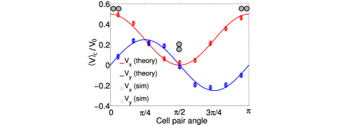
Figure 2: Adherent pairs of cells undergo highly anisotropic chemotaxis. The average chemotactic velocity of a highly adherent cell pair $\langle{V_{x}}\rangle_{c}$ depends strongly on the angle $\theta$ between the cell-cell axis and the chemotactic gradient. Cell pairs also drift perpendicular to the gradient, $\langle{V_{y}}\rangle_{c}\neq 0$. $V_{0}\equiv\bar{\beta}\tau|\nabla S|$ is the velocity scale; $|\nabla S|=0.025$. Simulations are of Eqs. 1-2. We compute $\langle{V_{\mu}}\rangle_{c}$ by tracking the instantaneous angle, then averaging over all velocities within the appropriate angle bin. Error bars here and throughout are one standard deviation of the mean, calculated from a bootstrap. Over $n=13,000$ trajectories of 6$\tau$ (120 minutes) are simulated.

We can also compute $\mathcal{M}$ and hence $\langle V_{x}\rangle$ for larger clusters (Table S1, Appendix, Fig. A2). For a cluster of $Q$ layers of cells surrounding a center cell, $\mathcal{M}_{\mu\nu}=f(Q)\delta_{\mu\nu}$, with $f(Q)=\frac{9Q^{2}+3Q}{2+6Q+6Q^{2}}$. A cluster with $Q$ layers has $N=1+3Q+3Q^{2}$ cells; thus the mean velocity of a $Q$-layer cluster is given by $\langle V_{x}\rangle/V_{0}=\overline{\mathcal{M}}=\frac{3N-\sqrt{12N-3}}{2N}$, where $\overline{\mathcal{M}}=\frac{1}{2}\left(\mathcal{M}_{xx}+\mathcal{M}_{yy}\right)$ is the angular average of $\mathcal{M}$. We predict that $\langle V_{x}\rangle/V_{0}$ first increases with $N$, then slowly saturates to $3/2$. This is confirmed by simulations of the full model (Fig. 3a). We note that $\langle V_{x}\rangle$ is an average over time, and hence orientation (see below, Appendix). We can see why $\langle V_{x}\rangle$ saturates as $N\to\infty$ by considering a large circular cluster of radius $R$. Here, we expect ${\mathbf{q}}^{i}=a\hat{{\mathbf{n}}}$ on the outside edge, where $a$ is a geometric prefactor and $\hat{{\mathbf{n}}}$ is the outward normal, with ${\mathbf{q}}^{i}={\mathbf{0}}$ elsewhere. Then, $\mathcal{M}_{\mu\nu}\sim\frac{a}{\pi R^{2}}\int_{0}^{2\pi}\left(Rd\theta\right)\hat{{\mathbf{n}}}_{\mu}(\theta){\mathbf{r}}_{\nu}=2a\delta_{\mu\nu}$, independent of cluster radius $R$. A related result has been found for circular clusters by Malet-Engra et al. Malet-Engra et al. (2015); we note that they do not consider the behavior of single cells or cluster geometry.

The efficiency of cluster chemotaxis may be measured by chemotactic index (CI), commonly defined as the ratio of distance traveled along the gradient (the $x$ displacement) to total distance traveled Fuller et al. (2010); CI ranges from -1 to 1. We define $\textrm{CI}\equiv\langle V_{x}\rangle/\langle|{\mathbf{V}}|\rangle$, where the average is over both time and trajectories (and hence over orientation). The chemotactic index CI may also be computed analytically, and it depends on the variance of ${\mathbf{V}}$, which is $\langle\left(V_{x}-\langle V_{x}\rangle\right)^{2}\rangle=\langle\left(V_{y}-\langle V_{y}\rangle\right)^{2}\rangle=\sigma^{2}\tau/N$. In our model, CI only depends on the ratio $c$ of mean chemotactic velocity to its standard deviation,

CI $$=\sqrt{2/\pi}c/L_{1/2}(-c^{2}/2)$$

$$c =\frac{\langle V_{x}\rangle}{\sqrt{\langle\left(V_{\mu}-\langle V_{\mu}\rangle\right)^{2}\rangle}}=\frac{\bar{\beta}\tau\overline{\mathcal{M}}|\nabla S|}{\sigma\sqrt{\tau/N}}$$ (6)

where $L_{1/2}$ is a generalized Laguerre polynomial. When mean cluster velocity is much larger than its fluctuations, $c\gg 1$ and $\textrm{CI}\to 1$, but when fluctuations are large, $|c|\ll 1$ and $\textrm{CI}\to 0$ (Appendix, Fig. A3). Together, Eq. 3, Eq. 6 and Table S1 provide an analytic prediction for cluster velocity and CI, with excellent agreement with simulations (Fig. 3). We note that $\langle V_{x}\rangle/V_{0}$ only depends on cluster configuration, where $V_{0}=\bar{\beta}\tau|\nabla S|$, so $\langle V_{x}(N)\rangle/V_{0}$ collapses onto a single curve as the gradient strength is changed (Fig. 3a). By contrast, how CI increases with $N$ depends on $|\nabla S|$ and $\sigma$ (Eq. 6, Fig. 3b).

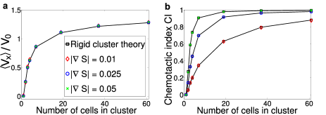
Figure 3: Larger cell clusters chemotax more effectively, but their velocity saturates a, As the number of cells $N$ in a cluster increases, the mean velocity $\langle V_{x}\rangle$ increases with $N$ but then saturates; the mean velocity can be collapsed onto a single curve by rescaling by $V_{0}\equiv\bar{\beta}\tau|\nabla S|$. b, The chemotactic index CI also saturates to its maximum value. Black squares and lines are the orientationally-averaged drift velocity computed for rigid clusters by Eq. 3 and Eq. 6. Colored symbols are full model simulations with strong adhesion. Cell cluster shape may influence $\langle V_{x}\rangle$ (Appendix Fig. A4); our calculations are for the shapes in Table S1. Error bars here are symbol size or smaller; $n\geq 2000$ trajectories of $6\tau$ are used for each point.

In our model, clusters can in principle develop a spontaneous rotation, but in practice this effect is small, and absent for symmetric clusters (see Appendix).

Motion in non-rigid clusters.– While we studied near-rigid clusters above, our results hold qualitatively for clusters that are loosely adherent and may rearrange. Cell rearrangements are common in many collective cell motions Angelini et al. (2010, 2011); Szabó et al. (2010); Vedula et al. (2013), but we note that in Malet-Engra et al. (2015) clusters are more rigid. We choose cell-cell forces ${\mathbf{F}}^{ij}$ to allow clusters to rearrange (see Appendix, Warren (2003)), and simulate Eqs. 1-2. As in rigid clusters, $\langle V_{x}\rangle$ increases and saturates, while CI increases toward unity, though more slowly than a rigid cluster (Fig. 4ab). Clusters may fragment; with increasing $x$, $\beta^{i}$ increases and the cluster breaks up (Fig. 4c). Cluster breakup can limit guidance – if $\bar{\beta}$ is too large, clusters are not stable, and will not chemotax.

In Fig. 4ab, we compute CI and velocity by averaging over all cells, not merely those that are connected. If we track cells ejected from the cluster, they have an apparent $\textrm{CI}>0$, as they are preferentially ejected from the high-$\beta^{i}$ cluster edge (Appendix). Experimental analysis of dissociating clusters may therefore not be straightforward. Anisotropic chemotaxis is present in non-rigid pairs, though lessened because our non-rigid pairs rotate quickly with respect to $\tau$ (Appendix).

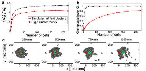
Figure 4: Nonrigid clusters may also chemotax via collective guidance. a, As the number of cells $N$ in a cluster increases, the mean velocity $\langle V_{x}\rangle$ increases with $N$ but then saturates. b, Chemotactic index also approaches unity, but slower than in a rigid cluster. Rigid cluster theory assumes the same cluster geometries as in Fig. 3. Averages in a-b are over $n\geq 20$ trajectories (ranging from $n=20$ for $N=217$ to $n=4000$ for $N=1,2$), over the time $12.5\tau$ to $50\tau$. c, Breakdown of a cluster as it moves up the chemoattractant gradient. X marks the initial cluster center of mass, O the current center. $|\nabla S|=0.1$, $\bar{\beta}=1$ in this simulation.

Distinguishing between potential collective chemotaxis models.–Our model explains how chemotaxis can emerge from interactions of non-chemotaxing cells. However, other possibilities exist for enhancement of chemotaxis in clusters. Coburn et al. showed that in contact-based models, a few chemotactic cells can direct many non-chemotactic ones Coburn et al. (2013). If single cells are weakly chemotactic, cell-cell interactions could amplify this response or average out fluctuations Simons (2004). How can we distinguish these options? In lymphocytes Malet-Engra et al. (2015), the motion of single cells oppositely to the cluster immediately rules out simple averaging or amplification of single cell bias. More generally, the scaling of collective chemotaxis with cluster size does not allow easy discrimination. In Fig. 3, at large $N$, $\langle V_{x}\rangle$ and CI saturate. As an alternate theory, suppose each cell chemotaxes noisily, e.g. ${\mathbf{p}}^{i}=p_{0}\nabla S+\boldsymbol{\Delta}^{i}$, where $\boldsymbol{\Delta}$ are independent zero-mean noises. In this case, $\langle{\mathbf{V}}\rangle=p_{0}\nabla S$ independent of $N$, and $\langle(V_{\mu}-\langle V_{\mu}\rangle)^{2}\rangle\sim 1/N$, as in our large-$N$ asymptotic results and the related circular-cluster theory of Malet-Engra et al. (2015). Instead, we propose that orientation effects in small clusters are a good test of emergent chemotaxis. In particular, studying cell pairs as in Fig. 2 is critical: anisotropic chemotaxis is a generic sign of cluster-level gradient sensing. Even beyond our model, chemotactic drift is anisotropic for almost all mechanisms where single cells do not chemotax, because two cells separated perpendicular to the gradient sense the same concentration. This leads to anisotropic chemotaxis unless cells integrate information over times much larger than the pair’s reorientation time. By contrast, the simple model with single cell chemotaxis above leads to isotropic chemotaxis of pairs.

How well does our model fit current experiments? We find increasing cluster size increases cluster velocity and chemotactic index. This is consistent with Malet-Engra et al. (2015), who see a large increase in taxis from small clusters ($<20$ cells) to large, but not Theveneau et al. (2010), who find that CI is similar between small and large clusters, and note no large variations in velocity. This suggests that the minimal version of collective guidance as developed here can create chemotaxis, but does not fully explain the experiments of Theveneau et al. (2010). There are a number of directions for improvement. More quantitative comparisons could be made by detailed measurement of single-cell statistics Selmeczi et al. (2005); Amselem et al. (2012), leading to nonlinear or anisotropic terms in Eq. 2. Our description of CIL has also assumed, for simplicity, that both cell front and back are inhibitory; other possibilities may alter collective cell motion Camley et al. (2014). We could also add adaptation as in the LEGI model Levchenko and Iglesias (2002); Takeda et al. (2012) to enable clusters to adapt their response to a value independent of the mean chemoattractant concentration. We will treat extensions of this model elsewhere; our focus here is on the simplest possible results.

In summary, we provide a simple, quantitative model that embodies a minimal version of the collective guidance hypothesis Rørth (2007); Theveneau et al. (2010) and provides a plausible initial model for collective chemotaxis when single cells do not chemotax. Our work allows us to make an unambiguous and testable prediction for emergent collective guidance: pairs of cells will develop anisotropic chemotaxis. Although there has been considerable effort devoted to models of collective motility Sepúlveda et al. (2013); Camley and Rappel (2014); Szabo et al. (2006); Li and Sun (2014); Czirók et al. (1996); van Drongelen et al. (2015); Basan et al. (2013); Zimmermann et al. (2014); Szabó et al. (2010); Segerer et al. (2015), ours is the first model of how collective chemotaxis can emerge from single non-gradient-sensing cells via collective guidance and regulation of CIL.

I Appendix

II Cluster chemotaxis when chemoattractant regulates cell persistence $\tau$

Within the main paper, we have assumed that the chemoattractant concentration $S({\mathbf{r}})$ regulates the susceptibility of a cell to contact inhibition of locomotion $\beta^{i}$, with $\beta^{i}=\bar{\beta}S({\mathbf{r}}^{i})$. This models the stabilization of protrusions induced by contact interactions. This is consistent with the results of Theveneau et al. Theveneau et al. (2010), who find that protrusion stabilization is stronger in clusters than in single cells. However, very similar results can be found if we assume that $\beta$ is constant and the signal regulates the time required for the cell’s polarity to relax, i.e. $\tau^{i}=\bar{\tau}S({\mathbf{r}})$. In this case, the mean polarity of a cell is $\langle{\mathbf{p}}^{i}\rangle=\beta\tau^{i}\sum_{j\sim i}\hat{{\mathbf{r}}}^{ij}$ and we find

$$\langle{\mathbf{V}}\rangle\approx\beta\bar{\tau}\mathcal{M}\cdot\nabla S\;\;(\tau\,\textrm{ regulation})$$ (A1)

where the mobility matrix $\mathcal{M}$ is the same as in the main paper, $\mathcal{M}_{\mu\nu}=\frac{1}{N}\sum_{i}r^{i}_{\nu}q^{i}_{\mu}$. However, because $\tau$ varies over space, the fluctuations will also vary: $\langle\left(V_{\mu}-\langle V_{\mu}\rangle\right)^{2}\rangle=\sigma^{2}N^{-2}\sum_{i}\tau^{i}=\sigma^{2}N^{-1}\bar{\tau}\overline{S}$, where $\overline{S}=N^{-1}\sum_{i}S({\mathbf{r}}^{i})$ is the mean signal across the cluster. For this reason, the chemotactic index in the $\tau$-regulation model will depend on $\nabla S/\overline{S}^{1/2}$, and will not be constant over a linear gradient.

In addition, a single cell with a persistence time $\tau$ that depends on the chemoattractant level will undergo biased motion. This is shown in Fig. A1 below. This drift can be made smaller than the CIL-driven cluster drift, as it is independent of $\beta$, while the cluster drift is proportional to $\beta$.

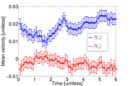
Figure A1: Single cells in a spatially-varying $\tau$ develop a mean drift. The mean $x$ and $y$ velocities for a cell with spatially varying $\tau$ are shown: $\tau=\overline{\tau}\left(S_{0}+|\nabla S|x\right)$, with $\overline{\tau}=1$, $S_{0}=1$, $|\nabla S|=0.025$. Result is average over $n=10^{5}$ iterations, each started at the origin; error bars indicate $\langle\left[V_{\mu}(t)-\langle V_{\mu}(t)\rangle\right]^{2}\rangle^{1/2}/\sqrt{n}$.

III Derivation of the mobility matrices for $Q$-layer oligomers

We can compute the mobility matrix of the $Q$-layer oligomers for arbitrary $Q$. Our mobility matrix is given by Eq. 4 with ${\mathbf{q}}^{i}=\sum_{j\sim i}\hat{{\mathbf{r}}}^{ij}$. To simplify the calculation, we can make a few assumptions. First, we note that $\mathcal{M}_{xx}=\mathcal{M}_{yy}$, but $\mathcal{M}_{xy}=\mathcal{M}_{yx}=0$ for the $Q$-layer oligomer. We only need to calculate $\overline{\mathcal{M}}=\frac{1}{2}\left(\mathcal{M}_{xx}+\mathcal{M}_{yy}\right)$. The only cells $i$ in the sum of Eq. 4 that are nonzero are those around the boundary. $\overline{\mathcal{M}}$ does not depend on orientation, so we can compute the sum $\sum_{i}{\mathbf{r}}^{i}{\mathbf{q}}^{i}$ for one face of the oligomer (Fig. A2), then multiply by six. However, this double-counts the corner cells, so we must weight them by $1/2$. We then find $\overline{\mathcal{M}}=\left[\frac{9}{2}Q^{2}+\frac{3}{2}Q\right]/N(Q)$, where $N(Q)=1+3Q+3Q^{2}$ is the number of cells in the cluster.

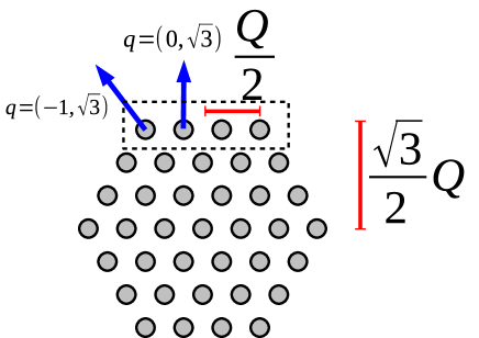
Figure A2: Geometry of $Q$-layer oligomer, illustrated for $Q=3$. The top face is highlighted by a dashed line.

We present the mobility matrices for both $Q$-layer oligomers and other cluster shapes in Table A1.

Shape	$\mathcal{M}$	Angularly averaged $\overline{\mathcal{M}}$
Dimer	$\begin{pmatrix}1/2&0\\ 0&0\end{pmatrix}$	1/4
Trimer	$\begin{pmatrix}1/2&0\\ 0&1/2\end{pmatrix}$	1/2
Tetramer	$\begin{pmatrix}1/2&0\\ 0&3/4\end{pmatrix}$	5/8
Heptamer	$\begin{pmatrix}6/7&0\\ 0&6/7\end{pmatrix}$	6/7
Q-layer oligomer	$\begin{pmatrix}$f(Q)$&0\\ 0&$f(Q)$\end{pmatrix}$	$f(Q)\equiv\frac{9Q^{2}+3Q}{2+6Q+6Q^{2}}$

Table A1: Mobility matrices $\mathcal{M}$ for several cell configurations. For each of the configurations shown, nearest-neighbor cells have unit separation. A $Q$-layer oligomer has $N(Q)=1+3Q+3Q^{2}$ cells. $\mathcal{M}$ is given for the orientation shown in the left column; other orientations may be found by transforming the mobility tensor; $\overline{\mathcal{M}}=\frac{1}{2}\left(\mathcal{M}_{xx}+\mathcal{M}_{yy}\right)$ (see Section IV below).

IV Rotational transformation and averaging of the mobility matrix

We can compute the mobility matrix of a rotated cluster of arbitrary shape from Eq. 4. If we rotate our cluster, which we assume is centered at the origin, by an angle $\theta$, $\left({\mathbf{r}}^{i}\right)^{\prime}=\mathcal{R}(\theta){\mathbf{r}}^{i}$, we find that

$$\mathcal{M}^{\prime}_{\mu\nu}=\mathcal{R}_{\mu\alpha}(\theta)\mathcal{M}_{\alpha\beta}\mathcal{R}_{\nu\beta}(\theta)$$ (A2)

where we have assumed the Einstein summation convention and $\mathcal{R}(\theta)$ is the rotation matrix $\left(\begin{array}[]{cc}\cos\theta&-\sin\theta\\ \sin\theta&\cos\theta\end{array}\right)$. In matrix terms, $\mathcal{M}^{\prime}=\mathcal{R}(\theta)\cdot\mathcal{M}\cdot\left[\mathcal{R}(\theta)\right]^{T}$. If we average over $\theta$, we find

$$\frac{1}{2\pi}\int_{0}^{2\pi}d\theta\mathcal{M}^{\prime}(\theta)=\frac{1}{2}\left(\begin{array}[]{cc}\mathcal{M}_{xx}+\mathcal{M}_{yy}&\mathcal{M}_{xy}-\mathcal{M}_{yx}\\ \mathcal{M}_{yx}-\mathcal{M}_{xy}&\mathcal{M}_{xx}+\mathcal{M}_{yy}\end{array}\right)$$ (A3)

We can show from the definition Eq. 4 that $\mathcal{M}_{\mu\nu}=\mathcal{M}_{\nu\mu}$, so the off-diagonal entries of the averaged matrix are zero, and therefore $\frac{1}{2\pi}\int_{0}^{2\pi}d\theta\mathcal{M}_{\mu\nu}^{\prime}(\theta)=\frac{1}{2}(\mathcal{M}_{xx}+\mathcal{M}_{yy})\delta_{\mu\nu}$. In other words, when averaged over orientation, a cell cluster’s mobility matrix is just the constant $\overline{\mathcal{M}}$ times the identity.

V Computing the chemotactic index

We showed in the main paper that within our model, assuming that the cluster rearrangement is slow with respect to the polarity dynamics and thus each cell’s polarity is given by a biased Ornstein-Uhlenbeck process, the velocity of a rigid cell cluster is

$${\mathbf{V}}=\langle{\mathbf{V}}\rangle+\boldsymbol{\Delta}$$ (A4)

where $\Delta$ is a Gaussian random variable with zero mean and variance $\langle\Delta_{\mu}\Delta_{\nu}\rangle=\Gamma^{2}\delta_{\mu\nu}$. We want to compute the chemotactic index, CI; assuming the gradient is increasing in the $x$ direction, this is

$$\textrm{CI}=\frac{\langle V_{x}\rangle}{\langle|{\mathbf{V}}|\rangle}$$ (A5)

where the average is both over time and over many trajectories. We note that this is a useful definition for us because, in our model, neither $\langle{\mathbf{V}}\rangle$ nor $\Delta$ depend on the absolute value of the chemoattractant $S$. More care must be taken in other cases. To compute CI, we need to compute $\langle|{\mathbf{V}}|\rangle$. $|{\mathbf{V}}|$ is, in our case, given by a Rice distribution, and this moment can be calculated.

$$\langle|{\mathbf{V}}|\rangle =\langle\sqrt{(\langle V_{x}\rangle+\Delta_{x})^{2}(\langle V_{y}\rangle+\Delta_{y})^{2}}\rangle$$ (A6)

$$=\frac{1}{2\pi\Gamma^{2}}\int d\Delta_{x}d\Delta_{y}\sqrt{(\langle V_{x}\rangle+\Delta_{x})^{2}+(\langle V_{y}\rangle+\Delta_{y})^{2}}\exp\left[\frac{-(\Delta_{x}^{2}+\Delta_{y}^{2})}{2\Gamma^{2}}\right]$$ (A7)

$$=\frac{1}{2\pi\Gamma^{2}}\int dV_{x}dV_{y}V\exp\left[-\frac{1}{2\Gamma^{2}}\left\{(V_{x}-\langle V_{x}\rangle)^{2}+(V_{y}-\langle V_{y}\rangle)^{2}\right\}\right]$$ (A8)

where $V=\sqrt{V_{x}^{2}+V_{y}^{2}}$. We now switch to polar coordinates, $V_{x}=V\cos\phi$, $V_{y}=V\sin\phi$, and correspondingly write $\langle V_{x}\rangle=\nu\cos\theta$ and $\langle V_{y}\rangle=\nu\sin\theta$, where $\nu^{2}=\langle V_{x}\rangle^{2}+\langle V_{y}\rangle^{2}$. Thus,

$$\langle|{\mathbf{V}}|\rangle =\frac{1}{2\pi\Gamma^{2}}\int_{0}^{2\pi}d\phi\int_{0}^{\infty}dVV^{2}\exp\left[-\frac{1}{2\Gamma^{2}}\left\{V^{2}+\nu^{2}-2V\nu\cos(\theta-\phi)\right\}\right]$$ (A9)

$$=\frac{1}{\Gamma^{2}}\int_{0}^{\infty}dVV^{2}\exp\left[-\frac{1}{2\Gamma^{2}}\left(V^{2}+\nu^{2}\right)\right]I_{0}\left(V\nu/\Gamma^{2}\right)$$ (A10)

where $I_{0}(x)$ is the modified Bessel function of the first kind. This integral may be evaluated, resulting in

$$\langle|{\mathbf{V}}|\rangle=\Gamma\sqrt{\pi/2}L_{1/2}(-\nu^{2}/2\Gamma^{2})$$ (A11)

where the generalized Laguerre polynomial $L_{1/2}$ is given by

$$L_{1/2}(x)=e^{x/2}\left[(1-x)I_{0}(-x/2)-xI_{1}(-x/2)\right].$$ (A12)

Within our average over trajectories, we are averaging over the orientation of the cluster; thus we expect $\langle V_{y}\rangle$ = 0 for a chemoattractant gradient in the $x$ direction, and $\nu=\langle V_{x}\rangle=\bar{\beta}\tau\overline{\mathcal{M}}\partial_{x}S$. $\Gamma^{2}=\langle\left(V_{x}-\langle V_{x}\rangle\right)^{2}\rangle=\langle\left(V_{y}-\langle V_{y}\rangle\right)^{2}\rangle=\sigma^{2}\tau/N$. This leads to the result stated in the main paper,

CI $$=\sqrt{2/\pi}c/L_{1/2}(-c^{2}/2)$$

$$c =\frac{\langle V_{x}\rangle}{\sqrt{\langle\left(V_{\mu}-\langle V_{\mu}\rangle\right)^{2}\rangle}}=\frac{\bar{\beta}\tau\overline{\mathcal{M}}\partial_{x}S}{\sigma\sqrt{\tau/N}}$$ (A13)

where in our notation, we could also write $c=\nu/\Gamma$. We plot the result of Eq. 6 in Fig. A3 below; we see that $\textrm{CI}\to 1$ as $c\gg 1$ (corresponding to cluster velocities much larger than the noise in cluster velocity) and $\textrm{CI}\to 0$ if $|c|\ll 1$ (cluster velocity much smaller than the noise). We also note that chemotaxis could oppose the direction of the gradient (chemorepulsion) – in this case, $\textrm{CI}(-c)=-\textrm{CI}(c)$.

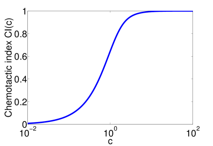
Figure A3: Chemotactic index CI as a function of the parameter $c$.

VI Velocity and CI of irregular clusters

In the main paper, we presented results on the velocity and chemotactic index of $Q$-layer oligomers. Here, we show the velocity and chemotactic index of imperfect clusters. We begin with a $Q$-layer oligomer, and then remove $n$ cells at random from the outer layer; this process is repeated 200 times for each $n$ from 1 to $6Q$ (the number of cells in the outer layer). An example is presented in Fig. A4, with $Q=5$ and $n=5$ cells removed. The mobility matrix is computed for each cluster, and used to compute $\langle V_{x}\rangle$ and CI (Fig. A4). We see that though different configurations can lead to different mean velocities for the same number of cells, the general trend is captured by the results for intact oligomers (dashed line and square symbols in Fig. A4).

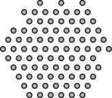
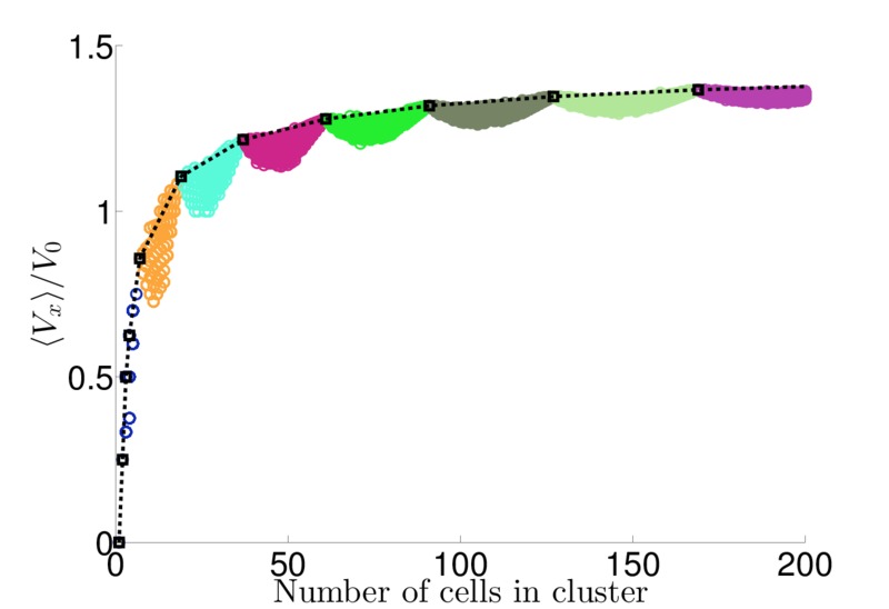
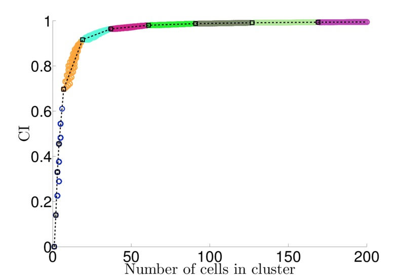
Figure A4: Cluster shape effects, in addition to cell number, can affect velocity and CI. Top: illustration of $Q$-layer oligomer with a few cells removed from the external layer. Bottom: Velocity and chemotactic index for clusters of different shapes. Different colors indicate the size of the base cluster from which cells are removed. Black squares connected by dashed lines show the results for intact oligomers. For the CI plot, we apply our usual parameters and $|\nabla S|=0.025$. All results in this figure are theoretical results for rigid clusters only, not full simulations.

VII Transient rotation of clusters

Though we have primarily focused on the translational motion of the cluster, rotational motion can also occur in our model, both through rotational diffusion and biased motion. We note that transient rotational events are observed in Malet-Engra et al. (2015). Under assumptions similar to our main results, clusters have mean angular velocity $\sim{\mathbf{A}}\cdot\nabla S$, where ${\mathbf{A}}$ depends on cluster geometry. This is again similar to an oddly-shaped particle sedimenting in a low Reynolds number flow Kim and Karrila (2013). However, the symmetric clusters in Table S1 have ${\mathbf{A}}={\mathbf{0}}$ and do not rotate. If ${\mathbf{A}}\neq{\mathbf{0}}$, clusters rotate to a fixed angle to the gradient direction; there is no persistent rotation in a linear gradient (rotational motion may also be suppressed if $\bar{\beta}$ is large). However, in nonlinear gradients, persistent rotation of asymmetric clusters may be induced.

We can analyze potential biases by determining the net “torque” $L_{z}=\sum_{i}\left[\boldsymbol{\delta}{\mathbf{r}}^{i}\times{\mathbf{p}}^{i}\right]_{z}$ applied to the cluster by the cells. This torque is, on average,

$$\langle L_{z}\rangle=\sum_{i}\bar{\beta}\tau S({\mathbf{r}}^{i})\left[\boldsymbol{\delta}{\mathbf{r}}^{i}\times{\mathbf{q}}^{i}\right]_{z}$$ (A14)

where ${\mathbf{q}}^{i}=\sum_{j\sim i}\hat{{\mathbf{r}}}^{ij}$ and $\boldsymbol{\delta}{\mathbf{r}}^{i}={\mathbf{r}}^{i}-{\mathbf{r}}_{\textrm{cm}}$ is the displacement from the cluster center of mass.

What torque is required to cause the cluster to move at a fixed angular velocity? For a cluster moving in a rigid rotation with angular velocity $\Omega$, the cell velocities are ${\mathbf{v}}^{i}=\Omega\left(-\delta r_{y}^{i},\delta r_{x}^{i}\right)$. To achieve this, each cell must have a polarity of ${\mathbf{p}}^{i}=\Omega\left(-\delta r_{y}^{i},\delta r_{x}^{i}\right)$, leading to $L_{z}=\Omega\sum_{i}|\boldsymbol{\delta}{\mathbf{r}}^{i}|^{2}$. The angular velocity is thus related to $L_{z}$ by $\Omega=L_{z}/\sum_{i}|\boldsymbol{\delta}{\mathbf{r}}^{i}|^{2}$. We thus find, for linear gradients, $S=S_{0}+{\mathbf{r}}\cdot\nabla S$,

$$\langle\Omega\rangle=\bar{\beta}\tau{\mathbf{A}}\cdot\nabla S$$ (A15)

where the vector ${\mathbf{A}}$ only depends on the cluster geometry,

$${\mathbf{A}}=\frac{\sum_{i}\boldsymbol{\delta}{\mathbf{r}}^{i}\left[\boldsymbol{\delta}{\mathbf{r}}^{i}\times{\mathbf{q}}^{i}\right]_{z}}{\sum_{i}|\boldsymbol{\delta}{\mathbf{r}}^{i}|^{2}}$$ (A16)

where ${\mathbf{q}}^{i}$ is defined as above. (Note that $\sum_{i}\boldsymbol{\delta}{\mathbf{r}}^{i}\times{\mathbf{q}}^{i}=\sum_{i}{\mathbf{r}}^{i}\times{\mathbf{q}}^{i}=-\sum_{i,j\sim i}\frac{{\mathbf{r}}^{i}\times{\mathbf{r}}^{j}}{|{\mathbf{r}}^{i}-{\mathbf{r}}^{j}|}=0$, allowing us to drop a center of mass term.) For all of the shapes listed in Table A1, ${\mathbf{A}}={\mathbf{0}}$. Cell clusters must lack an inversion symmetry to be rotated by the gradient.

However, even if ${\mathbf{A}}\neq{\mathbf{0}}$, clusters will not persistently rotate. We can see that if we rotate the cell cluster around its center of mass, ${\mathbf{A}}$ must also rotate as a vector. If the gradient is along the $x$ direction, this lets us write $\langle\Omega\rangle=\langle\dot{\theta}\rangle=\bar{\beta}\tau\left[A_{x}(0)\cos\theta-A_{y}(0)\sin\theta\right]$, where ${\mathbf{A}}(0)$ is Eq. A16 calculated for a reference geometry. We see that if ${\mathbf{A}}\neq{\mathbf{0}}$, the cluster will rotate to a stable angle $\theta^{*}$ given by $\tan\theta^{*}=A_{x}(0)/A_{y}(0)$. In a linear gradient, there is no persistent rotation, though in nonlinear gradients, persistent rotation of asymmetric clusters may be induced.

We note that Eq. A15 is not as quantitatively accurate as the corresponding result for translational motion, at least for the parameter set in the main paper; this occurs because a small deviation from the equilibrium polarity $\langle{\mathbf{p}}^{i}\rangle$ can create a relatively large change in torque, which often resists rotation. For instance, if the cluster is rotated by a small angle $\delta$ without a corresponding change in $\langle{\mathbf{p}}^{i}\rangle$, there will be a restoring torque proportional to $\bar{\beta}\tau\delta$. Thus, Eq. A15 will be more accurate for systems where the relaxation time $\tau$ is smaller compared to the rotational timescale of the cluster. For similar reasons, for our rigid cluster parameter set, rotational diffusion can be quite slow (Movie S1).

VIII Nonrigid cluster simulations

In this section, we present additional results on nonrigid clusters. We observe that the cluster anisotropy observed in Fig. 2 of the main paper persists in fluid clusters, but is somewhat weaker (Fig. A5). This occurs because the rotational diffusion of pairs of cells at our nonrigid parameter set is significantly faster than that of the rigid parameter set (compare Movie S1, Movie S2). As the cluster’s polarities $\langle{\mathbf{p}}^{i}\rangle$ are influenced by the cluster orientation over a timescale $\tau$, as diffusion becomes faster with respect to $\tau$, anisotropy decreases. We also note that we would not expect our rigid-cluster results to be precisely accurate even without this effect, as the pair’s separation will fluctuate around its equilibrium value, changing $\mathcal{M}$.

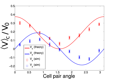
Figure A5: Anisotropy exists but is lower in nonrigid clusters. A pair of cells with our nonrigid cluster parameters has anisotropic chemotaxis, but with a slightly weaker anisotropy. Trajectories here are measured over the time range $6.25\tau$ to $50\tau$; $n=20,200$ trajectories are simulated. Rigid cluster results are computed using a cell-cell spacing of 0.75 to roughly match the separation seen in simulations, so the curves plotted are $0.75\times\frac{1}{2}\cos^{2}\theta$ and $0.75\times\frac{1}{2}\cos\theta\sin\theta$.

We presented in the main paper a figure showing how the cluster velocity and chemotactic index depend on the cluster size (Fig. 4 of the main paper). However, in Fig. 4, we treat all of the cells that were initially in contact as a single cluster, even if they broke apart – thus we are plotting velocity and CI versus the total number of cells in the simulation. An alternate way to compute a curve showing velocity and CI as a function of cluster size would be to look at a simulation in which an initially large cluster breaks into smaller clusters (as seen in Theveneau et al. (2010)), and then track the smaller clusters. Doing this can yield different results, because the history of the smaller clusters matters. In particular, clusters are more likely to break off from the side of the big cluster at higher $S$ (see e.g. Movie S2) – leading to important biases. For instance, we note in Fig. A6a that smaller clusters (which have been ejected) have a larger velocity than large ones, even though isolated small clusters are slower than isolated large clusters. Similarly, we see in Fig. A6b that even isolated cells develop an apparent chemotactic index. This occurs even though single isolated cells in our model have a behavior that is completely independent of the chemotactic signal – if a single cell is isolated for a long enough time, its dynamics will again be unbiased.

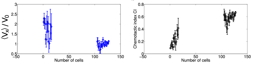
Figure A6: Analyzing clusters in the process of breaking down can lead to apparent single-cell chemotaxis. Tracking clusters as they break off from a larger cluster leads to an increased velocity for smaller clusters, and a non-zero chemotactic index even for single cells. This figure is generated by simulating clusters initially of 127 cells (6-layer oligomers) over a time of $50\tau$ (1000 minutes), and then computing the average velocity and average instantaneous chemotactic index $V_{x}/|{\mathbf{V}}|$ as a function of the number of cells in a given sub-cluster; 200 different trajectories are used. We discard the first 25$\tau$ of the trajectory, so we are focusing on the late cluster breakup stage. Two cells are considered to be in the same cluster if they are within a distance $D_{0}$ of one another (e.g. the force between them is nonzero). We only show points in this figure where we have at least $25\tau$ of trajectory time with clusters of that size totaled over all 200 simulations. Clusters of, e.g. 50 cells are not typically seen, and therefore not shown in this figure.

IX Numerical details of full model simulation

For our simulations, we solve the model equations numerically using a standard Euler-Maruyama scheme. For our rigid cluster simulations, we adapt the cell-cell force from Szabo et al. (2006)

$${\mathbf{F}}^{ij}=\hat{{\mathbf{r}}}^{ij}\left\{\begin{array}[]{lr}v_{r}\left(d^{ij}-1\right),&\;\;d^{ij}<1\\ v_{a}\frac{d^{ij}-1}{D_{0}-1},&\;\;1\leq d^{ij}<D_{0}\\ 0&\;\;d^{ij}>D_{0}\end{array}\right.$$ (A17)

where $d^{ij}=|{\mathbf{r}}^{i}-{\mathbf{r}}^{j}|$. This force is a repulsive spring below the equilibrium separation (which is one in our units, 20 microns in physical units), an attractive spring above it, and vanishes above $D_{0}$. $D_{0}=1.2$ in all of our simulations, and we use $v_{r}=v_{a}=500$. This keeps the clusters very rigid.

For our non-rigid cluster simulations, we adapt the many-body force chosen by Warren to simulate vapor-liquid coexistence Warren (2003),

$${\mathbf{F}}^{ij}=\left[Aw(d^{ij}/D_{0})+B\left(\overline{\rho}^{i}+\overline{\rho}^{j}\right)w(d^{ij})\right]\hat{{\mathbf{r}}}^{ij}$$ (A18)

where $w(r)=(1-r)$ for $r\leq 1$ and $0$ otherwise. The densities are defined by $\overline{\rho}^{i}=\sum_{j}w_{\rho}(d^{ij})$, where the sum is over all cells, including $i$, and $w_{\rho}(r)=\frac{6}{\pi}(1-r)^{2}$ for $r\leq 1$ and $0$ otherwise. The force of Eq. A18 is composed of an attractive force that goes to zero at a separation of $D_{0}$, and a repulsive force that is zero beyond the distance of cell-cell overlap (1 in our units). Both attractive and repulsive forces have a finite value even with cells completely overlapping (“soft cores”). The strength of the repulsive force increases with increasing cell density – this makes the force explicitly dependent on many-body interactions. This force makes developing fluid droplets relatively easy, even with short-range interactions Warren (2003). We use $A=-23.1$ and $B=7.35$ for our non-rigid cluster simulations unless otherwise noted.

We initialize our clusters centered at the origin. For rigid clusters, we start our simulations with the shapes given in Table A1 but rotated to a random angle, and a spacing of the equilibrium spacing (unity) for rigid clusters. For non-rigid clusters, we start with the appropriate $Q$-layer cluster at a random angle, but with a spacing of $0.7$. For non-rigid clusters, we initialize 2-, 3-, and 4-cell clusters by removing the appropriate number of cells randomly from the outer layer of a heptamer. In both cases, we initialize the polarity ${\mathbf{p}}$ to a random value from its distribution (i.e. $\beta^{i}\tau{\mathbf{q}}^{i}$ plus an appropriate noise).

X Table of parameters

Parameter symbol	Name	Value in our units
$\tau$	Persistence time	1
$\sigma$	Characteristic cell speed (OU noise parameter)	1
$\bar{\beta}$	CIL strength	20 for rigid clusters, 1 for nonrigid clusters
$v_{a}$	Adhesion strength	500 (rigid clusters only)
$v_{r}$	Cell repulsion strength	500 (rigid clusters only)
$D_{0}$	Maximum interaction length	1.2
$S_{0}$	Signal strength at origin	1
$\Delta t$	Time step	$10^{-4}$ for rigid clusters, $5\times 10^{-3}$ for nonrigid clusters
$A$	Attraction strength for Warren force (Eq. A18)	-23.1 (nonrigid clusters only)
$B$	Repulsion strength for Warren force (Eq. A18)	7.35 (nonrigid clusters only)

Table A2: Parameters used

References

- Levine and Rappel (2013) H. Levine and W.-J. Rappel, Physics Today 66 (2013).
- Segall et al. (1986) J. E. Segall, S. M. Block, and H. C. Berg, Proceedings of the National Academy of Sciences 83, 8987 (1986).
- Theveneau et al. (2010) E. Theveneau, L. Marchant, S. Kuriyama, M. Gull, B. Moepps, M. Parsons, and R. Mayor, Developmental Cell 19, 39 (2010).
- Malet-Engra et al. (2015) G. Malet-Engra, W. Yu, A. Oldani, J. Rey-Barroso, N. S. Gov, G. Scita, and L. Dupré, Current Biology 25, 242 (2015).
- Bianco et al. (2007) A. Bianco, M. Poukkula, A. Cliffe, J. Mathieu, C. M. Luque, T. A. Fulga, and P. Rørth, Nature 448, 362 (2007).
- Rørth (2007) P. Rørth, Trends in Cell Biology 17, 575 (2007).
- Inaki et al. (2012) M. Inaki, S. Vishnu, A. Cliffe, and P. Rørth, Proceedings of the National Academy of Sciences 109, 2027 (2012).
- Wang et al. (2010) X. Wang, L. He, Y. I. Wu, K. M. Hahn, and D. J. Montell, Nature Cell Biology 12, 591 (2010).
- Berdahl et al. (2013) A. Berdahl, C. J. Torney, C. C. Ioannou, J. J. Faria, and I. D. Couzin, Science 339, 574 (2013).
- Lin et al. (2015) B. Lin, T. Yin, Y. I. Wu, T. Inoue, and A. Levchenko, Nature Communications 6 (2015).
- Carmona-Fontaine et al. (2008) C. Carmona-Fontaine, H. K. Matthews, S. Kuriyama, M. Moreno, G. A. Dunn, M. Parsons, C. D. Stern, and R. Mayor, Nature 456, 957 (2008).
- Desai et al. (2013) R. A. Desai, S. B. Gopal, S. Chen, and C. S. Chen, Journal of The Royal Society Interface 10, 20130717 (2013).
- Simons (2004) A. M. Simons, Trends in Ecology & Evolution 19, 453 (2004).
- Coburn et al. (2013) L. Coburn, L. Cerone, C. Torney, I. D. Couzin, and Z. Neufeld, Physical Biology 10, 046002 (2013).
- Friedl et al. (2012) P. Friedl, J. Locker, E. Sahai, and J. E. Segall, Nature Cell Biology 14, 777 (2012).
- Aceto et al. (2014) N. Aceto, A. Bardia, D. T. Miyamoto, M. C. Donaldson, B. S. Wittner, J. A. Spencer, M. Yu, A. Pely, A. Engstrom, H. Zhu, et al., Cell 158, 1110 (2014).
- Selmeczi et al. (2005) D. Selmeczi, S. Mosler, P. H. Hagedorn, N. B. Larsen, and H. Flyvbjerg, Biophysical Journal 89, 912 (2005).
- Van Kampen (1992) N. G. Van Kampen, Stochastic Processes in Physics and Chemistry, vol. 1 (Elsevier, 1992).
- Mayor and Carmona-Fontaine (2010) R. Mayor and C. Carmona-Fontaine, Trends in Cell Biology 20, 319 (2010).
- Camley et al. (2014) B. A. Camley, Y. Zhang, Y. Zhao, B. Li, E. Ben-Jacob, H. Levine, and W.-J. Rappel, Proceedings of the National Academy of Sciences 111, 14770 (2014).
- Abercrombie (1979) M. Abercrombie, Nature 281, 259 (1979).
- Kim and Karrila (2013) S. Kim and S. J. Karrila, Microhydrodynamics: principles and selected applications (Courier Dover Publications, 2013).
- Han et al. (2006) Y. Han, A. Alsayed, M. Nobili, J. Zhang, T. C. Lubensky, and A. G. Yodh, Science 314, 626 (2006).
- Fuller et al. (2010) D. Fuller, W. Chen, M. Adler, A. Groisman, H. Levine, W.-J. Rappel, and W. F. Loomis, Proceedings of the National Academy of Sciences 107, 9656 (2010).
- Angelini et al. (2010) T. E. Angelini, E. Hannezo, X. Trepat, J. J. Fredberg, and D. A. Weitz, Physical Review Letters 104, 168104 (2010).
- Angelini et al. (2011) T. E. Angelini, E. Hannezo, X. Trepat, M. Marquez, J. J. Fredberg, and D. A. Weitz, Proceedings of the National Academy of Sciences 108, 4714 (2011).
- Szabó et al. (2010) A. Szabó, R. Ünnep, E. Méhes, W. Twal, W. Argraves, Y. Cao, and A. Czirók, Physical Biology 7, 046007 (2010).
- Vedula et al. (2013) S. R. K. Vedula, A. Ravasio, C. T. Lim, and B. Ladoux, Physiology 28, 370 (2013).
- Warren (2003) P. Warren, Physical Review E 68, 066702 (2003).
- Amselem et al. (2012) G. Amselem, M. Theves, A. Bae, E. Bodenschatz, and C. Beta, PloS ONE 7, e37213 (2012).
- Levchenko and Iglesias (2002) A. Levchenko and P. A. Iglesias, Biophysical Journal 82, 50 (2002).
- Takeda et al. (2012) K. Takeda, D. Shao, M. Adler, P. G. Charest, W. F. Loomis, H. Levine, A. Groisman, W.-J. Rappel, and R. A. Firtel, Science Signaling 5, ra2 (2012).
- Sepúlveda et al. (2013) N. Sepúlveda, L. Petitjean, O. Cochet, E. Grasland-Mongrain, P. Silberzan, and V. Hakim, PLoS Computational Biology 9, e1002944 (2013).
- Camley and Rappel (2014) B. A. Camley and W.-J. Rappel, Physical Review E 89, 062705 (2014).
- Szabo et al. (2006) B. Szabo, G. Szöllösi, B. Gönci, Z. Jurányi, D. Selmeczi, and T. Vicsek, Physical Review E 74, 061908 (2006).
- Li and Sun (2014) B. Li and S. X. Sun, Biophysical Journal 107, 1532 (2014).
- Czirók et al. (1996) A. Czirók, E. Ben-Jacob, I. Cohen, and T. Vicsek, Physical Review E 54, 1791 (1996).
- van Drongelen et al. (2015) R. van Drongelen, A. Pal, C. P. Goodrich, and T. Idema, Physical Review E 91, 032706 (2015).
- Basan et al. (2013) M. Basan, J. Elgeti, E. Hannezo, W.-J. Rappel, and H. Levine, Proceedings of the National Academy of Sciences 110, 2452 (2013).
- Zimmermann et al. (2014) J. Zimmermann, R. L. Hayes, M. Basan, J. N. Onuchic, W.-J. Rappel, and H. Levine, Biophysical Journal 107, 548 (2014).
- Segerer et al. (2015) F. J. Segerer, F. Thüroff, A. P. Alberola, E. Frey, and J. O. Rädler, Physical Review Letters 114, 228102 (2015).