Stochastic entropy production arising from nonstationary thermal transport

Abstract

We compute statistical properties of the stochastic entropy production associated with the nonstationary transport of heat through a system coupled to a time dependent nonisothermal heat bath. We study the one-dimensional stochastic evolution of a bound particle in such an environment by solving the appropriate Langevin equation numerically, and by using an approximate analytic solution to the Kramers equation to determine the behaviour of an ensemble of systems. We express the total stochastic entropy production in terms of a relaxational or nonadiabatic part together with two components of housekeeping entropy production and determine the distributions for each, demonstrating the importance of all three contributions for this system. We compare the results with an approximate analytic model of the mean behaviour and we further demonstrate that the total entropy production and the relaxational component approximately satisfy detailed fluctuation relations for certain time intervals. Finally, we comment on the resemblance between the procedure for solving the Kramers equation and a constrained extremisation, with respect to the probability density function, of the spatial density of the mean rate of production of stochastic entropy.

I Introduction

It is quite apparent that the macroscopic world largely operates in an irreversible fashion, to the extent that the underlying time reversal symmetry of the laws of physics is often obscured. Processes at the macroscale typically evolve spontaneously in a specific direction and not in reverse, unless driven to do so by external control. It is very straightforward to list examples of irreversibility: heat flow, chemical reaction, particle diffusion, decay of coherent motion, inelastic collisions, brittle fracture and a host of other phenomena of a dissipative character. The triumph of thermodynamics, from its emergence in the 19th century up to the present day, is to interpret all these phenomena as aspects of the second law.

Recent studies of irreversible processes at the microscopic level have revealed a richer meaning of the traditional second law and of the associated entropy production that quantifies the irreversibility of a given process Evans and Searles (1994); Gallavotti and Cohen (1995); Jarzynski (1997); Crooks (1999); Carberry et al. (2004); Harris and Schütz (2007); Ford (2013). At microscopic scales, it is clear that a process can evolve both forwards and backwards as a result of spontaneous fluctuations in the system or its environment. A sequence of improbable but not impossible collisions between molecules can drive a reaction from products back into reactants for a short time, or a particle up instead of down a concentration gradient. Developments in the thermodynamics of small systems in recent years have made it possible to incorporate this transitory behaviour into the same framework that accounts for the much more clearly irreversible processes operating at the macroscale. This broader viewpoint can be expressed through a framework of deterministic dynamics Evans and Searles (1994); Gallavotti and Cohen (1995), or alternatively by using the concepts of stochastic thermodynamics Lebowitz and Spohn (1999); Seifert (2005); Harris and Schütz (2007); Seifert (2008); Sekimoto (2010), where phenomenological noise is introduced into the dynamics of a system coupled to an environment in order to account for and to quantify dissipative behaviour.

The stochastic entropy production that features in this latter approach is defined in terms of the relative likelihood that a system should evolve along a particular path or along its reverse. This quantity has received considerable attention, particularly studies of the way its statistics are governed by identities known as fluctuation relations Harris and Schütz (2007); Spinney and Ford (2013). For example, while the stochastic entropy production can be both positive and negative as a system evolves, it satisfies an integral fluctuation relation which implies that its expected rate of change is non-negative when averaged over many repeated trials of the stochastic dynamics, real or imagined. When fluctuations are small, departures from the second law are rare, but excursions away from mean behaviour can be substantial for small systems or for short processes, and the rules that govern this behaviour extend the meaning of the second law at such scales.

Traditionally there has been just one measure of irreversibility: thermodynamic entropy production, and many studies have investigated its evolution in systems subject to dissipation, e.g. Bizarro (2008, 2010). In stochastic thermodynamics, however, it has been possible to define components of entropy production associated with different aspects of irreversibility, each possessing specific properties Esposito and Van den Broeck (2010a, b); Van den Broeck and Esposito (2010); Spinney and Ford (2012a, b); Ford and Spinney (2012). For example, the irreversibility of the cooling of a saucepan of hot soup differs somewhat from the irreversibility of the steady transport of heat from a hot plate through the saucepan and into the surrounding air that can maintain the soup at a desired temperature. Both are associated with the production of thermodynamic entropy: in the first case it may be described as relaxational, while in the second it has been referred to as housekeeping production required to maintain a steady state Oono and Paniconi (1998). In stochastic thermodynamics each of these modes of entropy production has been quantified in terms of the underlying dynamics of a system coupled to an environment. Analysis has shown, however, that two components are not always sufficient, and the housekeeping element can separate into two parts, one of which has a transient nature Spinney and Ford (2012a, b); Ford and Spinney (2012). Systems driven by a time dependent environment under constraints that break the principle of detailed balance in the underlying dynamics will evolve irreversibly in a fashion characterised by three components of stochastic entropy production. A similar conclusion was later reached by Lee et al. (2013) but with an alternative choice of representation. In this study we investigate the statistics of the three contributions for a simple case of thermal transport.

In Section II we introduce the system of interest, a single particle performing underdamped Brownian motion in a confining potential while coupled to a nonisothermal environment characterised by a time and space dependent temperature. After defining the components of stochastic entropy production, further details of which are given in Appendix A, we employ in Section III an approximate solution to the Kramers equation describing the evolution of an ensemble of such systems, derived in Appendix B, to quantify the mean behaviour of each contribution. We note in Appendix C that the solution method resembles the constrained extremisation of the spatial density of the mean rate of production of stochastic entropy Kohler (1948); Ziman (1956); Cercignani (2000), analogous to Onsager’s principle Onsager (1931), although the interpretation is not unproblematic. In Section IV we generate individual realisations of the motion using a Langevin equation in order to obtain the distribution of fluctuations of stochastic entropy production about the mean. Our particular aim is to demonstrate the importance of the transient component of housekeeping entropy production. We also demonstrate that as long as the friction coefficient is not too small, the total entropy production as well as its relaxational component satisfy detailed fluctuation relations for certain time intervals and driving protocols, and in Appendix D we perform an analysis to provide an understanding of this behaviour. This is a demonstration that an underlying exponential asymmetry in the production and consumption of entropy can be made apparent as long as the conditions are chosen carefully. In Section V we present our conclusions.

II Stochastic thermodynamics in a nonisothermal environment

A key aspect of stochastic thermodynamics is that it provides a link between thermodynamic concepts, such as entropy production, and a description of the mechanical evolution of a system. The stochastic nature of the dynamics is important in that it ties in with an interpretation of entropy production as the progressive loss of certainty in the microscopic state of a system as time progresses. Such loss is perhaps more fundamentally a consequence of a sensitivity to initial conditions within a setting of deterministic dynamics, together with the difficulty in preparing a system in a precise initial state, but introducing phenomenological noise into a streamlined version of the dynamics has a similar effect. Thermodynamics is the study of the behaviour of a system in an environment where some of the features are specified only approximately (this is particularly the case for the environment). We therefore expect any modelling approach to have limited predictive power. In stochastic thermodynamics it turns out that stochastic entropy production, operationally defined in terms of certain energy exchanges, embodies this predictive failure. It is striking to conclude that microscopic uncertainty may essentially be measured using a thermometer, and that an apparent determinism in the form of the second law for large systems can emerge from a fundamentally underspecified dynamics. It seems that one of the few matters about which we can be certain, in such a situation, is that microscopic uncertainty should increase.

We focus our discussion on the one-dimensional (1-d) motion of a particle coupled to a nonisothermal environment, described by the following stochastic differential equations (SDEs):

$$dx = vdt,$$ (1)

$$dv = -\gamma vdt+\frac{F(x)}{m}dt+\left(\frac{2kT_{r}(x,t)\gamma}{m}\right)^{1/2}dW,$$ (2)

where $x$ and $v$ are the particle position and velocity, respectively, $t$ is time, $\gamma$ is the friction coefficient, $F(x)$ is a spatially dependent force field acting on the particle, assumed to be related to a potential $\phi(x)$; $m$ is the particle mass, $T_{r}(x,t)$ is a space and time dependent environmental temperature and $dW$ is an increment in a Wiener process. Eq. (2) is to be interpreted using It$\bar{{\rm o}}$ rules of stochastic calculus Gardiner (2009); Celani et al. (2012).

We should note that heat baths are normally regarded as having static thermal properties, so the time dependence of $T_{r}$ is to be interpreted as the sequential decoupling and recoupling of the system to reservoirs at slightly different temperatures. The effect of an evolving thermal environment on a system can then be taken into account, retaining the essential requirement that heat exchanges with the system should not affect the properties of the environment. It should be noted that a similar framework for discussing an evolving environmental temperature in stochastic thermodynamics has recently been presented Brandner et al. (2015). Indeed the above SDEs, often with a constant $T_{r}$ and in the overdamped limit, have been used a starting point for discussing a great number of characteristics of irreversible behaviour.

Following Seifert Seifert (2005), stochastic entropy production is defined as a measure of the probabilistic mechanical irreversibility of the motion. The dynamics generate a trajectory $\vec{\boldsymbol{x}},\vec{\boldsymbol{v}}$ ($\vec{\boldsymbol{x}}$ represents a function $x(t)$ in the time interval $0\leq t\leq\tau$ and $\vec{\boldsymbol{v}}$ its time derivative) under a ‘forward’ driving protocol of force field and temperature evolution. In Eq. (2) the protocol is a specification of the time dependence of $T_{r}$. The likelihood of the trajectory is specified by a probability density function ${\rm P^{{\rm F}}}[\vec{\boldsymbol{x}},\vec{\boldsymbol{v}}]$ written as a product of the probability density of an initial microstate $p(x=x(0),v=v(0),t=0)\equiv p_{{\rm start}}^{{\rm F}}[x(0),v(0)]$, and a conditional probability density ${\cal P}$ for the subsequent trajectory. The dynamics can also generate an antitrajectory initiated after an inversion of the particle velocity at time $\tau$, and driven by a reversed time evolution of the force field and reservoir temperature Ford (2013); Spinney and Ford (2013); Ford (2015), until a total time $2\tau$ has elapsed. Evolution in this interval $\tau\leq t\leq 2\tau$ is described by a probability density ${\rm P}^{{\rm R}}[\vec{\boldsymbol{x}}^{\dagger},\vec{\boldsymbol{v}}^{\dagger}]$ for an antitrajectory $\vec{\boldsymbol{x}}^{\dagger},\vec{\boldsymbol{v}}^{\dagger}$ starting at $x(\tau),-v(\tau)$ and ending at $x(0),-v(0)$, with the superscript R indicating that the potential and reservoir temperature evolve backwards with respect to their evolution in the time interval $0\leq t\leq\tau$ Spinney and Ford (2012a, b); Ford and Spinney (2012). The total entropy production associated with the trajectory $\vec{\boldsymbol{x}},\vec{\boldsymbol{v}}$ is then defined by

$$\Delta s_{{\rm tot}}[\vec{\boldsymbol{x}},\vec{\boldsymbol{v}}]=\ln\left[\frac{{\rm P^{{\rm F}}}[\vec{\boldsymbol{x}},\vec{\boldsymbol{v}}]}{{\rm P}^{{\rm R}}[\vec{\boldsymbol{x}}^{\dagger},\vec{\boldsymbol{v}}^{\dagger}]}\right],$$ (3)

and the key idea of stochastic thermodynamics is that after multiplication by Boltzmann’s constant and a procedure of averaging over all realisations of the motion, this should correspond to the change in traditional thermodynamic entropy associated with the forward process.

For the system under consideration, the stochastic entropy production as the particle follows a trajectory evolves according to the SDE

$$d\Delta s_{{\rm tot}}=-d[\ln p(x,v,t)]-\frac{1}{kT_{r}(x,t)}d\left[\frac{mv^{2}}{2}\right]+\frac{F(x)dx}{kT_{r}(x,t)}.$$ (4)

The derivation of this expression starting from the stochastic dynamics in Eqs. (1) and (2) is discussed in more detail in Appendix A. The second and third terms are negative increments in the kinetic and potential energy of the particle over the time interval $dt$, both divided by the local reservoir temperature. Together, they represent an increment in the energy of the environment (a heat transfer $dQ_{r}$) divided by the local temperature, therefore taking the form of an incremental Clausius entropy production $d\Delta s_{r}=dQ_{r}/kT_{r}(x,t)$. The first term in Eq. (4) is the stochastic entropy production associated with the particle over the time interval. Seifert defined a stochastic system entropy $s_{{\rm sys}}=-\ln p(x,v,t)$ in terms of the phase space probability density function $p$ generated by the stochastic dynamics Seifert (2005), such that we can write $d\Delta s_{{\rm tot}}=d\Delta s_{{\rm sys}}+d\Delta s_{r}.$ As the particle follows a trajectory, it moves through a probability density function $p(x,v,t)$ that represents all the possible paths that could have been followed, and the system entropy production emerges from a comparison between the actual event and this range of possible behaviour. The evaluation of $\Delta s_{{\rm tot}}$ for a specific realisation of the motion therefore requires us to determine the probability density function (pdf) by solving the appropriate Kramers equation Risken (1989)

$$\frac{\partial p}{\partial t}={\cal L}p=-\frac{\partial J_{v}^{{\rm ir}}}{\partial v}-v\frac{\partial p}{\partial x}-\frac{F}{m}\frac{\partial p}{\partial v},$$ (5)

corresponding to the SDEs in Eqs. (1) and (2), where $J_{v}^{{\rm ir}}=-\gamma vp-\partial(D_{v}p)/\partial v$, with $D_{v}=\gamma kT_{r}(x,t)/m$, is the irreversible probability current for this system, responsible for the growth of uncertainty and hence mean stochastic entropy production.

In spite of the fluctuating nature of the total stochastic entropy production, the expectation of this quantity is non-negative. This may be expressed as $d\langle\Delta s_{{\rm tot}}\rangle=d\langle\Delta s_{{\rm sys}}\rangle+d\langle\Delta s_{r}\rangle\geq 0$ where the brackets denote an average over the distributions of system coordinates at the beginning and end of the incremental time period. Note that for economy the qualifier ‘stochastic’ is henceforth to be implied rather than stated when referring to entropy production.

We now separate the entropy production into components, each with a particular character, along the lines of initial developments by Van den Broeck and Esposito Esposito and Van den Broeck (2010a, b); Van den Broeck and Esposito (2010) and extended by Spinney and Ford Spinney and Ford (2012a, b); Ford and Spinney (2012), using a framework suggested by Oono and Paniconi Oono and Paniconi (1998). The total entropy production may be written as three terms Spinney and Ford (2012a, b)

$$d\Delta s_{{\rm tot}}=d\Delta s_{1}+d\Delta s_{2}+d\Delta s_{3},$$ (6)

with the $\Delta s_{1}$ and $\Delta s_{2}$ components defined in terms of ratios of probabilities that specific trajectories are taken by the system, in a manner similar to Eq. (3). Details are to be found elsewhere Spinney and Ford (2012a, b); Ford and Spinney (2012) and in Appendices A and D. Note that there is no implication of a one-to-one correspondence between the $\Delta s_{1-3}$ and the three terms in Eq. (4).

The evolution of the average values of the components may be related to the transient and stationary system pdfs ($p$ and $p_{{\rm st}}$, respectively) according to

$$\frac{d\langle\Delta s_{1}\rangle}{dt} = \int dxdv\;\frac{p}{D_{v}}\left(\frac{J_{v}^{{\rm ir}}}{p}-\frac{J_{v}^{{\rm ir,st}}}{p_{{\rm st}}}\right)^{2}\geq 0,$$ (7)

$$\frac{d\langle\Delta s_{2}\rangle}{dt} = \int dxdv\;\frac{p}{D_{v}}\left(\frac{J_{v}^{{\rm ir,st}}(x,-v)}{p_{{\rm st}}(x,-v)}\right)^{2}\geq 0,$$ (8)

$$\frac{d\langle\Delta s_{3}\rangle}{dt} = -\int dxdv\;\frac{\partial p}{\partial t}\ln\left[\frac{p_{{\rm st}}(x,v)}{p_{{\rm st}}(x,-v)}\right],$$ (9)

where ${\cal L}p_{{\rm st}}=0$, and $J_{v}^{{\rm ir,st}}=-\gamma vp_{{\rm st}}-\partial(D_{v}p_{{\rm st}})/\partial v$ is the irreversible probability current in the stationary state. The mean rate of total entropy production is

$$\frac{d\langle\Delta s_{{\rm tot}}\rangle}{dt}=\int dxdv\;\frac{(J_{v}^{{\rm ir}})^{2}}{D_{v}p}\geq 0.$$ (10)

The three contributions to the total entropy production can be interpreted as follows. $\Delta s_{1}$ is the principal relaxational entropy production associated with the approach of a system towards a stationary state. Its average over all possible realisations of the motion, namely $\langle\Delta s_{1}\rangle$, increases monotonically with time until stationarity is reached, since $d\langle\Delta s_{1}\rangle/dt\to 0$ as $p\to p_{{\rm st}}$. Esposito and Van den Broeck Esposito and Van den Broeck (2010a, b); Van den Broeck and Esposito (2010) denoted it the nonadiabatic entropy production.

$\Delta s_{3}$ is also associated with relaxation, but in contrast to $\Delta s_{1}$ no definite sign can be attached to $d\langle\Delta s_{3}\rangle/dt$. However, if the stationary pdf is velocity symmetric $\Delta s_{3}$ is identically zero. Since a velocity asymmetric stationary pdf is typically associated with breakage of a principle of detailed balance in the stochastic dynamics Esposito and Van den Broeck (2010a, b); Van den Broeck and Esposito (2010), this component arises in situations where there is a nonequilibrium stationary state involving velocity variables. It was designated the transient housekeeping entropy production by Spinney and Ford Spinney and Ford (2012a).

$\Delta s_{2}$ is also associated with a nonequilibrium stationary state, since its average rate of change in Eq. (8) requires a non-zero current $J_{v}^{{\rm ir,st}}$ in the stationary state. The mean entropy production rate in the stationary state is represented by $d\langle\Delta s_{2}\rangle/dt$ alone, and this is non-zero only if the stationary current $J_{v}^{{\rm ir,st}}$ is non-zero. Esposito and Van den Broeck referred to $\Delta s_{2}$ as the adiabatic entropy production and considered it in the context of the dynamics of spatial coordinates, and Spinney and Ford, who considered velocity variables as well, denoted it the generalised housekeeping entropy production.

For a nonisothermal, time dependent environment we expect all three kinds of entropy production to take place. The mean rates of production for each component are examined next, and in Section IV we shall consider the distributions of fluctuations about the mean.

III Mean stochastic entropy production

We are concerned with the 1-d Brownian motion of a particle in a potential under the influence of a background temperature $T_{r}$ that varies in space and time. The pdf $p(x,v,t)$ evolves according to Eq. (5) subject to a requirement that $p$, $\partial p/\partial v$ and $\partial p/\partial x$ all vanish as $x,v\to\pm\infty$ for all $t$. We shall use an established perturbative method Hirschfelder et al. (1954); Lebowitz et al. (1960); Cercignani (2000) to obtain an approximate expression for $p$ to leading order in the inverse friction coefficient.

Integration of the Kramers equation with respect to $v$ yields the continuity equation

$$\frac{\partial\rho}{\partial t}+\frac{\partial(\rho\bar{v})}{\partial x}=0,$$ (11)

where we define $\rho(x,t)=\int dvp$ and $\rho\overline{v^{n}}(x,t)=\int dvv^{n}p$, and multiplication by $v$ followed by integration gives

$$\frac{\partial(\rho\bar{v})}{\partial t}+\frac{\partial(\rho\overline{v^{2}})}{\partial x}-\frac{F}{m}\rho=-\gamma\rho\bar{v},$$ (12)

which is a momentum transport equation. We represent the pdf in the form $p=f(1+\psi)$ with

$$f(x,v,t)=\rho\left(\frac{m}{2\pi kT_{r}}\right)^{\frac{1}{2}}\exp\left(-\frac{m\left(v-\bar{v}\right)^{2}}{2kT_{r}}\right),$$ (13)

such that $\int dvf\psi=0$ and $\int dvvf\psi=0$. We further simplify the situation by requiring that the time dependence in the pdf is confined to the distribution over velocity. The spatial pdf $\rho$ is therefore time independent which in turn implies that the mean velocity $\bar{v}$ is zero, according to Eq. (11). We study situations where the background temperature is driven in a cyclic manner with $T_{r}(x,t)=T_{r}^{0}(x)[1+g(t)]$, but not so violently that $\rho$ is significantly disturbed from its profile when $g=0$. We write $\rho\overline{v^{2}}(x,t)=\rho\bar{v}^{2}+\rho kT_{r}/m+\int dvv^{2}f\psi$, and anticipating that the final term is of order $\gamma^{-1}$ we deduce that $\rho\overline{v^{2}}\approx\rho kT_{r}^{0}/m$ for the stationary case where $\bar{v}=0$ and $g=0$, so that Eq. (12) reduces to

$$k\frac{\partial(\rho_{{\rm st}}T_{r}^{0})}{\partial x}-F\rho_{{\rm st}}\approx 0,$$ (14)

in which case

$$\rho_{{\rm st}}(x)\propto\frac{1}{T_{r}^{0}(x)}\exp\left(\int_{0}^{x}dx^{\prime}\frac{F(x^{\prime})}{kT_{r}^{0}(x^{\prime})}\right),$$ (15)

is the approximation we shall employ for the spatial distribution $\rho$.

The Kramers equation is

$$\frac{\partial p}{\partial t}+v\frac{\partial p}{\partial x}+\left(\frac{F}{m}-\gamma\bar{v}\right)\frac{\partial p}{\partial v}=\frac{kT_{r}\gamma}{m}\frac{\partial}{\partial v}\left(f\frac{\partial\psi}{\partial v}\right),$$ (16)

and we set $\bar{v}=0$ and expand the distribution $p=f(1+\psi)$ as a series in $\gamma^{-1}$. The leading term $p\approx f$ is independent of $\gamma$ and we write

$$\psi=\gamma^{-1}\psi_{1}+\gamma^{-2}\psi_{2}+\cdots,$$ (17)

with each contribution $\psi_{i}$ satisfying $\int dvf\psi_{i}=0$ and $\int dvvf\psi_{i}=0$. Gathering all terms in Eq. (16) of order zero in $\gamma^{-1}$ and setting $\bar{v}=0$ leads to

$$\frac{\partial f}{\partial t}+v\frac{\partial f}{\partial x}+\frac{F}{m}\frac{\partial f}{\partial v}=\frac{kT_{r}\gamma}{m}\frac{\partial}{\partial v}\left(f\frac{\partial(\gamma^{-1}\psi_{1})}{\partial v}\right),$$ (18)

and by solving this for $\psi_{1}$, the representation of $p$ that emerges will be correct to first order in $\gamma^{-1}$.

It is possible to obtain a solution to Eq. (18) using a variational procedure that is described in more detail in Appendix B, and to argue that the identification of $p$ resembles a principle of constrained extremisation of the spatial density of the mean rate of entropy production specified to first order in the inverse friction coefficient (see Appendix C). Here it is sufficient to state that Eq. (18) is satisfied by Eq. (13) with $\bar{v}=0$ and with

$$\gamma^{-1}\psi_{1}=\psi_{0}+av+bv^{2}+cv^{3},$$ (19)

where

$$a = \frac{1}{2\gamma T_{r}}\frac{\partial T_{r}}{\partial x},\qquad b=-\frac{m}{4\gamma kT_{r}^{2}}\frac{\partial T_{r}}{\partial t},$$

$$c = -\frac{m}{6\gamma kT_{r}^{2}}\frac{\partial T_{r}}{\partial x},\qquad\psi_{0}=\frac{1}{4\gamma T_{r}}\frac{\partial T_{r}}{\partial t},$$ (20)

such that upon insertion of Eq. (19) into Eq. (18) the coefficients of terms proportional to powers of $v$ vanish. The evolving pdf is therefore specified by

$$p(x,v,t)\;\approx\Biggl{[}1+\frac{1}{4\gamma T_{r}}\frac{\partial T_{r}}{\partial t}+\frac{1}{2\gamma T_{r}}\frac{\partial T_{r}}{\partial x}v$$

$$\quad\qquad-\frac{m}{4\gamma kT_{r}^{2}}\frac{\partial T_{r}}{\partial t}v^{2}-\frac{m}{6\gamma kT_{r}^{2}}\frac{\partial T_{r}}{\partial x}v^{3}\Biggr{]}$$

$$\quad\qquad\times\rho_{{\rm st}}(x)\left(\frac{m}{2\pi kT_{r}}\right)^{\frac{1}{2}}\exp\left(-\frac{mv^{2}}{2kT_{r}}\right),$$ (21)

to first order in $\gamma^{-1}$, and the stationary pdf for a given temperature profile $T_{r}$ is

$$p_{{\rm st}}(x,v)\; \approx \Biggl{[}1+\frac{1}{2\gamma T_{r}}\frac{\partial T_{r}}{\partial x}v-\frac{m}{6\gamma kT_{r}^{2}}\frac{\partial T_{r}}{\partial x}v^{3}\Biggr{]}$$ (22)

$$\times \rho_{{\rm st}}(x)\left(\frac{m}{2\pi kT_{r}}\right)^{\frac{1}{2}}\exp\left(-\frac{mv^{2}}{2kT_{r}}\right).$$

Now we can evaluate the mean rate of change of each component of entropy production. Most straightforwardly, from Eqs. (9) and (22) we have

$$\frac{d\langle\Delta s_{3}\rangle}{dt}\!=\!-\int\!dxdv\,\frac{\partial p}{\partial t}\ln\left[\frac{1+\frac{1}{2\gamma T_{r}}\frac{\partial T_{r}}{\partial x}v-\frac{m}{6\gamma kT_{r}^{2}}\frac{\partial T_{r}}{\partial x}v^{3}}{1-\frac{1}{2\gamma T_{r}}\frac{\partial T_{r}}{\partial x}v+\frac{m}{6\gamma kT_{r}^{2}}\frac{\partial T_{r}}{\partial x}v^{3}}\right].$$ (23)

The logarithm is an odd function of $v$ and its leading term is proportional to $\gamma^{-1}$, and furthermore, according to Eq. (21), $\partial p/\partial t$ is an even function of $v$ to zeroth order in $\gamma^{-1}$, so we conclude that $\langle\Delta s_{3}\rangle\approx 0$ to order $\gamma^{-1}$.

The irreversible probability current is

$$J_{v}^{{\rm ir}} = \frac{k}{2m}\Biggl{[}\frac{\partial T_{r}}{\partial x}-\frac{m}{kT_{r}}\frac{\partial T_{r}}{\partial t}v-\frac{m}{kT_{r}}\frac{\partial T_{r}}{\partial x}v^{2}\Biggr{]}$$ (24)

$$\times \rho_{{\rm st}}(x)\left(\frac{m}{2\pi kT_{r}}\right)^{\frac{1}{2}}\exp\left(-\frac{mv^{2}}{2kT_{r}}\right),$$

so that from Eqs. (8) and (24) we have

$$\frac{d\langle\Delta s_{2}\rangle}{dt} \approx \int dxdv\;\frac{kf}{4\gamma mT_{r}}\left(\frac{\partial T_{r}}{\partial x}\Biggl{[}1-\frac{m}{kT_{r}}v^{2}\Biggr{]}\right)^{2}$$ (25)

$$= \int dx\;\frac{k\rho_{{\rm st}}}{2\gamma mT_{r}}\left(\frac{\partial T_{r}}{\partial x}\right)^{2},$$

to first order in $\gamma^{-1}$. Finally, from Eqs. (7) and (24) we deduce that

$$\frac{d\langle\Delta s_{1}\rangle}{dt} \approx \int dxdv\;\frac{fm}{\gamma kT_{r}}\left[\frac{1}{2T_{r}}\frac{\partial T_{r}}{\partial t}v\right]^{2}$$ (26)

$$= \int dx\;\frac{\rho_{{\rm st}}}{4\gamma T_{r}^{2}}\left(\frac{\partial T_{r}}{\partial t}\right)^{2},$$

such that

$$\frac{d\langle\Delta s_{{\rm tot}}\rangle}{dt}\approx\int dx\>\frac{k}{2m\gamma T_{r}}\rho_{{\rm st}}\left[\frac{m}{2kT_{r}}\left(\frac{\partial T_{r}}{\partial t}\right)^{2}+\left(\frac{\partial T_{r}}{\partial x}\right)^{2}\right],$$ (27)

which can also be obtained by the direct insertion of Eqs. (21) and (24) into Eq. (10). The relaxational and housekeeping (nonadiabatic and adiabatic in alternative terminology) components of the mean rate of total entropy production, to leading order in $\gamma^{-1}$, are clearly never negative and can be seen to arise from the temporal and spatial dependence, respectively, of the environmental temperature. For $\partial T_{r}/\partial t=0$, Eq. (27) reduces to an expression employed previously in studies of entropy production in a time independent nonisothermal system Stolowitzky (1998); Spinney and Ford (2012b).

IV Distributions of stochastic entropy production

We now turn our attention to fluctuations in the production of stochastic entropy away from the mean behaviour determined in the last section. We solve the SDEs (1) and (2) to generate a trajectory of particle position and velocity and then insert the pdf specified in Eq. (21) into Eq. (4) to obtain the associated evolution of total entropy production $\Delta s_{{\rm tot}}$. This is illustrated in Figure 1 where a particle follows a Brownian trajectory while coupled to an environment with a temperature that varies in space and time, represented by the background colours. The evolution of $\Delta s_{{\rm tot}}$ is stochastic, but with a distinct upward trend.

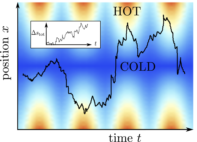
Figure 1: Spatial trajectory of a particle according to stochastic dynamics in the presence of an environment where the temperature varies in time and space, illustrated by the text and background colours. The evolution of the stochastic entropy production $\Delta s_{{\rm tot}}$ associated with the Brownian trajectory is sketched in the inset.

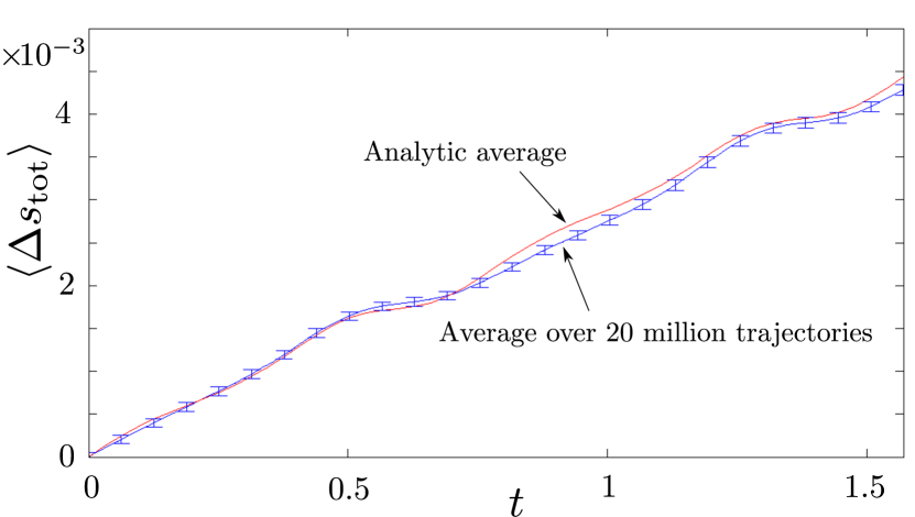
Figure 2: A comparison between the mean total stochastic entropy production obtained from the integral of the approximate Eq. (27) and the total stochastic entropy production averaged over $2\times 10^{7}$ numerically generated particle trajectories, each with 40000 timesteps, shown with error bars. The time interval represents two cycles of temperature variation, preceded in the simulations by one cycle to establish an evolving pdf similar to Eq. (21).

We choose simple forms of the potential and thermal background that the particle experiences. We consider a harmonic force $F(x)=-\kappa x$ where $\kappa$ is a spring constant, and an environmental temperature that varies in space and time according to

$$T_{r}(x,t)=T_{0}[1+\kappa_{T}(t)x^{2}/(2kT_{0})],$$ (28)

where $T_{0}$ is a constant and the time dependence is specified by $\kappa_{T}(t)=\kappa_{T}^{0}+B\sin\omega t>0$ with constant $B$. Four cycles of such behaviour are sketched in Figure 1. The environment is hotter as the distance from the particle tether point increases, and the spatial temperature profile varies sinusoidally with time. We expect heat to be carried by the particle, on average, from sources located away from the tether point towards sinks situated near the centre of the motion. The average rate of flow of heat should be affected by the time dependence of $T_{r}$.

This choice of profile implies that $T_{r}^{0}(x)=T_{0}[1+\kappa_{T}^{0}x^{2}/(2kT_{0})]$ and we evaluate the integral

$$\int_{0}^{x}dx\frac{F(x)}{kT_{r}^{0}(x)} = -\int_{0}^{x}dx\frac{\kappa x}{kT_{0}[1+\kappa_{T}^{0}x^{2}/(2kT_{0})]}$$ (29)

$$= -\left(\kappa/\kappa_{T}^{0}\right)\ln[1+\kappa_{T}^{0}x^{2}/(2kT_{0})],$$

such that the normalised stationary spatial pdf according to Eq. (15) is

$$\rho_{{\rm st}}(x)=\left(\frac{\kappa_{T}^{0}}{2\pi kT_{0}}\right)^{\frac{1}{2}}\frac{\Gamma\left(1+\kappa/\kappa_{T}^{0}\right)}{\Gamma\left(\frac{1}{2}+\kappa/\kappa_{T}^{0}\right)}\left[1+\frac{\kappa_{T}^{0}}{2kT_{0}}x^{2}\right]^{-1-\kappa/\kappa_{T}^{0}}$$ (30)

and furthermore we can write

$$\frac{\partial T_{r}}{\partial x}=\kappa_{T}(t)\frac{x}{k},$$ (31)

and

$$\frac{\partial T_{r}}{\partial t}=\frac{d\kappa_{T}(t)}{dt}\frac{x^{2}}{2k},$$ (32)

which fully specifies the evolution of $\langle\Delta s_{{\rm tot}}\rangle$ given in Eq. (27). A similar system with time-independent $\kappa_{T}$ was examined in Ford and Eyre (2015) for the purpose of deriving work relations under nonisothermal conditions.

For the numerical computation of the total entropy production we integrate

$$d\Delta s_{{\rm tot}}=-d[\ln p]-\frac{m}{2kT_{r}}d\left[v^{2}\right]-\frac{\kappa x}{kT_{r}}dx,$$ (33)

along with the SDEs for $x$ and $v$, and the components of entropy production evolve Spinney and Ford (2012b) according to

$$d\Delta s_{1} = -d[\ln p]+d[\ln p_{{\rm st}}],$$ (34)

$$d\Delta s_{3} = -d[\ln p_{{\rm st}}(x,v)]+d[\ln(p_{{\rm st}}(x,-v)],$$ (35)

together with $d\Delta s_{2}=d\Delta s_{{\rm tot}}-d\Delta s_{1}-d\Delta s_{3}$.

We select initial coordinates from the stationary pdf $p_{{\rm st}}(x,v)$ specified by $T_{r}^{0}(x)$, the temperature profile at $t=0$, and evolve the system over a time interval $0\leq t\leq 6\pi/\omega$ corresponding to three cycles of variation in the temperature profile, with parameters $\omega=8$, $m=1$, $kT_{0}=1$, $\kappa=1$, $\kappa_{T}^{0}=0.5$, $B=0.2$, and $\gamma=60$. The short relaxation time $\gamma^{-1}$ relative to the cycle period $2\pi/\omega$ ensures that the dynamics do not depart very far from the overdamped limit such that the expressions for $p$ and $p_{{\rm st}}$ given in Eqs. (21) and (22) are reasonably accurate.

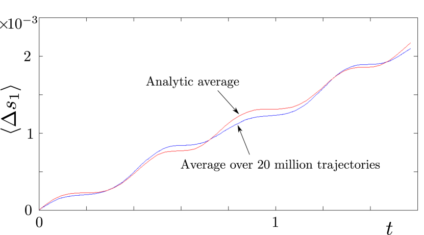
Figure 3: Comparison of the average of $\Delta s_{1}$ predicted analytically and calculated from the simulation of $2\times 10^{7}$ particle trajectories over a time interval of two temperature cycles preceded by one cycle to establish the periodic stationary state.

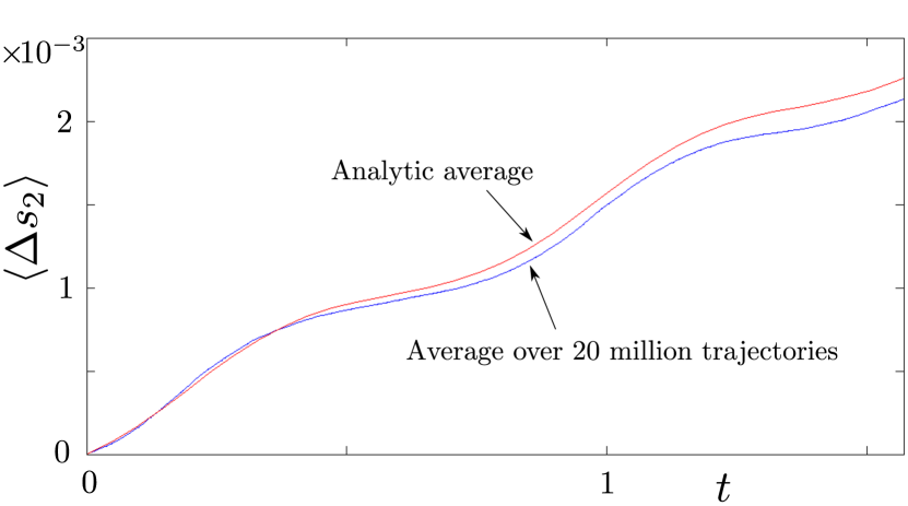
Figure 4: As Figure 3 but for the average of $\Delta s_{2}$.

The interval is divided into 40000 timesteps of length $\delta t=5.89\times 10^{-5}$ and samples of entropy production are generated from $2\times 10^{7}$ realisations of the Brownian motion. The system relaxes quickly into a periodic stationary state but we disregard behaviour taking place in the first cycle $0\leq t\leq 2\pi/\omega$ and focus our attention on entropy production during the second and third cycles.

We gauge the quality of the numerical calculations by checking that $\langle\Delta s_{{\rm tot}}\rangle$ matches the evolution obtained from integrating the approximate analytical expression (27). Statistical uncertainty in the numerical results is assessed by blocking the realisations into 40 subsets, and the resulting error bars in Figure 2 show that the accuracy of the numerical approach is satisfactory. Similar conclusions are reached by determining the evolution of $\langle\Delta s_{1}\rangle$ by the analytic and numerical routes, illustrated in Figure 3 and a similar procedure for $\langle\Delta s_{2}\rangle$ in Figure 4. The different character of these two components of entropy production is apparent. There are two bursts of relatively rapid mean production of $\Delta s_{1}$ per cycle. The system responds to the raising and lowering of the temperature profile and relaxational entropy generation is associated with both. In contrast, the time development of $\langle\Delta s_{2}\rangle$ more closely matches the periodicity of the temperature cycle, since it is a reflection of the entropy production that would characterise a stationary state for a given nonisothermal profile.

The $\Delta s_{1}$ and $\Delta s_{2}$ components of entropy production, as well as $\Delta s_{{\rm tot}}$, satisfy an integral fluctuation relation $\langle\exp(-\Delta s_{i})\rangle=1$ by construction for any elapsed time interval Esposito and Van den Broeck (2010a); Spinney and Ford (2012a). We can demonstrate further that a detailed fluctuation relation $P(\Delta s_{{\rm tot}})=P(-\Delta s_{{\rm tot}})\exp(\Delta s_{{\rm tot}})$ appears to be satisfied by $\Delta s_{{\rm tot}}$ for certain time intervals, as illustrated in Figure 5. We have chosen conditions where the initial and final system pdfs are the same, which will be the case for an interval that is a multiple of the cycle period $2\pi/\omega$ once the system has adopted a periodic stationary state; and for which the evolution of the environmental temperature profile is symmetric about the midpoint of the time interval, for example $7\pi/2\omega\leq t\leq 11\pi/2\omega$ indicated by the horizontal bar in the inset shown in Figure 5. These are circumstances where the total entropy production in a system described by spatial coordinates alone Harris and Schütz (2007); Spinney and Ford (2013) is expected to satisfy a detailed fluctuation relation. The backward version of the process in this time interval is identical to the forward version. Detailed fluctuation relations relate distributions of entropy production in forward and backward processes but here the two are synonymous. For time intervals where this is not the case, for example $3\pi/\omega\leq t\leq 5\pi/\omega$, the distribution of total entropy production will not satisfy a detailed fluctuation relation.

For systems that possess velocity coordinates, a detailed fluctuation relation for $\Delta s_{{\rm tot}}$ will be valid if, additionally, the initial pdf for the backward process is the time-reversed version of the initial pdf for the forward process. For such a relation to hold for our system, the pdf at the beginning and end of the cycle should be velocity symmetric, as demonstrated in Appendix D.1. This condition is not in general satisfied for a nonequilibrium system described by underdamped dynamics, but if the friction coefficient is not too small, the velocity asymmetry in Eq. (21) is slight and the detailed fluctuation relation should hold to a good approximation.

We found that the distribution of $\Delta s_{1}$ over the same time interval $7\pi/2\omega\leq t\leq 11\pi/2\omega$ also appears to satisfy a detailed fluctuation relation, as shown in Figure 6, while in contrast the distribution of $\Delta s_{2}$ does not possess such a symmetry, as illustrated in Figure 7. In Appendix D.2 we consider conditions for the existence of a detailed fluctuation relation for the $\Delta s_{1}$ component of entropy production in general systems with spatial and velocity coordinates. We conclude that $P(\Delta s_{1})$ will satisfy a detailed fluctuation relation if the friction coefficient is not too small, such that behaviour under the chosen system dynamics and its ‘adjoint’ version are simply related. A detailed fluctuation relation was observed for the total entropy production in a stationary state of thermal transport in Spinney and Ford (2012b), and this can now be interpreted as an approximate result. Furthermore, the conditions that allow us to show that detailed fluctuation relations hold to a certain extent for $P(\Delta s_{{\rm tot}})$ and $P(\Delta s_{1})$ do not imply a similar property for $P(\Delta s_{2})$, as shown in Appendix D.3, allowing us to understand the contrast in behaviour between Figures 5, 6 and 7.

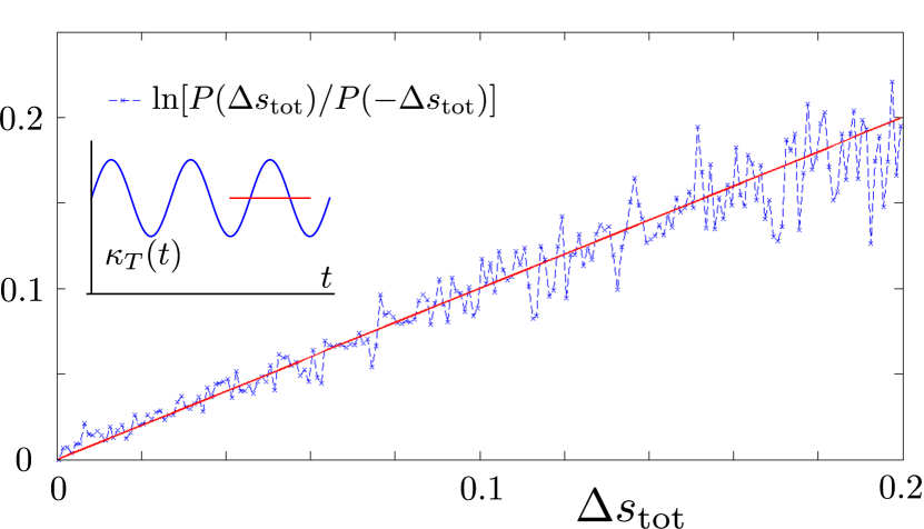
Figure 5: Numerical verification of an approximate detailed fluctuation relation for the pdf of total stochastic entropy production $\Delta s_{{\rm tot}}$ in the time interval $7\pi/2\omega\leq t\leq 11\pi/2\omega$ (shown as a bar in the inset), driven by the change in temperature profile according to the evolving $\kappa_{T}(t)$. Values of $\Delta s_{{\rm tot}}$ between $\pm 0.2$ from the simulation of $2\times 10^{7}$ particle trajectories are collected into 400 bins, and the straight line represents the outcome expected in the absence of sampling errors.

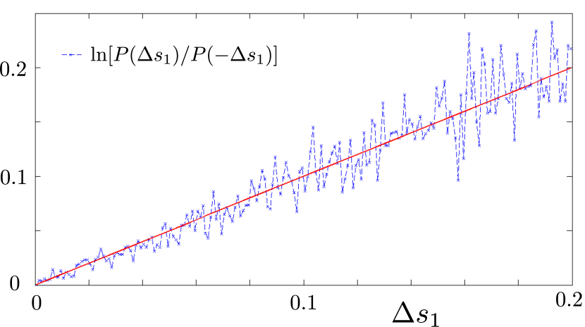
Figure 6: As Figure 5 but for $\Delta s_{1}$.

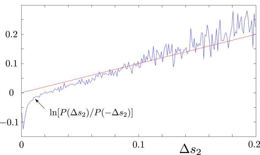
Figure 7: Demonstration that a detailed fluctuation relation does not appear to hold for $\Delta s_{2}$ in the interval $7\pi/2\omega\leq t\leq 11\pi/2\omega$.

Figure 8: Distributions of $\Delta s_{{\rm tot}}$, $\Delta s_{1}$, $\Delta s_{2}$ and $\Delta s_{3}$ generated in two cycles of temperature variation $2\pi/\omega\leq t\leq 6\pi/\omega$.

Distributions $P(\Delta s_{i})$ of the three components of entropy production generated over two cycles of the variation in temperature profile, namely for the interval $2\pi/\omega\leq t\leq 6\pi/\omega$, together with the distribution of their sum $\Delta s_{{\rm tot}}$, are shown in Figure 8. The fluctuations in the $\Delta s_{3}$ component are the smallest, but all contributions explore a broad range in comparison with their averages, which according to Figures 3 and 4 would be of order $10^{-3}$ for $\langle\Delta s_{1}\rangle$ and $\langle\Delta s_{2}\rangle$, together with $\langle\Delta s_{3}\rangle\approx 0$.

The second law in the stochastic framework corresponds to the non-negativity of the mean values of $\Delta s_{{\rm tot}}$, $\Delta s_{1}$ and $\Delta s_{2}$ over distributions such as these. Although the peak in the distribution of $\Delta s_{2}$ lies slightly to the left of the origin, its mean is positive as required. We have clearly demonstrated that there is considerable weight of probability for the generation of negative values of these quantities for this small system as it undergoes a short process. Nevertheless, such fluctuations are governed by rules in the form of fluctuation relations of various kinds. We have also demonstrated that the transient housekeeping component of entropy production $\Delta s_{3}$ associated with the breakage of the principle of detailed balance in a system evolving in full phase space makes a significant contribution to the total stochastic entropy production.

V Conclusions

The irreversibility of a stochastic process can be quantified through the consideration of three components of stochastic entropy production. In order to illustrate this we have studied the behaviour of a particle coupled to an environment characterised by a temperature that depends on time and space. The system is complex enough to manifest all three components of entropy production, and yet simple enough for us to obtain an approximate expression for the time dependent probability density function (pdf) of particle position and velocity that is required to perform the computations. In order to solve the Kramers equation and determine the pdf, we use a variational approach that resembles the maximisation of an Onsager function. Such an approach has been regarded as the use of a principle of maximisation of the rate of thermodynamic entropy production under constraints, but there is a certain ambiguity in the thermodynamic interpretation and we have discussed a point of view where it might instead be regarded as a constrained minimisation. A cautious thermodynamic interpretation is probably necessary.

Mean relaxational or nonadiabatic entropy production $\langle\Delta s_{1}\rangle$ is driven by the time dependence of the environmental temperature, and arises from the tendency of the system to evolve towards a state of local thermal equilibrium with respect to the environment, which here is frustrated by the continual environmental change. Mean housekeeping entropy production $\langle\Delta s_{2}\rangle$ is brought about by the spatial dependence of the environmental temperature, and is associated with the passage of heat, on average, from hotter to cooler parts of the environment by way of the particle. We have provided analytic expressions, correct to first order in inverse friction coefficient, for the evolution of the mean values of $\Delta s_{1}$ and $\Delta s_{2}$. The mean of the third component, the transient housekeeping entropy production $\Delta s_{3}$, is zero at the level of approximation employed, and in order to compute a nonzero mean for this quantity we would need to determine the system pdf to second order in inverse friction coefficient. The $\Delta s_{3}$ component contributes to the fluctuations in stochastic entropy production when the system is in a stationary state characterised by a velocity asymmetric pdf, and would be expected to have a nonzero mean when a system undergoes relaxation: it is therefore indicative of both relaxational and housekeeping behaviour.

We have determined the distributions of entropy production for certain time intervals, and investigated situations where both $\Delta s_{{\rm tot}}$ and $\Delta s_{1}$ satisfy a detailed fluctuation relation. Analysis given in Appendix D suggests that $\Delta s_{2}$ does not have this property in the same circumstances, and that the detailed fluctuation relations hold for the system and circumstances under consideration as long as the friction coefficient is not too small. Detailed fluctuation relations are a rightly celebrated centrepiece of the thermodynamics of small systems, since they express an asymmetry in the production and consumption of entropy, but they rely on the validity of certain initial and final conditions for the forward and backward processes considered, and we have illustrated this feature for a particular underdamped system. Finally, we have computed the distributions of the three components of entropy production, showing that in the case studied the $\Delta s_{3}$ component has a smaller variance than the other two.

The basis of the second law in stochastic thermodynamics is the adherence of $\Delta s_{{\rm tot}}$, $\Delta s_{1}$ and $\Delta s_{2}$ to integral fluctuation relations, and we have succeeded in demonstrating the consequent monotonic increase in the mean values of these forms of stochastic entropy production for a system processed in a way that gives rise to nonstationary thermal transport. We have also clearly demonstrated the existence of the third component $\Delta s_{3}$ in a situation where the stationary state of the system is asymmetric in velocity. These observations provide further illustration of the rich structure of stochastic thermodynamics.

Appendix A Components of stochastic entropy production

We summarise results that are derived in more detail in Spinney and Ford Spinney and Ford (2012b), concerning the dynamics of components of stochastic entropy production. For It$\bar{{\rm o}}$-rules stochastic differential equations (SDEs)

$$d{\rm x}_{i}=A_{i}(\textbf{x},t)dt+B_{i}(\textbf{x},t)dW_{i},$$ (36)

where x represents a set of dynamical variables $({\rm x_{1},{\rm x_{2},\cdots)}}$ such as $(x,v)$, we define

$$A_{i}^{{\rm ir}}(\textbf{x},t) = \frac{1}{2}\left[A_{i}(\textbf{x},t)+\varepsilon_{i}A_{i}(\boldsymbol{\varepsilon}\textbf{x},t)\right]=\varepsilon_{i}A_{i}^{{\rm ir}}(\boldsymbol{\varepsilon}\textbf{x},t),\qquad$$ (37)

and

$$A_{i}^{{\rm rev}}(\textbf{x},t)=\frac{1}{2}\left[A_{i}(\textbf{x},t)-\varepsilon_{i}A_{i}(\boldsymbol{\varepsilon}\textbf{x},t)\right]=-\varepsilon_{i}A_{i}^{{\rm rev}}(\boldsymbol{\varepsilon}\textbf{x},t),\quad$$ (38)

where $\varepsilon_{i}=1$ for variables ${\rm x}_{i}$ with even parity under time reversal symmetry (for example position $x$) and $\varepsilon_{i}=-1$ for variables with odd parity (for example velocity $v$), and $\boldsymbol{\varepsilon}\textbf{x}$ represents $(\varepsilon_{1}{\rm x_{1},\varepsilon_{2}{\rm x_{2},\cdots)}}$. Defining also $D_{i}(\textbf{x},t)=\frac{1}{2}B_{i}(\textbf{x},t)^{2}$, it may be shown that the following It$\bar{{\rm o}}$-rules SDE for the total entropy production (defined in Eq. (3)) emerges:

$$d\Delta s_{{\rm tot}}=-d(\ln p)+\sum_{i}\frac{A_{i}^{{\rm ir}}}{D_{i}}d{\rm x}_{i}-\frac{A_{i}^{{\rm rev}}A_{i}^{{\rm ir}}}{D_{i}}dt+\frac{\partial A_{i}^{{\rm ir}}}{\partial{\rm x}_{i}}dt$$

$$-\frac{\partial A_{i}^{{\rm rev}}}{\partial{\rm x}_{i}}dt-\frac{1}{D_{i}}\frac{\partial D_{i}}{\partial{\rm x}_{i}}d{\rm x}_{i}+\frac{(A_{i}^{{\rm rev}}-A_{i}^{{\rm ir}})}{D_{i}}\frac{\partial D_{i}}{\partial{\rm x}_{i}}dt$$

$$-\frac{\partial^{2}D_{i}}{\partial{\rm x}_{i}^{2}}dt+\frac{1}{D_{i}}\left(\frac{\partial D_{i}}{\partial{\rm x}_{i}}\right)^{2}dt,\quad$$ (39)

where $p$ is the time dependent pdf of variables x. The corresponding It$\bar{{\rm o}}$ SDE for the principal relaxational entropy production is

$$d\Delta s_{1}=-d(\ln p)-\frac{\partial\varphi}{\partial{\rm x}_{i}}d{\rm x}_{i}-D_{i}\frac{\partial^{2}\varphi}{\partial{\rm x}_{i}^{2}}dt,$$ (40)

where $\varphi=-\ln p_{{\rm st}}$ and $p_{{\rm st}}$ is the stationary pdf. We also have

$$d\Delta s_{2}=\sum_{i}-\frac{A_{i}^{{\rm ir}}A_{i}^{{\rm rev}}}{D_{i}}dt+\frac{A_{i}^{{\rm ir}}}{D_{i}}d{\rm x}_{i}+\varepsilon_{i}\varphi_{i}^{\prime}(\boldsymbol{\varepsilon}\textbf{x})d{\rm x}_{i}$$

$$-\frac{1}{D_{i}}\frac{\partial D_{i}}{\partial{\rm x}_{i}}d{\rm x}_{i}+\frac{1}{D_{i}}\left(\frac{\partial D_{i}}{\partial{\rm x}_{i}}\right)^{2}dt+D_{i}(\varphi_{i}^{\prime}(\boldsymbol{\varepsilon}\textbf{x}))^{2}dt$$

$$-2\varepsilon_{i}\varphi_{i}^{\prime}(\boldsymbol{\varepsilon}\textbf{x})\frac{\partial D_{i}}{\partial{\rm x}_{i}}dt+\varepsilon_{i}(A_{i}^{{\rm ir}}-A_{i}^{{\rm rev}})\varphi_{i}^{\prime}(\boldsymbol{\varepsilon}\textbf{x})dt$$

$$-\frac{(A_{i}^{{\rm ir}}-A_{i}^{{\rm rev}})}{D_{i}}\frac{\partial D_{i}}{\partial{\rm x}_{i}}dt,$$ (41)

specifying an increment in $\Delta s_{2}$, using notation $\varphi_{i}^{\prime}(\boldsymbol{\varepsilon}\textbf{x})=\varepsilon_{i}\partial\varphi(\boldsymbol{\varepsilon}\textbf{x})/\partial{\rm x}_{i}$ and

$$d\Delta s_{3} = -d\ln p_{{\rm st}}(\textbf{x})+d\ln p_{{\rm st}}(\boldsymbol{\varepsilon}\textbf{x})$$ (42)

$$= \sum_{i}\varphi_{i}^{\prime}(\textbf{x})\circ d{\rm x}_{i}-\varepsilon_{i}\varphi_{i}^{\prime}(\boldsymbol{\varepsilon}\textbf{x})\circ d{\rm x}_{i},$$

for the third component. Stratonovich notation is used in the second line for reasons of compactness, but a more elaborate It$\bar{{\rm o}}$-rules version can be constructed. For the dynamics specified by Eqs. (1) and (2) we have $A_{x}^{{\rm ir}}=0$, $A_{x}^{{\rm rev}}=v$, $A_{v}^{{\rm ir}}=-\gamma v$, $A_{v}^{{\rm rev}}=F/m$, $D_{x}=0$ and $D_{v}=kT_{r}\gamma/m$ and using Eq. (39) we recover Eq. (3).

Appendix B Variational solution to the Kramers equation

We wish to obtain a solution to the approximate Kramers equation

$$\frac{\partial f}{\partial t}+v\frac{\partial f}{\partial x}+\left(\frac{F}{m}-\gamma\bar{v}\right)\frac{\partial f}{\partial v}=\frac{kT_{r}\gamma}{m}\frac{\partial}{\partial v}\left(f\frac{\partial(\gamma^{-1}\psi_{1})}{\partial v}\right),$$ (43)

that results from inserting Eq. (13) into Eq. (16) without setting $\rho=\rho_{{\rm st}}$ or $\bar{v}=0$, and using the leading term in Eq. (17). For simplicity of notation we henceforth write $\psi=\gamma^{-1}\psi_{1}$. The approach involves a variational principle employed for a similar purpose by Kohler Kohler (1948), Ziman Ziman (1956) and Cercignani Cercignani (2000), and which has been discussed in a broader context by Martyushev and Seleznev Martyushev and Seleznev (2006). Casting Eq. (43) in the form $Z=\hat{L}\psi$ where $\hat{L}$ is the linear operator given by $\hat{L}(\cdot)=(kT_{r}\gamma/m)\partial/\partial v(f\partial(\cdot)/\partial v)$, we seek a solution by extremising the functional

$$I[\tilde{\psi}]=-(\tilde{\psi},Z)+\frac{1}{2}(\tilde{\psi},\hat{L}\tilde{\psi})$$ (44)

over trial solutions $\tilde{\psi}$ that satisfy relevant constraints $\int dvf\tilde{\psi}=0$ and $\int dvvf\tilde{\psi}=0$. The meaning of the brackets is $(A,B)=\int dvAB$ such that

$$(\tilde{\psi},\hat{L}\tilde{\psi}) = \int dv\tilde{\psi}\frac{kT_{r}\gamma}{m}\frac{\partial}{\partial v}\left(f\frac{\partial\tilde{\psi}}{\partial v}\right)$$ (45)

$$= -\int dv\frac{\partial\tilde{\psi}}{\partial v}\frac{kT_{r}\gamma}{m}f\frac{\partial\tilde{\psi}}{\partial v}.$$

The approach can be justified by writing $\tilde{\psi}=\psi+\eta$ in which case it may be shown that

$$I[\tilde{\psi}] = I[\psi]+\frac{1}{2}(\eta,\hat{L}\eta),$$ (46)

as long as $\hat{L}$ satisfies $(\hat{L}\psi,\eta)=(\psi,\hat{L}\eta)$. It is clear from Eq. (45) that $(\eta,\hat{L}\eta)$ for the operator $\hat{L}$ in question is never positive, so the variational principle may be characterised as the maximisation of $I[\tilde{\psi}]$, which is achieved when $\tilde{\psi}=\psi$. The value of the functional in such a circumstance is

$$I[\psi]=\frac{1}{2}(\psi,\hat{L}\psi)-(\psi,Z)=-\frac{1}{2}(\psi,\hat{L}\psi)\geq 0.$$ (47)

We clearly need to evaluate

$$(\tilde{\psi},Z)=\int\!dv\tilde{\psi}\frac{\partial f}{\partial t}+\int dv\tilde{\psi}v\frac{\partial f}{\partial x}+\int dv\tilde{\psi}\left(\frac{F}{m}-\gamma\bar{v}\right)\frac{\partial f}{\partial v},$$ (48)

and for the first term we write

$$\int dv\ \tilde{\psi}\frac{\partial f}{\partial t}=\int dv\ \tilde{\psi}\left[\frac{\partial\rho}{\partial t}\frac{f}{\rho}-\frac{f}{2T_{r}}\frac{\partial T_{r}}{\partial t}\right.$$

$$\left.+f\left(\frac{m(v-\bar{v})}{kT_{r}}\frac{\partial\bar{v}}{\partial t}+\frac{m(v-\bar{v})^{2}}{2kT_{r}^{2}}\frac{\partial T_{r}}{\partial t}\right)\right]$$

$$=\int dv\ \tilde{\psi}f\left(\frac{m(v-\bar{v})^{2}}{2kT_{r}^{2}}\frac{\partial T_{r}}{\partial t}\right),$$ (49)

having used $\int dvf\tilde{\psi}=0$ and $\int dvvf\tilde{\psi}=0$. For the second term we get

$$\int dv\ \tilde{\psi}v\frac{\partial f}{\partial x}=\int dv\ \tilde{\psi}v\left[\frac{\partial\rho}{\partial x}\frac{f}{\rho}-\frac{f}{2T_{r}}\frac{\partial T_{r}}{\partial x}\right.$$

$$\left.+f\left(\frac{m(v-\bar{v})}{kT_{r}}\frac{\partial\bar{v}}{\partial x}+\frac{m(v-\bar{v})^{2}}{2kT_{r}^{2}}\frac{\partial T_{r}}{\partial x}\right)\right]$$

$$=\int dv\ \tilde{\psi}vf\left(\frac{mv}{kT_{r}}\frac{\partial\bar{v}}{\partial x}+\frac{m(v-\bar{v})^{2}}{2kT_{r}^{2}}\frac{\partial T_{r}}{\partial x}\right),$$ (50)

and by similar reasoning the third term in Eq. (48) vanishes. We therefore find that

$$I[\tilde{\psi}]=-\frac{1}{2}\int\!\!dv\frac{\partial\tilde{\psi}}{\partial v}\frac{kT_{r}\gamma}{m}f\frac{\partial\tilde{\psi}}{\partial v}-\frac{m}{2kT_{r}^{2}}\frac{\partial T_{r}}{\partial t}\!\int\!\!dv\tilde{\psi}f(v-\bar{v}){}^{2}$$

$$-\int dv\tilde{\psi}vf\left(\frac{m(v-\bar{v})}{kT_{r}}\frac{\partial\bar{v}}{\partial x}+\frac{m(v-\bar{v})^{2}}{2kT_{r}^{2}}\frac{\partial T_{r}}{\partial x}\right),$$ (51)

is the expression that has to be maximised over $\tilde{\psi}$ subject to $\int dv\tilde{\psi}f=0$ and $\int dvv\tilde{\psi}f=0$.

The Euler-Lagrange equation that specifies the optimal $\psi$ is

$$-\frac{kT_{r}\gamma}{m}\frac{\partial}{\partial v}f\frac{\partial\psi}{\partial v}=\lambda_{1}f+\lambda_{2}vf-\frac{m}{2kT_{r}^{2}}\frac{\partial T_{r}}{\partial t}f(v-\bar{v}){}^{2}$$

$$-vf\left(\frac{m(v-\bar{v})}{kT_{r}}\frac{\partial\bar{v}}{\partial x}+\frac{m(v-\bar{v})^{2}}{2kT_{r}^{2}}\frac{\partial T_{r}}{\partial x}\right)$$

$$=-\frac{kT_{r}\gamma}{m}\left(-\frac{\partial\psi}{\partial v}\frac{m(v-\bar{v})}{kT_{r}}f+f\frac{\partial^{2}\psi}{\partial v^{2}}\right),$$ (52)

where Lagrange multipliers $\lambda_{1,2}$ associated with the constraints appear. Inserting a trial solution

$$\psi=\psi_{0}+a(v-\bar{v})+b(v-\bar{v})^{2}+c(v-\bar{v})^{3},$$ (53)

we get

$$\lambda_{1}+\lambda_{2}(z+\bar{v})-\frac{m}{2kT_{r}^{2}}\frac{\partial T_{r}}{\partial t}z^{2}$$

$$-(z+\bar{v})\left(\frac{mz}{kT_{r}}\frac{\partial\bar{v}}{\partial x}+\frac{mz^{2}}{2kT_{r}^{2}}\frac{\partial T_{r}}{\partial x}\right)$$

$$=\frac{kT_{r}\gamma}{m}\left(\left(a+2bz+3cz^{2}\right)\frac{mz}{kT_{r}}-2b-6cz\right),\qquad$$ (54)

where $z=v-\bar{v}$, and by requiring that the coefficients of $z^{2}$ and $z^{3}$ be zero together with imposing $\int dv\psi f=\int dvv\psi f=0$, we obtain

$$a = \frac{1}{2\gamma T_{r}}\frac{\partial T_{r}}{\partial x}$$

$$b = -\frac{m}{4kT_{r}\gamma}\left(\frac{1}{T_{r}}\frac{\partial T_{r}}{\partial t}+2\frac{\partial\bar{v}}{\partial x}+\frac{\bar{v}}{T_{r}}\frac{\partial T_{r}}{\partial x}\right)$$

$$c = -\frac{m}{6\gamma kT_{r}^{2}}\frac{\partial T_{r}}{\partial x}$$

$$\psi_{0} = \frac{1}{4\gamma}\left(\frac{1}{T_{r}}\frac{\partial T_{r}}{\partial t}+2\frac{\partial\bar{v}}{\partial x}+\frac{\bar{v}}{T_{r}}\frac{\partial T_{r}}{\partial x}\right),$$ (55)

which specifies the approximate nonequilibrium pdf $p=f(1+\psi)$ for transient conditions. If we make the further approximations $\bar{v}=0$ and $\rho\approx\rho_{{\rm st}}$, this reduces to the solution given in Eq. (21).

Appendix C Rate of entropy production and Onsager’s principle

We discuss the relationship between the variational approach to solving the Kramers equation reviewed in Appendix B and proposals for identifying a nonequilibrium stationary state based on extremising the rate of thermodynamic entropy production. Such a principle has been discussed many times before Dewar (2003); Martyushev and Seleznev (2006). The version that is most appropriate in the present context is the maximisation of the Onsager function, the difference between the rate of entropy production and a quantity denoted the dissipation function Onsager (1931). In classical nonequilibrium thermodynamics, the rate of entropy production $\dot{S}(\{{\cal F}_{i},\tilde{J}_{i}\})$ is given by $\sum{\cal F}_{i}\tilde{J}_{i}$, in terms of currents $\tilde{J}_{i}$ (such as the heat flux or a particle current) and their respective driving thermodynamic forces ${\cal F}_{i}$ (gradients in the inverse temperature field and the negative of the chemical potential, respectively). The dissipation function is defined as $\frac{1}{2}\sum\tilde{J}_{i}L_{ij}\tilde{J}_{j}$ where the $L_{ij}$ is a matrix of coefficients. Maximisation of the Onsager function

$$\Omega(\{\tilde{J}_{i}\})=\sum{\cal F}_{i}\tilde{J}_{i}-\sum\frac{1}{2}\tilde{J}_{i}L_{ij}\tilde{J}_{j},$$ (56)

over currents $\tilde{J}_{i}$ for a given set of forces ${\cal F}_{i}$ produces linear relationships between the two in the form $\tilde{J}_{i}\to J_{i}=\sum R_{ij}{\cal F}_{j}$, where $R=L^{-1}$, in agreement with the phenomenological linear response, and hence provides a description of a nonequilibrium state. This has been referred to as Onsager’s principle and interpreted as the constrained maximisation of the rate of production of entropy. The maximised value of the Onsager function is $\frac{1}{2}\sum{\cal F}_{i}J_{i}$ [namely, half the rate of entropy production $\dot{S}(\{{\cal F}_{i},J_{i}\})=\sum{\cal F}_{i}J_{i}$] if it is assumed that such linear relationships prevail, and the dissipation function then takes the value $\frac{1}{2}\sum J_{i}L_{ij}J_{j}=\frac{1}{2}\sum{\cal F}_{i}J_{i}$. The formalism written here in terms of summations could be taken to apply to integrations over spatially dependent currents and forces. However, the origin of the dissipation function and the basis of the variational procedure are not altogether apparent.

Kohler Kohler (1948) and Ziman Ziman (1956) noticed the similarity between the Onsager function $\Omega(\{\tilde{J}_{i}\})$ and the variational functional $I[\tilde{\psi}]$ used in the solution of the stochastic dynamics in Appendix B and suggested that the latter provided a microscopic dynamical underpinning of Onsager’s principle. However, the latter is clearly founded upon a classical thermodynamic viewpoint where the primary representation of entropy production is the product of forces and currents. In contrast, in traditional statistical mechanics and in stochastic thermodynamics the primary representation is given in terms of properties of the system pdf. We can demonstrate this for the system under consideration in this study. By multiplying Eq. (5) by $-\ln p$ and integrating, we obtain after some manipulation

$$\frac{\partial\rho_{s}}{\partial t}+\frac{\partial j_{s}}{\partial x}=\int dv\frac{\partial\ln(1+\psi)}{\partial v}\frac{kT_{r}\gamma}{m}f\frac{\partial\psi}{\partial v}+\frac{\gamma\rho\left(T_{r}-T\right)}{T_{r}},$$ (57)

where $\psi$ specifies the pdf that satisfies the Kramers equation, and $\rho_{s}(x)=-\int dvp\ln p$ and $j_{s}(x)=-\int dvvp\ln p$ can be regarded as the density and current of (dimensionless) mean system entropy, respectively. We define the local temperature of the system $T(x,t)$ through $\int dv(v-\bar{v})^{2}p=\rho(\overline{v^{2}}-\bar{v}^{2})=kT\rho/m$. The final term in Eq. (57) corresponds to a Clausius-style entropy flow to the system associated with heat transfer from the environment brought about by the difference between $T_{r}$ and $T$. We can therefore identify the spatial density of the rate of entropy production from a statistical mechanical perspective, valid for transient as well as stationary situations, as

$$q_{s} \approx \int dv\frac{\partial\psi}{\partial v}\frac{kT_{r}\gamma}{m}f\frac{\partial\psi}{\partial v},$$ (58)

to leading order in inverse friction coefficient, which corresponds to $\bar{v}=0$ and $\psi\ll 1$. Notice that $q_{s}$ is therefore related to the quantity

$$-(\psi,\hat{L}\psi) = -\int dv\psi\frac{kT_{r}\gamma}{m}\frac{\partial}{\partial v}\left(f\frac{\partial\psi}{\partial v}\right)\approx q_{s}(\psi),\qquad$$ (59)

using the notation of Appendix B.

This interpretation may be demonstrated more directly from the expression for the mean rate of stochastic entropy production, $d\langle\Delta s_{{\rm tot}}\rangle/dt$ in Eq. (10). We have

$$\frac{d\langle\Delta s_{{\rm tot}}\rangle}{dt}=\int dxdv\frac{m}{pkT_{r}\gamma}\left(J_{v}^{{\rm ir}}\right)^{2}$$

$$=\int dxdv\left[\frac{\partial\ln(1+\psi)}{\partial v}\frac{kT_{r}\gamma}{m}f\frac{\partial\psi}{\partial v}+\frac{m}{kT_{r}}\gamma\rho\bar{v}^{2}\right],\quad$$ (60)

which for $\bar{v}=0$ and $\psi\ll 1$ reduces to the spatial integral of $q_{s}$ given by Eq. (58). This formulation emphasises that $q_{s}$ represents the spatial density of mean stochastic entropy production for any function $\psi$ and associated pdf $p$.

These considerations provide a thermodynamic interpretation of the $-(\tilde{\psi},\hat{L}\tilde{\psi})$ term in the functional $I[\tilde{\psi]}$ but they imply an important change in perspective. The variational principle can also be cast as the minimisation of $-2I[\tilde{\psi}]=-(\tilde{\psi},\hat{L}\tilde{\psi})+2(\tilde{\psi},Z)=q_{s}(\tilde{\psi})+2(\tilde{\psi},Z)$, which would then be regarded as a minimisation of the spatial density of the mean rate of stochastic entropy production $q_{s}(\tilde{\psi})$ with respect to the trial function $\tilde{\psi}$, under the constraint of a fixed value of $(\tilde{\psi},Z)$. By identifying the optimal trial function variationally, we are able to determine the solution to the Kramers equation. As noted by Kohler, Ziman and others, such an approach essentially provides a thermodynamic shortcut to solving the dynamical problem.

The negative of the expression $(\tilde{\psi},Z)$, when restricted to a stationary state with $\partial T_{r}/\partial t=0$ and $\bar{v}=0$, is given by

$$-(\tilde{\psi},Z) \approx -\frac{\partial T_{r}}{\partial x}\int dv\tilde{\psi}f\frac{mv^{3}}{2kT_{r}^{2}}$$ (61)

$$= \frac{\partial(T_{r}^{-1})}{\partial x}\int dv\left[f+\tilde{\psi}f\right]\frac{mv^{3}}{2k},$$

which is the product of the gradient of inverse temperature and the particle kinetic energy flux (divided by $k$) at position $x$, therefore resembling the spatial density of an entropy production rate in classical thermodynamics, for a trial $\tilde{\psi}$. However, in the context of stochastic thermodynamics $-(\tilde{\psi},Z)$ is not to be primarily identified as the entropy production, whereas $q_{s}$ most definitely can be so interpreted.

We have followed Kohler and Ziman in regarding the variational procedure used in Appendix B as a principle founded in dynamics (i.e. $\tilde{\psi}$ is selected in order to satisfy the Kramers equation) but which is capable of a thermodynamic interpretation. However, the apparent thermodynamic principle in operation is not quite as clear as has been suggested. The semantic subtlety is whether, following Onsager, we must maximise classical entropy production $\sum{\cal F}_{i}\tilde{J}_{i}$, subject to a fixed dissipation function $\frac{1}{2}\sum\tilde{J}_{i}L_{ij}\tilde{J}_{j}$, over currents $\tilde{J_{i}}$ for a given set of forces ${\cal F}_{i}$, or minimise a stochastic thermodynamic representation of the spatial density of entropy production, in this case $q_{s}(\tilde{\psi})$, with respect to a function $\tilde{\psi}$ subject to a fixed $(\tilde{\psi},Z)$. The fact that both interpretations can be maintained, depending on whether we use a classical or a stochastic framework of entropy production, suggests that taking a particular thermodynamic viewpoint of the procedure should be treated with caution.

Appendix D Detailed fluctuation relations

D.1 Detailed fluctuation relation for $\Delta s_{{\rm tot}}$

The total entropy production associated with a trajectory takes the form

$$\Delta s_{{\rm tot}}^{{\rm F}}[\boldsymbol{X}]=\ln\left[\frac{p_{{\rm start}}^{{\rm F}}[X(0)]{\cal P}^{{\rm F}}[X(\tau)|X(0)]}{p_{{\rm end}}^{{\rm F}}[X(\tau)]{\cal P}^{{\rm R}}[X^{\dagger}(\tau)|X^{\dagger}(0)]}\right],$$ (62)

where $\boldsymbol{X}$ corresponds to $\vec{\boldsymbol{x}},\vec{\boldsymbol{v}}$ and $X(t)$ represents the coordinates $x(t),v(t)$ taken by the system under what we shall call a forward protocol of driving, while $\boldsymbol{X}^{\dagger}$ corresponds to $\vec{\boldsymbol{x}}^{\dagger},\vec{\boldsymbol{v}}^{\dagger}$ with $X^{\dagger}(t)$ representing $x^{\dagger}(t),v^{\dagger}(t)$ where $x^{\dagger}(t)=x(\tau-t)$ and $v^{\dagger}(t)=-v(\tau-t)$. The superscript R indicates driving according to the reverse of the protocol that operates in the forward process, which is labelled F. The above expression is compatible with Eq. (3) with ${\rm P^{{\rm F}}}[\vec{\boldsymbol{x}},\vec{\boldsymbol{v}}]$ here explicitly written as $p_{{\rm start}}^{{\rm F}}[X(0)]{\cal P}^{{\rm F}}[X(\tau)|X(0)]$ in terms of a pdf of initial coordinates $p_{{\rm start}}^{{\rm F}}$ and a conditional probability density ${\cal P}^{{\rm F}}$. Note that the expression takes the form of a ratio of probabilities of a trajectory and a (nominal) reverse or antitrajectory, the initial pdf of which is $p_{{\rm end}}^{{\rm F}}[X(\tau)]$, the pdf of coordinates at the end of the forward trajectory. There is an implied inversion Ford (2015) of the velocity coordinate such that $X(\tau)\to X^{\dagger}(0)$ before the continuation with the reverse trajectory $X^{\dagger}(0)\to X^{\dagger}(\tau)$. The pdf of initial coordinates for the reverse trajectory is therefore determined by the forward process.

The distribution of entropy production for the forward process can be written as

$$P^{{\rm F}}(\Delta s_{{\rm tot}}^{{\rm F}}=A)$$ (63)

$$=\int d\boldsymbol{X}\;p_{{\rm start}}^{{\rm F}}[X(0)]{\cal P}^{{\rm F}}[X(\tau)|X(0)]\delta(A-\Delta s_{{\rm tot}}^{{\rm F}}[\boldsymbol{X}]),$$

and this depends on the form taken by the initial pdf, and the nature of the prevailing dynamics.

We next consider the entropy production for a trajectory generated in a process starting from a pdf $p_{{\rm start}}^{{\rm R}}$ and driven by a reverse protocol. This is

$$\Delta s_{{\rm tot}}^{{\rm R}}[\bar{\boldsymbol{X}}]=\ln\left[\frac{p_{{\rm start}}^{{\rm R}}[\bar{X}(0)]{\cal P}^{{\rm R}}[\bar{X}(\tau)|\bar{X}(0)]}{p_{{\rm end}}^{{\rm R}}[\bar{X}(\tau)]{\cal P}^{{\rm F}}[\bar{X}^{\dagger}(\tau)|\bar{X}^{\dagger}(0)]}\right].$$ (64)

The trajectory shown here is general but it will prove fruitful to write $\bar{\boldsymbol{X}}$ as $\boldsymbol{X}^{\dagger}$ and therefore related to $\boldsymbol{X}$, i.e. $\bar{X}(0)$ represents $x(\tau),-v(\tau)$; $\bar{X}(\tau)$ is $x(0),-v(0)$; $\bar{X}^{\dagger}(0)$ represents $x(0),v(0)$ or $X(0)$; and $\bar{X}^{\dagger}(\tau)$ is $x(\tau),v(\tau)$ or $X(\tau)$. Clearly this specification of $\bar{\boldsymbol{X}}$ satisfies the dynamics under reverse driving. We have

$$\Delta s_{{\rm tot}}^{{\rm R}}[\boldsymbol{X}^{\dagger}] = \ln\left[\frac{p_{{\rm start}}^{{\rm R}}[X^{\dagger}(0)]{\cal P}^{{\rm R}}[X^{\dagger}(\tau)|X^{\dagger}(0)]}{p_{{\rm end}}^{{\rm R}}[X^{\dagger}(\tau)]{\cal P}^{{\rm F}}[X(\tau)|X(0)]}\right],\quad$$ (65)

and we compute the distribution of total entropy production in this process:

$$P^{{\rm R}}(\Delta s_{{\rm tot}}^{{\rm R}}=A)$$ (66)

$$\!=\!\int\!d\boldsymbol{X}^{\dagger}p_{{\rm start}}^{{\rm R}}[X^{\dagger}(0)]{\cal P}^{{\rm R}}[X^{\dagger}(\tau)|X^{\dagger}(0)]\delta(A-\Delta s_{{\rm tot}}^{{\rm R}}[\boldsymbol{X}^{\dagger}]).$$

Writing Eq. (65) in the form

$$p_{{\rm start}}^{{\rm R}}[X^{\dagger}(0)]{\cal P}^{{\rm R}}[X^{\dagger}(\tau)|X^{\dagger}(0)]$$

$$=p_{{\rm end}}^{{\rm R}}[X^{{\rm\dagger}}(\tau)]{\cal P}^{{\rm F}}[X(\tau)|X(0)]{\rm e}^{\Delta s_{{\rm tot}}^{{\rm R}}[\boldsymbol{X}^{\dagger}]},$$ (67)

and noting that $d\boldsymbol{X}=d\boldsymbol{X}^{\dagger}$, we find that

$$P^{{\rm R}}(\Delta s_{{\rm tot}}^{{\rm R}}=A)=\int d\boldsymbol{X}^{\dagger}\;p_{{\rm end}}^{{\rm R}}[X^{{\rm\dagger}}(\tau)]{\cal P}^{{\rm F}}[X(\tau)|X(0)]$$

$$\qquad\times{\rm e}^{\Delta s_{{\rm tot}}^{{\rm R}}[\boldsymbol{X}^{\dagger}]}\delta(A-\Delta s_{{\rm tot}}^{{\rm R}}[\boldsymbol{X}^{\dagger}])$$ (68)

$$\!\!={\rm e}^{A}\int d\boldsymbol{X}p_{{\rm end}}^{{\rm R}}[X^{{\rm\dagger}}(\tau)]{\cal P}^{{\rm F}}[X(\tau)|X(0)]\delta(A-\Delta s_{{\rm tot}}^{{\rm R}}[\boldsymbol{X}^{\dagger}]).$$

Now, if it can be arranged that $p_{{\rm end}}^{{\rm R}}[X^{\dagger}(\tau)]=p_{{\rm start}}^{{\rm F}}[X(0)]$ or $p_{{\rm end}}^{{\rm R}}[x,-v]=p_{{\rm start}}^{{\rm F}}[x,v]$; and $p_{{\rm start}}^{{\rm R}}[X^{{\rm\dagger}}(0)]=p_{{\rm end}}^{{\rm F}}[X(\tau)]$ or $p_{{\rm start}}^{{\rm R}}[x,-v]=p_{{\rm end}}^{{\rm F}}[x,v]$, then it would follow that

$$\Delta s_{{\rm tot}}^{{\rm R}}[\boldsymbol{X}^{\dagger}] = \ln\left[\frac{p_{{\rm end}}^{{\rm F}}[X(\tau)]{\cal P}^{{\rm R}}[X^{\dagger}(\tau)|X^{\dagger}(0)]}{p_{{\rm start}}^{{\rm F}}[X(0)]{\cal P}^{{\rm F}}[X(\tau)|X(0)]}\right]$$ (69)

$$= -\Delta s_{{\rm tot}}^{{\rm F}}[\boldsymbol{X}],$$

in which case we would obtain the detailed fluctuation relation

$$P^{{\rm R}}(\Delta s_{{\rm tot}}^{{\rm R}}=A)=$$

$${\rm e}^{A}\!\int d\boldsymbol{X}\,p_{{\rm start}}^{{\rm F}}[X(0)]{\cal P}^{{\rm F}}[X(\tau)|X(0)]\delta(A+\Delta s_{{\rm tot}}^{{\rm F}}[\boldsymbol{X}])$$

$$={\rm e}^{A}\,P^{{\rm F}}(\Delta s_{{\rm tot}}^{{\rm F}}=-A).$$ (70)

It is necessary to state clearly what this means. It relates the pdf of total entropy production in a forward process to the pdf of total entropy production when the system is driven by a reverse protocol instead, with the condition that the initial pdf for the reverse process is a velocity inverted version of the final pdf in the forward process, and similarly the initial pdf for the forward process is a velocity inverted version of the final pdf from the reverse process. We have essentially followed Harris and Schütz (2007) and Shargel (2010) in this derivation.

A single system can be subjected to a forward and reverse process sequentially such that $p_{{\rm start}}^{{\rm R}}[x,v]=p_{{\rm end}}^{{\rm F}}[x,v]$ but the condition for the detailed fluctuation relation to hold would then require the pdf at the end of the forward sequence to be velocity symmetric. For a system driven by a repeated sequence of forward and reverse processes, $p_{{\rm start}}^{{\rm F}}[x,v]=p_{{\rm end}}^{{\rm R}}[x,v]$ would apply as well, implying velocity symmetry in the pdf at the end of the reverse sequence. Furthermore, if the forward and reverse protocols are identical, which requires each to be symmetric about the midpoint in the interval, the condition for the validity of the detailed fluctuation relation requires the initial and final pdfs to be the same, in which case Eq. (70) would reduce to

$$P(\Delta s_{{\rm tot}})={\rm e}^{\Delta s_{{\rm tot}}}\,P(-\Delta s_{{\rm tot}}),$$ (71)

for such an interval, which is the detailed fluctuation relation that is tested in Section IV. The required velocity symmetry of the pdf at the beginning and end of the interval does not hold in general, and indeed is not satisfied by $p(x,v,t)$ in Eq. (21) for the particular system we have studied, but for large $\gamma$ the asymmetry is small and in such circumstances Eq. (71) will apply to an approximate extent.

D.2 Detailed fluctuation relation for $\Delta s_{1}$

We can perform a similar analysis to find conditions for which the relaxational entropy production satisfies a detailed fluctuation relation. We start with the definition Chernyak et al. (2006); Spinney and Ford (2012b)

$$\Delta s_{1}^{{\rm F}}[\boldsymbol{X}]=\ln\left[\frac{p_{{\rm start}}^{{\rm F}}[X(0)]{\cal P}^{{\rm F}}[X(\tau)|X(0)]}{p_{{\rm end}}^{{\rm F}}[X(\tau)]{\cal P}_{{\rm ad}}^{{\rm R}}[X^{{\rm R}}(\tau)|X^{{\rm R}}(0)]}\right],$$ (72)

where $\boldsymbol{X}^{{\rm R}}$ corresponds to $\vec{\boldsymbol{x}}^{{\rm R}},\vec{\boldsymbol{v}}^{{\rm R}}$ with $X^{{\rm R}}(t)$ representing $x^{{\rm R}}(t),v^{{\rm R}}(t)$ where $x^{{\rm R}}(t)=x(\tau-t)$ and $v^{{\rm R}}(t)=v(\tau-t)$. Introducing further notation, we have $X^{{\rm R}}(t)=\hat{T}X^{{\rm\dagger}}(t)$ where $\hat{T}$ is an operator that reverses the sign of velocity coordinates such that $\hat{T}x=x$ and $\hat{T}v=-v$. The subscript ad indicates that the trajectory $\boldsymbol{X}^{{\rm R}}$ is generated according to adjoint dynamics, to be discussed shortly. The distribution of relaxational entropy production for the forward process is

$$P^{{\rm F}}(\Delta s_{1}=A)$$ (73)

$$=\int d\boldsymbol{X}\;p_{{\rm start}}^{{\rm F}}[X(0)]{\cal P}^{{\rm F}}[X(\tau)|X(0)]\delta(A-\Delta s_{1}[\boldsymbol{X}]).$$

Next we consider relaxational entropy production for a system with a starting pdf $p_{{\rm start}}^{{\rm R}}$ and driven by a reverse protocol. This is

$$\Delta s_{1}^{{\rm R}}[\bar{\boldsymbol{X}}]=\ln\left[\frac{p_{{\rm start}}^{{\rm R}}[\bar{X}(0)]{\cal P}^{{\rm R}}[\bar{X}(\tau)|\bar{X}(0)]}{p_{{\rm end}}^{{\rm R}}[\bar{X}(\tau)]{\cal P_{{\rm ad}}^{{\rm F}}}[\bar{X}^{{\rm R}}(\tau)|\bar{X}^{{\rm R}}(0)]}\right].$$ (74)

Once again we represent $\bar{\boldsymbol{X}}$ as $\boldsymbol{X}^{\dagger}$ i.e. $\bar{X}(0)$ represents $x(\tau),-v(\tau)$, or $\hat{T}X(\tau)$; $\bar{X}(\tau)$ is $x(0),-v(0)$, or $\hat{T}X(0)$; $\bar{X}^{{\rm R}}(0)$ represents $x(0),-v(0)$, and also $\hat{T}X(0)$; and $\bar{X}^{{\rm R}}(\tau)$ is $x(\tau),-v(\tau)$ or $\hat{T}X(\tau)$. We write

$$\Delta s_{{\rm 1}}^{{\rm R}}[\boldsymbol{X}^{{\rm\dagger}}] = \ln\left[\frac{p_{{\rm start}}^{{\rm R}}[\hat{T}X(\tau)]{\cal P}^{{\rm R}}[\hat{T}X(0)|\hat{T}X(\tau)]}{p_{{\rm end}}^{{\rm R}}[\hat{T}X(0)]{\cal P_{{\rm ad}}^{{\rm F}}}[\hat{T}X(\tau)|\hat{T}X(0)]}\right].\qquad\quad$$ (75)

Now, if it can be arranged that $p_{{\rm start}}^{{\rm R}}[\hat{T}X(\tau)]=p_{{\rm end}}^{{\rm F}}[X(\tau)]$ or $p_{{\rm start}}^{{\rm R}}[x,-v]=p_{{\rm end}}^{{\rm F}}[x,v]$; and $p_{{\rm end}}^{{\rm R}}[\hat{T}X(0)]=p_{{\rm start}}^{{\rm F}}[X(0)]$ or $p_{{\rm end}}^{{\rm R}}[x,-v]=p_{{\rm start}}^{{\rm F}}[x,v]$; together with ${\cal P_{{\rm ad}}^{{\rm F}}}[\hat{T}X(\tau)|\hat{T}X(0)]={\cal P^{{\rm F}}}[X(\tau)|X(0)]$ and ${\cal P}^{{\rm R}}[\hat{T}X(0)|\hat{T}X(\tau)]={\cal P_{{\rm ad}}^{{\rm R}}}[X(0)|X(\tau)]$, certainly a demanding set of conditions, then we would be able to write, using $X^{{\rm R}}(\tau)=X(0)$ and $X^{{\rm R}}(0)=X(\tau)$,

$$\Delta s_{{\rm 1}}^{{\rm R}}[\boldsymbol{X}^{\dagger}] = \ln\left[\frac{p_{{\rm end}}^{{\rm F}}[X(\tau)]{\cal P_{{\rm ad}}^{{\rm R}}}[X^{{\rm R}}(\tau)|X^{{\rm R}}(0)]}{p_{{\rm start}}^{{\rm F}}[X(0)]{\cal P^{{\rm F}}}[X(\tau)|X(0)]}\right]$$ (76)

$$= -\Delta s_{{\rm 1}}^{{\rm F}}[\boldsymbol{X}].$$

We compute the distribution of relaxational entropy production in the reverse process in these circumstances:

$$P^{{\rm R}}(\Delta s_{{\rm 1}}^{{\rm R}}=A)$$ (77)

$$=\!\int d\boldsymbol{X}^{{\rm\dagger}}p_{{\rm start}}^{{\rm R}}[X^{{\rm\dagger}}(0)]{\cal P}^{{\rm R}}[X^{{\rm\dagger}}(\tau)|X^{{\rm\dagger}}(0)]\delta(A-\Delta s_{{\rm 1}}^{{\rm R}}[\boldsymbol{X}^{{\rm\dagger}}]),$$

and writing

$$p_{{\rm start}}^{{\rm R}}[X^{{\rm\dagger}}(0)]{\cal P^{{\rm R}}}[X^{{\rm\dagger}}(\tau)|X^{{\rm\dagger}}(0)]$$

$$=p_{{\rm start}}^{{\rm R}}[\hat{T}X(\tau)]{\cal P^{{\rm R}}}[\hat{T}X(0)|\hat{T}X(\tau)]$$

$$=p_{{\rm end}}^{{\rm F}}[X(\tau)]{\cal P_{{\rm ad}}^{{\rm R}}}[X^{{\rm R}}(\tau)|X^{{\rm R}}(0)]$$

$$=p_{{\rm start}}^{{\rm F}}[X(0)]{\cal P^{{\rm F}}}[X(\tau)|X(0)]{\rm e}^{-\Delta s_{{\rm 1}}^{{\rm F}}[\boldsymbol{X}]},$$ (78)

which employs several of our assumptions, and also using $\Delta s_{{\rm 1}}^{{\rm R}}[\boldsymbol{X}^{{\rm\dagger}}]=-\Delta s_{{\rm 1}}^{{\rm F}}[\boldsymbol{X}]$, we find that

$$P^{{\rm R}}(\Delta s_{{\rm 1}}^{{\rm R}}=A)=\int d\boldsymbol{X}\;p_{{\rm start}}^{{\rm F}}[X(0)]{\cal P^{{\rm F}}}[X(\tau)|X(0)]$$

$$\qquad\times{\rm e}^{-\Delta s_{{\rm 1}}^{{\rm F}}[\boldsymbol{X}]}\delta(A+\Delta s_{{\rm 1}}^{{\rm F}}[\boldsymbol{X}])$$ (79)

$$\!={\rm e}^{A}\!\int d\boldsymbol{X}p_{{\rm start}}^{{\rm F}}[X(0)]{\cal P}^{{\rm F}}[X(\tau)|X(0)]\delta(A+\Delta s_{{\rm 1}}^{{\rm F}}[\boldsymbol{X}]),$$

and hence obtain the detailed fluctuation relation

$$P^{{\rm R}}(\Delta s_{{\rm 1}}^{{\rm R}}=A)={\rm e}^{A}\,P^{{\rm F}}(\Delta s_{{\rm 1}}^{{\rm F}}=-A).$$ (80)

This relates the pdf of relaxational entropy production in a backward process starting from $p_{{\rm start}}^{{\rm R}}$ to the pdf of relaxational entropy production when the system is driven by a forward protocol starting from $p_{{\rm start}}^{{\rm F}}$, subject to the assumptions made about the relationships between initial and final pdfs and the normal and adjoint dynamics.

For this fluctuation relation to apply to the case of a single system driven by a sequence of forward and backward protocols, we require $p_{{\rm start}}^{{\rm R}}$ to equal $p_{{\rm end}}^{{\rm F}}$ and $p_{{\rm start}}^{{\rm F}}$ to equal $p_{{\rm end}}^{{\rm R}}$. Bearing in mind the requirements placed on the pdfs, both $p_{{\rm start}}^{{\rm F}}$ and $p_{{\rm start}}^{{\rm R}}$ should be velocity symmetric, as we found when considering the total entropy production, and this will hold to an approximation for large $\gamma$ for the system we consider here.

The conditions ${\cal P_{{\rm ad}}^{{\rm F}}}[\hat{T}X(\tau)|\hat{T}X(0)]={\cal P^{{\rm F}}}[X(\tau)|X(0)]$ and ${\cal P}^{{\rm R}}[\hat{T}X(0)|\hat{T}X(\tau)]={\cal P_{{\rm ad}}^{{\rm R}}}[X(0)|X(\tau)]$, or in more compact form ${\cal P_{{\rm ad}}}[\hat{T}X^{\prime}|\hat{T}X]={\cal P}[X^{\prime}|X]$, can also be justified for large $\gamma$ in this system. Adjoint dynamics are constructed from normal dynamics in order to preserve a stationary pdf $p_{{\rm st}}$ but to reverse the probability current Chernyak et al. (2006); Harris and Schütz (2007); Esposito and Van den Broeck (2010a). In general, if normal dynamics correspond to the SDEs $d{\rm x}_{i}=A_{i}dt+B_{i}dW_{i}$ for dynamical variables ${\rm x}_{i}$ then the adjoint dynamics are described by $d{\rm x}_{i}=A_{i}^{{\rm ad}}dt+B_{i}dW_{i}$ Spinney and Ford (2012b) with

$$A_{i}^{{\rm ad}}=-A_{i}+2\frac{\partial D_{i}}{\partial{\rm x}_{i}}+2D_{i}\frac{\partial\ln p_{{\rm st}}}{\partial{\rm x}_{i}},$$ (81)

where $D_{i}=\frac{1}{2}B_{i}^{2}$. We note that for normal dynamics given by $dx=vdt$ and

$$dv=-\gamma vdt+\frac{F}{m}dt+\left(\frac{2kT_{r}\gamma}{m}\right)^{1/2}dW,$$ (82)

corresponding to $A_{x}=v$, $D_{x}=0$, $A_{v}=-\gamma v+F/m$, $D_{v}=kT_{r}\gamma/m$, and $p_{{\rm st}}\propto[1+O(\gamma^{-1})]\exp(-mv^{2}/2kT_{r})$ according to Eq. (22), then $A_{x}^{{\rm ad}}=-v$ and

$$\!\!A_{v}^{{\rm ad}} \!= \gamma v-\frac{F}{m}-\frac{2kT_{r}\gamma}{m}\frac{mv}{kT_{r}}\!+\!O(\gamma^{-1})\approx\!-\gamma v-\frac{F}{m}.\qquad\,\,$$ (83)

The SDEs for the adjoint dynamics are therefore $dx=-vdt$ and

$$dv\approx-\gamma vdt-\frac{F}{m}dt+\left(\frac{2kT_{r}\gamma}{m}\right)^{1/2}dW,$$ (84)

or $dx=Vdt$ together with

$$dV\approx-\gamma Vdt+\frac{F}{m}dt-\left(\frac{2kT_{r}\gamma}{m}\right)^{1/2}dW,$$ (85)

where $V=-v$. Comparing with the SDEs for the normal dynamics, it is clear that to order $\gamma^{-1}$ the velocity inverted coordinates evolve under adjoint dynamics in the same way that the original coordinates evolve under normal dynamics (the change in sign of the noise term is irrelevant). This is precisely the meaning of the condition ${\cal P_{{\rm ad}}}[\hat{T}X^{\prime}|\hat{T}X]={\cal P}[X^{\prime}|X]$ and we conclude that the detailed fluctuation relation (80) should hold for large $\gamma$. It follows that if the forward and reverse protocols are identical then this relation becomes

$$P(\Delta s_{{\rm 1}})={\rm e}^{\Delta s_{1}}\,P(-\Delta s_{{\rm 1}}),$$ (86)

which is the detailed fluctuation relation that is investigated in Section IV.

D.3 No detailed fluctuation relation for $\Delta s_{2}$

The principal component of housekeeping entropy production Spinney and Ford (2012a, b) takes the form

$$\Delta s_{2}^{{\rm F}}[\boldsymbol{X}]=\ln\left[\frac{{\cal P}^{{\rm F}}[X(\tau)|X(0)]}{{\cal P}_{{\rm ad}}^{{\rm F}}[X^{{\rm T}}(\tau)|X^{{\rm T}}(0)]}\right],$$ (87)

where $\boldsymbol{X}^{{\rm T}}$ corresponds to $\vec{\boldsymbol{x}}^{{\rm T}},\vec{\boldsymbol{v}}^{{\rm T}}$ with $X^{{\rm T}}(t)$ representing $x^{{\rm T}}(t),v^{{\rm T}}(t)$ where $x^{{\rm T}}(t)=x(t)$ and $v^{{\rm T}}(t)=-v(t)$. The subscript ad once again indicates that the trajectory in question is to be generated according to adjoint dynamics.

The denominator in Eq. (87) may be written ${\cal P}_{{\rm ad}}^{{\rm F}}[\hat{T}X(\tau)|\hat{T}X(0)]$ and for small $\gamma^{-1}$ we saw previously that for our system this is approximately equal to ${\cal P}^{{\rm F}}[X(\tau)|X(0)]$, which appears in the numerator. The approximations that support the validity of detailed fluctuation relations for $\Delta s_{{\rm tot}}$ and $\Delta s_{1}$ therefore suggest that $\Delta s_{2}$ vanishes, giving us reason not to expect a detailed fluctuation relation for $\Delta s_{2}$ and to understand the contrast between Figures 5, 6 and 7.

References

• Evans and Searles (1994) D. J. Evans and D. J. Searles, Phys. Rev. E 50, 1645 (1994).
• Gallavotti and Cohen (1995) G. Gallavotti and E. G. D. Cohen, Phys. Rev. Lett. 74, 2694 (1995).
• Jarzynski (1997) C. Jarzynski, Phys. Rev. Lett. 78, 2690 (1997).
• Crooks (1999) G. E. Crooks, Phys. Rev. E 60, 2721 (1999).
• Carberry et al. (2004) D. M. Carberry, J. C. Reid, G. M. Wang, E. M. Sevick, D. J. Searles,  and D. J. Evans, Phys. Rev. Lett. 92, 140601 (2004).
• Harris and Schütz (2007) R. J. Harris and G. M. Schütz, J. Stat. Mech. P07020  (2007).
• Ford (2013) I. J. Ford, Statistical Physics: an entropic approach (Wiley, 2013).
• Lebowitz and Spohn (1999) J. L. Lebowitz and H. Spohn, J. Stat. Phys. 95, 333 (1999).
• Seifert (2005) U. Seifert, Phys. Rev. Lett. 95, 040602 (2005).
• Seifert (2008) U. Seifert, Eur. Phys. J. B 64, 423 (2008).
• Sekimoto (2010) K. Sekimoto, Stochastic Energetics, Lecture Notes in Physics, Vol. 799 (Springer, Berlin Heidelberg, 2010).
• Spinney and Ford (2013) R. E. Spinney and I. J. Ford, in Nonequilibrium Statistical Physics of Small Systems: Fluctuation Relations and Beyond, edited by R. J. Klages, W. Just,  and C. Jarzynski (Wiley-VCH, Weinheim, ISBN 978-3-527-41094-1, 2013).
• Bizarro (2008) J. P. S. Bizarro, Phys. Rev. E 78, 021137 (2008).
• Bizarro (2010) J. P. S. Bizarro, J. Appl. Phys. 108, 054907 (2010).
• Esposito and Van den Broeck (2010a) M. Esposito and C. Van den Broeck, Phys. Rev. Lett. 104, 090601 (2010a).
• Esposito and Van den Broeck (2010b) M. Esposito and C. Van den Broeck, Phys. Rev. E 82, 011143 (2010b).
• Van den Broeck and Esposito (2010) C. Van den Broeck and M. Esposito, Phys. Rev. E 82, 011144 (2010).
• Spinney and Ford (2012a) R. E. Spinney and I. J. Ford, Phys. Rev. Lett. 108, 170603 (2012a).
• Spinney and Ford (2012b) R. E. Spinney and I. J. Ford, Phys. Rev. E 85, 051113 (2012b).
• Ford and Spinney (2012) I. J. Ford and R. E. Spinney, Phys. Rev. E 86, 021127 (2012).
• Oono and Paniconi (1998) Y. Oono and M. Paniconi, Prog. Theor. Phys. Suppl. 130, 29 (1998).
• Lee et al. (2013) H. K. Lee, C. Kwon,  and H. Park, Phys. Rev. Lett. 110, 050602 (2013).
• Kohler (1948) M. Kohler, Z. Physik 124, 772 (1948).
• Ziman (1956) J. M. Ziman, Can. J. Phys. 34, 1256 (1956).
• Cercignani (2000) C. Cercignani, Rarefied Gas Dynamics (Cambridge, 2000).
• Onsager (1931) L. Onsager, Phys. Rev. 37, 405 (1931).
• Gardiner (2009) C. Gardiner, Stochastic Methods: A Handbook for the Natural and Social Sciences (Springer, 2009).
• Celani et al. (2012) A. Celani, S. Bo, R. Eichhorn,  and E. Aurell, Phys. Rev. Lett. 109, 260603 (2012).
• Brandner et al. (2015) K. Brandner, K. Saito,  and U. Seifert, arXiv:cond-mat/:1505:07771 (2015).
• Ford (2015) I. J. Ford, New J. Phys. 17, 075017 (2015).
• Risken (1989) H. Risken, The Fokker-Planck equation: methods of solution and applications (Springer, 1989).
• Hirschfelder et al. (1954) J. O. Hirschfelder, C. F. Curtiss,  and R. B. Bird, Molecular Theory of Gases and Liquids (Wiley, 1954).
• Lebowitz et al. (1960) J. L. Lebowitz, H. L. Frisch,  and E. Helfand, Phys. Fluids 3, 325 (1960).
• Stolowitzky (1998) G. Stolowitzky, Phys. Lett. A 241, 240 (1998).
• Ford and Eyre (2015) I. J. Ford and R. W. Eyre, Phys. Rev. E 92, 022143 (2015).
• Martyushev and Seleznev (2006) L. M. Martyushev and V. D. Seleznev, Phys. Rep. 426, 1 (2006).
• Dewar (2003) R. C. Dewar, J. Phys. A: Math. Gen. 36, 631 (2003).
• Shargel (2010) B. H. Shargel, J. Phys. A: Math. Theor. 43, 135002 (2010).
• Chernyak et al. (2006) V. Y. Chernyak, M. Chertkov,  and C. Jarzynski, J. Stat. Mech. P08001  (2006).