Machine Learning Based Auto-tuning for
Enhanced OpenCL Performance Portability

Abstract

Heterogeneous computing, which combines devices with different architectures, is rising in popularity, and promises increased performance combined with reduced energy consumption. OpenCL has been proposed as a standard for programing such systems, and offers functional portability. It does, however, suffer from poor performance portability, code tuned for one device must be re-tuned to achieve good performance on another device. In this paper, we use machine learning-based auto-tuning to address this problem. Benchmarks are run on a random subset of the entire tuning parameter configuration space, and the results are used to build an artificial neural network based model. The model can then be used to find interesting parts of the parameter space for further search. We evaluate our method with different benchmarks, on several devices, including an Intel i7 3770 CPU, an Nvidia K40 GPU and an AMD Radeon HD 7970 GPU. Our model achieves a mean relative error as low as 6.1%, and is able to find configurations as little as 1.3% worse than the global minimum.

Keywords: auto-tuning; machine learning; artificial neural networks; heterogeneous computing; OpenCL;

1 Introduction

One of the most popular heterogeneous platforms today is a latency optimized CPU with a few, high single thread performance cores, combined with one or more throughput optimized GPUs with many, slower cores, for high parallel performance.

While such systems offer high theoretical performance, programming them remains challenging. One notable issue is code portability. To improve the situation, OpenCL[1] was proposed. Programs written in OpenCL can be executed on any device supporting the standard. Currently this includes CPUs and GPUs from AMD, Intel and Nvidia as well as devices from other vendors.

Although OpenCL offers functional portability, i.e. OpenCL code will run correctly on different devices, it does not offer performance portability. Instead, code must be re-tuned for each new device it is executed on. The problem of performance portability is not new or not tied to OpenCL. For instance, code tuned for one CPU will often require re-tuning if ported to a new generation of CPUs, or a CPU from a different vendor. However, this problem is exacerbated with OpenCL, since it supports a larger variety of devices, with more diverse architectures.

Auto-tuning may be used to overcome this issue. In its simplest form, auto-tuning involves automatically measuring the performance of several candidate implementations, and then picking the best one. Auto-tuning can be divided into two types: empirical, and model driven. In empirical auto-tuning, all possible candidate implementations are evaluated in order to find the best one. While this guarantees that the optimal implementation can be found, it can be very slow if there is a large number of candidates. Model-driven auto-tuning attempts to solve this problem by introducing a performance model which is used to find a subset of promising candidates, which are then evaluated. While this reduces the time required for the auto-tuning, the results depend heavily on the quality of the performance model, which furthermore can be difficult and time costly to develop.

There is also a third approach. Instead of manually deriving an analytical performance model, it can be built automatically instead, using machine leaning methods. A random set of candidate implementations are executed, and the measured execution times are used to learn a statistical model. This model is then used to pick promising candidates for evaluation, as with traditional model driven auto-tuning.

In this paper, we show how to use machine learning based auto-tuning to re-tune OpenCL code to different devices. We achieve good performance without evaluating a large number of candidates, or manually build a performance model.

The remainder of this paper is structured as follows: The next section demonstrates the need for solutions to the problem of poor OpenCL performance portability. Section 3 provides an overview of related work, while Section 4 contains background information on heterogeneous computing, OpenCL and machine learning. Our method is described in Section 5. Results are presented in Section 6, and discussed in Section 7. Finally, Section 8 concludes, and outlines possible future work.

2 Motivational Example

To illustrate the poor performance portability of OpenCL, we ran a convolution benchmark (described in Table 1) on three common devices, an Intel i7 3770 CPU, an Nvidia K40 GPU and an AMD Radeon HD 7970 GPU. The benchmark has a number of tuning parameters, such as the work-group size, and whether or not to apply various potential optimizations (described in Table 2). Since the architectures of the devices are different, we expect that the best tuning parameter configurations will also be different. We confirmed this by exhaustively trying all possible configurations for all three devices, thereby finding the best Intel configuration, the best Nvidia configuration and the best AMD configuration, which all differed from each other. We then measured the performance of these three parameter configurations on all the devices. The results are shown in Figure 1.

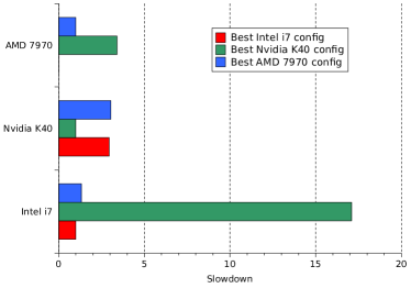
Figure 1: The slowdown of three different configurations compared to the best configuration for the different devices.

As we can see, using the ”wrong” configuration can seriously degrade the performance, even when that configuration is the best one for another device. For instance, using the best Nvidia configuration on the Intel i7 resulted in a slowdown of 17.1 compared to the best Intel configuration. Even between the two GPUs, which have a more similar architecture, the problem persisted. Using the best AMD configuration on the Nvidia card, or the best Nvidia configuration on the AMD card both resulted in slowdowns of approximately 3.

This clearly demonstrates the need for re-tuning OpenCL code when executing it on a new device. Furthermore, resorting to exhaustive search, as we did here, is in general not practical or even possible since the configurations spaces can be very large.

3 Related Work

Auto-tuning is a well established technique, which has been successfully applied in a number of widely used high performance libraries, such as FFTW[2, 3] for fast Fourier transforms, OSKI[4] for sparse matrices and ATLAS[5] for linear algebra[6].

There are also been examples of application specific empirical auto tuning on GPUs, e.g. for stencil computations [7], matrix multiplication [8] and FFTs [9]. Furthermore, analytical performance models for GPUs and heterogeneous systems have been developed[10, 11, 12, 13] and used for auto-tuning [14].

Much work has been done on machine learning based auto-tuning, e.g. to determine loop unroll factors[15], whether to perform SIMD vectorization[16] and general compiler optimizations [17]. Kulkarni et al.[18] developed a method to determine a good ordering of the compiler optimization phases, on a per function basis. Their method uses a neural network to determine the best optimization phase to apply next, given characteristics of the current, partially optimized code. They evaluated their method in a dynamic compilation setting, using Java. Singh et al. [19] used a method similar to ours, where they trained an artificial neural network performance model. However, they focus on large-scale parallel platforms such as the BlueGene/L, and do not use their model as part of a auto-tuner. Yigitbasi et al. [20] also adopt a similar approach to us, by building a machine learning based performance model for MapReduce with Hadoop, and using it in an auto-tuner. In contrast to these works, our method uses values of tuning parameters to directly predict execution time, as part of an auto-tuner, using OpenCL in a heterogeneous setting.

Machine learning approaches have also been used for auto-tuning applications in a heterogeneous setting. A number of works deals with developing methods to determine whether to execute a kernel on the GPU or CPU[21, 22] and to balance load between the devices[23, 24]. Magni et al. [25] used an ANN model to determine the correct thread coarsening factor, that is, the amount of work per thread, based on static code features, for OpenCL on different platforms. In another study, they use a nearest neighbor approach to determine the best way to parallelize sequential loops for OpenACC[26]. A method to determine whether local memory should be used as an optimization for OpenCL is proposed in [27]. A random forest based model is trained using millions of synthetic benchmarks, and based on manually extracted features of the memory access pattern predicts the speedup if local memory is used. Liu et al. [28] focus on how the properties of the program inputs affect the performance of CUDA programs, and develop a method where a machine learning based algorithm can be used to determine the best optimization parameters based on the input. In contrast to these works, we develop a performance model that predicts the execution time based on multiple different tuning parameters, and use it in a auto-tuner.

The two works most closely related to ours are [29, 30]. In [29], a model based on boosted regression trees were used to build an auto-tuner, evaluated with a single GPU benchmark, filterbank correlation. The Starchart [30] system builds a regression tree model which can be used to partition the design space, discover its structure and find optimal parameter values within the different regions. It is then used to develop an auto-tuner for several GPU benchmarks. In contrast, our work uses a different machine learning model, has more parameters for each kernel, and uses OpenCL to tune applications for both CPUs and GPUs.

Work has also been done on OpenCL performance portability. Zhang et al. [31] identify a number of parameters, or tuning knobs, which affects the performance of OpenCL codes on different platforms, and shows how setting the appropriate values can improve performance. Faberio et al. [32] use iterative optimization to adapt OpenCL kernels to different hardware by picking the optimal tiling sizes. Pennycook et al.[33] take a different approach, and attempt to determine application settings which will achieve good performance on different devices, rather than optimal performance on any single device.

4 Background

One of the currently most popular heterogeneous platforms is the combination of a CPU and a GPU. While GPUs traditionally were developed for rendering graphics, they have evolved into general purpose programmable, highly parallel accelerators. Here we will only present a brief overview, for details on GPU architecture and applications, the reader is referred to [34, 35], and [36], which include a discussion of OpenCL on AMD and Nvidia GPUs.

GPUs consists of a number of compute units, each of which consists of several processing elements. The processing elements of a compute unit work in a SIMD fashion, executing instructions in lock step. The largest memory space available is global memory, which resides in slow, off-chip DRAM (but is separate from the system’s main memory). While the global memory is cached on newer GPUs, they also have a fast, on-chip, scratch pad memory, which can be used as a user managed cache. In addition, they have texture memory, which is optimized for access patterns with 2D and 3D spatial locality, and constant memory designed to allow for high performance when accessed by many threads concurrently.

4.1 OpenCL

OpenCL[1] is a standard for heterogeneous computing, which makes it possible to write code once, and execute it on different devices, including CPUs and GPUs. The code is organized into host code and kernels. The host code executes as a normal CPU program, and sets up and launches the kernels on a device (which might be the same CPU the host code is executing on). Kernels are executed in parallel by a number of threads known as work items, which are organized into work groups. If executed on a GPU, the work groups are typically mapped to compute units, and the work items to processing elements, on the CPU they are mapped to the CPU cores. A number of logical memory spaces exists: local memory (mapped to the fast on-chip memory on GPUs), image memory (mapped to the GPU texture memory), and constant memory (mapped to the hardware constant memory on the GPU). On the CPU, all of these memory spaces are typically mapped to main memory.

4.2 Machine Learning

This section will provide a basic introduction to machine learning with a focus on artificial neural networks, more details can be found in e.g. [37]. Machine learning algorithms can be broadly divided into unsupervised and supervised learning. In unsupervised learning, no output labels are given for the input, instead, the algorithm attempts to discover structure in the input data itself. In supervised learning on the other hand, the algorithm is given example input and output pairs, which are used to build a model which can later predict the output for unseen input. If the outputs are categories, this is known as classification, if they are real numbers, as regression. In both cases it can be viewed as form of function approximation.

Artificial neural networks are a supervised machine learning algorithm which can be used for both classification and regression. They are built up of artificial neurons, which have multiple inputs and a single output. The output of a neuron is found by first computing a weighed sum of the inputs, and then passing the result to an activation function, such as the sigmoid or threshold function. A neural network can be built by connecting the inputs and outputs of multiple neurons. Some neurons have unconnected inputs, these are the input neurons, while others have unconnected outputs, these are the output neurons. By presenting values to the input nodes, the network can compute the output by letting the values propagate through the network. A complete network, and a detailed view a single neuron, is shown in Figure 2.

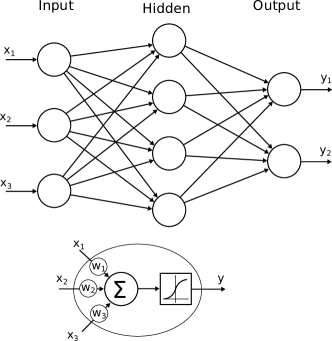
Figure 2: Neural network with 3 input neurons, a single hidden layer with 4 neurons, and two output neurons. Bellow, a single neuron with three inputs.

The weights of the neurons determine what the network computes and must be fitted to the example data, a process known as training. Several training algorithms exists, they all initialize the weights to random values, and attempt to adjust them so that the values computed by the network for the example inputs matches the example outputs.

The topology and activation function used in a network must be adjusted manually to the problem at hand. These factors can greatly affect the performance of the network, but little knowledge about how to pick values exists, and experimentation is often required.

5 Machine Learning based auto-tuning

Figure 3 illustrates our auto-tuning method. We start with parameterized benchmarks. The parameters form a space of possible implementations, and from this space we pick samples which are used to build the machine learning based model. The model is then used to predict the execution time for all the possible configurations. In a second stage, the $M$ configurations with the lowest predicted execution times are found, and their actual execution times are measured. The best of these configurations is then found, and returned by the auto-tuner. If the model is sufficiently accurate, the optimal configuration will be among those found in the second stage, and therefore returned by the auto-tuner.

Figure 3: Overview of our auto-tuning approach. Execution times for a random set of configurations are measured, and used to build a model, which is then used to pick interesting configurations for exhaustive search.

In the following we will cover these steps in more detail.

5.1 Code parameterization and Candidate Generation

We used three benchmarks for our experiments, convolution, raycasting and stereo, described in Table 1. The code of the benchmarks were parameterized with tuning parameters, to make it possible to generate multiple candidate implementations, with one candidate for each tuning parameter configuration. These candidates are all functionally equivalent, but the different values of the tuning parameters causes their performance to vary.

The tuning parameters determine whether or not various optimizations are applied, as well as the value of performance critical variables. Examples include whether or not to manually cache values in local memory, how much work should be assigned to each thread, and whether or not to perform loop unrolling. An overview and description of all the tuning parameters used, and their possible values, can be found in Table 2.

The optimal values for the parameters depends on the device being used, and possibly the input to the algorithm. Furthermore, since the parameters are not independent, the best values cannot be found by varying the values of one parameter at a time. As can be seen from Table 1, the size of the parameter spaces for are 131K, 655K and 2359K for convolution, raycasting and stereo respectively.

The parameters are implemented either using preprocessor macros in the kernel code, or using variables set on the host prior to kernel launch. The loop unrolling in convolution and stereo is implemented using OpenCL driver pragmas, while in raycasting, it is done manually, using preprocessor macros. Several of the parameters deal with storing data structures in different memory spaces. These parameters can in general be combined in any way, for instance, if both image and local memory is used, the data structure will first be stored in image memory, and then be manually cached in local memory.

Table 1: Benchmarks used

Benchmark	Description
convolution	convolution of 2048x2048 2D image with 5x5 box filter, example of stencil computation.
raycasting	Volume visualization generating 1024x1024 2D image from 512x512x512 3D volume data.
stereo	Computing disparity between two 1024x1024 stereo images to determine distances to objects.

Table 2: Parameters used for the benchmarks and their possible values. The parameters listed under all are present in all the benchmarks.

all
Parameter	Possible values
Work-group size in x dimension	1,2,4,8,16,32,64,128
Work-group size in y dimension	1,2,4,8,16,32,64,128
Output pixels per thread in x dimension	1,2,4,8,16,32,64,128
Output pixels per thread in y dimension	1,2,4,8,16,32,64,128
convolution
Parameter	Range
Use image memory	0,1
Use local memory	0,1
Add padding to image	0,1
Interleaved memory reads	0,1
Unroll loops	0,1
raycasting
Parameter	Possible values
Use image memory for data	0,1
Use image memory for transfer function	0,1
Use local memory for transfer function	0,1
Use constant memory for transfer function	0,1
Interleaved memory reads	0,1
Unroll factor for ray traversal loop	1,2,4,8,16
stereo
Parameter	Possible values
Use image memory for left image	0,1
Use image memory for right image	0,1
Use local memory for left image	0,1
Use local memory for right image	0,1
Unroll factor for disparity loop	1,2,4,8
Unroll factor for difference loop in x direction	1,2,4
Unroll factor for difference loop in x direction	1,2,4

5.2 Model building

The model we build should be able to predict the execution time of a benchmark given the tuning parameter configuration. To do this, we run the benchmarks on several randomly chosen parameter configurations and record the execution time. These input-output pairs, or training samples, are then used to build, or train, a model. Using machine learning terminology, this is known as supervised learning.

Multiple supervised learning algorithms exist. We have used artificial neural networks (ANN) due to their good predictive power, ability to handle arbitrary functions, and ability to handle noisy input robustly. A significant drawback of ANNs is, however, the opaqueness of the resulting model, which makes it difficult to interpret, and hard to gain deeper insights into how the different parameters interact, and contribute to the final performance.

Through experimentation, we found that a network with a single hidden layer with 30 neurons using sigmoid activation functions gave good performance.

Additionally, we used a technique know as bagging[38] to further increase the performance of the model. Rather than using all the training data to build a single neural network, we split it into $k$ parts and build $k$ networks, each trained using all the data except one of the parts. During prediction, we feed the input to all the networks, and then take the mean of their outputs as the final output. We found that this increased the accuracy of the predictions. We have used a value of 11 for $k$.

During ANN training, the weights are adjusted to minimize the mean squared error between the predictions and the actual output. In our case, this causes problems since we use the ANN to predict the execution time directly, and are therefore interested in minimizing the relative, rather than the absolute error. To resolve this problem, we take the logarithm of the execution times before training the neural network. The neural network then predicts the logarithm of the execution time, and attempts to minimize the mean squared error when comparing with the logarithm of the actual execution time. This works since reducing the absolute error of the logarithm of two values is equivalent to reducing the relative error of the values directly.

A challenge specific for this kind of data is invalid parameter configurations, that is, configurations for which the corresponding code cannot be run. This is typically because the resulting code uses too many resources, for instance, some devices places restrictions on how large work-groups can be, or how much local memory is available. If the specific device is known, most of the invalid configurations can be determined statically, but in some cases it is necessary to attempt to compile and run the kernels. We deal with this issue by simply ignoring these configurations when training the model.

5.3 Prediction and Evaluation

After the model is built, the optimal parameter configuration may be found by simply predicting the execution time for all possible configurations, and picking the best one. This remains feasible despite large parameter spaces since it is orders of magnitude faster to evaluate the model than to execute the actual benchmarks.

However, since the model is not perfectly accurate, it is unlikely that the configuration with the lowest predicted execution time is the one with the lowest actual execution time. Our auto-tuner therefore includes a second stage where the model to find interesting subspaces of the parameter space which are small enough to be searched exhaustively, and are likely to contain the actual optimal configurations.

In practice, we do this by picking the $M$ configurations with the lowest predicted execution times. We then measure the actual execution times of these configurations, and find the best among them. Again, this is not guaranteed to be the globally best configuration since the model may be so inaccurate that the globally optimal configuration is not included among the $M$ configurations in the second stage. Sometimes these $M$ configurations also include invalid configurations. This is, however, not a big problem if the models are trained with enough data.

Our experiments used values for $M$ in the range 10 - 200, with good results. However, by making assumptions about the distribution of the execution times, as well as the distribution of prediction errors this ad-hoc method could be replaced with a more principled one where one could determine values for $M$ so that the samples in the second stage contains the optimal one with a given probability.

6 Results

To evaluate our method, we implemented 3 parameterized benchmarks in OpenCL, stereo, convolution and raycasting, see Table 1. Descriptions of the parameters for all the benchmarks can be found in Table 2. For the experiments, we used an Nvidia K40 GPU, an AMD Radeon HD 7970 GPU and an Intel i7 3770 CPU.

The time required to train the ANN models is significant, but small compared to the cost of gathering the training data. For example, for the convolution benchmark on the Nvidia GPU, training the model with 2000 samples takes about 1 minute, gathering the data takes about 30 minutes. The time required to gather data is so high because it does not only include the time for the kernels themselves, but also the overhead of compiling the kernels, as well as time wasted attempting to compile and launch kernels with invalid configurations.

To evaluate the accuracy of the models created, we compared the predictions against actual execution times for valid parameter configurations not used during training. This was repeated for neural networks trained using an increasing number of configurations. Since the output of the model depends on the particular configurations used during training, as well as the random initial weights of the neural network, we built several neural networks using different configurations for each training size and report the mean of the output for all these networks. The results are shown in figures 4, 5 and 6 for the Nvidia, Intel and AMD devices respectively.

As is shown, the mean relative error decreases as more samples are used to train the models, but stabilizes or decreases much more slowly after around 1000-2000 samples, for all devices and benchmarks. The accuracy on the Intel CPU is noticeably better than for the GPUs, the relative mean accuracy is 6.1% - 8.3% for 4000 training configurations on the CPU, the corresponding numbers are 12.5%-14.7% and 12.6%-21.2% for the Nvidia and AMD GPUs respectively. The performance of the different benchmarks is relatively similar on the Intel CPU and Nvidia GPU, on the AMD, raycasting performs significantly better than convolution and stereo.

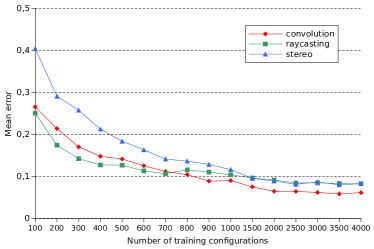
Figure 4: Mean prediction error for the different benchmarks for increasing number of training samples, on the Intel i7.

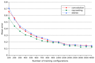
Figure 5: Mean prediction error for the different benchmarks for increasing number of training samples, on the Nvidia K40.

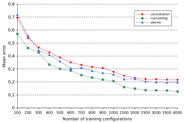
Figure 6: Mean prediction error for the different benchmarks for increasing number of training samples, on the AMD 7970.

We also investigated the performance on different devices from the same vendor, Figure 7 shows accuracy for the convolution benchmark for three different Nvidia GPUs, a C2070, a K40 and a GTX980, representing the Fermi, Kepler and Maxwell architectures respectively. As the figure shows, the accuracy is similar for the K40 and c2070, while slightly worse for the GTX980.

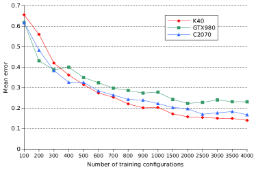
Figure 7: Mean prediction error for convolution on different Nvidia GPUs.

Another way to visualize the accuracy is to scatter plot the actual versus the predicted execution times. This is done for the convolution benchmark in figures 9, 8 and 10, for the Nvidia, Intel and AMD devices, respectively. The figures show 100 configurations not used during training. In this case, the results are not the average of multiple models. As the figures show, there is a good match between predictions and reality. The clustering of the Intel data is caused by the values of the local and image memory parameters. Here, using image memory without local memory results in a significantly worse performance compared to all other combinations of these parameter values.

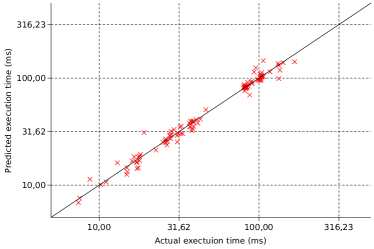
Figure 8: Predicted versus actual execution times, on the Intel i7. Note the logarithmic scales.

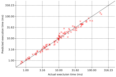
Figure 9: Predicted versus actual execution times, on the Nvidia K40. Note the logarithmic scales.

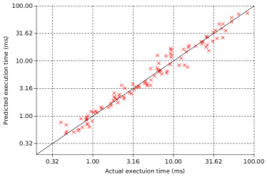
Figure 10: Predicted versus actual execution times, on the AMD 7970. Note the logarithmic scales.

For the convolution benchmark, the parameter space is fairly small compared to the two other benchmarks, and it was therefore possible to measure the actual execution times of all possible configurations. This allows us to evaluate our auto-tuners ability to find good configurations, since we can compare against the known globally optimal configuration.

In figures 11, 12 and 13 we have varied both the number of configurations used for training the model, and the number $M$ of configurations used in the second stage of our auto-tuner. We expect best results when both of these are high. As above, we built several networks for each combination, and report the mean of the results. Some results are missing, due to a high number of invalid configurations being predicted.

As can be seen, out auto-tuner is able to find good configurations. E.g. when we use 2000 configurations in the first stage, and 200 in the second stage, we are able to find configurations which on average are 3.5%, 5.8% and 8.7% slower than the global optimum, for the Intel, AMD and Nvidia devices, respectively, after evaluating only 1.7% of the possible configurations. In some cases, we are even able to find the global optimums, but poorer results in other cases pull the averages down. When fewer configurations are used, the results are worse, when 500 configurations are used in the first stage, and 100 in the second, we find solutions on average 13.0%, 29.3% and 29.7% slower than the optimum for the Intel, AMD and Nvidia devices, respectively.

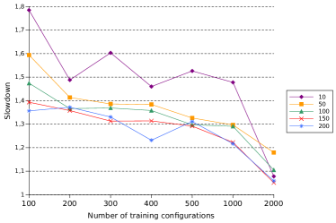
Figure 11: Average slowdown of results from our auto-tuner compared to the globally optimal solution, Nvidia K40.

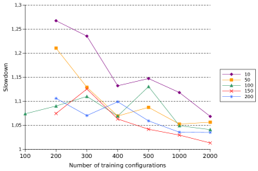
Figure 12: Average slowdown of results from our auto-tuner compared to the globally optimal solution, on the Intel i7. Some results missing due to invalid configurations.

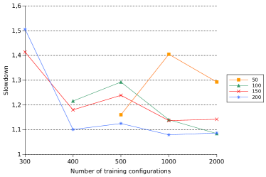
Figure 13: Average slowdown of results from our auto-tuner compared to the globally optimal solution, on the AMD 7970. Some results missing due to invalid configurations.

For the stereo and raycasting benchmarks, the parameter spaces are so large that time constrains prevented us from exhaustively evaluating all configurations. The best parameter configurations are therefore not known, making performance evaluation harder. We have, however, measured the execution time of 50K random configurations for both benchmarks, and compared the best output found to the output of our auto-tuner. The results are shown in Figure 14, here we have used 3000 configurations in the first stage, and 300 configurations in the second stage. This corresponds to 0.5% and 0.1% of the configurations spaces for raycasting and stereo, respectively. As the figure shows, we are able to find good configurations, in some cases slightly better than the best among the 50K random samples. We would like to reemphasize that these are only preliminary results, since we don’t know the truly best configuration. Since the model predicted mostly invalid configurations for the stereo benchmark on the GPUs, we do not report any results for these cases.

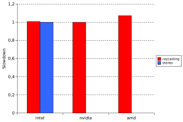
Figure 14: Average slowdown of results from auto-tuner compared to the globally optimal solution, for various values of $N$ and $M$, on the AMD 7970. Some results missing due to invalid configurations.

7 Further Discussions

First there is the issue of the varying accuracy achieved for the different devices. In particular, the mean relative error for the Intel CPU is between 6.1% and 8.3%, while the corresponding numbers are 12.5%-14.7% and 12.6%-21.2% for the Nvidia and AMD GPUs respectively. One possible explanation is that the memory related parameters may have less effect on the CPU than the GPUs, since all the logical memory spaces are mapped to the same physical memory on the CPU, as described in Section 4. An exception here is the effect which causes the clustering of the convolution data, as described in Section 6. This effect is not present in the other benchmarks, and may be the reason why convolution has best accuracy.Furthermore, there are fewer invalid configurations on the CPU, which increases the accuracy. Finally, while the problem sizes has been adjusted to partly compensate for this, the execution times on the CPU are generally longer, potentially making the timing measurements more reliable.

Secondly, there is the issue of the varying performance for the different benchmarks on the AMD GPU. On both the Intel and Nvidia devices, the performance for the different benchmarks are fairly equal. However, on the AMD GPU, raycasting performs significantly better than stereo and convolution. This may be related to how the AMD OpenCL driver performs loop unrolling. As described in Section 5, the loop unrolling in raycasting is done manually, with macros, while the unrolling in the two other benchmarks relies on the OpenCL driver, which may be more unreliable.

Finally the current method of simply ignoring invalid configurations during model training have as a consequence that the model have poor accuracy in the invalid parameter configuration subspaces. This can cause the model to predict that invalid configurations have low execution times. In some cases, all the configurations in the second stage can be invalid, the net effect of which is that the auto-tuner gives no prediction at all. This can be seen in several of out results, and a better scheme to deal with this should be developed to improve performance.

8 Conclusion and Future Work

We have developed and validated a machine learning based auto-tuning framework for OpenCL. The framework measures the performance of several candidate implementations from a parameter configuration space and uses this result to build a artificial neural network, which works as a performance model. This model is then used to find interesting parts of the configuration space, which are explored exhaustively to find good candidate implementations. Our neural network model achieves a mean relative error as low as 6.1% for three different benchmarks executed on three different devices, a Intel i7 3770 CPU, an Nvidia K40 GPU and a AMD Radeon HD 7970. The autotuner is able to find good configurations, at best only 1.3% slower than the best configuration.

Future work includes enhancing the performance of the model, in particular with regard to invalid configurations, evaluating the model on novel hardware architectures, beyond just CPUs and GPUs, and integrating problem parameters into the performance model. Incorporating advanced new features specific to a given architecture[39] will remain challenging. However, studying multi-GPU systems[40] and looking into multi-variate analysis[41] may also be interesting avenues of inquiry.

9 Acknowledgements

The authors would like to thank Nvidia’s CUDA Research Center program, and NTNU for hardware donations, and Malik Khan for helpful discussions.

References

- [1] KHRONOS Group, OpenCL - The open standard for parallel programming of hetrogeneous systems, 2015. http://www.khronos.org/opencl/ Acessed 15.01.2015.
- [2] M. Frigo and S. G. Johnson, “The design and implementation of FFTW3,” Proceedings of the IEEE, vol. 93, no. 2, pp. 216–231, 2005. Special issue on “Program Generation, Optimization, and Platform Adaptation”.
- [3] A. Elster and J. Meyer, “A super-efficient adaptable bit-reversal algorithm for multithreaded architectures,” in Parallel Distributed Processing, 2009. IPDPS 2009. IEEE International Symposium on, pp. 1–8, May 2009.
- [4] R. Vuduc, J. W. Demmel, and K. A. Yelick, “Oski: A library of automatically tuned sparse matrix kernels,” Journal of Physics: Conference Series, vol. 16, no. 1, p. 521, 2005.
- [5] R. C. Whaley and A. Petitet, “Minimizing development and maintenance costs in supporting persistently optimized BLAS,” Software: Practice and Experience, vol. 35, pp. 101–121, February 2005.
- [6] R. E. Jensen, I. Karlin, and A. C. Elster, “Auto-tuning a matrix routine for high performance,” Norsk informatikkonferanse, vol. 2011, 2011.
- [7] Y. Zhang and F. Mueller, “Auto-generation and auto-tuning of 3D stencil codes on GPU clusters,” in Proceedings of the Tenth International Symposium on Code Generation and Optimization, CGO ’12, (New York, NY, USA), pp. 155–164, ACM, 2012.
- [8] Y. Li, J. Dongarra, and S. Tomov, “A note on auto-tuning GEMM for GPUs,” in Proceedings of the 9th International Conference on Computational Science: Part I, ICCS ’09, (Berlin, Heidelberg), pp. 884–892, Springer-Verlag, 2009.
- [9] A. Nukada and S. Matsuoka, “Auto-tuning 3-D FFT library for CUDA GPUs,” in Proceedings of the Conference on High Performance Computing Networking, Storage and Analysis, SC ’09, (New York, NY, USA), pp. 30:1–30:10, ACM, 2009.
- [10] J. C. Meyer, Perfromance Modeling of Heterogeneous Systems. PhD thesis, Norwegian University of Science and Technology, 2012.
- [11] J. Meyer and A. Elster, “Performance modeling of heterogeneous systems,” in Parallel Distributed Processing, Workshops and Phd Forum (IPDPSW), 2010 IEEE International Symposium on, pp. 1–4, April 2010.
- [12] J. C. Meyer and A. C. Elster, “BSP as a performance predictor on heterogeneous interconnect platforms,” in Proceedings of 9th Intl. Workshop on State of the Art in Scientific Computing (PARA 2008), Springer LNCS, 2008.
- [13] S. Hong and H. Kim, “An analytical model for a GPU architecture with memory-level and thread-level parallelism awareness,” in ACM SIGARCH Computer Architecture News, vol. 37, pp. 152–163, ACM, 2009.
- [14] K. Yotov et al., “A comparison of empirical and model-driven optimization,” SIGPLAN Not., vol. 38, pp. 63–76, May 2003.
- [15] M. Stephenson and S. Amarasinghe, “Predicting unroll factors using supervised classification,” in Code Generation and Optimization, 2005. CGO 2005. International Symposium on, pp. 123–134, IEEE, 2005.
- [16] A. Trouvé et al., “Predicting vectorization profitability using binary classification,” IEICE TRANSACTIONS on Information and Systems, vol. 97, no. 12, pp. 3124–3132, 2014.
- [17] G. Fursin et al., “Milepost GCC: Machine learning enabled self-tuning compiler,” International journal of parallel programming, vol. 39, no. 3, pp. 296–327, 2011.
- [18] S. Kulkarni and J. Cavazos, “Mitigating the compiler optimization phase-ordering problem using machine learning,” in Proceedings of the ACM International Conference on Object Oriented Programming Systems Languages and Applications, OOPSLA ’12, (New York, NY, USA), pp. 147–162, ACM, 2012.
- [19] K. Singh et al., “Predicting parallel application performance via machine learning approaches,” Concurrency and Computation: Practice and Experience, vol. 19, no. 17, pp. 2219–2235, 2007.
- [20] N. Yigitbasi et al., “Towards machine learning-based auto-tuning of mapreduce,” in Modeling, Analysis Simulation of Computer and Telecommunication Systems (MASCOTS), 2013 IEEE 21st International Symposium on, pp. 11–20, Aug 2013.
- [21] W. F. Ogilvie et al., “Active learning accelerated automatic heuristic construction for parallel program mapping,” in Proceedings of the 23rd International Conference on Parallel Architectures and Compilation, PACT ’14, pp. 481–482, ACM, 2014.
- [22] D. Grewe, Z. Wang, and M. O’Boyle, “Portable mapping of data parallel programs to OpenCL for heterogeneous systems,” in Code Generation and Optimization (CGO), 2013 IEEE/ACM International Symposium on, pp. 1–10, Feb 2013.
- [23] I. Grasso et al., “Automatic problem size sensitive task partitioning on heterogeneous parallel systems,” SIGPLAN Not., vol. 48, pp. 281–282, Feb. 2013.
- [24] J. Li et al., “Machine learning based online performance prediction for runtime parallelization and task scheduling,” in Performance Analysis of Systems and Software, 2009. ISPASS 2009. IEEE International Symposium on, pp. 89–100, April 2009.
- [25] A. Magni, C. Dubach, and M. O’Boyle, “Automatic optimization of thread-coarsening for graphics processors,” in Proceedings of the 23rd International Conference on Parallel Architectures and Compilation, PACT ’14, (New York, NY, USA), pp. 455–466, ACM, 2014.
- [26] A. Magni, D. Grewe, and N. Johnson, “Input-aware auto-tuning for directive-based GPU programming,” in Proceedings of the 6th Workshop on General Purpose Processor Using Graphics Processing Units, GPGPU-6, (New York, NY, USA), pp. 66–75, ACM, 2013.
- [27] T. D. Han and T. S. Abdelrahman, “Automatic tuning of local memory use on GPGPUs,” arXiv preprint arXiv:1412.6986, 2014.
- [28] Y. Liu, E. Zhang, and X. Shen, “A cross-input adaptive framework for GPU program optimizations,” in Parallel Distributed Processing, 2009. IPDPS 2009. IEEE International Symposium on, pp. 1–10, May 2009.
- [29] J. Bergstra, N. Pinto, and D. Cox, “Machine learning for predictive auto-tuning with boosted regression trees,” in Innovative Parallel Computing (InPar), 2012, pp. 1–9, May 2012.
- [30] W. Jia, K. A. Shaw, and M. Martonosi, “Starchart: Hardware and software optimization using recursive partitioning regression trees,” in Proceedings of the 22Nd International Conference on Parallel Architectures and Compilation Techniques, PACT ’13, pp. 257–268, IEEE Press, 2013.
- [31] Y. Zhang, I. Sinclair, Mark, and A. Chien, “Improving performance portability in OpenCL programs,” in Supercomputing (J. Kunkel, T. Ludwig, and H. Meuer, eds.), vol. 7905 of Lecture Notes in Computer Science, pp. 136–150, Springer Berlin Heidelberg, 2013.
- [32] J. F. Fabeiro, D. Andrade, and B. B. Fraguela, “OCLoptimizer: An iterative optimization tool for OpenCL,” Procedia Computer Science, vol. 18, no. 0, pp. 1322 – 1331, 2013. 2013 International Conference on Computational Science.
- [33] S. Pennycook et al., “An investigation of the performance portability of OpenCL,” Journal of Parallel and Distributed Computing, vol. 73, no. 11, pp. 1439 – 1450, 2013. Novel architectures for high-performance computing.
- [34] J. Owens and J. others, “GPU computing,” Proceedings of the IEEE, vol. 96, pp. 879–899, May 2008.
- [35] A. R. Brodtkorb, C. Dyken, T. R. Hagen, J. M. Hjelmervik, and O. O. Storaasli, “State-of-the-art in heterogeneous computing,” Scientific Programming, vol. 18, no. 1, pp. 1–33, 2010.
- [36] E. Smistad, T. L. Falch, M. Bozorgi, A. C. Elster, and F. Lindseth, “Medical image segmentation on gpus–a comprehensive review,” Medical Image Analysis, vol. 20, no. 1, pp. 1–18, 2015.
- [37] T. Hastie, R. Tibshirani, and J. Friedman, The elements of statistical learning : data mining, inference, and prediction. Springer Science + Business Media, 2009.
- [38] Z.-H. Zhou, J. Wu, and W. Tang, “Ensembling neural networks: Many could be better than all,” Artificial Intelligence, vol. 137, no. 1–2, pp. 239 – 263, 2002.
- [39] T. L. Falch and A. C. Elster, “Register caching for stencil computations on GPUs,” in Symbolic and Numeric Algorithms for Scientific Computing (SYNASC), 2014 16th International Symposium on, pp. 479–486, IEEE, 2014.
- [40] D. G. Spampinato, A. C. Elster, and T. Natvig, “Modelling multi-GPU systems.,” in Parallel Computing: From Multicores and GPU’s to Petascale, vol. 19, pp. 562–569, IO Press, 2010.
- [41] H. Martens and M. Martens, Multivariate analysis of quality: an introduction. John Wiley & Sons, 2001.