Exact Error Analysis and Energy-Efficiency Optimization of Regenerative Relay Systems with Spatial Correlation

Abstract

Energy efficiency and its optimization constitute critical tasks in the design of low-power wireless networks. The present work is devoted to the error rate analysis and energy-efficiency optimization of regenerative cooperative networks in the presence of multipath fading under spatial correlation. To this end, exact and asymptotic analytic expressions are firstly derived for the symbol-error-rate of $M{-}$ary quadrature amplitude and $M{-}$ary phase shift keying modulations assuming a dual-hop decode-and-forward relay system, spatially correlated Nakagami${-}m$ multipath fading and maximum ratio combining. The derived expressions are subsequently employed in quantifying the energy consumption of the considered system, incorporating both transmit energy and the energy consumed by the transceiver circuits, as well as in deriving the optimal power allocation formulation for minimizing energy consumption under certain quality-of-service requirements. A relatively harsh path-loss model, that also accounts for realistic device-to-device communications, is adopted in numerical evaluations and various useful insights are provided for the design of future low-energy wireless networks deployments. Indicatively, it is shown that depending on the degree of spatial correlation, severity of fading, transmission distance, relay location and power allocation strategy, target performance can be achieved with large overall energy reduction compared to direct transmission reference.

I Introduction

Emerging communication systems are expected to provide high-speed data transmission, efficient wireless access, high quality of service (QoS) and reliable network coverage with reduced processing time and energy as well as widespread use of smart phones and other intelligent mobile devices. However, the currently witnessed scarcity of the two core fundamental resources, power and bandwidth, constitutes a significant challenge to satisfy these demands while it is known that wireless channel impairments such as multipath fading, shadowing and interference degrade information signals during wireless propagation. Furthermore, most energy constrained devices, such as terminals of mobile cellular, ad-hoc and wireless sensor networks, are typically powered by small batteries where replacement is rather difficult and costly [1],[2]. Therefore, finding a robust strategy for energy efficient transmission and minimized energy consumption per successfully communicated information bit is essential in effective design and deployment of wireless systems. This accounts for example for cases such as low-energy sensor networks in ecological environment monitoring as well as energy consumption in infrastructure devices of cellular systems. In addition, it is in line with global policies and strategies on low energy consumption and awareness on environmental issues which, among others, has led to the rapid emerge of green communications [3],[4].

It has been shown that multi-antenna systems constitute an effective method that can enhance spectral efficiency. However, this typically comes at a cost of complex transceiver circuitry and in massive systems with high energy consumption requirements. Furthermore, it is not currently feasible to embody large multi-antenna systems at hand held terminals due to spatial restrictions. As a result, cooperative communications have been proposed as an alternative solution that improves coverage as well as performance under fading effects and have attracted significant attention due to their ability to overcome the limitations of resource constrained wireless access networks, see e.g. [8, 12, 17, 6, 10, 14, 16, 18, 5, 7, 9, 11, 13, 15] and the references therein. A distinct feature of cooperative communications is that wireless agents share resources, instead of competing for them, which ultimately enhances system performance. In this context, various resource allocation algorithms and techniques have been proposed for improving the energy efficiency of resource constrained wireless networks. Specifically, the authors in [19] analyzed energy-efficient direct transmission adopting higher-level modulation for short distances, where circuit power is more dominant than transmission power. It was also suggested that high energy reduction can be achieved by optimizing the transmission time and the modulation parameters, particularly for short transmission distances. The authors in [20] addressed the optimal power allocation and throughput transmission strategy for minimizing the total energy consumption required to transmit a given number of bits. In [21], minimization of two-hop transmission energy with joint relay selection and power control was proposed for two policies: i) for minimizing the energy consumption per data packet; ii) for maximizing the network lifetime. In the same context, [22, 23, 25, 26, 24] addressed the modulation optimization for minimizing the total energy consumption for $M{-}$ary quadrature amplitude modulation ($M{-}$QAM), whereas energy efficient cooperative communication in clustered sensor networks was investigated in [27]. Energy efficiency in cooperative networks was also analyzed in [32, 33, 34, 29, 30, 35, 28, 31] by optimizing energy consumption based on the involved relay decoding strategy, modulation parameters, number of relay nodes and their distance from the source and the destination nodes. Likewise, an energy-efficient scheme was proposed in [36] by exploiting the wireless broadcast nature and the node overhearing capability while an optimal energy efficient strategy based on the cooperative network parameters and transmission rate was reported in [37]. Finally, the authors in [38] analyzed realistic scenarios of energy efficient infrastructure-to-vehicle communications.

It is also widely known that fading phenomena constitute a crucial factor of performance degradation in conventional and emerging wireless communication systems. Based on this, numerous investigations have addressed the effect of different types of fading conditions on the performance of cooperative communications [41, 43, 45, 47, 50, 53, 55, 39, 40, 42, 44, 46, 49, 51, 52, 54, 48, 56]. However, the vast majority of the reported investigations assume that the involved communication paths are statistically independent to each-other. Nevertheless, this assumption is rather simplistic as in realistic cooperative communication scenarios the wireless channels may be spatially correlated, which should be taken into account particularly for deployments relating to low-energy consumption requirements. Based on this, the authors in [57] addressed the spatial correlation in relay communications over fading channels whereas the performance of a decode-and-forward (DF) system with $M{-}$PSK modulated signals in triple correlated branches over Nakagami${-}m$ fading channels using selection combining was investigated in [58]. In the same context, the authors in [59] analyzed the performance of a multiple-input-multiple-output (MIMO) DF system with orthogonal space time transmission over spatially correlated Nakagami${-}m$ fading channels for integer values of $m$. The performance of a two hop amplify and forward (AF) relay network with beamforming and spatial correlation for the case that the source and destination are equipped with multiple antennas while the relay is equipped with a single antenna was investigated in [60]. Likewise, spatial correlation in the context of indoor office environments and multi-antenna AF relaying with keyhole effects was analyzed in [61] and [62], respectively whereas the effects of spatial correlation on the performance of similar relaying systems were analyzed in [63, 64, 65, 66]. However, to the best of the authors knowledge, a comprehensive exact and asymptotic error rate analysis for regenerative systems over spatially correlated channels using maximum-ratio-combing (MRC) as well as a detailed energy-efficiency analysis and optimization, have not been reported in the open technical literature.

Motivated by the above, the aim of this work is twofold: we, firstly, derive exact analytic expressions for the SER of a two-hop DF relay system over spatially correlated Nakagami${-}m$ fading channels for both $M{-}$QAM and $M{-}$PSK constellations along with simple and accurate asymptotic expressions for high signal-to-noise ratio (SNR) values. Secondly, we provide a comprehensive analysis of energy-efficiency and the corresponding optimization in terms of power allocation between cooperating devices. This is realized by minimizing the average total energy consumption of the DF relay network over multipath fading conditions, for a given destination bit error rate (BER) and maximum transmit power constraints.

In more details, the technical contributions of the present article are outlined below:

• Exact closed-form expressions are derived for the end-to-end SER of $M{-}$QAM and $M{-}$PSK based dual-hop regenerative relay networks with MRC reception at the destination over Nakagami${-}m$ multipath fading channels with arbitrary spatial correlation between source-destination (S-D) and relay-destination (R-D) links.

• Simple closed-form asymptotic expressions are derived for the above scenarios for high SNR values.

• The offered analytic results are employed in a comprehensive energy optimization analysis based on minimizing the average total energy consumption of the overall regenerative relay network under a given QoS target, in terms of bit-error-rate (BER), and maximum transmit power constraints.

The remainder of this paper is organized as follows: Section II presents the considered relay system and channel model while Sections III and IV are devoted to the derivation of the corresponding exact and asymptotic error rate results. The total power consumption models are presented in Section V while the analysis of energy minimization and power allocation optimization based on the given constraints are provided in Section VI. Section VII presents the corresponding numerical results along with extensive analysis and discussions while closing remarks are provided in Section VIII.

II System and Channel Model

We consider a two-hop cooperative radio access system model consisting of source node (S), a relay node (R) and a destination node (D), where each node is equipped with a single antenna, as illustrated in Fig. 1. Without loss of generality, the system can represent both a conventional and emerging communication scenarios such as, for example, a mobile ad-hoc network or a vehicle-to-vehicle communication system. The cooperative strategy is based on a half-duplex DF relaying where transmission is performed using time division multiplexing. It is also assumed that the destination is equipped with MRC reception and that information signals are subject to multipath fading conditions that follow the Nakagami${-}m$ distribution.

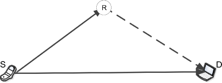
Figure 1: A dual-hop cooperative single relay model.

In phase I, the source broadcasts the signal to both destination and relay nodes and the corresponding received signals can be expressed as

$$y_{S,D}=\sqrt{\frac{P_{S}}{P_{L_{S,D}}}}h_{S,D}x+n_{S,D}$$ (1)

and

$$y_{S,R}=\sqrt{\frac{P_{S}}{P_{L_{S,R}}}}h_{S,R}x+n_{S,R}$$ (2)

respectively, where $P_{S}$ is the transmit power, $x$ is the transmitted symbol with normalized unit energy in the first transmission phase and $P_{L_{S,D}}$ and $P_{L_{S,R}}$ denote the path loss values in the S-D and source-relay (S-R) paths, respectively. Also, $h_{S,D}$ and $h_{S,R}$ are the complex fading coefficients of the S-D and S-R wireless links, respectively, whereas $n_{S,D}$ and $n_{S,R}$ are the corresponding complex Gaussian noise terms with zero mean and variance $N_{0}$. The relay then checks whether the received signal can be decoded correctly, which can be, for example, realized by examining the included cyclic-redundancy-check (CRC) digits or the received SNR levels[55],[57]. Based on this, if the signal is successfully decoded, the relay forwards it to the destination during phase II with power $\overline{P}_{R}=P_{R}$; otherwise, the relay does not transmit and remains idle with $\overline{P}_{R}=0$. Hence, the signal at the destination during phase II can be represented as

$$y_{R,D}=\sqrt{\frac{\bar{P}_{R}}{P_{L_{R,D}}}}\>h_{R,D}x+n_{R,D}$$ (3)

where $\bar{P}_{R}$ is the transmit power of the relay, $P_{L_{R,D}}$ is the path loss of the R-D path and $h_{R,D}$ and $n_{R,D}$ denote the channel coefficient and complex Gaussian noise term with zero mean and variance $N_{0}$, respectively. Finally, the destination combines the received direct and relayed signals based on MRC principle where the combined SNR can be expressed as follows [57],[67]

$$\gamma_{\rm MRC}=\frac{(P_{S}/P_{L_{S,D}})\mid h_{S,D}\mid^{2}+(\bar{P}_{R}/P_{L_{R,D}})\mid h_{R,D}\mid^{2}}{N_{0}}$$ (4)

The fading between the devices is assumed to follow the Nakagami${-}m$ distribution, which is a widely used model as the fading parameter $m$ can easily account for both severe and moderate fading conditions. Thus, the corresponding channel power gains ${\mid h_{S,D}\mid}^{2}$,${\mid h_{S,R}\mid}^{2}$ and ${\mid h_{R,D}\mid}^{2}$ follow the gamma distribution [68] with different power parameters, $\frac{1}{\Omega_{S,D}}$,$\frac{1}{\Omega_{S,R}}$, $\frac{1}{\Omega_{R,D}}$, and fading parameters $m_{S,D}$, $m_{S,R}$ and $m_{R,D}$, respectively.

In the considered regenerative system, arbitrary spatial correlation is assumed to exist between the S-D and R-D paths, as also adopted in the semi-analytical contribution of [57]. To this effect, the corresponding MGF for the case of Nakagami$-m$ fading is expressed as [69]

$$M(s)=\left(1-\frac{(\overline{\gamma}_{S,D}/P_{L_{S,D}}+\overline{\gamma}_{R,D}/P_{L_{R,D}})}{m}s+\frac{(1-\rho)\overline{\gamma}_{S,D}\overline{\gamma}_{R,D}/(P_{L_{S,D}}P_{L_{R,D}})}{m^{2}}s^{2}\right)^{-m},\;s<0$$ (5)

where $\overline{\gamma}_{S,D}$ and $\overline{\gamma}_{R,D}$ are the corresponding average SNR values, $s$ denotes the MGF parameter and $\rho={\rm Cov}(|h_{S,D}|^{2},|h_{R,D}|^{2}){/}\sqrt{{\rm Var}(|h_{S,D}|^{2}){\rm Var}(|h_{R,D}|^{2})}$ represents the involved correlation coefficient [68, 69], with ${\rm Cov}(\cdot)$ and ${\rm Var}(\cdot)$ denoting covariance and variance operations, respectively. It is acknowledged that other practical impairments, such as co-channel interference, are not considered in this work.

III SER for $M-$QAM Modulation in Nakagami$-m$ Fading with Spatial Correlation

This section is devoted to the error probability analysis of the dual-hop cooperative network over Nakagami${-}m$ fading channels with spatial correlation between the direct and the relay-destination paths [68]. To this effect and assuming MRC reception, the average end-to-end SER can be expressed as [57]

$$\begin{split}\overline{\rm SER}^{C}_{D}=&F_{\rm QAM}\left[\frac{1}{\left(1+\frac{(P_{S}\>/P_{L_{S,D}})\,\Omega_{S,D}\,g_{QAM}}{N_{0}m_{c}\sin^{2}\theta}\right)^{m_{c}}}\right]F_{\rm QAM}\left[\frac{1}{\left(1+\frac{(P_{S}/\>P_{L_{S,R}})\,\Omega_{S,R}\,g_{\rm QAM}}{N_{0}m_{S,R}\sin^{2}\theta}\right)^{m_{S,R}}}\right]\\ &+F_{\rm QAM}\left[\frac{1}{\left(1+\frac{[(P_{S}\Omega_{S,D}/\>P_{L_{S,D}})+({P}_{R}\Omega_{R,D}/\>P_{L_{R,D}})]\>\>g_{QAM}}{N_{0}m_{c}\sin^{2}\theta}+\frac{(1-\rho)P_{S}{P}_{R}\Omega_{S,D}\Omega_{R,D}g^{2}_{\rm QAM}}{N_{0}^{2}P_{L_{S,D}}P_{L_{R,D}}m_{c}^{2}\sin^{4}\theta}\right)^{m_{c}}}\right]\\ &\quad\times\left\{1-F_{\rm QAM}\left[\frac{1}{\left(1+\frac{(P_{S}/\>P_{L_{S,R}})\,\>\Omega_{S,R}\>g_{QAM}}{N_{0}m_{S,R}\sin^{2}\theta}\right)^{m_{S,R}}}\right]\right\}\end{split}$$ (6)

where $m_{c}=m_{S,D}=m_{R,D}$, $g_{\rm QAM}={3}/{2(M-1)}$ and

$$F_{\rm QAM}\left[v(\theta)\right]=\frac{4}{\pi}\left(1-\frac{1}{\sqrt{M}}\right)\int_{0}^{\pi/2}v(\theta){\>{\rm d}\theta}-\frac{4}{\pi}\left(1-\frac{1}{\sqrt{M}}\right)^{2}\int_{0}^{\pi/4}v(\theta)\>{\rm d}\theta.$$ (7)

The first two terms in (6) refer to the cases of incorrect and correct decoding of the received signal at the relay node, respectively, whereas the integral representation in (7) is used for evaluating the $\overline{\rm SER}^{C}_{D}$ numerically. In what follows, we firstly derive a closed-form expression for the average SER in the case of direct communication mode. This expression is subsequently employed in the derivation of exact closed-form expressions for the average SER of $M-$QAM and $M-$PSK modulated regenerative systems over Nakagami$-m$ fading channels with spatial correlation. Furthermore, it is used in the analysis of the energy consumption model and energy minimization in Sec. VI as it allows the derivation of an accurate expression for the energy consumption in the direct transmission, which acts as a benchmark in the evaluation of the energy reduction of the cooperative system.

III-A Exact SER for the Direct Transmission (DT)

Theorem 1.

For $P_{S},P_{L_{S,D}},\Omega_{S,D},N_{0},g_{\rm QAM}\in\mathbb{R}^{+}$, $M\in\mathbb{N}$ and $m_{S,D}\geq\frac{1}{2}$, the symbol error rate of a $M{-}QAM$ direct transmission scheme can be expressed as follows,

$$\begin{split}\overline{\rm SER}^{D}_{D}&=\frac{2(\sqrt{M}-1)N_{0}^{m_{S,D}}m_{S,D}^{m_{S,D}}P_{L_{S,D}}}{\sqrt{\pi}M(m_{S,D}\,N_{0}P_{L_{S,D}}+P_{S}\Omega_{S,D}g_{\rm QAM})^{m_{S,D}}}\\ &\quad\times\left\{\frac{\Gamma\left(m_{S,D}+\frac{1}{2}\right)}{\Gamma(m+1)}\,_{2}F_{1}\left(m_{S,D},\frac{1}{2},m_{S,D}+1,\frac{m_{S,D}N_{0}P_{L_{S,D}}}{m_{S,D}N_{0}P_{L_{S,D}}+P_{S}\Omega_{S,D}g_{\rm QAM}}\right)\right.\\ &\left.\,\qquad\,+\frac{\sqrt{2}(\sqrt{M}-1)}{\sqrt{\pi}}F_{1}\left(\frac{1}{2},\frac{1}{2}-m_{S,D},m_{S,D},\frac{3}{2},\frac{1}{2},\frac{m_{S,D}N_{0}P_{L_{S,D}}}{2(m_{S,D}N_{0}P_{L_{S,D}}+P_{S}\Omega_{S,D}g_{\rm QAM})}\right)\right\}\end{split}$$ (8)

where $\,{}_{2}F_{1}(.)$ and $F_{1}(.)$ denote the Gauss hypergeometric function and the Appell hypergeometric function of the first kind, respectively.

Proof.

The proof is provided in Appendix A. ∎

III-B Exact SER for the Cooperative-Transmission (CT)

In this subsection, we derive a novel closed-form expression for the average SER of the cooperative transmission scenario when the involved relay node decodes and forwards successfully decoded information signals to the destination. To this end, it is essential to firstly derive exact closed-form expressions for two important indefinite trigonometric integrals.

Lemma 1.

For $a,b,m\in\mathbb{R}^{+}$ and $2m-\frac{1}{2}\in\mathbb{N}$, the following closed-form expression is valid,

$$\begin{split}\mathcal{J}(a,b,m)&=\int\frac{1}{\left(1+\frac{a}{\sin^{2}(\theta)}+\frac{b}{\sin^{4}(\theta)}\right)^{m}}{\rm d}\theta\\ &=-\sum_{l=0}^{2m-\frac{1}{2}}\binom{2m-\frac{1}{2}}{l}\,(-1)^{l}\,\frac{\left(a+2\sin^{2}(\theta)-\sqrt{a^{2}-4b}\right)^{m}\,\left(a+2\sin^{2}(\theta)+\sqrt{a^{2}-4b}\right)^{m}}{\left(2+a-\sqrt{a^{2}-4b}\right)^{m}\left(2+a+\sqrt{a^{2}-4b}\right)^{m}}\\ &\quad\times\frac{\cos^{1+2l}(\theta)}{(1+2l)}\,\frac{F_{1}\left(l+\frac{1}{2},m,m,l+\frac{3}{2},\frac{2\cos^{2}(\theta)}{2+a-\sqrt{a^{2}-4b}},\frac{2\cos^{2}(\theta)}{2+a+\sqrt{a^{2}-4b}}\right)}{\left(\sin^{4}(\theta)+a\sin^{2}(\theta)+b\right)^{m}}+C.\end{split}$$ (9)

Proof.

The proof is provided in Appendix B. ∎

Lemma 2.

For $a,b,m,n\in\mathbb{R}^{+}$ and $m+n-\frac{1}{2}\in\mathbb{N}$, the following closed-form expression is valid

$$\begin{split}\mathcal{K}(a,b,m,n)&=\int\frac{1}{\left(1+\frac{a}{\sin^{2}(\theta)}\right)^{m}\left(1+\frac{b}{\sin^{2}(\theta)}\right)^{n}}{\rm d}\theta\\ &=-\sum_{l=0}^{m+n-\frac{1}{2}}\binom{m+n-\frac{1}{2}}{l}\frac{(-1)^{l}\cos^{1+2l}(\theta)\,F_{1}\left(l+\frac{1}{2},m,n,l+\frac{3}{2},\frac{\cos^{2}(\theta)}{1+a},\frac{\cos^{2}(\theta)}{1+b}\right)}{(1+2l)(1+a)^{m}(1+b)^{n}}+C.\end{split}$$ (10)

Proof.

The proof is provided in Appendix C. ∎

To the best of the authors’ knowledge, the generic solutions in the above Lemmas have not been previously reported in the open technical literature. These results are employed in the subsequent analysis.

Theorem 2.

For $\{P_{S},{P}_{R},P_{L_{S,D}},P_{L_{S,R}},P_{L_{R,D}},\Omega_{S,D},\Omega_{S,R},\Omega_{R,D},N_{0}\}\in\mathbb{R}^{+}$, $M\in\mathbb{N}$, $m_{S,D}\geq\frac{1}{2}$, $m_{S,R}\geq\frac{1}{2}$, $m_{R,D}\geq\frac{1}{2}$, $m_{S,D}$, $2m_{c}-\frac{1}{2}\in\mathbb{N}$ and $0\leq\rho<1$, the SER of $M{-}$QAM based DF relaying over spatially correlated Nakagami${-}m$ fading channels, can be expressed as follows:

$$\overline{\rm SER}^{C}_{D}=\left\{\frac{2\left(m_{c}-\frac{1}{2}\right)!\,_{2}F_{1}\left(m_{c},\frac{1}{2},m_{c}+1,\frac{1}{1+a_{1}}\right)}{\sqrt{\pi}\,m_{c}!\,M(\sqrt{M}-1)^{-1}\,(1+a_{1})^{m_{c}}}+\frac{2\sqrt{2}\,F_{1}\left(\frac{1}{2},\frac{1}{2}-m_{c},m_{c},\frac{3}{2},\frac{1}{2},\frac{1}{2+2a_{1}}\right)}{\pi\,M\,(\sqrt{M}-1)^{-2}\,(1+a_{1})^{m_{c}}}\right\}$$

$$\begin{split}&\times\left\{\frac{2\left(m_{S,R}-\frac{1}{2}\right)!\,_{2}F_{1}\left(m_{S,R},\frac{1}{2},m_{S,R}+1,\frac{1}{1+b_{1}}\right)}{\sqrt{\pi}\,m_{S,R}!\,M(\sqrt{M}-1)^{-1}\,(1+b_{1})^{m_{S,R}}}+\frac{\,2\sqrt{2}F_{1}\left(\frac{1}{2},\frac{1}{2}-m_{S,R},m_{S,R},\frac{3}{2},\frac{1}{2},\frac{1}{2+2b_{1}}\right)}{\pi\,M\,(\sqrt{M}-1)^{-2}\,(1+b_{1})^{m_{S,R}}}\right\}\\ &+\left\{1-\frac{2\left(m_{S,R}-\frac{1}{2}\right)!\,_{2}F_{1}\left(m_{S,R},\frac{1}{2},m_{S,R}+1,\frac{1}{1+b_{1}}\right)}{\sqrt{\pi}\,m_{S,R}!\,M(\sqrt{M}-1)^{-1}\,(1+b_{1})^{m_{S,R}}}-\frac{\,2\sqrt{2}F_{1}\left(\frac{1}{2},\frac{1}{2}-m_{S,R},m_{S,R},\frac{3}{2},\frac{1}{2},\frac{1}{2+2b_{1}}\right)}{\pi\,M\,(\sqrt{M}-1)^{-2}\,(1+b_{1})^{m_{S,R}}}\right\}\\ &\times\left\{\sum_{l=0}^{2m_{c}-\frac{1}{2}}\binom{2m_{c}-\frac{1}{2}}{l}\frac{(-1)^{l}4(\sqrt{M}-1)^{2}2^{m_{c}-l-\frac{1}{2}}F_{1}\left(l+\frac{1}{2},m_{c},m_{c},l+\frac{3}{2},2\mathcal{A},2\mathcal{B}\right)}{M\pi(1+2l)[1+2(a_{1}+c_{1})4a_{1}d_{1}]^{m_{c}}\,[(1-2\mathcal{A})(1-2\mathcal{B})]^{-m_{c}}}\right.\\ &\qquad+\left.\sum_{l=0}^{2m_{c}-\frac{1}{2}}\binom{2m_{c}-\frac{1}{2}}{l}\frac{(-1)^{l}4(\sqrt{M}-1)F_{1}\left(l+\frac{1}{2},m_{c},m_{c},l+\frac{3}{2},\mathcal{A},\mathcal{B}\right)}{\pi M(1+2l)(a_{1}d_{1})^{m_{c}}(1-\mathcal{A})^{-m_{c}}(1-\mathcal{B})^{-m_{c}}}\right\}\end{split}$$ (11)

where $a_{1}=P_{S}\Omega_{S,D}g_{QAM}{/}(P_{L_{S,D}}m_{S,D}N_{0})$, $b_{1}=P_{S}\Omega_{S,R}g_{QAM}{/}(P_{L_{S,R}}N_{0}m_{S,R})$, $c_{1}=P_{R}\Omega_{R,D}g_{QAM}{/}$ $(P_{L_{R,D}}N_{0}m_{R,D})$, $d_{1}=(1-\rho)P_{R}\Omega_{R,D}g_{QAM}{/}(P_{L_{R,D}}N_{0}m_{R,D})$ and

$$\big{\{}^{{\mathcal{A}}}_{{\mathcal{B}}}\big{\}}=\frac{1}{2+a_{1}+c_{1}\,\left\{{}^{-}_{+}\right\}\,\sqrt{(a_{1}+c_{1})^{2}-4a_{1}d_{1}}}.$$ (12)

Proof.

The first term in (6) corresponds to the direct transmission and thus, it can be expressed in closed-form based on Theorem 1. Likewise, the second and the fourth term in (6) have the same algebraic representation as (62) and (63) in Appendix A. Therefore, they can be readily expressed in closed-form by making the necessary change of variables and substituting in (68) and (70). As for the third term in (6), it is noticed that it has the same algebraic representation with (9). As a result, a closed-form expression is deduced by determining the following specific cases in (9), which practically evaluate (7),

$$\mathcal{J}\left(a,b,m,0,\left\{{}^{\pi/2}_{\pi/4}\right\}\right)=\int_{0}^{\left\{{}^{\pi/2}_{\pi/4}\right\}}\frac{1}{\left(1+\frac{a}{\sin^{2}(\theta)}+\frac{b}{\sin^{4}(\theta)}\right)^{m}}{\rm d}\theta.$$ (13)

Therefore, by carrying out some long but basic algebraic manipulations and substituting in (6) along with the aforementioned closed-form expressions, one obtains (11), which completes the proof. ∎

Remark 1.

Equation (11) reduces to the uncorrelated scenario by setting $\rho=0$. However, an alternative expression for this case which is valid for the case that $\left\{m_{S,D}+m_{R,D}-\frac{1}{2}\right\}\in\mathbb{N}$ can also be deduced by applying the derived expressions in Theorem 1 and Lemma 2 in [57, eq. (11)], namely,

$$\begin{split}\overline{\rm SER}^{C}_{D}&=\left\{\frac{2\Gamma\left(m_{S,D}+\frac{1}{2}\right)\,_{2}F_{1}\left(m_{S,D},\frac{1}{2},1+m_{S,D},\frac{1}{1+a_{1}}\right)}{\sqrt{\pi}M(\sqrt{M}-1)^{-1}\Gamma(1+m_{S,D})(1+a_{1})^{m_{S,D}}}-\frac{2\sqrt{2}(F_{1}\left(\frac{1}{2},\frac{1}{2}-m_{S,D},\frac{3}{2},\frac{1}{2},\frac{1}{2+2a_{1}}\right)}{\pi(\sqrt{M}-1)^{-2}M(1+a_{1})^{m_{S,D}}}\right\}\\ &\times\left\{\frac{2\Gamma\left(m_{S,R}+\frac{1}{2}\right)\,_{2}F_{1}\left(m_{S,R},\frac{1}{2},1+m_{S,R},\frac{1}{1+b_{1}}\right)}{\sqrt{\pi}M(\sqrt{M}-1)^{-1}\Gamma(1+m_{S,R})(1+b_{1})^{m_{S,R}}}-\frac{2\sqrt{2}F_{1}\left(\frac{1}{2},\frac{1}{2}-m_{S,R},\frac{3}{2},\frac{1}{2},\frac{1}{2+2b_{1}}\right)}{\pi(\sqrt{M}-1)^{-2}M(1+b_{1})^{m_{S,R}}}\right\}\\ \end{split}$$

$$\begin{split}&+\left\{1-\frac{2\Gamma\left(m_{S,R}+\frac{1}{2}\right)\,_{2}F_{1}\left(m_{S,R},\frac{1}{2},1+m_{S,R},\frac{1}{1+b_{1}}\right)}{\sqrt{\pi}M(\sqrt{M}-1)^{-1}\Gamma(1+m_{S,R})(1+b_{1})^{m_{S,R}}}+\frac{2\sqrt{2}F_{1}\left(\frac{1}{2},\frac{1}{2}-m_{S,R},\frac{3}{2},\frac{1}{2},\frac{1}{2+2b_{1}}\right)}{\pi(\sqrt{M}-1)^{-2}M(1+b_{1})^{m_{S,R}}}\right\}\\ &\quad\times\left\{\sum_{l=0}^{m_{S,D}+m_{R,D}-\frac{1}{2}}\frac{4(-1)^{l}(\sqrt{M}-1)F_{1}\left(l+\frac{1}{2},m_{S,D},m_{R,D},l+\frac{3}{2},\frac{1}{1+a_{1}},\frac{1}{1+c_{1}}\right)}{l!\pi M(1+a_{1})^{m_{S,D}}(1+c_{1})^{m_{R,D}}(1+2l)\left(m_{S,D}+m_{R,D}+\frac{1}{2}\right)_{-l}}\right.\\ &\qquad\quad+\left.\sum_{l=0}^{m_{S,D}+m_{R,D}-\frac{1}{2}}\frac{(-1)^{l}2^{\frac{3}{2}-l}(\sqrt{M}-1)^{2}F_{1}\left(l+\frac{1}{2},m_{S,D},m_{R,D},l+\frac{3}{2},\frac{1}{2+2a_{1}},\frac{1}{2+2c_{1}}\right)}{l!\pi M(1+a_{1})^{m_{S,D}}(1+c_{1})^{m_{R,D}}(1+2l)\left(m_{S,D}+m_{R,D}+\frac{1}{2}\right)_{-l}}\right\}\end{split}$$ (14)

where $(x)_{n}\triangleq\Gamma(x+n){/}\Gamma(x)$ denotes the Pochhammer symbol [73].

III-C Asymptotic SER for the Cooperative-Transmission

Simple asymptotic expressions can be derived for the case of high SNR at the three paths of the system. To this end, it is essential to firstly derive a closed-form expression for another trigonometric integral.

Lemma 3.

For $m\in\mathbb{R}$, the following generic closed-form expression holds,

$$\int\sin^{2m}{\rm d}\theta=-\cos(\theta)\,_{2}F_{1}\left(\frac{1}{2},\frac{1}{2}-m,\frac{3}{2},\cos^{2}(\theta)\right)+C.$$ (15)

Proof.

The proof is provided in Appendix D. ∎

Lemma 3 is subsequently employed in the derivation of the following proposition.

Proposition 1.

For $\{P_{S},{P}_{R},P_{L_{S,D}},P_{L_{S,R}},P_{L_{R,D}},\Omega_{S,D},\Omega_{S,R},\Omega_{R,D},N_{0}\}\in\mathbb{R}^{+}$, $M\in\mathbb{N}$, $m_{S,D}\geq\frac{1}{2}$, $m_{S,R}\geq\frac{1}{2}$, $m_{R,D}\geq\frac{1}{2}$, $m_{S,D}$, $2m_{c}-\frac{1}{2}\in\mathbb{N}$ and $0\leq\rho<1$, the SER of $M{-}$QAM based DF relaying over spatially correlated Nakagami${-}m$ fading channels in the high SNR regime can be expressed as

$$\begin{split}\overline{\rm SER}^{C}_{D}&\simeq\left(\frac{P_{L_{S,D}}N_{0}m_{c}}{P_{S}\Omega_{S,D}g_{QAM}}\right)^{m_{c}}\left(1-\frac{1}{\sqrt{M}}\right)\left\{\frac{2\Gamma\left(m_{c}+\frac{1}{2}\right)}{\sqrt{\pi}\Gamma(1+m_{c})}-\left(1-\frac{1}{\sqrt{M}}\right)\frac{{}_{2}F_{1}\left(\frac{1}{2},1,m_{c}+\frac{3}{2},-1\right)}{\pi 2^{m_{c}-2}\,(1+2m_{c})}\right\}\\ &\times\left(\frac{P_{L_{S,R}}N_{0}m_{S,R}}{P_{S}\Omega_{S,R}g_{QAM}}\right)^{m_{S,R}}\left(1-\frac{1}{\sqrt{M}}\right)\left\{\frac{2\Gamma\left(m_{S,R}+\frac{1}{2}\right)}{\sqrt{\pi}\,\Gamma(1+m_{S,R})}-\left(1-\frac{1}{\sqrt{M}}\right)\frac{{}_{2}F_{1}\left(\frac{1}{2},1,m_{S,R}+\frac{3}{2},-1\right)}{\pi\,2^{m_{S,R}-2}(1+2m_{S,R})}\right\}\end{split}$$

$$\begin{split}&+\left(\frac{P_{L_{S,D}}P_{L_{R,D}}N^{2}_{0}m^{2}_{c}}{(1-\rho)\,P_{S}P_{R}\Omega_{S,D}\Omega_{R,D}g^{2}_{QAM}}\right)^{m_{c}}\left(1-\frac{1}{\sqrt{M}}\right)\qquad\qquad\qquad\qquad\qquad\qquad\qquad\\ &\qquad\times\left\{\frac{2\Gamma\left(2m_{c}+\frac{1}{2}\right)}{\sqrt{\pi}\,\Gamma(1+2m_{c})}-\left(1-\frac{1}{\sqrt{M}}\right)\frac{{}_{2}F_{1}\left(\frac{1}{2},1,2m_{c}+\frac{3}{2},-1\right)}{\pi\,2^{2m_{c}-2}(1+4m_{c})}\right\}.\end{split}$$ (16)

Proof.

In the high SNR regime, it is realistic to assume that $P_{S}\Omega_{S,D}>>P_{L_{S,D}}N_{0}$, $P_{S}\Omega_{S,R}>>P_{L_{S,R}}N_{0}$ and $P_{R}\Omega_{R,D}>>P_{L_{R,D}}N_{0}$. Based on this, an integral representation was formulated in [57, eq. (28)],

$$\overline{\rm SER}^{C}_{D}\simeq A_{c}A_{S,R}\left(\frac{N_{0}m_{c}}{P_{S}\Omega_{S,D}g_{QAM}}\right)^{m_{c}}\left(\frac{N_{0}m_{S,R}}{P_{S}\Omega_{S,R}g_{QAM}}\right)^{m_{S,R}}+A_{2c}\left(\frac{N_{0}^{2}m_{c}^{2}}{(1-\rho)P_{S}P_{R}\Omega_{S,D}\Omega_{R,D}g_{QAM}^{2}}\right)^{m_{c}}$$ (17)

where

$$\left\{{}^{\,A_{c}}_{A_{2c}}\right\}=\frac{4}{\pi}\left(1-\frac{1}{\sqrt{M}}\right)\int_{0}^{\pi{/}2}\sin^{\left\{{}^{2m_{c}}_{4m_{c}}\right\}}{\rm d}\theta-\frac{4}{\pi}\left(1-\frac{1}{\sqrt{M}}\right)^{2}\int_{0}^{\pi{/}4}\sin^{\left\{{}^{2m_{c}}_{4m_{c}}\right\}}{\rm d}\theta$$ (18)

and

$$A_{S,R}=\frac{4}{\pi}\left(1-\frac{1}{\sqrt{M}}\right)\int_{0}^{\pi{/}2}\sin^{2m_{S,R}}{\rm d}\theta-\frac{4}{\pi}\left(1-\frac{1}{\sqrt{M}}\right)^{2}\int_{0}^{\pi{/}4}\sin^{2m_{S,R}}{\rm d}\theta.$$ (19)

Evidently, the terms $A_{c}$, $A_{2c}$ and $A_{S,R}$ can be expressed in closed-form with the aid of Lemma 3. Based on this, by performing the necessary change of variables in (15) and substituting in (17), equation (16) is deduced, which completes the proof. ∎

Remark 2.

Using (16), the correlation coefficient for the case of M${-}$QAM modulation can be expressed in terms of the corresponding source and relay powers, fading parameters and average SER, namely

$$\rho=1-\frac{K_{3}{\left\{\frac{2C\Gamma\left(2m_{c}+\frac{1}{2}\right)}{\sqrt{\pi}\,\Gamma(1+2m_{c})}-\frac{C^{2}\,_{2}F_{1}\left(\frac{1}{2},1,2m_{c}+\frac{3}{2},-1\right)}{\pi\,2^{2m_{c}-2}(1+4m_{c})}\right\}}^{\frac{1}{m_{c}}}}{\left(\overline{\rm SER}^{C}_{D}-\frac{\left\{\frac{2C\Gamma\left(m_{c}+\frac{1}{2}\right)}{\sqrt{\pi}\Gamma(1+m_{c})}-\frac{C^{2}\,_{2}F_{1}\left(\frac{1}{2},1,m_{c}+\frac{3}{2},-1\right)}{\pi 2^{m_{c}-2}\,(1+2m_{c})}\right\}\left\{\frac{2C\Gamma\left(m_{S,R}+\frac{1}{2}\right)}{\sqrt{\pi}\,\Gamma(1+m_{S,R})}-\frac{C^{2}\,_{2}F_{1}\left(\frac{1}{2},1,m_{S,R}+\frac{3}{2},-1\right)}{\pi\,2^{m_{S,R}-2}(1+2m_{S,R})}\right\}}{K_{1}^{-m_{c}}K_{2}^{-m_{S,R}}}\right)^{\frac{1}{m_{c}}}}$$ (20)

where $g=g_{QAM},C=\left(1-{1}/{\sqrt{M}}\right),{K_{1}=\left({N_{0}m_{c}P_{L_{S,D}}}/{P_{S}\Omega_{S,D}g}\right)},K_{2}=\left({N_{0}m_{S,R}P_{L_{S,R}}}/{P_{S}\Omega_{S,R}g}\right)$, and $K_{3}=\left({N_{0}^{2}m_{c}^{2}P_{L_{S,D}}P_{L_{R,D}}}/{P_{S}P_{R}\Omega_{S,D}\Omega_{R,D}g^{2}}\right)$.

IV SER for $M-$PSK Modulation in Nakagami$-m$ Fading with Spatial Correlation

Having derived novel analytic expressions for the case of $M-$QAM modulation, this section is devoted to the derivation of exact and asymptotic closed-form expressions for the case of $M-$PSK constellations.

IV-A Exact SER for the Cooperative-Transmission

Theorem 3.

For $\{P_{S},{P}_{R},P_{L_{S,D}},P_{L_{S,R}},P_{L_{R,D}},\Omega_{S,D},\Omega_{S,R},\Omega_{R,D},N_{0}\}\in\mathbb{R}^{+}$, $M\in\mathbb{N}$, $m_{S,D}\geq\frac{1}{2}$, $m_{S,R}\geq\frac{1}{2}$, $m_{R,D}\geq\frac{1}{2}$, $m_{S,D}$, $2m_{c}-\frac{1}{2}\in\mathbb{N}$ and $0\leq\rho<1$, the SER of $M{-}$PSK based DF relaying over spatially correlated Nakagami${-}m$ fading channels, can be expressed as follows:

$$\begin{split}\overline{\rm SER}^{C}_{D}&=\frac{\sin^{2m_{c}+1}\left(\frac{(M-1)\pi}{M}\right)}{(1+2m_{c})\pi a_{2}^{m_{c}}}F_{1}\left(m_{c}+\frac{1}{2},\frac{1}{2},m_{c},m_{c}+\frac{3}{2},\sin^{2}\left(\frac{(M-1)\pi}{M}\right),\frac{\sin^{2}\left(\frac{(M-1)\pi}{M}\right)}{a_{2}}\right)\\ &\times\frac{\sin^{2m_{S,R}+1}\left(\frac{(M-1)\pi}{M}\right)}{(1+2m_{S,R})\pi b_{2}^{m_{S,R}}}F_{1}\left(m_{S,R}+\frac{1}{2},\frac{1}{2},m_{S,R},m_{S,R}+\frac{3}{2},\sin^{2}\left(\frac{(M-1)\pi}{M}\right),\frac{\sin^{2}\left(\frac{(M-1)\pi}{M}\right)}{b_{2}}\right)\\ &+\left\{1-\frac{\sin^{2m_{S,R}+1}\left(\frac{(M-1)\pi}{M}\right)}{(1+2m_{S,R})\pi b_{2}^{m_{S,R}}}F_{1}\left(m_{S,R}+\frac{1}{2},\frac{1}{2},m_{S,R},m_{S,R}+\frac{3}{2},\sin^{2}\left(\frac{(M-1)\pi}{M}\right),\frac{\sin^{2}\left(\frac{(M-1)\pi}{M}\right)}{b_{2}}\right)\right\}\end{split}$$ (21)

$$\begin{split}&\times\left\{\sum_{l=0}^{2m_{c}-\frac{1}{2}}\binom{2m_{c}-\frac{1}{2}}{l}\frac{(-1)^{l}F_{1}\left(l+\frac{1}{2},m_{c},m_{c},l+\frac{3}{2},\frac{2}{2+c_{2}-\sqrt{c_{2}^{2}-4d_{2}}},\frac{2}{2+c_{2}+\sqrt{c_{2}^{2}-4d_{2}}}\right)}{(1+2l)\pi d_{2}^{m_{c}}\left[\left(1-\frac{2}{2+c_{2}-\sqrt{c_{2}^{2}-4d_{2}}}\right)\left(1-\frac{2}{2+c_{2}+\sqrt{c_{2}^{2}-4d_{2}}}\right)\right]^{-m_{c}}}\right.\\ &\quad\left.-\sum_{l=0}^{2m_{c}-\frac{1}{2}}\binom{2m_{c}-\frac{1}{2}}{l}\frac{(-1)^{l}\cos^{1+2l}\left(\frac{(M-1)\pi}{M}\right)F_{1}\left(l+\frac{1}{2},m_{c},m_{c},l+\frac{3}{2},\frac{2\cos^{2}\left(\frac{(M-1)\pi}{M}\right)}{2+c_{2}-\sqrt{c_{2}^{2}-4d_{2}}},\frac{\cos^{2}\left(\frac{(M-1)\pi}{M}\right)}{2+c_{2}+\sqrt{c_{2}^{2}-4d_{2}}}\right)}{(1+2l)\pi\,\left(d_{2}\sin^{4}\left(\frac{(M-1)\pi}{M}\right)+c_{2}\cos^{2}\left(\frac{(M-1)\pi}{M}\right)+c_{2}\right)^{m_{c}}}\right.\\ &\qquad\quad\times\left.\left(1-\frac{2\cos^{2}\left(\frac{(M-1)\pi}{M}\right)}{2+c_{2}-\sqrt{c_{2}^{2}-4d_{2}}}\right)^{m_{c}}\left(1-\frac{2\cos^{2}\left(\frac{(M-1)\pi}{M}\right)}{2+c_{2}+\sqrt{c_{2}^{2}-4d_{2}}}\right)^{m_{c}}\right\}\end{split}$$

where $a_{2}=P_{S}\Omega_{S,D}g_{PSK}{/}(P_{L_{S,D}}m_{S,D}N_{0})$, $b_{2}=P_{S}\Omega_{S,R}g_{PSK}{/}(P_{L_{S,R}}N_{0}m_{S,R})$, $c_{2}=P_{R}\Omega_{R,D}g_{PSK}{/}$ $(P_{L_{R,D}}N_{0}m_{R,D})$, $d_{2}=(1-\rho)P_{R}\Omega_{R,D}g_{PSK}{/}(P_{L_{R,D}}N_{0}m_{R,D})$.

Proof.

As a starting point, the average SER of $M-$PSK modulated DF systems over Nakagami${-}m$ fading channels with spatial correlation can be formulated as follows [57, eq. (23)]

$$\begin{split}\overline{\rm SER}^{C}_{D}&=F_{\rm PSK}\left[\frac{1}{\left(1+\frac{P_{S}\Omega_{S,D}g_{\rm PSK}}{N_{0}m_{c}P_{L_{S,D}}\sin^{2}(\theta)}\right)^{m_{S,D}}}\right]F_{\rm PSK}\left[\frac{1}{\left(1+\frac{P_{S}\Omega_{S,R}g_{\rm PSK}}{N_{0}m_{c}P_{L_{S,R}}\sin^{2}(\theta)}\right)^{m_{S,R}}}\right]\\ &+F_{\rm PSK}\left[\frac{1}{\left(1+\frac{(P_{S}\Omega_{S,D}+P_{R}\Omega_{R,D})g_{\rm PSK}}{N_{0}m_{c}P_{L_{S,D}}P_{L_{R,D}}\sin^{2}(\theta)}+\frac{(1-\rho)P_{S}P_{R}\Omega_{S,D}\Omega_{R,D}g^{2}_{\rm PSK}}{N_{0}^{2}m_{c}^{2}P_{L_{S,D}}P_{L_{R,D}}\sin^{4}(\theta)}\right)^{m_{c}}}\right]\\ &\times\left\{1-F_{\rm PSK}\left[\frac{1}{\left(1+\frac{P_{S}\Omega_{S,R}g_{\rm PSK}}{N_{0}m_{c}P_{L_{S,R}}\sin^{2}(\theta)}\right)^{m_{S,R}}}\right]\right\}\end{split}$$ (22)

where

$$F_{\rm PSK}[u(\theta)]=\frac{1}{\pi}\int_{0}^{\frac{(M-1)\pi}{M}}u(\theta){\rm d}\theta.$$ (23)

The above four integrals have the same algebraic form as the integrals in Theorem 1 and Lemma 1. Thus, the proof follows by performing the same necessary change of variables and substituting in (22). ∎

IV-B Asymptotic SER for the Cooperative-Transmission

Proposition 2.

For $\{P_{S},{P}_{R},P_{L_{S,D}},P_{L_{S,R}},P_{L_{R,D}},\Omega_{S,D},\Omega_{S,R},\Omega_{R,D},N_{0}\}\in\mathbb{R}^{+}$, $M\in\mathbb{N}$, $m_{S,D}\geq\frac{1}{2}$, $m_{S,R}\geq\frac{1}{2}$, $m_{R,D}\geq\frac{1}{2}$, $m_{S,D}$, $2m_{c}-\frac{1}{2}\in\mathbb{N}$ and $0\leq\rho<1$, the SER of $M{-}$PSK based DF relaying over spatially correlated Nakagami${-}m$ fading channels in the high SNR regime can be expressed as

$$\begin{split}\overline{\rm SER}^{C}_{D}&\simeq\left(\frac{N_{0}m_{c}P_{L_{S,D}}}{P_{S}\Omega_{S,D}g_{\rm PSK}}\right)^{m_{c}}\left\{\frac{\Gamma\left(m_{c}+\frac{1}{2}\right)}{2\sqrt{\pi}\,m_{c}!}+\frac{\cos\left(\frac{\pi}{M}\right)\,_{2}F_{1}\left(\frac{1}{2},\frac{1}{2}-m_{c},\frac{3}{2},\cos^{2}\left(\frac{\pi}{M}\right)\right)}{\pi}\right\}\\ &\times\left(\frac{N_{0}m_{S,R}P_{L_{S,R}}}{P_{S}\Omega_{S,R}g_{\rm PSK}}\right)^{m_{S,R}}\left\{\frac{\Gamma\left(m_{S,R}+\frac{1}{2}\right)}{2\sqrt{\pi}\,m_{S,R}!}+\frac{\cos\left(\frac{\pi}{M}\right)\,_{2}F_{1}\left(\frac{1}{2},\frac{1}{2}-m_{S,R},\frac{3}{2},\cos^{2}\left(\frac{\pi}{M}\right)\right)}{\pi}\right\}\end{split}$$

$$+\left(\frac{N_{0}^{2}m_{c}^{2}P_{L_{S,D}}P_{L_{R,D}}}{(1-\rho)P_{S}P_{R}\Omega_{S,D}\Omega_{R,D}g_{\rm PSK}^{2}}\right)^{m_{c}}\left\{\frac{\Gamma\left(2m_{c}+\frac{1}{2}\right)}{2\sqrt{\pi}(2m_{c})!}+\frac{\cos\left(\frac{\pi}{M}\right)\,_{2}F_{1}\left(\frac{1}{2},\frac{1}{2}-2m_{c},\frac{3}{2},\cos^{2}\left(\frac{\pi}{M}\right)\right)}{\pi}\right\}.$$ (24)

Proof.

The asymptotic SER for high SNR values was formulated in [57, eq. (27)]

$$\overline{\rm SER}^{C}_{D}\simeq\tilde{A}_{c}\tilde{A}_{S,R}\left(\frac{N_{0}m_{c}P_{L_{S,D}}}{P_{S}\Omega_{S,D}g_{\rm PSK}}\right)^{m_{c}}\left(\frac{N_{0}m_{S,R}P_{L_{S,R}}}{P_{S}\Omega_{S,R}g_{\rm PSK}}\right)^{m_{S,R}}\,+\tilde{A}_{2c}\,\left(\frac{N_{0}^{2}m_{c}^{2}P_{L_{S,D}}P_{L_{R,D}}}{(1-\rho)P_{S}P_{R}\Omega_{S,D}\Omega_{R,D}g^{2}_{\rm PSK}}\right)^{m_{c}}$$ (25)

where

$$\left\{{}^{\,\tilde{A}_{c}}_{\tilde{A}_{2c}}\right\}=\frac{1}{\pi}\int_{0}^{\frac{(M-1)\pi}{M}}\sin^{\left\{{}^{2m_{c}}_{4m_{c}}\right\}}{\rm d}\theta$$ (26)

and

$$A_{S,R}=\frac{1}{\pi}\int_{0}^{\frac{(M-1)\pi}{M}}\sin^{2m_{S,R}}{\rm d}\theta.$$ (27)

Notably, the integrals in (26) and (27) have the same algebraic representation as the integral in Lemma 3. As a result, by performing the necessary change of variables and substituting in (25), one obtains (24), which completes the proof. ∎

Remark 3.

Based on (24), the corresponding correlation coefficient can be expressed in terms of the corresponding source and relay powers, fading parameters and average SER as

$$\rho=1-\frac{K_{3}\left\{\frac{\Gamma\left(2m_{c}+\frac{1}{2}\right)}{2\sqrt{\pi}(2m_{c})!}+\frac{\cos\left(\frac{\pi}{M}\right)\,_{2}F_{1}\left(\frac{1}{2},\frac{1}{2}-2m_{c},\frac{3}{2},\cos^{2}\left(\frac{\pi}{M}\right)\right)}{\pi}\right\}^{\frac{1}{m_{c}}}}{\left(\overline{\rm SER}^{C}_{D}-\frac{\left\{\frac{\Gamma\left(m_{c}+\frac{1}{2}\right)}{2\sqrt{\pi}\,m_{c}!}+\frac{\cos\left(\frac{\pi}{M}\right)\,_{2}F_{1}\left(\frac{1}{2},\frac{1}{2}-m_{c},\frac{3}{2},\cos^{2}\left(\frac{\pi}{M}\right)\right)}{\pi}\right\}\left\{\frac{\Gamma\left(m_{S,R}+\frac{1}{2}\right)}{2\sqrt{\pi}\,m_{S,R}!}+\frac{\cos\left(\frac{\pi}{M}\right)\,_{2}F_{1}\left(\frac{1}{2},\frac{1}{2}-m_{S,R},\frac{3}{2},\cos^{2}\left(\frac{\pi}{M}\right)\right)}{\pi}\right\}}{K_{1}^{-m_{c}}K_{2}^{-m_{S,R}}}\right)^{\frac{1}{m_{c}}}}$$ (28)

where $g=g_{PSK}$ is set in the $K_{1},K_{2}$ and $K_{3}$ terms, which are given in Remark 2.

Figure 2 illustrates the SER performance as a function of SNR for 4${-}$QAM/QPSK modulations. The source-destination transmission distance is indicatively considered at 600m while the relay is assumed to be located in the middle and the transmit power is shared equally to the source and the relay. The corresponding path-loss effects are considered by adopting the path loss (PL) model in [70] namely

$$PL_{i,j}[dB]=148+40\log_{10}(d_{i,j}[km])$$ (29)

which has been shown to characterize adequately harsh communication scenarios and is particularly applicable to mobile relaying and device-to-device communications. It is clearly observed that the empirical simulated results are in excellent agreement with the respective analytical results. Furthermore, the simple asymptotic results are also highly accurate at higher SNRs.

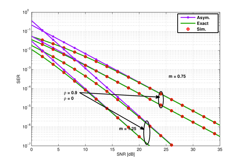
Figure 2: Example SER performance over Nakagami${-}m$ fading channels with $m_{S,D}=m_{S,R}=m_{R,D}=m=\{0.75,1.25\},\,\Omega_{S,D}=\Omega_{S,R}=\Omega_{R,D}=0$dB for $4{-}$QAM/QPSK constellations and different values of spatial correlation.

V System Power Consumption Model and Analysis

In this section, motivated by the general interests towards green communications and increasing incentives to save energy, we quantify the total energy consumption required to transmit information from the source to the destination. We assume that the transceiver circuitry operates on multi-mode basis i.e. $i)$ when there is a signal to transmit, the circuits are in active mode; $ii)$ when there is no signal to transmit, the circuits operate on a sleep mode; $iii)$ the circuits are in transient mode during the switching process from sleep mode to active mode. The elementary block diagrams of the assumed transmitter and receiver are illustrated in Fig. 2 and Fig. 3, respectively. This model is based on the energy and layout area efficient direct-conversion architecture which is commonly used in wireless transceivers. It is also assumed that all nodes are equipped with similar transmitter and receiver circuit blocks and that the power consumption of the active filters at the transmitter and receiver is similar.

Considering a node that transmits $L$ bits and total transmission period $T$, the transient duration from active mode to sleep mode is short enough to be neglected. However, the start-up process from sleep mode to active mode may be slower due to the finite phase-locked loop (PLL) settling time in the frequency synthesizer. By denoting the duration of the sleep, transient and active modes as $T_{sp}$, $T_{tr}$ and $T_{on}$, respectively, the total transmission period is defined as $T=T_{sp}+T_{tr}+T_{on}$, with $T_{tr}$ being equal to the frequency synthesizer settling time. Based on this, the total energy required to transmit and receive $L$ information bits is expressed as

$$E=P_{on}T_{on}+P_{sp}T_{sp}+P_{tr}T_{tr}$$ (30)

where $P_{on},P_{sp}$ and $P_{tr}$ denote the power consumption values during the active, sleep and transient modes, respectively. In realistic circuit designs, the power consumption in the sleep mode can be considered negligible compared to the active mode power [19] and thus, $P_{sp}\simeq 0$. It is also noted that power consumption during the transient mode practically refers to the power consumption of the frequency synthesizers. Based on this, it is assumed that $P_{tr}=2P_{LO}$; therefore, using the power consumption values at both transmitter and receiver sides during the active mode one obtains

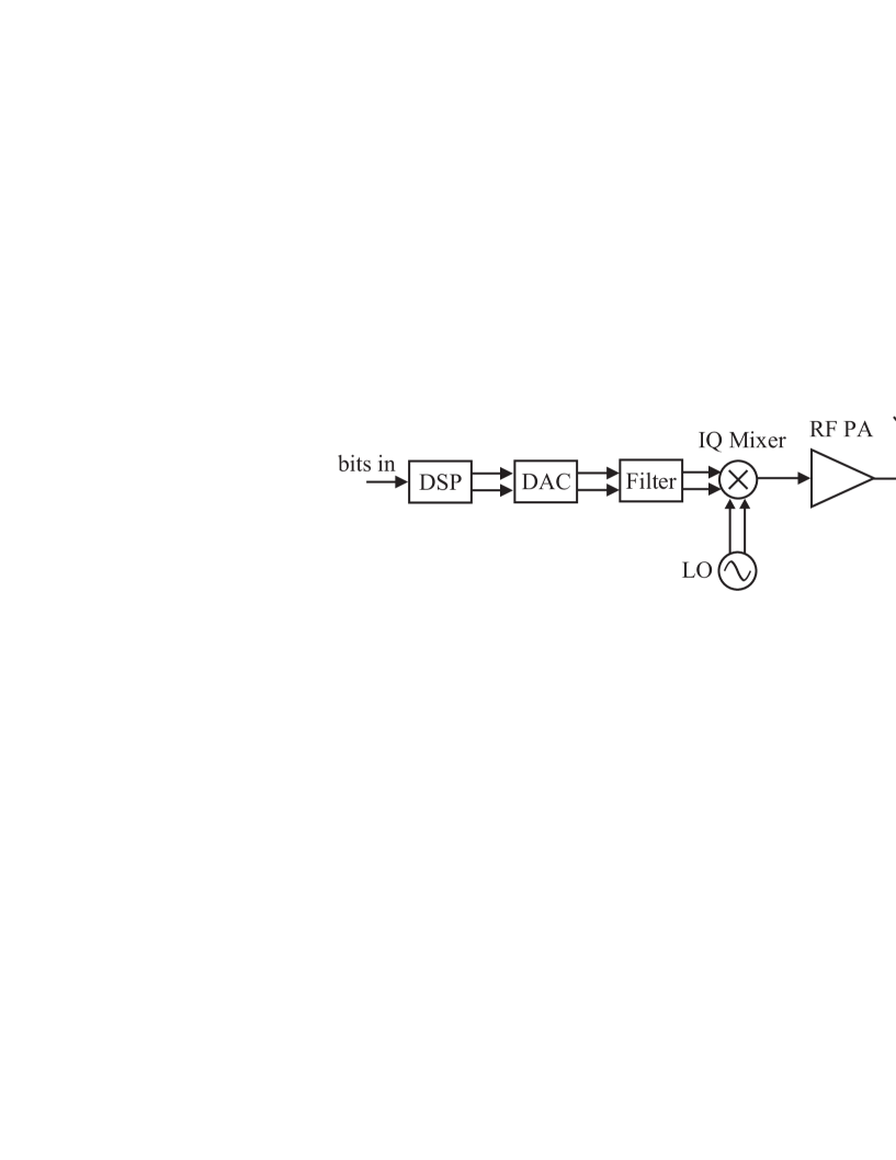
Figure 3: Elementary direct-conversion transmitter.

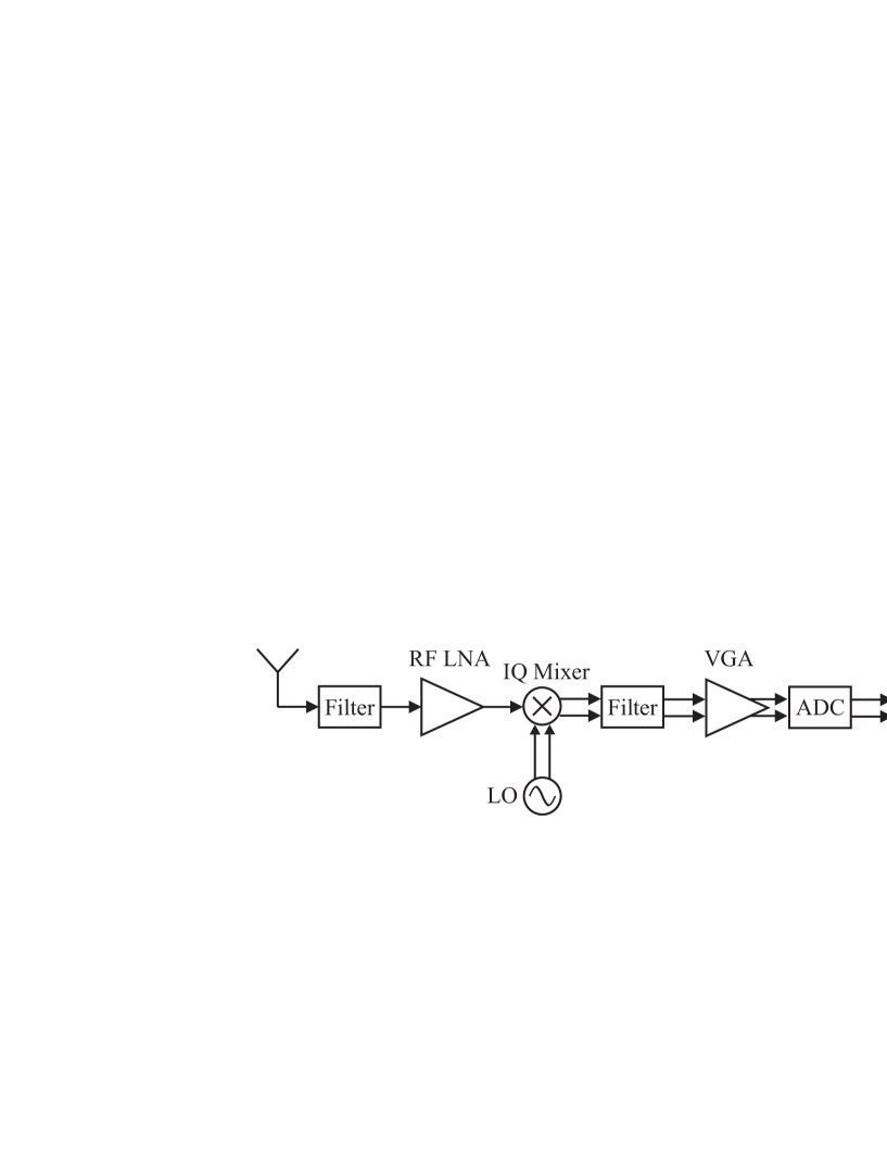
Figure 4: Elementary direct-conversion receiver.

$$P_{on}=P_{ont}+P_{onr}$$ (31)

where $P_{ont}$ is the total transmitter power consumption that accounts for the sum of signal transmission and transmitter circuit powers and $P_{onr}$ is the total receiver power consumption. Hence, it follows that,

$$P_{ont}=P_{t}+P_{amp.}+P_{CT_{x}}$$ (32)

and

$$P_{onr}=P_{CR_{x}}$$ (33)

where $P_{t}$ is the signal transmission power, $P_{amp}$ is the power consumption of the RF power amplifier and $P_{CT_{x}}$ and $P_{CR_{x}}$ denote the total transmitter circuit power and the total receiver circuit powers, namely,

$$P_{CT_{x}}=P_{DSP_{Tx}}+P_{DAC}+P_{Fil}+P_{Mix}+P_{LO}$$ (34)

and

$$P_{CR_{x}}=P_{DSP_{Rx}}+P_{ADC}+P_{VGA}+2P_{Fil}+P_{Mix}+P_{LO}+P_{LNA}$$ (35)

respectively. The $P_{CT_{x}}$ measure consists of the following power consumption entities: digital signal processor (DSP), $P_{DSP_{Tx}}$; digital to analog converter (DAC), $P_{DAC}$; active filter, $P_{Fil}$; IQ Mixer, $P_{Mix}$ and synthesizer, $P_{LO}$. Likewise, the active power consumption at the receiver comprises the power consumption values for digital signal processor (DSP), $P_{DSP_{Rx}}$; analog to digital converter(ADC), $P_{ADC}$; variable gain amplifier (VGA), $P_{VGA}$; active filter, $P_{Fil}$; IQ Mixer, $P_{Mix}$; synthesizer, $P_{LO}$; low noise amplifier (LNA), $P_{LNA}$ [75]. Based on this, the total required circuit power consumption is given by

$$P_{TC}=P_{CT_{x}}+P_{CR_{x}}.$$ (36)

It is also noted that for signal transmission power $P_{t}$, the power consumption of the RF-power amplifier can be modeled by $P_{amp}=\alpha P_{t}$, where $\alpha=\frac{\xi}{\eta}-1$, with $\eta$ and $\xi$ denoting the respective drain efficiency of the amplifier and the peak-to-average power ratio (PAPR), which depends on the modulation order and the associated constellation size. Based on this, for the case of square uncoded $M{-}$QAM modulation, $\xi=3\frac{\sqrt{M}-1}{\sqrt{M}+1}$ and $T_{on}=\frac{LT_{s}}{b}=\frac{L}{bB}$, where $b=\log_{2}M$ is the constellation size, $L$ is the transmission block length in bits  and  $T_{s}$ is the symbol duration which relates to the bandwidth $B$ as $T_{s}\approx\frac{1}{B}$ [23].

VI Energy Optimization and Power Allocation

In this section, we deploy and combine the results of the previous sections and analyze the total energy required to transmit information efficiently from the source to the destination. To this end, we firstly quantify the total energy consumption in the direct communication scenario. Hence, by applying (30), (32) and (33) and recalling that $P_{sp}\approx 0$ and $P_{tr}=2P_{LO}$, the average energy consumption per information bit is given by [76]

$$E^{D}_{T}=\overline{E}^{D}_{T}=\frac{\left((1+\alpha)P_{S}+P_{CT_{x}}+P_{CR_{x}}\right)T_{on}+2P_{LO}T_{tr}}{L}$$ (37)

where $P_{S}$ denotes the source transmit power. In order to determine the average total energy consumption in the corresponding cooperative transmission system deploying the DF protocol, we formulate the total average power consumption, which is a discrete random variable that can be statistically expressed as

$$P_{T}^{C}=\begin{cases}&P_{CT_{x}}+\left(1+\alpha\right)P_{S}+2P_{CR_{x}},\hskip 30.58662pt\text{with}\,\,\,\,{\rm Pr}=1\\ &P_{CT_{x}}+\left(1+\alpha\right)P_{R}+P_{CR_{x}},\hskip 34.14322pt\text{with }\,\,{\rm Pr}=1-\overline{\rm SER}_{S,R}\end{cases}$$ (38)

where $P_{R}$ denotes the relay transmit power. The first term of (38) refers to the absolute total power consumption by the nodes in the first transmission phase, while the second term represents the power consumption in the second phase, subject to correct decoding of the received signal by the relay, which is indicated by the probabilistic term $\left(1-\overline{\rm SER}_{S,R}\right)$. Hence, the average total power consumption in the cooperative transmission mode can be expressed as

$$\bar{P}^{C}_{T}=P_{CT_{x}}+(1+\alpha)P_{S}+2P_{CR_{x}}\;+\;\left(P_{CT_{x}}+(1+\alpha)P_{R}+P_{CR_{x}}\right)\left(1-\overline{\rm SER}_{S,R}\right).$$ (39)

Based on this, the corresponding average energy consumption per information bit is given by

$$\bar{E}^{C}_{T}=\frac{\overline{P}^{\,C}_{T}T_{on}+2P_{LO}T_{tr}}{L}.$$ (40)

The achieved energy efficiency enhancement by the cooperative transmission is determined with the aid of the cooperation gain (CG), which is the ratio of the energy efficiency of cooperative transmission over the energy efficiency of the direct transmission, per successfully delivered bit, namely,

$$CG=\frac{\overline{E}^{D}_{T}\left(1-\overline{\rm BER}^{C}_{D}\right)}{\overline{E}^{C}_{T}\left(1-\overline{\rm BER}^{D}_{D}\right)}.$$ (41)

Evidently, when the resulting ratio is smaller than one, it indicates that direct transmission is more energy efficient and thus, the extra energy consumption induced by cooperation outweighs its gain in decreasing the BER of the system.

In what follows, the above expressions are employed in formulating and solving the energy optimization problems aiming to guarantee certain QoS requirements, namely, target destination BER. In the same context, we additionally provide the optimal power allocation formulation for the cooperative transmission scenario under the maximum total transmit power constraint.

VI-A Direct Transmission

We first consider the energy optimization problem for minimizing the average total energy consumption in the direct communication scenario with the maximum transmission power and target bit error rate, $p^{*}$, as constraints. We assume that the power consumption of the circuit components are fixed and independent of the optimization. Thus, the only variable in the optimization is the transmit power of the source. To this effect and with the aid of (37), the optimization problem for the direct transmission mode can be formulated as follows:

$$\begin{split}\min_{P_{S}}\overline{E}^{D}_{T}\hskip 113.81102pt\\ \quad\text{subject to:}\>\>\>P_{S}\leq P_{maxt},\quad P_{S}\geq 0\hskip 56.9055pt\\ \overline{\rm BER}^{D}_{D}=p^{*}.\hskip 99.58464pt\end{split}$$ (42)

Deriving the minimum average total energy required in the direct communication scenario, requires prior computation of the corresponding symbol error probability. This is realized with the aid of (8) which is expressed in closed-form in terms of ${}_{2}F_{1}\left(m,\frac{1}{2};m+1;\frac{1}{1+a_{1}}\right)$ and $F_{1}\left(\frac{1}{2};\frac{1}{2}-m,m,\frac{3}{2};\frac{1}{2},\frac{1}{2+2a_{1}}\right)$ functions. It is recalled that these functions are widely employed in natural sciences and engineering and their computational implementation is rather straightforward as they are built-in functions in popular software packages such as MATLAB, MAPLE and MATHEMATICA. It is also noted that the representation of these functions in the present analysis allows the following useful approximative expressions: ${}_{2}F_{1}\left(m,\frac{1}{2};m+1;\frac{1}{1+a_{1}}\right)\simeq 1$ and $F_{1}\left(\frac{1}{2};\frac{1}{2}-m,m,\frac{3}{2};\frac{1}{2},\frac{1}{2+2a_{1}}\right)\simeq F_{1}\left(\frac{1}{2};\frac{1}{2}-m,m,\frac{3}{2};\frac{1}{2},0\right)$. The accuracy of these approximations is validated through extensive numerical and simulation results which indicate their tightness for random values of $m$ and moderate and large values of $a_{1}$. To this effect, the following accurate closed-form BER approximation for $M{-}$QAM modulated signals is deduced

$$\overline{\rm BER}^{D}_{D}\simeq\frac{2\;(\sqrt{M}-1)\Gamma(m+\frac{1}{2})}{\sqrt{\pi}Mm!(1+a_{1})^{m}\log_{2}M}+\frac{4\,F_{1}(\frac{1}{2};\frac{1}{2}-m,m,\frac{3}{2};\frac{1}{2},0)}{\sqrt{2}\pi(1+a_{1})^{m}\log_{2}M}\left(1-\frac{1}{\sqrt{M}}\right)^{2}.$$ (43)

Importantly, the Appell function in (43) can be expressed in terms of the Gauss hypergeometric function,

$$F_{1}\left(\frac{1}{2};\frac{1}{2}-m,m,\frac{3}{2};\frac{1}{2},0\right)=\,_{2}F_{1}\left(\frac{1}{2},\frac{1}{2}-m;\frac{3}{2},\frac{1}{2}\right).$$ (44)

As a result, equation (43) becomes

$$\overline{\rm BER}^{D}_{D}\simeq\frac{2\;(\sqrt{M}-1)\Gamma(m+\frac{1}{2})}{\sqrt{\pi}Mm!(1+a_{1})^{m}\log_{2}M}+\frac{4\,\,_{2}F_{1}\left(\frac{1}{2},\frac{1}{2}-m;\frac{3}{2},\frac{1}{2}\right)}{\sqrt{2}\pi(1+a_{1})^{m}\log_{2}M}\left(1-\frac{1}{\sqrt{M}}\right)^{2}.$$ (45)

It is evident that (45) is a function of the modulation order, the severity of multipath fading and $a_{1}$. Therefore, by substituting the targeted QoS $p^{*}$ in (45), recalling that $a_{1}=(P_{S}\>\>\Omega_{S,D}\>g_{QAM}){/}(N_{0}P_{L_{S,D}})\>$ and carrying out some algebraic manipulations, one obtains

$$P_{S}\simeq\frac{mN_{0}P_{L_{S,D}}}{\Omega_{S,D}g_{QAM}}\left[\left(\frac{C}{p^{*}}\right)^{1/m}-1\right]$$ (46)

where

$$C=\frac{4(\sqrt{M}-1)}{M\log_{2}M}\left[\frac{(\sqrt{M}-1)\,_{2}F_{1}\left(\frac{1}{2},\frac{1}{2}-m;\frac{3}{2};\frac{1}{2}\right)}{\sqrt{2}\>\pi}+\frac{\;\Gamma(m+\frac{1}{2})}{2\sqrt{\pi}m\Gamma(m)}\right].$$ (47)

To this effect and with the aid of (37) and (46), it follows that the minimum total energy per information bit required for direct transmission for meeting the required QoS can be expressed in closed-form as

$$\overline{E}^{D*}_{T}=\frac{\left(P_{CT_{x}}+P_{CR_{x}}\right)T_{on}}{L}+\frac{(1+\alpha)N_{0}m_{S,D}T_{on}P_{L_{S,D}}}{L\,\Omega_{S,D}g_{QAM}}\left[\left(\frac{C}{p^{*}}\right)^{1/m}-1\right]+\frac{2P_{LO}T_{tr}}{L}.$$ (48)

Based on the total energy consumption in (48) and given the constellation size $b=\frac{L}{BT_{on}}$, it is shown that the proposed energy expression comprises the transmission energy $E_{t}$ and circuit energy $E_{C}$, namely,

$$E_{t}=P_{S}T_{on}=\frac{N_{0}mPL_{S,D}}{\Omega_{S,D}g_{QAM}}\left[\left(\frac{C}{p^{*}}\right)^{1/m}-1\right]\frac{T_{on}}{L}$$ (49)

where $C$ can be expressed as a function of the transmission time $T_{on}$ as follows

$$C=\frac{BT_{on}\,\left(2^{\frac{L}{2BT_{on}}}-1\right)^{2}}{L\pi 2^{\frac{L}{BT_{on}}-\frac{3}{2}}}\,\,_{2}F_{1}\left(\frac{1}{2},\frac{1}{2}-m;\frac{3}{2};\frac{1}{2}\right)+\frac{2BT_{on}}{2^{\frac{L}{BT_{on}}}mL\sqrt{\pi}}\,\left(\frac{1}{2}\right)_{m}\left(2^{\frac{L}{2BT_{on}}}-1\right).$$ (50)

Hence, by inserting (50) in (49), the following analytic expression for the transmission energy per information bit is deduced

$$E_{t}=\frac{N_{0}mPL_{S,D}T_{on}}{L\,\Omega_{S,D}g_{QAM}}\left\{\left[\frac{BT_{on}\,\left(2^{\frac{L}{2BT_{on}}}-1\right)^{2}}{p^{*}L\pi 2^{\frac{L}{BT_{on}}-\frac{3}{2}}}\,\,_{2}F_{1}\left(\frac{1}{2},\frac{1}{2}-m;\frac{3}{2};\frac{1}{2}\right)+\frac{BT_{on}\left(2^{\frac{L}{2BT_{on}}}-1\right)}{p^{*}mL\sqrt{\pi}\;2^{\frac{L}{BT_{on}}-1}}\,\left(\frac{1}{2}\right)_{m}\right]^{1/m}-1\right\}.$$ (51)

Likewise, the circuit energy, $E_{C}$, can be expressed as

$$E_{C}=\left(P_{CT_{x}}+P_{CR_{x}}\right)T_{on}.$$ (52)

Notably, equations (50) and (51) indicate that for a fixed bandwidth $B$ and packet length $L$, the transmission energy is a decreasing function with respect to the product $T_{on}B$ whereas the circuit energy increases monotonically with respect to $T_{on}$. In addition, it is shown that the transmission energy is dependent upon the transmission distance $d_{S,D}$ and the severity of fading $m$, while the corresponding circuit energy remains fixed regardless of the value of $d_{S,D}$ and $m$.

VI-B Cooperative Transmission

This subsection presents the energy optimization and power allocation problem when the involved relay forwards successfully decoded signals, generally at different power than the power of the source. Evidently, the respective optimization model is a two dimensional problem and thus, we formulate the energy minimization problem with two optimization variables, namely, the source transmit power, $P_{S}$, and the relay transmit power, ${P}_{R}$. In this context, the aim is to minimize the total energy consumption of the overall network instead of minimizing the energy consumption at individual nodes. Based on this and with the aid of (40), the optimization problem can be formulated as follows:

$$\begin{split}\hskip 113.81102pt\min_{P_{S},{P}_{R}}\overline{E}^{C}_{T}(P_{S},{P}_{R})\hskip 113.81102pt\\ \quad\text{subject to:}\quad(P_{S}+{P}_{R})\leq P_{maxt},\quad P_{S}\geq 0,\quad{P}_{R}\geq 0\hskip 56.9055pt\\ \vspace{0.5cm}\overline{\rm BER}^{C}_{D}(P_{S},{P}_{R})=p^{*}.\hskip 99.58464pt\end{split}$$ (53)

The above optimization task is a non-linear programming problem since the objective function and the constraint BER are both non-linear functions of $P_{s}$ and ${P}_{R}$. It is also recalled that Karush Kuhn Tucker (KKT) conditions that handle both equality and inequality constraints are in general the first order sufficient and necessary conditions for optimum solutions in non-linear optimization problems (NLP) provided that certain regularity conditions are satisfied. To this end, using the Lagrange multipliers $\lambda_{1}$ and $\lambda_{2}$, $\lambda_{3}$ and $\lambda_{4}$, for the equality and inequality constraints we set the corresponding Lagrangian equation that depends on the optimization variables and multipliers while meeting the KKT conditions in [77] for the non-linear convex optimization problem, namely

$$L=\overline{E}^{C}_{T}+\lambda_{1}\left(\overline{\rm BER}^{C}_{D}-p^{*}\right)-\lambda_{2}P_{S}-\lambda_{3}{P}_{R}+\lambda_{4}\left(\left(P_{S}+{P}_{R}\right)-P_{maxt}\right).$$ (54)

The proof for the convexity of the optimization problem is provided in Appendix E.

Based on (54), the KKT conditions for the problem can be expressed as follows:

$$\nabla\overline{E}^{C}_{T}+\lambda_{1}\nabla\overline{\rm BER}^{C}_{D}-\lambda_{2}\nabla P_{S}-\lambda_{3}\nabla{P}_{R}+\lambda_{4}\nabla\left(P_{S}+{P}_{R}\right)=0$$ (55)

whereas the associated complementary conditions are given by

$$\begin{split}\overline{\rm BER}^{C}_{D}=p^{*},\,P_{S}+{P}_{R}\leq P_{maxt}\hskip 85.35826pt\\ \lambda_{1}\left(\overline{\rm BER}^{C}_{D}-p^{*}\right)=0,\,\,\lambda_{2}P_{S}=0,\,\,\lambda_{3}{P}_{R}=0\,\>\,\text{and}\,\>\lambda_{4}\left(P_{S}+{P}_{R}-P_{maxt}\right)=0\\ \lambda_{1},\lambda_{2},\lambda_{3},\lambda_{4}\geq 0.\hskip 142.26378pt\end{split}$$ (56)

In the above set of complementary KKT conditions both $\lambda_{2}$ and $\lambda_{3}$ represent inactive constraints and therefore, they can be assumed zero. To this effect, by applying (55) and setting the derivatives w.r.t $P_{S}$ and ${P}_{R}$ to zero, the following useful set of equations is deduced

$$\frac{\partial\overline{E}^{C}_{T}}{\partial P_{S}}\>+\,\,\lambda_{1}\frac{\partial\overline{\rm BER}^{C}_{D}}{\partial P_{S}}\,\,+\lambda_{4}=0$$ (57)

and

$$\frac{\partial\overline{E}^{C}_{T}}{\partial{P}_{R}}\>+\,\,\lambda_{1}\frac{\partial\overline{\rm BER}^{C}_{D}}{\partial{P}_{R}}\,\,+\lambda_{4}=0.$$ (58)

Solving for $\lambda_{4}$ from (57) and substituting in (58) yields the following relationship which depends only on one of the Lagrangian multipliers

$$\frac{\partial\overline{E}^{C}_{T}}{\partial P_{S}}\>-\frac{\partial\overline{E}^{C}_{T}}{\partial{P}_{R}}\>+\,\,\lambda_{1}\left(\frac{\partial\overline{\rm BER}^{C}_{D}}{\partial P_{S}}-\frac{\partial\overline{\rm BER}^{C}_{D}}{\partial{P}_{R}}\right)=0$$

and

$$\lambda_{1}=\frac{\frac{\partial\overline{E}^{C}_{T}}{\partial P_{S}}\>-\frac{\partial\overline{E}^{C}_{T}}{\partial{P}_{R}}}{\left(\frac{\partial\overline{\rm BER}^{C}_{D}}{\partial{P}_{R}}-\frac{\partial\overline{\rm BER}^{C}_{D}}{\partial P_{S}}\right)}.$$ (59)

Based on this and using the fact that $\lambda_{1}\geq 0$, one obtains the following necessary condition for minimizing the total average energy consumption of the cooperative transmission mode at the optimal power values

$$\frac{\partial\overline{E}^{C}_{T}(P_{S}^{\,*},P_{R}^{\,*})}{\partial P_{S}}\,\geq\,\frac{\partial\overline{E}^{C}_{T}(P_{S}^{\,*},P_{R}^{\,*})}{\partial{P}_{R}}.$$ (60)

For a feasible set of optimal powers, the $\overline{\rm BER}^{C}_{D}=p^{*}$ and $P_{S}+{P}_{R}\leq P_{maxt}$ constraints must be satisfied.

Analytic solution for the optimal powers in (60) is intractable to derive in closed form. However, this can be alternatively realized with the aid of numerical optimization techniques, which can determine the optimal powers at the source and relay nodes that minimize the average total energy consumption. To this end, we employ the MATLAB optimization tool box and its function fimincon in the respective numerical calculations for allocating the available power optimally under the given constraints. Thus, the derived expressions and offered results provide tools to understand, quantify and analyze how much energy can in general be saved, per successfully communicated bit in the system, if transmit power allocation and optimization beyond classical equal power allocation is pursued in the cooperative system, on one side, and how much energy can be saved against the classical non-cooperative (direct transmission) system, on the other side. Furthermore, the considered values in the present paper are indicative and are selected in the context of demonstrating the validity of the proposed method. Therefore, the derived optimization flow can be readily extended to arbitrary design constraints for the total network power consumption and target destination error rate in the presence of Nakagami$-{m}$ multipath fading conditions.

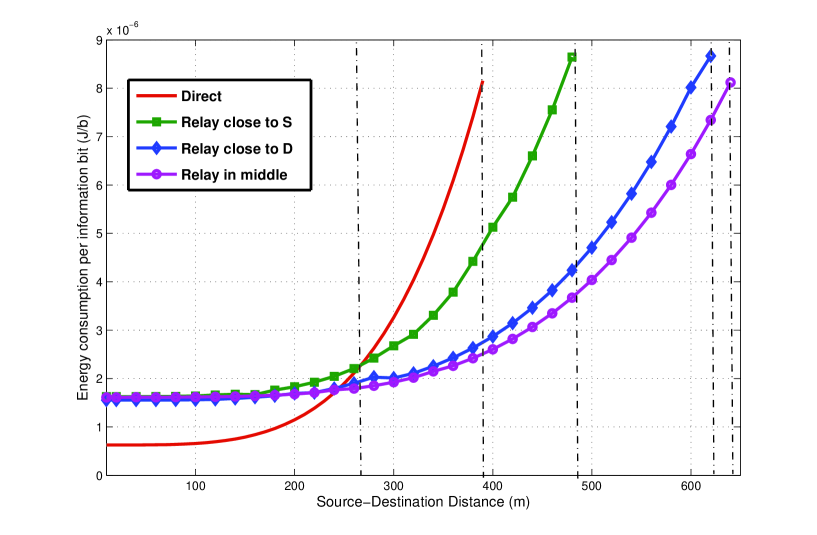
Figure 5: Energy consumption per information bit versus source-destination distance for different relay locations over uncorrelated Nakagami${-}1.25$ at target BER of $10^{-2}$ for $4{-}$QAM / QPSK constellation.

VII Numerical Results and Analysis

This section demonstrates and evaluates the average total energy consumption of the considered regenerative system assuming that the S-D and S-R links are statistically independent whereas the S-D and R-D paths are spatially correlated. As a realistic example, we assume $M{-}$QAM modulation scheme over the S-D, S-R and R-D links, in case of cooperative transmission mode, and over the S-D link in the case of only direct communication. For the sake of simplicity, it is also assumed that all wireless channels are subject to Nakagami${-}m$ multipath fading conditions with $\Omega_{S,D}=\Omega_{S,R}=\Omega_{R,D}=0$dB. The involved path-loss effects are modeled by an example model of $P_{L_{i,j}}\,[{\rm dB}]=148+40\log_{10}(d_{i,j}[{\rm km}])$, which is also used in device-to-device based communications [70], and thus applies to mobile relaying as well. Furthermore, in order to simplify the geometry-related calculations, we assume that all nodes are located along a straight line, which satisfies the distance relationship $d_{S,D}=d_{S,R}+d_{R,D}$. However, it is recalled here that the path-loss and distance assumptions are only indicative in the context of the considered examples, while the provided analysis and optimization frameworks are valid more generally. In this context, we further assume the following system parameters: $N_{0}=-174\text{dBm/Hz}$; $\eta=0.35$; $T_{tr}=5{\rm\mu}s$; $L=2\text{kbits}$, and $P_{LO}=50\text{mW}$ [23, 19]. We also use the constant circuit powers as $P_{CT_{x}}=100\text{mW}$, $P_{CR_{x}}=150\text{mW}$ and the maximum transmission power $P_{maxt}=1000\text{mW}$. The bandwidth of the system is assumed to be $B=200\text{kHz}$ and the noise figure $N_{f}=6\text{dB}$. Due to the linearity requirement of the $M{-}$QAM signals, the value of the drain efficiency is assumed $\eta=0.35$, which is a practical value for class-A and AB RF power amplifiers (PA). The considered system parameters are depicted in Table I and are used unless otherwise stated.

TABLE I: Assumed System Parameters

$N_{0}=\text{-174dBm/Hz}$	$N_{f}=\text{6dB}$
$B=\text{200kHz}$	$L=\text{2kbits}$
$P_{CT_{x}}=\text{100mW}$	$P_{CR_{x}}=\text{150mW}$
$P_{LO}=\text{50mW}$	$P_{maxt}=\text{1000mW}$
$\eta=0.35$	$T_{tr}=5\mu s.$

We commence by analyzing the minimum energy per information bit required for the direct and cooperative transmissions when the relay node is taken into account and placed in different locations. The location of the relay node is represented with parameter $f=d_{S,R}/d_{S,D}$. Fig. 5 illustrates the total energy consumption per information bit as a function of the transmission distance from source to destination for $4-$QAM/QPSK with fading parameter of $m=1.25$, destination target BER of $10^{-2}$ and zero spatial correlation under the maximum transmit power constraint. The transmit power allocation is carried out by the derived OPA scheme resulting to the indicative values in Table II. It is observed that distance thresholds separate the regions where DT performs better than CT and vice-versa. Furthermore, it is shown that when the relay is located in the middle, i.e. the source-relay distance equals the relay-destination distance ($f=0.5$), renders the best energy efficiency among all relay locations. This indicates that the configuration is almost symmetric in the source-relay and relay-destination distances, which assists the system to operate robustly in transmission over severe fading conditions. However, it is shown that at relatively small distances (here $0\leq d_{S,D}\leq 170m$), the exact location of the relay does not affect substantially the performance of the cooperative system as it appears to remain almost the same in all considered scenarios. This renders the relay positioning and planning rather simple when the relay falls within this range, while it additionally provides insight e.g. for relay selection algorithms in the case of randomly distributed relays in emerging relay-based wireless networks.

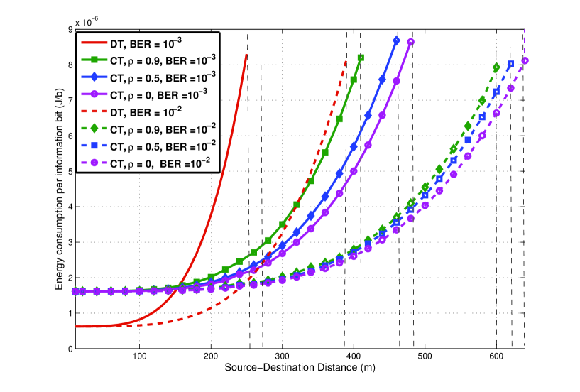
Figure 6: Energy consumption per information bit versus source-destination distance when the relay is located in the middle over spatially correlated Nakagami${-}1.25$ for $4{-}$QAM/QPSK constellations with different target BERs.

TABLE II: Optimal Transmit Power Values for Source and Relay for Different Relay Locations over Uncorrelated Nakagami${-}1.25$ Links at target BER of ${10^{-2}}$ for $4{-}$QAM / QPSK Modulation.

	Relay close to $S\;(f=0.1)$		Relay in middle  $(f=0.5)$		Relay close to $D\;(f=0.9)$
D(m)	$P_{S}(\text{W})$	$P_{R}(\text{W})$	$P_{S}(\text{W})$	$P_{R}(\text{W})$	$P_{S}(\text{W})$	$P_{R}(\text{W})$
100	0.00033	0.0006	0.000312	0.000197	0.000651	0.00049
200	0.016	0.0127	0.0057	0.0033	0.0104	0.0101
300	0.0877	0.0595	0.0289	0.0223	0.0527	0.0525
400	0.3366	0.1537	0.0706	0.0703	0.1666	0.0198
480	0.6225	0.3601	0.1466	0.1455	0.3455	0.0342
620	-	-	0.4107	0.402	0.9627	0.0373
650	-	-	0.4970	0.483	-	-

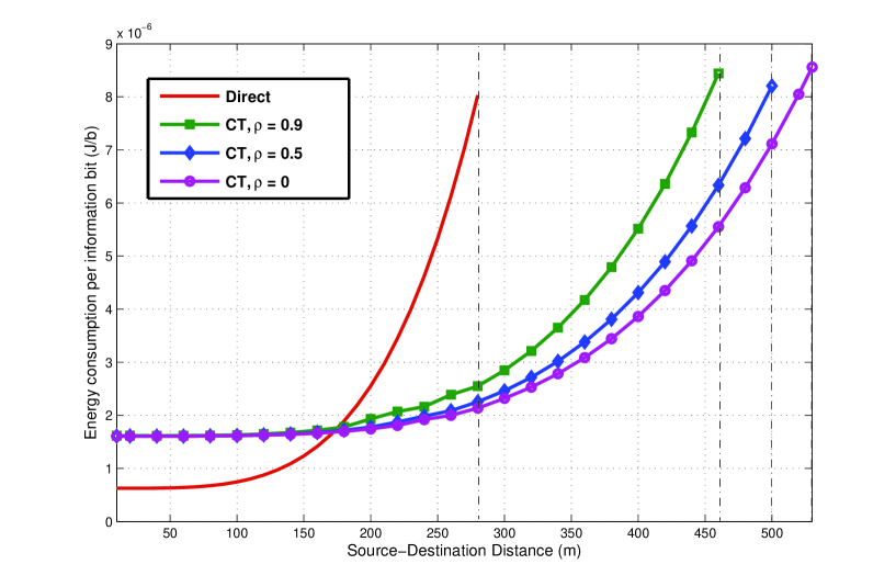
Figure 7: Energy consumption per information bit versus source-destination distance when the relay is located in the middle over spatially correlated Nakagami${-}0.75$ fading channels at target BER of $10^{-2}$ for $4{-}$QAM/QPSK constellation and different spatial correlation values.

The corresponding energy efficiency is also analyzed for target BERs of $10^{-2}$ and $10^{-3}$. Fig. 6 illustrates the average total energy consumption per information bit for $4-$QAM${/}$QPSK in both direct and cooperative transmissions in Nakagami${-}1.25$ fading conditions under the maximum transmit power constraint and the following spatial correlation scenarios: $\rho=\{0,0.5,0.9\}$. Also, the relay node is located in the middle and the transmit power is allocated optimally to the source and relay nodes in all cases. It is observed that for the fixed target BERs of $10^{-2}$ and $10^{-3}$, the direct scheme outperforms the cooperative transmission only at average source-destination distances below 240m and 150m, respectively. On the contrary, for average distances greater than 240m and 150m, CT becomes more energy efficient as the transmit power constitutes a significant share of the average total energy consumption even under the worst spatial correlation scenario. Furthermore, it is shown that for the given target BERs the DT schemes attain maximum transmission distances of 390m and 250m, respectively, under the given maximum transmission power constraint while in both cases the cooperative transmission schemes extend to substantially longer distances. However, these advantages vary according to the level of the involved spatial correlation where the improvement in energy efficiency is inversely proportional to $\rho$, in both scenarios. The reason is that for every step of transmission distance, greater proportion of power is assigned to the source and relay nodes in order to overcome performance losses incurred by the spatial correlation, within the given resource constraints. Concrete examples are shown in Table III and Table IV for some indicative transmission distances and the two target BERs; there, the energy savings using CT scheme, defined as $1-\overline{E}^{C}/\overline{E}^{D}$ for $\rho=0.9$, $\rho=0.5$ and $\rho=0$ for the target BER of $10^{-2}$ at $d_{S,D}=390$m are $65\%$, $67\%$ and $69.3\%$, respectively, whereas for a target BER of $10^{-3}$ at $d_{S,D}=250$m the energy reduction is $69\%,72\%\;\text{and}\;73.8\%$, respectively. Interestingly, beyond a critical distance of 320m, even the highly spatially correlated CT mode at target BER of $10^{-3}$ exhibits better energy-efficiency than the DT scheme with target BER of $10^{-2}$.

TABLE III: Optimal Transmit Power Values for Source and Relay for relay located in the middle over correlated Nakagami${-}1.25$ Links with target BER of ${10^{-2}}$ Using $4{-}$QAM ${/}$ QPSK Modulation.

Corr.	$\rho=0$		$\rho=0.5$		$\rho=0.9$
D(m)	$P_{S}(\text{W})$	$P_{R}(\text{W})$	$P_{S}(\text{W})$	$P_{R}(\text{W})$	$P_{S}(\text{W})$	$P_{R}(\text{W})$
100	0.000372	0.000197	0.000424	0.000233	0.000514	0.000296
200	0.0057	0.0033	0.0064	0.0039	0.0077	0.0049
300	0.0225	0.0223	0.0249	0.0249	0.0290	0.0290
400	0.0706	0.0703	0.0788	0.0785	0.0918	0.0915
500	0.1728	0.1712	0.1929	0.1912	0.2249	0.2228
600	0.3598	0.3530	0.4021	0.3944	0.4692	0.4602
630	0.4381	0.4281	0.4897	0.4785	-	-
650	0.4970	0.4843	-	-	-	-

In the same context, Fig. 7 illustrates the average total energy per information bit for both direct and cooperative transmissions for $m=0.75$, which corresponds to severe fading conditions. The target BER is set to $10^{-2}$ under the given transmit power constraint while $\rho=\{0,0.5,0.9\}$. The transmit power is again allocated optimally to the source and relay with the latter positioned in the center of the network as shown in Table V. It is shown that DT outperforms CT only when $d_{S,D}\leq 170m$. However, as the distance increases beyond this point, the corresponding overall benefits by CT are significant even under the worst spatial correlation scenario. Indicatively, at a transmission distance of 280m, which is the maximum distance that DT can operate with the available maximum transmission power, the energy gains by CT are $68\%$, $72\%$ and $74\%$, respectively. In addition, it is shown that the advantage of the cooperation is more significant in severe fading conditions.

TABLE IV: Optimal Transmit Power Values for Source when the Relay is Located in the Middle over Correlated Nakagami${-}1.25$ Links with Target BER of ${10^{-3}}$ Using $4{-}$QAM ${/}$ QPSK Constellations.

Corr.	$\rho=0$		$\rho=0.5$		$\rho=0.9$
D(m)	$P_{S}(\text{W})$	$P_{R}(\text{W})$	$P_{S}(\text{W})$	$P_{R}(\text{W})$	$P_{S}(\text{W})$	$P_{R}(\text{W})$
100	0.00012	0.0007	0.00014	0.0009	0.00022	0.00014
200	0.0179	0.0116	0.0218	0.0147	0.0331	0.0233
300	0.0762	0.0762	0.0914	0.0914	0.1332	0.1332
410	0.2662	0.2651	0.3196	0.3183	0.4660	0.4641
440	0.3533	0.3513	0.4242	0.4218	-	-
480	0.5009	0.4969	-	-	-	-

TABLE V: Optimal Transmit Power Values for Source and Relay when the Relay is Located in the Middle over Spatially Correlated Nakagami${-}0.75$ Links with target BER of ${10^{-2}}$ Using $4{-}$QAM ${/}$ QPSK Modulations.

Corr.	$\rho=0$		$\rho=0.5$		$\rho=0.9$
D(m)	$P_{S}(\text{W})$	$P_{R}(\text{W})$	$P_{S}(\text{W})$	$P_{R}(\text{W})$	$P_{S}(\text{W})$	$P_{R}(\text{W})$
100	0.000754	0.0004635	0.0009112	0.0005811	0.00013	0.0009
200	0.0119	0.0076	0.0143	0.0093	0.0386	0.0097
300	0.0509	0.0509	0.0608	0.0608	0.0873	0.0873
400	0.1612	0.1606	0.1926	0.1918	0.2765	0.2753
460	0.2823	0.2802	0.3373	0.3348	0.4845	0.4808
500	0.3945	0.3905	0.4714	0.4666	-	-
530	0.4985	0.4921	-	-	-	-

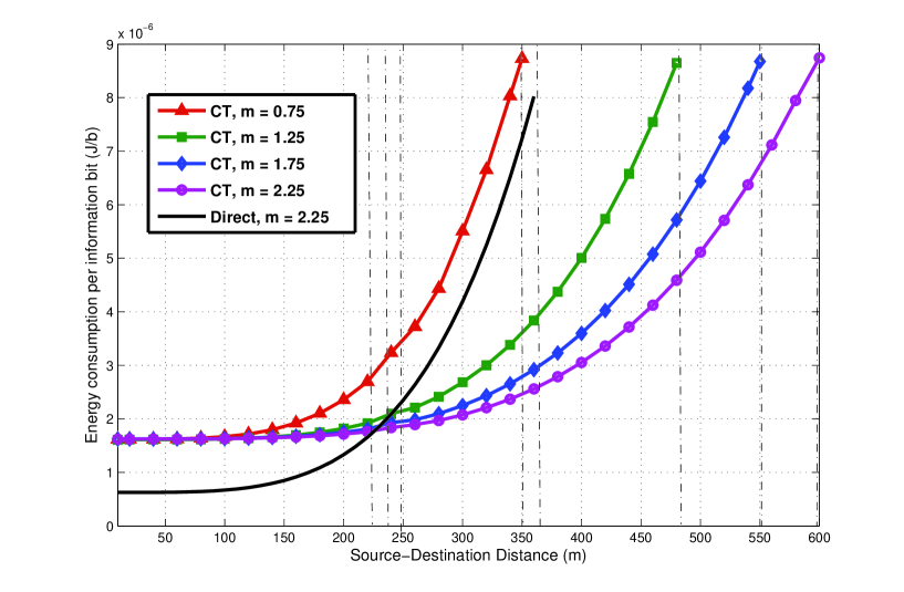
Figure 8: Energy consumption per information bit versus source-destination distance when the relay is located in the middle over uncorrelated Nakagami${-}m$ fading conditions at target BER of $10^{-3}$ for $4{-}$QAM ${/}$ QPSK constellation.

Fig. 8 illustrates the average total energy consumption per information bit required for CT and DT as a function of S-D distance for fading parameters, $m=\{0.75,1.25,1.75,2.25\}$ for CT and $m=2.25$ for DT. The target BER is set to $10^{-3}$, the transmit power is allocated optimally, the relay is located in the middle and a zero spatial correlation is assumed. It is observed that the critical distances below which DT outperforms the CT in terms of energy efficiency are 250m, 230m and 220m for $m=1.25,m=1.75,\text{and}\;m=2.25$ , respectively. Moreover, the analysis indicates that DT with non-severe multipath fading condition (Nakagami${-2.25}$) can operate only up to 360m before utilizing the maximum transmit power, while the CT extends significantly even for moderate fading conditions, except for the worst case scenario ($m=0.75$). It is also shown that the gain from the cooperation is not uniform as the Nakagami parameter increases from $m=0.75$ to $m=1.25$, from $m=1.25$ to $m=1.75$ and then from $m=1.75$ to $m=2.25$.

Finally, Fig. 9 depicts the cooperation gain, defined in (41), when the relay is located in the middle of the source and destination. The power allocation is again carried out by using the derived OPA scheme for target BER of $10^{-2}$ under the maximum transmission power constraint with $\rho=\{0,0.5,0.9\}$ for $m=1.25$. The transmission distance is limited to 390m since beyond this limit it is only the CT mode that can transmit until its maximum transmission distance, depending on the spatial correlation between S-D and R-D paths. When the cooperation gain is below unity, the DT is actually more energy efficient than CT. As already mentioned, the reason behind this is that when $CG\leq 1$, which corresponds to relatively small transmission distances, the actual transmit power constitutes only a small fraction of the total average power consumption. However, when $CG>1$, the system benefits significantly from cooperation and in general CG increases proportionally as the transmission distance increases for all scenarios of spatial correlation between the S-D and R-D paths. Interestingly, the existence of such efficiency threshold distance also implies that a hybrid system, where cooperation is only sought and deployed beyond certain minimum distance, can provide the most comprehensive solution to the energy-efficiency optimization. The analysis and modeling results and tools provided in this article form directly the basis for further development of such schemes in different communication scenarios, which forms an important topic of future work.

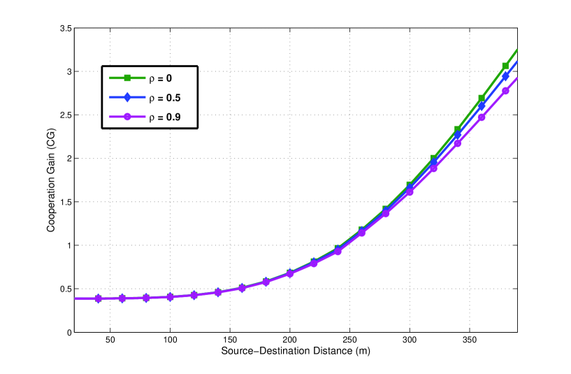
Figure 9: Cooperation gain versus source-destination distance when the relay is located in the middle over spatially correlated Nakagami${-}1.25$ fading environment at target BER of $10^{-2}$ for $4{-}$QAM ${/}$ QPSK constellations. After source-destination distance of 390m, direct transmission runs out of power and cannot anymore reach the target BER.

VIII Conclusions

This work was devoted to the end-to-end SER analysis as well as the energy efficiency analysis and optimization of both direct and regenerative cooperative transmissions over Nakagami${-m}$ fading conditions in the presence of spatial correlation. Novel closed-form expressions were firstly derived for the symbol-error rate of both $M-$QAM and $M-$PSK constellations which were subsequently employed in formulating the constrained energy analysis and optimization problems under destination bit-error-rate target and maximum transmit power constraints considering both transmit energy as well as the energy consumed by the transceiver circuits. The corresponding results indicate that depending on the severity of multipath fading, spatial correlation between the source-destination and relay-destination paths and the location of the relay node, the direct transmission can be more energy efficient than cooperative transmission but only for rather short transmission distances and up to a certain threshold value. Beyond this value, the system, as expected, benefits substantially from relaying and the corresponding cooperation gain increases proportionally to the transmission distance. It is expected that the offered results can be useful in the design, dimensioning and deployment of low-cost and energy efficient cooperative communication systems in the future, especially towards the green communications era where the requirements and incentives towards energy consumption optimization are considered critical.

Appendix

VIII-A Proof of Theorem $1$

The average SER for the direct transmission can be expressed as,

$$\overline{\rm SER}^{D}_{D}=F_{QAM}\left[\left(1+\frac{(P_{S}/\>P_{L_{S,D}})\>\Omega_{S,D}\>g_{QAM}}{N_{0}\>m_{S,D}\,{\sin}^{2}(\theta)}\right)^{-m_{S,D}}\right].$$ (61)

Evidently, a closed-form expression for (61) is subject to analytic evaluation of the following integrals

$$\mathcal{I}\left(a,m;0,\frac{\pi}{2}\right)=\int_{0}^{\pi{/}2}\frac{1}{\left(1+\frac{a}{{\sin}^{2}(\theta)}\right)^{m}}d\theta$$ (62)

and

$$\mathcal{I}\left(a,m;0,\frac{\pi}{4}\right)=\int_{0}^{\pi{/}4}\frac{1}{\left(1+\frac{a}{{\sin}^{2}(\theta)}\right)^{m}}{\rm d}\theta.$$ (63)

By re-writing the indefinite form of the above class of integrals as

$$\mathcal{I}(a,m)=\int\frac{\sin^{2m}(\theta)}{\left(\sin^{2}(\theta)+a\right)^{m}}{\rm d}\theta$$ (64)

and setting $u=\cos^{2}(\theta)$, one obtains

$$\mathcal{I}(a,m)=-\int\frac{(1-u)^{m-\frac{1}{2}}}{2\sqrt{u}(1-u+a)^{m}}{\rm d}u.$$ (65)

The above integral can be expressed in closed-form in terms of the Appell hypergeometric function of the first kind, namely

$$\mathcal{I}(a,m)=-\frac{\cos(\theta)}{(1+a)^{m}}F_{1}\left(\frac{1}{2},\frac{1}{2}-m,m,\frac{3}{2},\cos^{2}(\theta),\frac{\cos^{2}(\theta)}{1+a}\right).$$ (66)

Equation (66) reduces to zero when $\theta=\pi{/}2$. To this effect, it immediately follows that

$$\mathcal{I}\left(a,m,0,\frac{\pi}{2}\right)=\frac{1}{(1+a)^{m}}F_{1}\left(\frac{1}{2},\frac{1}{2}-m,m,\frac{3}{2},1,\frac{1}{1+a}\right)$$ (67)

which with the aid of the properties of $F_{1}(.)$ function can be equivalently expressed as

$$\mathcal{I}\left(a,m,0,\frac{\pi}{2}\right)=\frac{\sqrt{\pi}\Gamma\left(m+\frac{1}{2}\right)}{2(1+a)^{m}\Gamma(m+1)}\,_{2}F_{1}\left(\frac{1}{2},m,m+1,\frac{1}{1+a}\right).$$ (68)

In the same context,

$$\mathcal{I}\left(a,m,0,\frac{\pi}{4}\right)=\frac{1}{(1+a)^{2}}\left\{F_{1}\left(\frac{1}{2},\frac{1}{2}-m,m,\frac{3}{2},1,\frac{1}{1+a}\right)-\frac{1}{\sqrt{2}}F_{1}\left(\frac{1}{2},\frac{1}{2}-m,m,\frac{3}{2},\frac{1}{2},\frac{1}{2(1+a)}\right)\right\}$$ (69)

which can be alternatively expressed as follows:

$$\mathcal{I}\left(a,m,0,\frac{\pi}{4}\right)=\frac{\sqrt{\pi}\Gamma\left(m+\frac{1}{2}\right)\,_{2}F_{1}\left(\frac{1}{2},m,m+1,\frac{1}{1+a}\right)}{2(1+a)^{m}\Gamma(m+1)}-\frac{F_{1}\left(\frac{1}{2},\frac{1}{2}-m,m,\frac{3}{2},\frac{1}{2},\frac{1}{2(1+a)}\right)}{\sqrt{2}(1+a)^{m}}.$$ (70)

By performing the necessary change of variables in (68) and (70) and substituting in (61) yields (8).

VIII-B Proof of Lemma 1

The $\mathcal{J}(a,b,m)$ integral can be re-written as

$$\mathcal{J}(a,b,m)=\int\frac{\sin^{4m}(\theta)}{(\sin^{4}(\theta)+a\sin^{2}(\theta)+b)^{m}}{\rm d}\theta.$$ (71)

By setting $u=\cos^{2}(\theta)$ it follows that

$$\mathcal{J}(a,b,m)=-\frac{1}{2}\int\frac{(1-u)^{2m}}{\sqrt{u}\sqrt{1-u}\,[(1-u)^{2}+a(1-u)+b]^{m}}{\rm d}u.$$ (72)

By applying the binomial theorem in [74, eq. (1.111)] one obtains

$$\mathcal{J}(a,b,m)=-\sum_{l=0}^{2m-\frac{1}{2}}\binom{2m-\frac{1}{2}}{l}\frac{(-1)^{l}}{2}\int\frac{u^{l-\frac{1}{2}}}{[1-u(a+2)+u^{2}+a+b]^{m}}{\rm d}u.$$ (73)

The above integral can be expressed in terms of the Appell function of the first kind yielding

$$\begin{split}\mathcal{J}(a,b,m)&=-\sum_{l=0}^{2m-\frac{1}{2}}\binom{2m-\frac{1}{2}}{l}\frac{(-1)^{l}u^{l+\frac{1}{2}}\,F_{1}\left(l+\frac{1}{2},m,m,l+\frac{3}{2},\frac{2u}{2+a-\sqrt{a^{2}-4b}},\frac{2u}{2+a+\sqrt{a^{2}-4b}}\right)}{(1+2l)(a+b+(u-1)^{2}-au)^{m}}\\ &\qquad\times\left(1-\frac{2u}{2+a-\sqrt{a^{2}-4b}}\right)^{m}\left(1-\frac{2u}{2+a-\sqrt{a^{2}-4b}}\right)^{m}\end{split}$$ (74)

which upon performing the necessary counter-substitution and algebraic manipulations yields (9).

VIII-C Proof of Lemma 2

The $\mathcal{K}(a,b,m,n)$ integral can be alternatively re-written as

$$\mathcal{K}(a,b,m,n)=\int\frac{\sin^{2m+2n}(\theta)}{(\sin^{2}(\theta)+a)^{m}\,(\sin^{2}(\theta)+b)^{n}}{\rm d}\theta$$ (75)

which by setting $u=\cos^{2}(\theta)$ can be expressed as

$$\mathcal{K}(a,b,m,n)=\int\frac{(1-u)^{m+n-\frac{1}{2}}}{2(1-u+a)^{m}(1-u+b)^{n}\sqrt{u}}{\rm d}u.$$ (76)

By applying the binomial theorem in [74, eq. (1. 111)], it immediately follows that

$$\mathcal{K}(a,b,m,n)=\sum_{l=0}^{m+n-\frac{1}{2}}\binom{m+n-\frac{1}{2}}{l}\frac{(-1)^{l}}{2}\int\frac{u^{l-\frac{1}{2}}}{(1-u+a)^{m}(1-u+b)^{n}}{\rm d}u.$$ (77)

The above integral can be expressed in closed-form in terms of the Appell function of the first kind. As a result, by making the necessary counter-substitution and performing some long but basic algebraic manipulations, equation (10) is deduced.

VIII-D Proof of Lemma 3

By setting $u=\sin^{2}(\theta)$, it follows that

$$\int\sin^{2m}(\theta){\rm d}\theta=\int\frac{u^{m-\frac{1}{2}}}{2\sqrt{1-u}}{\rm d}u.$$ (78)

The above integral can be expressed in closed-form in terms of the Gaussian hypergeometric function, namely,

$$\int\frac{u^{m-\frac{1}{2}}}{2\sqrt{1-u}}{\rm d}u=-\sqrt{1-u}\,_{2}F_{1}\left(\frac{1}{2},\frac{1}{2}-m,\frac{3}{2},1+u\right).$$ (79)

Therefore, by performing the counter-substitution, equation (15) is deduced.

VIII-E Proof of Convexity of the Optimization Problem

Below we prove the existence of optimal powers, which are subsequently employed in minimizing the overall energy consumption in the considered cooperative communication system. Based on (39), the average total power consumption can be re-written as follows:

$$\overline{P}^{C}_{T}=\left(C_{1}+(1+\alpha)P_{S}\right)+\left(C_{2}+(1+\alpha){P}_{R}\right)\left(1-\overline{\rm SER}_{S,R}\right)$$ (80)

where $C_{1}=P_{CT_{x}}+2P_{CR_{x}}\text{and}\;C_{2}=P_{CT_{x}}+P_{CR_{x}}.$ The symbol-error-rate ${\overline{\rm SER}_{S,R}}$ can be expressed in closed-form with the aid of Theorem 1. This expression is a function of $1+P_{S}\>\>\Omega_{S,R}\>g_{QAM}/P_{L_{S,R}}N_{0}\>m_{S,R}$; therefore, for proving the existence of the optimum values, it is sufficient to show that $\partial^{2}\overline{P}^{C}_{T}/\partial^{2}{P}^{2}_{R}\geq 0$ and $\partial^{2}\overline{P}^{C}_{T}/\partial^{2}P^{2}_{S}\geq\>0$. To this end, it is straightforward to show that $\partial^{2}\overline{P}^{C}_{T}/\partial^{2}{P}^{2}_{R}=0$. Likewise, based on the optimal condition in (60) and taking the second-order partial derivative w.r.t the variables $P_{S}$ and ${P}_{R}$, one obtains

$$\frac{\partial^{2}\overline{P}^{C}_{T}}{\partial^{2}P^{2}_{S}}\geq\frac{\partial^{2}\overline{P}^{C}_{T}}{\partial^{2}P_{S}{P}_{R}}$$ (81)

where

$$\frac{\partial^{2}\overline{P}^{C}_{T}}{\partial P_{S}P_{R}}=\frac{(1+\alpha_{1})m_{S,R}\Omega_{S,R}g_{QAM}}{(1+a_{1})N_{0}P_{L_{S,R}}}K_{4}$$ (82)

and

$$K_{4}=\frac{4C}{\pi}\mathcal{I}\left(\frac{P_{S}\Omega_{S,R}\>g_{QAM}}{N_{0}P_{L_{S,R}}\>m_{S,R}},m_{S,R};\frac{\pi}{2}\right)-\frac{4C^{2}}{\pi}\mathcal{I}\left(\frac{P_{S}\Omega_{S,R}\>g_{QAM}}{N_{0}\>P_{L_{S,R}}m_{S,R}},m_{S,R};\frac{\pi}{4}\right)$$ (83)

where it is recalled that $C=1-1/\sqrt{M}$ for the case of $M-$QAM whereas $K_{4}$ denotes the SER representation with values in the range $0\leq{\rm SER}\leq 1$ and with all other constants being positive. Based on this, the second-order partial derivatives w.r.t $P_{S}$ and ${P}_{R}$ are always greater than or equal to zero, which implies that $\partial^{2}\overline{P}^{C}_{T}/\partial^{2}P^{2}_{S}\geq 0$. Given the general second order conditions in [77], it immediately follows that (80) is convex w.r.t to $P_{S}$ and ${P}_{R}$ and possesses a unique minimum value.

References

• [1] I.F. Akyildiz, W. Su, Y. Sankarasubramaniam, and E. Cayirci, “A survey on sensor networks,” IEEE Commun. Mag., vol. 40, no. 8, pp. 102${-}$114, Aug. 2002.
• [2] G. U. Li, S. Xu, A. Swami, N. Himayat, and G. Fettweis, “Guest-editorial energy-efficient wireless communications,” IEEE J. Sel. Areas Commun., vol. 29, no. 8, pp. 1505${-}$1507, Sep. 2011.
• [3] D. Feng, C. Jiang, G. Lim, L. J. Cimini, G. Feng, and G.Y. Li, “A survey of energy-efficient wireless communications,” IEEE Commun. Surveys and Tuts., vol. 15, no. 1, pp. 167${-}$178, 1st Quart. 2013.
• [4] T. Ma, M. Hempel, D. Peng, and H. Sharif, “A survey of energy-efficient compression and communication techniques for multimedia in resource constrained systems,” IEEE Commun. Sur. and Tuts., vol. 15, no. 3, pp. 963${-}$972, $3^{\rm rd}$ Quart., 2013.
• [5] P. C. Sofotasios, T. A. Tsiftsis, Yu. A. Brychkov, S. Freear, M. Valkama, and G. K. Karagiannidis, ““Analytic Expressions and Bounds for Special Functions and Applications in Communication Theory,” ” IEEE Trans. Inf. Theory, vol. 60, no. 12, pp. 7798$-$7823, Dec. 2014.
• [6] G. K. Karagiannidis, “On the symbol error probability of general order rectangular QAM in Nakagami$-m$ fading,” IEEE Commun. Lett., vol. 10, no. 11, pp. 745${-}$747, Oct. 2006.
• [7] K. Ho-Van, P. C. Sofotasios, “Outage Behaviour of Cooperative Underlay Cognitive Networks with Inaccurate Channel Estimation,” in Proc. IEEE ICUFN ’13, pp. 501${-}$505, Da Nang, Vietnam, July 2013.
• [8] Y-W. Hong, W-J. Huang, F-H. Chiu, and C-C. J. Kuo, “Cooperative communications in resource-constrained wireless networks,” IEEE Signal Process. Mag., vol. 24, no. 3, pp. 47${-}$57, May 2007.
• [9] K. Ho-Van, P. C. Sofotasios, “Bit Error Rate of Underlay Multi-hop Cognitive Networks in the Presence of Multipath Fading,” in IEEE ICUFN ’13, pp. 620${-}$624, Da Nang, Vietnam, July 2013.
• [10] D. A. Zogas, G. K. Karagiannidis, and S. A. Kotsopoulos, “Equal gain combining over Nakagami$-n$ (Rice) and Nakagami$-q$ (Hoyt) generalized fading channels,” IEEE Trans. Wireless Commun., vol. 4, no. 2, pp. 374$-$379, Apr. 2005.
• [11] K. Ho-Van, P. C. Sofotasios, “Exact BER Analysis of Underlay Decode-and-Forward Multi-hop Cognitive Networks with Estimation Errors,” IET Communications, vol. 7, no. 18, pp. 2122${-}$2132, Dec. 2013.
• [12] A. Sendonaris, E. Erkip, and B. Aazhang, “User cooperation diversity part I: System description,” IEEE Trans. Commun., vol. 51, no. 11, pp. 1927${-}$1938, Nov. 2003.
• [13] K. Ho-Van, P. C. Sofotasios, S. Freear, “Underlay Cooperative Cognitive Networks, with Imperfect Nakagami${-}m$ Fading Channel Information and Strict Transmit Power Constraint,” IEEE KICS Journal of Communications and Networks, vol. 16. no. 1, pp. 10${-}$17, Feb. 2014.
• [14] D. S. Michalopoulos, and G. K. Karagiannidis, “Distributed switch and stay combining (DSSC) with a single decode and forward relay,” IEEE Commun. Lett., vol. 11, no. 5, pp. 408$-$410, Nov. 2007.
• [15] M. K. Fikadu, P. C. Sofotasios, M. Valkama, and Q. Cui, “Analytic performance evaluation of $M-$QAM based decode-and-forward relay networks over enriched multipath fading channels,” in IEEE WiMob ’14, Larnaca, Cyprus, Oct. 2014, pp. 194$-$199.
• [16] D. S Michalopoulos, G. K Karagiannidis, T. A. Tsiftsis, and R. K. Mallik, “Wlc41-1: An optimized user selection method for cooperative diversity systems,” IEEE GLOBECOM ‘06, San Fransisco, CA, USA, pp. $1-6$.
• [17] J. N. Laneman, D. N. C. Tse, and G. W. Wornell, “Cooperative diversity in wireless networks: Efficient protocols and outage behavior,” IEEE Trans. Inf. Theory, vol. 50, no. 12, pp. 3062${-}$3080, Dec. 2004.
• [18] D. S. Michalopoulos, A. S. Lioumpas, G. K. Karagiannidis, and R. Schober, “Selective cooperative relaying over time-varying channels,” IEEE Trans. Commun., vol. 58, no. 8, pp. 2402$-$2412, Aug. 2008.
• [19] S. Cui, A. Goldsmith, and A. Bahai, “Energy-constrained modulation optimization for coded systems,” in Proc. IEEE Globecom 2003, Dec. 2003, pp. 372${-}$376.
• [20] R. Devarajan, S. C. Jha, U. Phuyal, and V. K. Bhargava, “Energy-aware user selection and power allocation for cooperative communication system with guaranteed quality-of-service,” in Proc. IEEE Canadaian Work shop on Inf. Theory (CWIT), May 2011, pp. 216${-}$220.
• [21] Z. Zhou, S. Zhou, J.-H. Cui, and S. Cui, “Energy-efficient cooperative communication based on power control and selective single-relay in wireless sensor networks,” IEEE Trans. on Wireless Commun., vol. 7, no. 8, pp. 3066${-}$3078, Aug. 2008.
• [22] C. Schurgers, O. Aberthorne, and M. B. Srivastava, “Modulation scaling for energy aware communication systems,” in Proc. IEEE International Conference on Low Power Electronics and Design, Aug. 2001, pp. 96${-}$99.
• [23] S. Cui, A. Goldsmith, and A. Bahai, “Modulation optimization under energy constraints,” in Proc. IEEE International Conference on Commun., May 2003, vol. 4, pp. 2805${-}$2811.
• [24] F. S. Al-Qahtani, T. Q. Duong, A. K. Gurung, and V. N. Q. Bao, “Selection decode-and-forward relay networks with rectangular QAM in Nakagami${-}m$ fading channels,” in Proc. IEEE Wireless Comm. and Netw. Conf., Apr. 2010, pp. 1${-}$4.
• [25] Q. Chen and M.C. Gursoy, “Energy efficiency analysis in amplify-and-forward and decode-and-forward cooperative networks,” in Proc. IEEE Wireless Commun. and Netw. Conference (WCNC), Apr. 2010, pp. 1${-}$6.
• [26] S. S. Ikki, O. Amin, and M. Uysal, “Performance analysis of adaptive $L{-}$QAM for opportunistic decode-and-forward relaying,” in Proc. IEEE Vehicular Technol. Conference (VTC 2010), May 2010, pp. 1${-}$5.
• [27] S. Cui, A. J. Goldsmith, and A. Bahai, “Energy-efficiency of MIMO and cooperative MIMO techniques in sensor networks,” IEEE J. Select. Areas Commun., vol. 22, no. 6, pp. 1089${-}$1098, Aug. 2004.
• [28] C-C. Kao, J. Wu,and S-C. Chen, “Energy efficient clustering communication protocol for wireless sensor network,” in Proc. IEEE Advanced Commun. Technol. Conference, Feb. 2010, pp. 830${-}$833.
• [29] M.T. Kakitani, G. Brante, S.R. Demo, and A. Munaretto, “Comparing the energy efficiency of single-hop,multi-hop and incremental decode-and-forward in multi-relay wireless sensor networks,” In Proc. IEEE International Symposium on Personal Indoor and Mobile Radio Commun., Sept. 2011, pp. 970${-}$974.
• [30] M.T. Kakitani,S.R. Demo, and M.A. Imran, “Energy efficiency contours for amplify-and-forward and decode-and-forward cooperative protocols,” In Proc. IEEE Int. Symp. on Commun. Systems, Netw. and Dig. Signal Proc., July 2012, pp. 1${-}$5.
• [31] Z. Sheng, B. J. Ko, and K. K. Leung, “Power Efficient decode-and-forward cooperative relaying,” IEEE Wirelless Commun. Lett., vol. 1, no. 5, pp. 444${-}$447, Oct. 2012.
• [32] G. Lim and L.J. Cimini, “Energy-efficient cooperative beamforming in clustered wireless networks,” IEEE Trans. Wireless Commun., vol. 12, no. 3, pp. 1376${-}$1385, March 2013.
• [33] Y. Zhou, H. Liu, Z. Pan, L. Tian, J. Shi, and G. Yang, “Two-stage cooperative multicast transmission with optimized power consumption and guaranteed coverage,” IEEE J. Sel. Areas Commun., vol. 32, no. 2, pp. 274$-$284, Feb. 2014.
• [34] Y. Xu1, Z. Bai, B.Wang, P. Gong, and K. Kwak, “Energy-efficient power allocation scheme for multirelay cooperative communications,” in Proc. IEEE Advanced Commun. Technol. Conference, Feb. 2014, pp. 260${-}$264.
• [35] W. Ji and B. Zheng, “Energy efficiency based cooperative communication in wireless sensor networks,” in Proc. IEEE International conference on Commun. Technol., Nov. 2010, pp. 938${-}$941.
• [36] W. Fang, F. Liu, F. Yang, L. Shu, and S. Nishio, “Energy-efficient cooperative communication for data transmission in wireless sensor networks,” IEEE Trans. Consum. Electron., vol. 56, no. 4, pp. 2185${-}$2192, Nov. 2010.
• [37] E. Kurniawan, S. Rinit, and A. Goldsmith, “Energy efficient cooperation for two-hop relay networks,” in Proc. IEEE Signal and Inf. Process. Association Annual Summit and Conference, Dec. 2012, pp. 1${-}$10.
• [38] T.-D. Nguyen, O. Berder, and O. Sentieys, “Energy-efficient cooperative techniques for infrastructure-to-vehicle communications,” IEEE Trans. Intell. Transp. Syst., vol. 12, no. 3, pp. 659${-}$668, Sep. 2011.
• [39] P. C. Sofotasios, On Special Functions and Composite Statistical Distributions and Their Applications in Digital Communications over Fading Channels, Ph.D. Dissertation, University of Leeds, England, UK, 2010.
• [40] S, Harput, P. C. Sofotasios, and S. Freear, “A Novel Composite Statistical Model For Ultrasound Applications,” Proc. IEEE IUS ‘11, pp. 1${-}$4, Orlando, FL, USA, 8${-}$10 Oct. 2011.
• [41] D. B. da Costa and S. Aissa, “Capacity analysis of cooperative systems with relay selection in Nakagami${-}m$ fading,” IEEE Commun. Lett., vol. 13, no. 9, pp. 637${-}$639, Sep. 2009.
• [42] P. C. Sofotasios, T. A. Tsiftsis, K. Ho-Van, S. Freear, L. R. Wilhelmsson, and M. Valkama, “ “The $\kappa-\mu$/inverse-Gaussian composite statistical distribution in RF and FSO wireless channels,” in IEEE VTC ’13 - Fall, Las Vegas, USA, Sep. 2013, pp. 1$-$5.
• [43] T. Q. Duong, V. N.Q. Bao, and H. J. Zepernick, “On the performance of selection decode-and-forward relay networks over Nakagami${-}m$ fading channels,” IEEE Commun. Lett., vol. 13, no. 3, pp. 172${-}$174, Mar. 2009.
• [44] P. C. Sofotasios, T. A. Tsiftsis, M. Ghogho, L. R. Wilhelmsson and M. Valkama, ““The $\eta-\mu$/inverse-Gaussian Distribution: A novel physical multipath/shadowing fading model,” in IEEE ICC ’13, Budapest, Hungary, June 2013.
• [45] T. Q. Duong, G. C. Alexandropoulos, T. A. Tsiftsis, and H. Zepernick, “Outage probability of MIMO AF relay networks over Nakagami${-}m$ fading channels,” Electronics Lett., vol. 46, no. 17, pp. 1229${-}$1231, Aug. 2010.
• [46] P. C. Sofotasios, and S. Freear, “The $\alpha-\kappa-\mu$/gamma composite distribution: A generalized non-linear multipath/shadowing fading model,” IEEE INDICON ‘11, Hyderabad, India, Dec. 2011.
• [47] T. Q. Duong, G. C. Alexandropoulos, H. Zepernick, and T. A. Tsiftsis, “Orthogonal space-time block codes with CSI-assisted amplify-and-forward relaying in correlated Nakagami${-}m$ fading channels,” IEEE Trans. Veh. Technol., vol. 60, no. 3, pp. 882${-}$889, March. 2011.
• [48] P. C. Sofotasios, and S. Freear, “The $\kappa-\mu$/gamma composite fading model,” IEEE ICWITS ‘10, Honolulu, HI, USA, Aug. 2010, pp. 1$-$4.
• [49] P. C. Sofotasios, and S. Freear, “The $\alpha-\kappa-\mu$ extreme distribution: characterizing non linear severe fading conditions,” ATNAC ‘11, Melbourne, Australia, Nov. 2011.
• [50] Q. Shi and Y. Karasawa, “Error probability of opportunistic decode-and-forward relaying in Nakagami${-}m$ fading channels with arbitrary $m$,” IEEE Wireless Commun. Lett., vol. 2, no. 1, pp. 86${-}$89, Feb. 2013.
• [51] P. C. Sofotasios, and S. Freear, “The $\eta-\mu$/gamma and the $\lambda-\mu$/gamma multipath/shadowing distributions,” ATNAC ‘11, Melbourne, Australia, Nov. 2011.
• [52] P. C. Sofotasios, and S. Freear, “On the $\kappa-\mu$/gamma composite distribution: A generalized multipath/shadowing fading model,” IEEE IMOC ‘11, Natal, Brazil, Oct. 2011, pp. 390$-$394.
• [53] S. S. Ikki and M. H. Ahmed, “Multi-branch decode-and-forward cooperative diversity networks performance analysis over Nakagami${-}m$ fading channels,” IET Commun., vol. 5, no. 6, pp. 872${-}$878, June 2011.
• [54] P. C. Sofotasios, and S. Freear, “The $\kappa-\mu$/gamma extreme composite distribution: A physical composite fading model,” IEEE WCNC ‘11, Cancun, Mexico, Mar. 2011, pp. 1398$-$1401.
• [55] Y. Lee, M. H. Tsai, and S. I. Sou, “Performance of decode-and-forward cooperative communications with multiple dual-hop Relays over Nakagami${-}m$ fading channels,” IEEE Trans. Wireless Commun., vol. 8, no. 6, pp. 2853${-}$2859, June 2009.
• [56] P. C. Sofotasios, and S. Freear, “The $\eta-\mu$/gamma composite fading model,” IEEE ICWITS ‘10, Honolulu, HI, USA, Aug. 2010, pp. 1$-$4.
• [57] Y. Lee and M-H. Tsai, “Performance of decode-and-forward cooperative communications over Nakagami${-}m$ fading channels,” IEEE Trans. on Veh. Technol., vol. 58, no. 3, pp. 1218${-}$1228, March 2009.
• [58] R. Swaminathan, R. Roy, M.D.Selvaraj, “Performance analysis of triple correlated selection combining for cooperative diversity systems,” in Proc. IEEE international symposium on Wireless Commun., June 2013, pp. 5483${-}$5488.
• [59] K. Yang, J. Yang, J. Wu, C. Xing, Y. Zhou, “Performance analysis of DF cooperative diversity system with OSTBC over spatially correlated Nakagami${-}m$ fading channels, IEEE Trans. Veh. Technol., vol. 63, no. 3, pp. 1270${-}$1281, Mar. 2014.
• [60] R. H. Y. Louie, Y. Li, H. A. Suraweera, and B. Vucetic, “Performance analysis of beamforming in two hop AFrelay networks with antenna correlation,” IEEE Trans. Wireless Commun., vol. 8, no.6, pp. 3132${-}$3141, June 2009.
• [61] D. Liqin, W. Yang, Z. Jiliang, L. Limei, Li Xi, and Y. Dayong, “Investigation of spatial correlation for two-user cooperative communication in indoor office environment,” in Proc. IEEE Int. Conf. on Commun. Technol., Nov. 2010, pp. 420${-}$423.
• [62] T. Q. Duong, H. A. Suraweera, T. A. Tsiftsis, H. J. Zepernick, and A. Nallanathan, “OSTBC transmission in MIMO AF relay systems with keyhole and spatial correlation effects,” in Proc. IEEE Int. Conf. on Commun., June 2011, pp. 1${-}$6.
• [63] Y. A. Chau, and K. Y-Ta. Huang, “Performance of cooperative diversity on correlated dual-hop channels with an Amplify-and-Forward relay over Rayleigh fading environments,” in Proc. IEEE Int. Conf. on TENCON, Nov. 2011, pp. 563${-}$567.
• [64] H. Katiyar and R. Bhattacharjee, “Performance of two-hop regenerative relay network under correlated Nakagami${-}m$ fading at multi-antenna relay,” IEEE Commun. Lett., vol. 13, no. 11, pp. 820${-}$ 822, Nov. 2009.
• [65] K. Yang, J. Yang, J. Wu, and C. Xing, “Performance analysis of cooperative DF relaying over correlated Nakagami${-}m$ fading channels,” in Proc. IEEE Int. Conf. on Commun., June 2013, pp. 4973${-}$4977.
• [66] Y. Chen, R. Shi, and M. Long, “Performance analysis of amplify-and forward relaying with correlated links,” IEEE Trans. Veh. Tech., vol. 62, no. 5, pp. 2344 ${-}$ 2349, June 2013.
• [67] H. A. Suraweera, D. S. Michalopoulos and G. K. Karagiannidis, “Performance of distributed diversity systems with a single amplify-and-forward relay,” IEEE Trans Veh. Technol., vol. 58, pp. 2603-2608, June, 2009.
• [68] M. Nakagami, “The $m$-distribution,${-}$ A general formula of intensity distribution of rapid fading,” in Statistical Methods in Radio Wave Propagation, W.G. Hoffman, Ed., Oxford, U.K.: Pergamon, 1960.
• [69] M. K. Simon and M.-S. Alouni, Digital Communication over Fading Channels, 2nd ed., New York: Wiley, 2005.
• [70] “Selection procedures for the choice of radio transmission technologies of the UMTS,” 3GPP TR 30.03U, ver. 3.2.0, 1998.
• [71] I. D., R. Nagraj, G. G. Messier, and S. Magierowski, “Performance Analysis of Relay-Assisted Mobile-to-Mobile Communication in Double or Cascaded Rayleigh Fading,” in Proc. IEEE Pacific Rim Conference, Aug. 2011, pp. 631${-}$636.
• [72] W. Su, A. K. Sadek, and K. J. Ray Liu, “SER performance analysis and optimum power allocation for decode-and-forward cooperation protocol in wireless networks,” in Proc. IEEE Wir. Commun. and Netw. Conf., Mar. 2005, vol. 2, pp. 984${-}$989.
• [73] I. S. Gradshteyn and I. M. Ryzhik, Table of integrals, series, and products, 7th ed., New York: Academic, 2007.
• [74] A. P. Prudnikov, Yu. A. Brychkov, and O. I. Marichev, Integrals and Series, vol.1, Elementary Functions, 1st ed. New York: Academic, 2007.
• [75] A. Mezghani and J. A. Nossek, “Modeling and minimization of transceiver power consumption in wireless networks,” in Proc. IEEE International ITG Workshop on Smart Antennas, Feb. 2011. pp. 1${-}$8.
• [76] S. Cui, A. J. Goldsmith, and A. Bahai, “Energy-constrained modulation optimization,” IEEE Trans.Wireless Commu., vol. 4, no. 5, pp. 2349${-}$2360, Sep. 2005.
• [77] S. Boyd and L. Vandenberghe, Convex Optimization, Cambridge University Press, 1994.