Restoration of Manifold-Valued Images by Half-Quadratic Minimization
Abstract
The paper addresses the generalization of the half-quadratic minimization method for the restoration of images having values in a complete, connected Riemannian manifold. We recall the half-quadratic minimization method using the notation of the -transform and adapt the algorithm to our special variational setting. We prove the convergence of the method for Hadamard spaces. Extensive numerical examples for images with values on spheres, in the rotation group , and in the manifold of positive definite matrices demonstrate the excellent performance of the algorithm. In particular, the method with -valued data shows promising results for the restoration of images obtained from Electron Backscattered Diffraction which are of interest in material science.
1 Introduction
Many edge-preserving variational methods for the denoising or inpainting of real-valued images utilize the following model: let be the image grid, and the set of right and upper neighbors of pixel , where we suppose mirror boundary conditions. From corrupted image values we want to restore the original image as a minimizer of one of the following energy functionals
| (1) | ||||
| (2) |
where is a regularization parameter and . For this is a typical denoising model in the presence of additive Gaussian noise. Otherwise, the model can be used for inpainting the missing image values in . Throughout this paper, we consider even functions . For , the models (1) and (2) are discrete variants of the anisotropic and isotropic Rudin-Osher-Fatemi model [42], respectively. Then the regularization term is often referred as anisotropic/isotropic discrete total variation (TV) regularization in resemblance to its functional analytic counterpart.
Remark 1.1.
More generally one may consider as vertices of a graph with edge set for some appropriate neighborhoods . This is for example useful in nonlocal means approaches. Then the regularizing term sums over the edge set . For simplicity we restrict our attention to the special neighborhoods here.
Starting with the inaugural work [21, 22], a huge number of papers have examined the so-called half-quadratic minimization methods for solving the above restoration problems with various functions as well as other optimization problems. We only mention the ARTUR algorithm in [16]. Basically, the original problem is reformulated into an augmented one which is quadratic with respect to the image and separable with respect to additional auxiliary variables. Then an alternating minimization process is applied whose steps allow an efficient computation. Half-quadratic minimization is connected with other well-known minimization approaches. We only mention the relation to EM algorithms [14], quasi-Newton minimization [4, 33] and gradient linearization algorithms [33]. A gradient linearization method was used in particular in [53, 54] to minimize an approximate total variation regularization (2) with for . It was called the “lagged diffusivity fixed point iteration” and the authors mention that it amounts to apply the multiplicative form of half-quadratic minimization to this . Finally, there is a relation to iteratively reweighted least squares methods [30, 18]. For a convergence analysis of half-quadratic minimization methods for convex functions we refer to [16, 34] and for weaker convergence results for nonconvex to [19].
In many applications signals or images having values in a manifold are of interest. Circle-valued images appear in interferometric synthetic aperture radar [13, 20] and various applications involving the phase of Fourier transformed data. Images with values in play a role when dealing with 3D directional information [27, 29, 51] or in the processing of color images in the chromaticity-brightness (CB) setting [15]. The motion group and the rotation group were considered in tracking, (scene) motion analysis [38, 40, 50] and in the analysis of back scatter diffraction data [8]. Finally, images with values in the manifold of positive definite matrices appear in DT-MRI [36, 45, 55, 57] and whenever covariance matrices are adjusted to image pixels, see, e.g., [50].
Recently a TV-like model for circle-valued images was introduced in [46, 47]. For manifold-valued image restoration such an approach was proposed in [31], where the problem was reformulated as a multilabel optimization problem which was handled using convex relaxation techniques. Another method suggested in [56] employs cyclic and parallel proximal point algorithms and does not require labeling and relaxation techniques. This approach was generalized by including second order differences for circle-valued images in [9, 10], for coupled circle and real-valued images in [11] and for Riemannian manifolds in [6]. A restoration method which circumvents the direct work with manifold-valued data by embedding the matrix manifold in the appropriate Euclidean space and applying a back projection to the manifold was suggested in [41]. Recently, an iteratively reweighted least squares method for the restoration of manifold-valued images was suggested in [24]. This method can be seen as multiplicative half-quadratic minimization method for the special function .
In this paper we adopt the idea of half-quadratic minimization for general functions for the restoration of manifold-valued images. We prefer the notation of the -transform known from optimal transport to recall the basic half-quadratic minimization approach. Then we describe the algorithm for our problems of denoising or inpainting of manifold-valued images both in the anisotropic and isotropic case. Here we focus on the multiplicative half-quadratic minimization method. Convergence of the algorithm can be shown for images having entries in an Hadamard space. The manifold of positive definite matrices is such an Hadamard manifold. We provide several applications of the algorithm as the denoising of phase-valued images, the restoration of color images with disturbed chromaticity or of 3D directions, and the improvement of images obtained from electron backscatter diffraction of a Magnesium sample.
The outline of the paper is as follows: In Section 2 we propose our variational model and show how to handle it by the half-quadratic minimization approach. A convergence proof for the algorithm applied on Hadamard manifolds is given in Section 3. Section 4 shows various numerical examples. Finally, Appendix A contains the proofs and Appendix B lists special quantities necessary for the numerical computations.
2 Half-Quadratic Minimization
Let be a complete, connected -dimensional Riemannian manifold with geodesic distance . Now we consider manifold-valued images. More precisely, from corrupted image values we want to restore the original manifold-valued image as a minimizer of one of the following energy functionals
| (3) | ||||
| (4) |
with being a regularization parameter and . As before we set for and consider as a function defined on the whole real axis. For , the second sum in the regularizer of is just , . Then resembles the setting in [56] and is related to the anisotropic ROF functional (1) and gives the approach [31] related to the isotropic case (2). In this paper we will consider smooth regularization terms, i.e., even, differentiable functions . We will compute a minimizer of , , by half-quadratic minimization methods.
In the following, we briefly recall the reformulation idea of half-quadratic minimization using the concept of the -transform and apply it to (3) and (4). The -transform of functions defined on metric spaces is used in connection with optimal transport problems see, e.g., [52, p. 86f] and seems also to be an appropriate approach here. Given a function , the -transform of a function is defined by
By this definition we see that . For we have with the Fenchel transform defined for as
Recall that if and only if is lower semi-continuous (lsc) and convex. In the multiplicative and additive half-quadratic methods we use the functions
| (5) | ||||
| (6) |
respectively. The multiplicative setting was introduced in [21] and the additive one in [22]. The quadratic cost function in the additive setting is also handled in optimal transport topics. Note that the cost function in the multiplicative case is not bounded from below in . The following proposition is crucial for the half-quadratic reformulation.
Proposition 2.1.
Let be an even, differentiable function and let be given by (5) and (6), respectively.
-
i)
If the functions
(7) (8) respectively, are convex, then i.e., setting one has
(9) (10) -
ii)
If in addition to the assumption in i) we have
(11) (12) respectively, and in the multiplicative case also for and exists, then the infimum in (9) and (10) is attained for with
(13) (14) respectively, and for these pairs we have . The choice is unique except for the multiplicative case and , where any larger than is also a solution.
-
iii)
If in the multiplicative case in addition for and , then .
Note that in the multiplicative case for , so that we can restrict our attention in the infimum in (10) to . Further, the assumption , , is in particular fulfilled if is convex and . The proof can be given following for example the lines in [16, 34]. However, since the assumptions in these papers are slightly different and the -transform notation is not used, we add the proof in the appendix A to make the paper self-contained. The functions which fulfill the conditions in Proposition 2.1 and which were used in our numerical test are listed in Table 1. Further examples are collected in [16, 34, 33].
In the following we assume that fulfills the assumptions of Proposition 2.1. Now the idea is to replace in (3), resp., (4) by the expression in (10) and to consider with
| (15) | ||||
| (16) |
where we have used the notation in the anisotropic case and in the isotropic case. By Proposition 2.1 i), minimizing over and gives the same solutions for as just minimizing over . More precisely we give the following remark.
Remark 2.2.
Let us abbreviate , in the anisotropic case and , in the isotropic case. If is a minimizer of , , then is a minimizer of , and conversely. In particular, if
holds true, then is a minimizer of .
Now we can apply an alternating minimization over , resp., and :
| (17) | ||||
| (18) |
Clearly, under the assumptions of Proposition 2.1 we have
| (19) |
We want to work with the differentiable function in the second iteration (18). Since the additive reformulation leads to a non-differentiable function , we restrict our attention in the following to the multiplicative case.
Minimization with respect to .
The minimization over in (17) can be done separately for the or . By Proposition 2.1 a minimizer is given by
where is defined as in (13). Note that only for in the anisotropic case and in the isotropic case a larger value also could be taken as a minimizer.
If fulfills the assumptions of Proposition 2.1 iii), then .
Minimization with respect to .
The minimization over in (18) is equivalent to finding the minimizer of
| (20) | ||||
| (21) |
respectively. We can apply, e.g., a gradient descent or a Riemann-Newton method, see [1]. Both methods are described in the following for our setting and were implemented.
We need the following notation. Let denote the tangential space of at and the Riemannian metric with induced norm . Let , , be the minimal geodesic starting from with . Then the exponential map is given by . The inverse exponential map denoted by is locally well-defined. For the manifolds used in our numerical examples, namely the sphere , , the and the manifold , , of symmetric positive definite matrices, the specific maps are given in the Appendix B. Finally, for , let
be the Riemannian gradient and the Hessian of at , respectively. For one has
Considering the image , we abbreviate the gradient and the Hessian of a function defined on the product manifold also by and , resp., since its use becomes clear from the context.
Gradient descent method.
The gradient descent method computes, starting with , iteratively
| (22) |
with appropriate step sizes . The gradient is given by
| (23) | ||||
| (24) |
where , and .
Riemann–Newton method.
Alternatively we can use a Riemann–Newton method to compute a minimizer. Finding a descent direction with Newton’s method is done for by solving the system of equations
| (25) |
Then we update, starting with , iteratively
The whole half-quadratic minimization method for our problem is given in Algorithm 1.
In [33] it was shown that the multiplicative half-quadratic minimization is equivalent to the quasi-Newton descent method, and therefore we expect that its performance is better than the simple gradient descent method. Let us comment on this for the manifold-valued setting.
Remark 2.3.
(Relation of half-quadratic minimization to gradient descent
and (quasi) Newton methods)
We restrict our attention to the case . Similar considerations can be done for .
The gradient of the initial functional in (3) is given for by
which by (13) can be rewritten as
| (26) |
Hence a gradient descent algorithm applied to the initial functional coincides with the half-quadratic method if we perform only one step in the gradient descent method (22) to obtain an update of . More than one gradient descent step in (22) leads to a linearized gradient descent of . If we perform a Riemann–Newton step (25) to update we have a quasi-Newton method for . Note that is fixed in the half-quadratic update step of which is not the case in (26). This simplifies the computation of the Hessian in the half-quadratic approach.
3 Convergence in Hadamard Manifolds
We start with a general remark.
Remark 3.1.
Assume that fulfills the assumptions of Proposition 2.1 iii). Let be the sequence produced by Algorithm 1. Then we know that , where , if (anisotropic case), and , if (isotropic case). By construction we have for the iterates produced by Algorithm 1 that
| (27) |
so that the sequence is monotonically decreasing. By (10) and since is nonnegative, the function is bounded from below by zero and the sequence converges to some . This holds also true for by (19). If is compact as in the case of spheres or , then is clearly bounded. If is an Hadamard space as defined in the next subsection and is coercive, then is bounded since is by Proposition 3.3 coercive. In these cases is also bounded and therefore there exists a subsequence which converges to a point .
For Hadamard spaces many results on the convergence of algorithms carry directly over from the Hilbert space setting. This is in particular true for the half-quadratic minimization algorithm. In this section we summarize these results for convex functions and data in Hadamard spaces.
We start by recalling some basic facts. A curve in a metric space is called a geodesic if for all the relation
holds true. A function is called convex if is convex for each geodesic , i.e., if for all we have
and strictly convex if we have a strict inequality for all . An Hadamard space is a complete metric space with the property that any two points are connected by a geodesic and the following condition holds true
| (28) |
for any Inequality (28) implies that Hadamard spaces have nonpositive curvature [3, 39] and Hadamard spaces are thus a natural generalization of complete simply connected Riemannian manifolds of nonpositive sectional curvature, the so-called Hadamard manifolds. For more details, the reader is referred to [5, 26]. Unfortunately, the spheres and the rotation group are not Hadamard manifolds, while the symmetric positive definite matrices have this nice property. The following facts can be shown similarly as in , see [5, Lemma 2.2.9], [48].
Lemma 3.2.
Let be an Hadamard space and be a convex lsc function which is coercive, i.e., satisfies whenever for some . Then has a minimizer. If is convex, then any critical point is a global minimizer. If is coercive and strictly convex, then the minimizer is unique.
In an Hadamard space we have that
-
(D1)
and are convex, and
-
(D2)
is strictly convex.
Then we obtain the following proposition whose simple proof is added for convenience in Appendix A.
Proposition 3.3.
Let be an Hadamard manifold.
- i)
-
ii)
If in addition is increasing and convex, then the functions , , are convex. If in addition or is strictly convex, then the functions , , are strictly convex and have unique minimizers.
Under the assumptions of Proposition 2.1 iii), we have in our algorithm that . Then, we see similarly as in the proof of Proposition 3.3 that the functionals , , are coercive and strictly convex. Thus the minimizer exists and is unique.
Theorem 3.4.
Let be an Hadamard manifold. Let be an even, continuously differentiable, convex function which fulfills
-
i)
, is concave,
-
ii)
,
-
iii)
.
In the case we further assume that is strictly convex. Then the sequence generated by Algorithm 1 converges to the minimizer of , .
The proof which follows standard arguments is given in the appendix A. Note that the assumptions of the theorem are fulfilled for the first two functions in Table 1.
Remark 3.5.
The assumptions in the theorem include those in Proposition 2.1. Note that the convexity of and imply that for all . Additionally the continuity of is required to make the function in (13) continuous and the (strict) convexity of to make the objective function strictly convex. Since is convex, its derivative is increasing. Together with this implies that for all so that is increasing for and coercive.
4 Numerical Examples
In this section we demonstrate the performance of Algorithm 1 for the functions from Table 1. These functions are known for their edge-preserving properties. Note that was used in the “lagged diffusivity fixed point iteration” [53] for real-valued images and in the iteratively re-weighted least squares method [24] for -valued and -valued images. The function is a Moreau envelope of the absolute value function, also known as the Huber function. Both functions are convex. The non-convex function was used for edge-preserving restoration of real-valued images in [33, 16].
Unless stated otherwise we use the anisotropic approach and Newton’s method in our implementations. Although neither the spheres nor the rotation group are Hadamard manifolds we have observed convergence in all our numerical examples. This may be due to the fact that neighboring image pixels have values which are close enough on the manifold.
The algorithms where implemented in MatLab Version b. The computations were performed on a Dell with GB of RAM and an Intel Core i7, 2.93 GHz, on Ubuntu 14.04 LTS.
4.1 -valued data
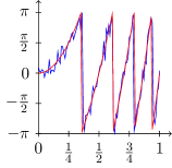
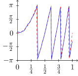
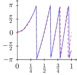
We start with the one-dimensional signal in Fig. 1 to show how the different functions from Table 1 perform and how the parameter influences the results. The original signal in Fig. 1 (a) was obtained from by sampling with size and unwrapping modulo such that the data are represented in . Then wrapped Gaussian noise with standard deviation was added. Using to restore the signal gives relatively larges error in Fig. 1 (b). The Huber function and the exponential function show better results in Fig. 1 (c) and 1 (d). The regularization parameter was adapted to get the best error
| (29) |
where . Making in the Huber function larger leads to the smoother result in Fig.1 (e) which approximates the original signal only well at the beginning of the signal. In Fig. 1 (f) we choose a larger in the function with the effect that edges of smaller height are smoothed and we have a staircasing effect for nearly equally high ascents.
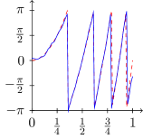
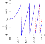
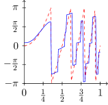
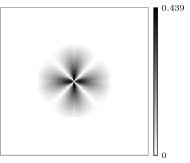
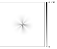
Next we want to demonstrate the difference between the anisotropic (15) and isotropic (16) half-quadratic minimization methods. To this end, the function was sampled over a regular grid with grid size , resulting in Fig. 2 (a). Then we corrupt the image by removing a circular region from the center as shown in Fig. 2 (d). Using the anisotropic functional leads to Fig. 2 (b), where we observe artifacts in vertical and horizontal directions. The image produced by applying the isotropic functional in Fig. 2 (c) does not have this problem. This effect is also illustrated by the error plots in Figs. 2 (e) and 2 (f).


4.2 -valued data
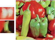
In our first example we denoise color images in the chromaticity and brightness space. For an RGB image the brightness is given by the real positive numbers and the chromaticity by the -values . We want to mention that the first two examples consider problems which have values on the positive octant; only in the last example we look at data covering the whole sphere. We compare half-quadratic minimization with the different functions and the TV approach from [56] in Fig. 3. We took the image “Peppers”222Taken from the USC-SIPI Image Database, available online at http://sipi.usc.edu/database/database.php?volume=misc&image=15 in Fig. 3 (a) and added Gaussian noise with standard deviation to all three color channels in the RGB model. For denoising in the chromaticity-brightness model we optimized with respect to best PSNR for both channels separately using a grid search on for and , and for on . Furthermore, we optimized first in order of magnitude and refined the search on . Both channels are restored using the same function. The square-root functional shows smoother transitions at edges while the Huber function tends more to staircasing. Using the exponential function yields a worse PSNR and hence does not compete with the previous two functions; the edges are preserved but within the more constant regions some noise is left. The bright spot (see upper magnification) appears also too smooth. This originates from the too smooth transitions in the brightness which are not detected as edges. The TV regularization introduces staircasing and it is not able to reduce the noise in the dark area (lower magnification).


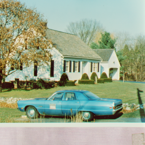
In the second example we use half-quadratic minimization for colorization in the chromaticity-brightness space. We assume that the brightness of the image is known, but 99 percent of the chromaticity information is lost. The original image is shown in Fig. 4 (a) and its corrupted version in Fig. 4 (b). For inpainting the chromaticity we have used a nearest neighbor initialization. With the regularizing function we obtain the result depicted in Fig. 4 (c). We compare this with Fig. 4 (d) which is obtained by using the chromaticity colorization method in [37] which we have implemented for comparison.

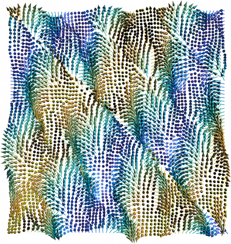
Our final experiment shows the smoothing of 3D directions in the synthetic image in Fig. 5 (b). We use half-quadratic minimization with to obtain Fig. 5 (c). The original pattern is again visible.
4.3 -valued data
Our first example illustrates the inpainting capabilities of the half-quadratic minimization method by an artificial example. The -valued image of size in Fig. 6 (a) has a jump at in direction. We destroy a center square of size , see Fig. 6 (b). We are able to reconstruct the inpainting area nearly perfectly by using and , see Fig. 6 (c). Nevertheless decreasing introduces more and more staircasing, cf. Fig. 6 (d). This resembles the TV case shown in Fig. 6 (e), using the model from [56].
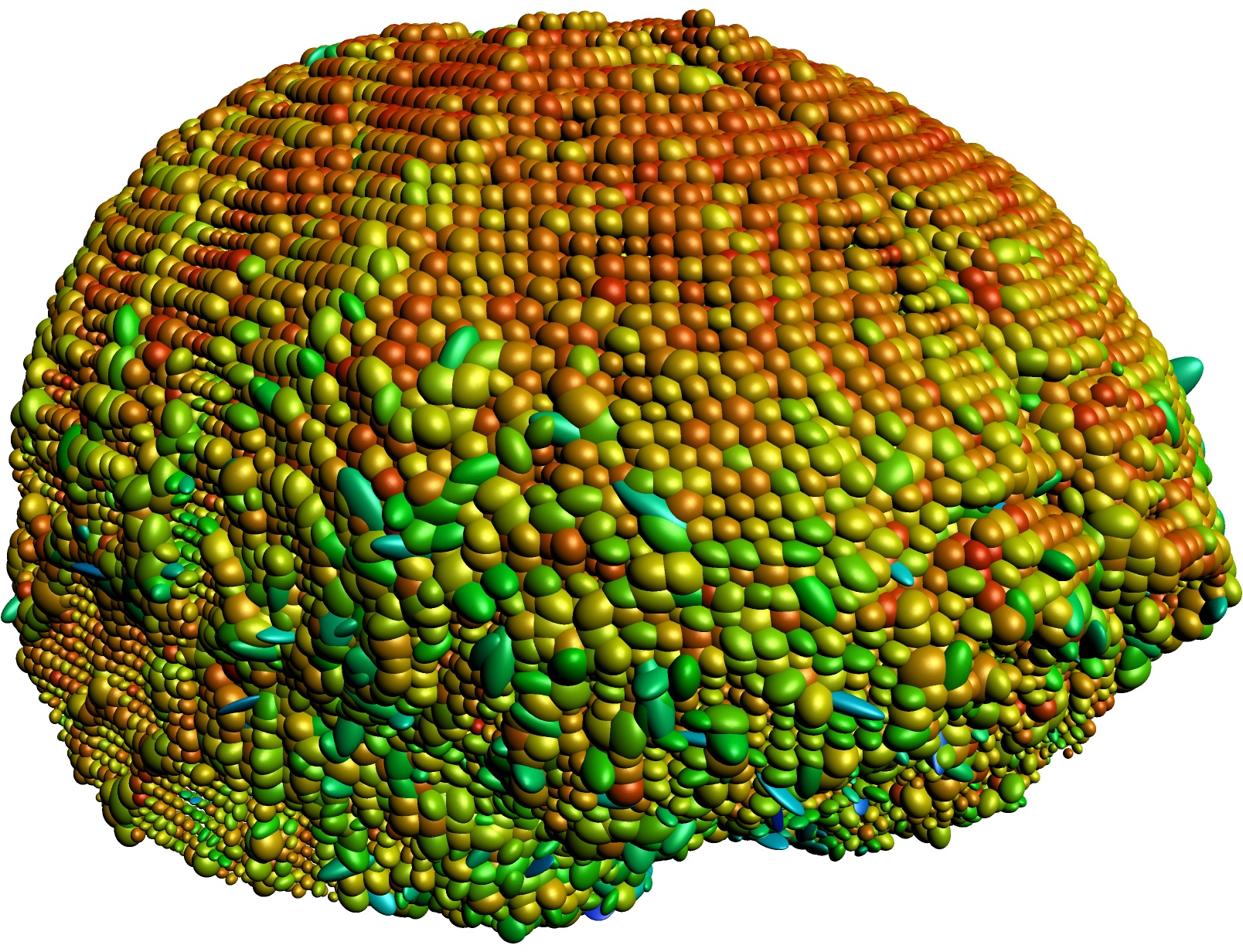
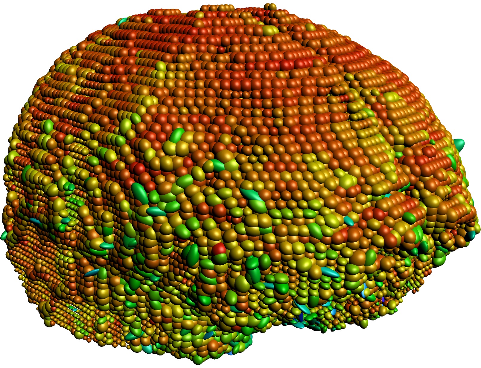
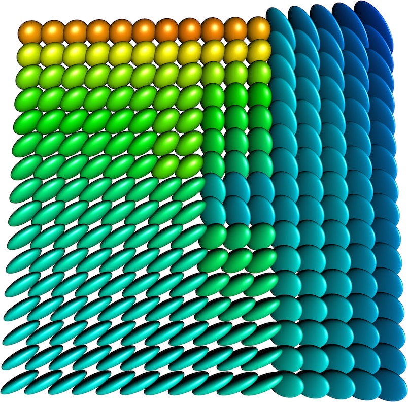
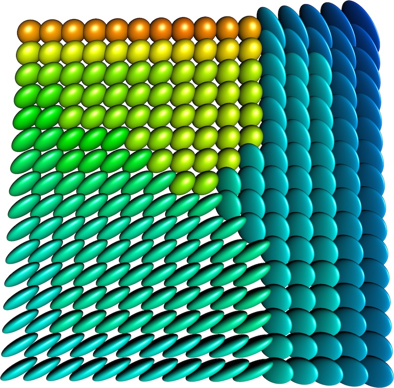
An important application of -valued image denoising is Diffusion Tensor Magnetic Resonance Imaging (DT-MRI). The Camino project333see http://cmic.cs.ucl.ac.uk/camino[17] provides a DT-MRI dataset of the human head which is freely available.444follow the tutorial at http://cmic.cs.ucl.ac.uk/camino//index.php?n=Tutorials.DTI The complete data is given as a 3D image , where we apply the half-quadratic minimization to each of the traversal planes . The original dataset, cf. Fig. 7 (a), is plotted using the anisotropy index relative to the Riemannian distance [32] normalized onto and colored in hue. The half-quadratic minimization is used with and the parameters , and a maximum change between two successive iterations being as a stopping criterion. We obtain the result shown in Fig. 7 (b). For the complete dataset of nonzero matrices, the algorithm needed seconds to compute the result.
4.4 -valued data
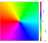
Processing images with -valued entries is fundamental in the analysis of polycrystalline materials by means of Electron Backscattered Diffraction (EBSD), cf. [28, 2]. Since the microscopic grain structure affects macroscopic attributes of materials such as ductility, electrical and lifetime properties, there is a growing interest in the grain structure of crystalline materials such as metals and minerals. EBSD provides us for each position on the surface of a specimen with a so called Kikuchi pattern, which allows the identification of the structure (material index) and the orientation of the crystal at this position relative to a fixed coordinate system ( value). Since the atomic structure of a crystal is invariant under its specific symmetry group the orientation is only given as an equivalence class , .
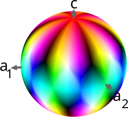
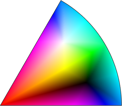
Fig. 8 (a) displays a typical EBSD image consisting of lattice orientations of deformed Magnesium collected by [43]. Each pixel of the image corresponds to a position on the surface of a Magnesium specimen. The color of the pixels is chosen corresponding to the orientation measured at this position according to the following color mapping: for a fixed vector we consider the mapping , . Next we colorize the quotient as it is depicted in Fig. 8 (b). From the colorization scheme the symmetry group of Magnesium becomes visible which has six rotations with respect to a 6-folded axis (, rotations around direction) and six rotations with respect to 2-folded axis , perpendicular to that.
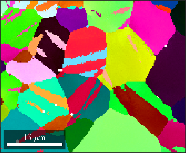
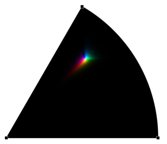
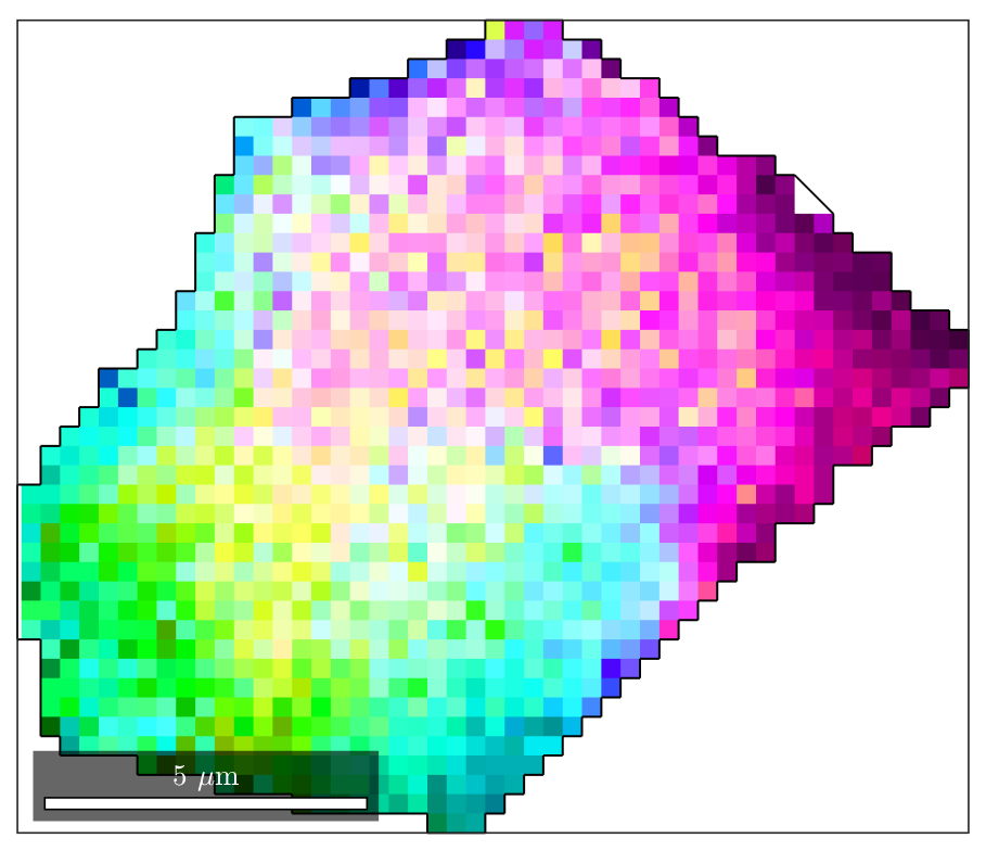
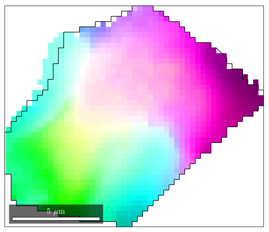
EBSD images usually consist of regions with similar orientations called grains. For certain macroscopic properties the pattern of orientations within single grains is of importance [7], e.g., for the computation of geometrically necessary dislocations [35, 49] the gradient of the rotations within single grains has to be determined. As the rotation determination by Kikuchi patterns is sometimes fragile, the rotation valued images determined by EBSD are often corrupted by noise and suffer from missing data so that denoising and inpainting techniques have to be applied [25]. For detecting grains in the raw EBSD data we applied a thresholding algorithm [8]. Fig. 9 (a) displays a single grain with its rotations. Since the rotations vary very little within a single grain we applied a sharper colorization, cf. Fig. 8 (d) to make the noise and the rotation gradient visible.
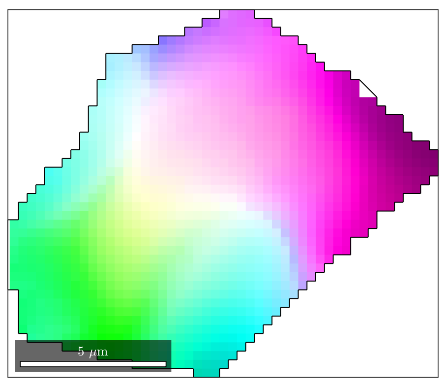
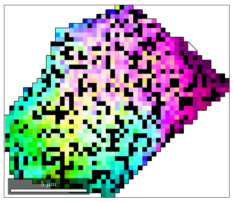
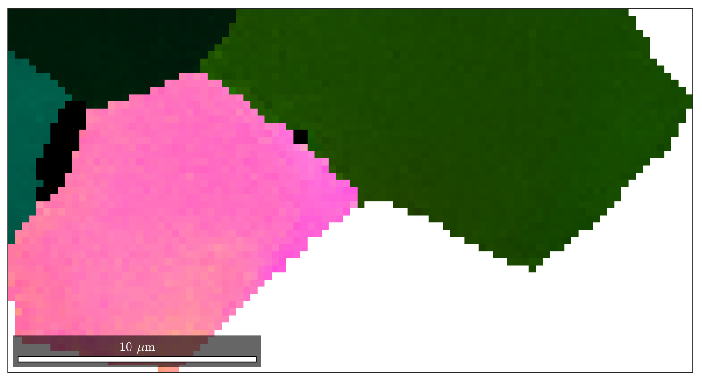
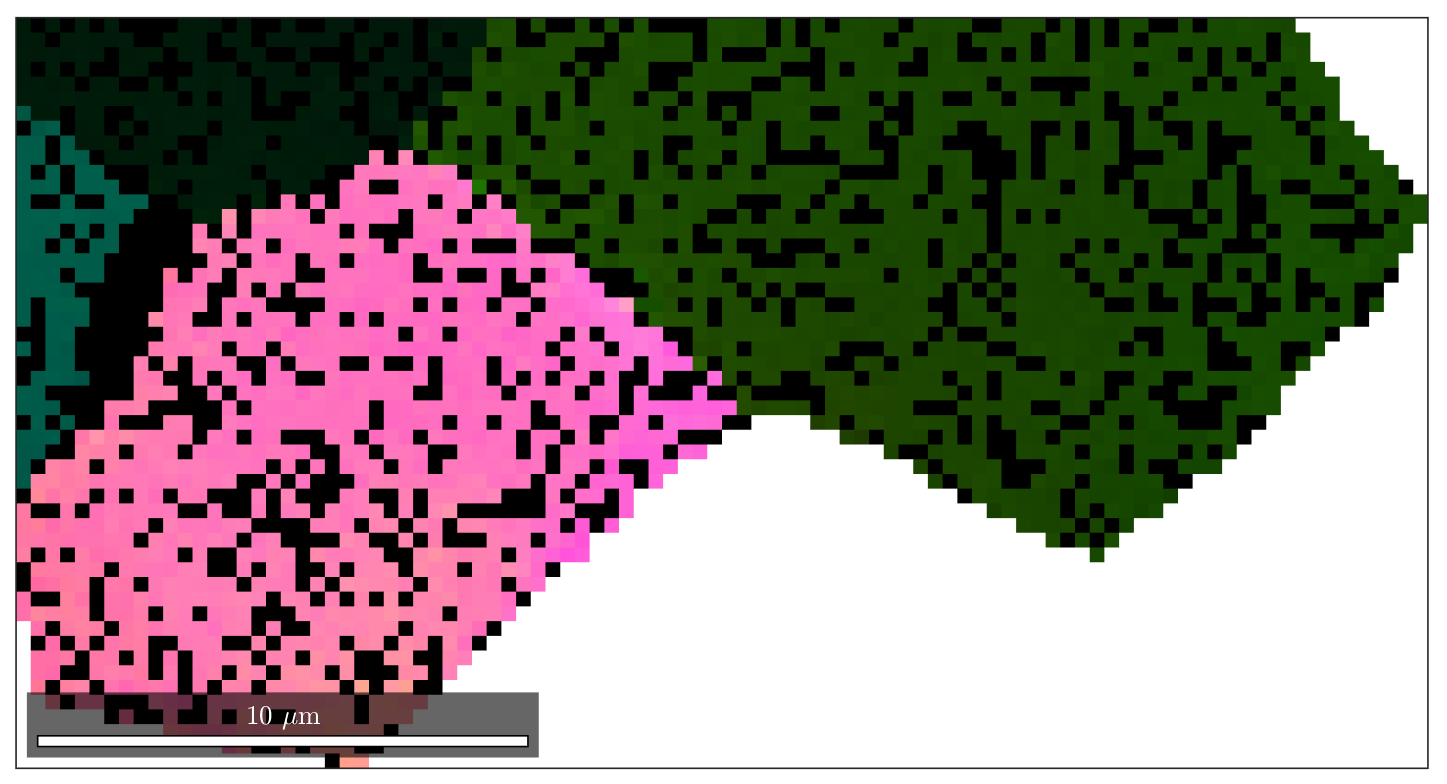
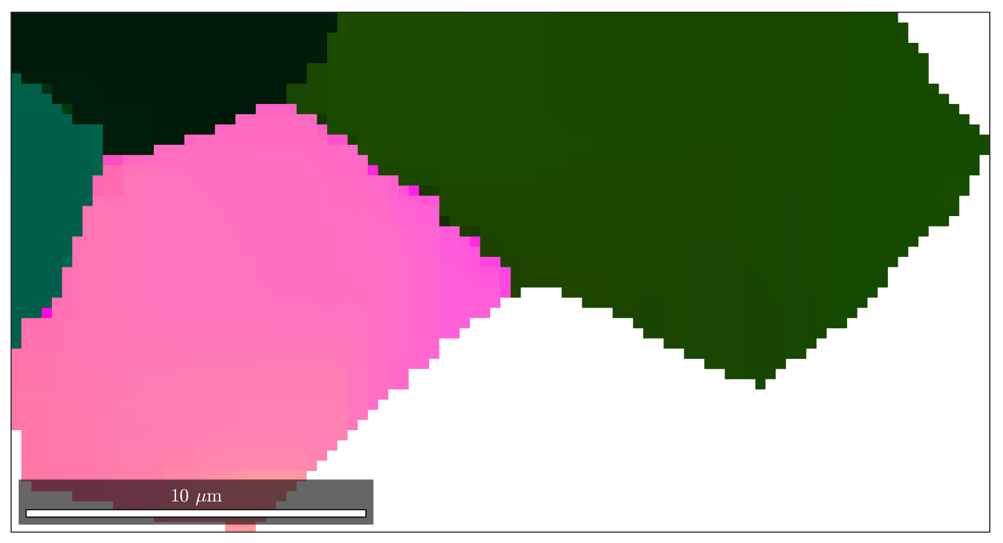
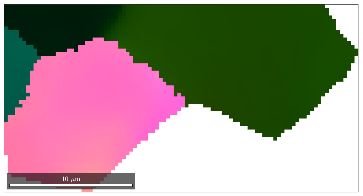
We want to apply half-quadratic minimization to denoise EBSD images. Since crystallographic symmetry groups are finite the quotient is locally isomorphic to . In particular, the formulas given in Appendix B.3 can be applied. In a first experiment we apply half-quadratic minimization using to the rotation-valued image depicted in Fig. 9 (a) which leads to the smooth image in Fig. 9 (b). In a second experiment we randomly removed of the data shown in Fig. 9 (c). Using half-quadratic minimization for jointly inpainting and denoising the image we obtain the result shown in Fig. 9 (d) which looks very similar to those in Fig. 9 (b). In a third experiment we applied half-quadratic minimization simultaneously to several grains. The challenge from the mathematical point of view is that is not an Hadamard manifold. Convergence can be guaranteed only locally, which is the case for single grains but may be not true when considering several grains simultaneously. From the practical point of view this case is especially interesting as missing data usually occur at grain boundaries, i.e., between grains. However, for our data we have got promising results. Fig. 10 (a) shows the grain from the previous example (pink color) and two other grains in its neighborhood. Note that the top middle area (light green) and top right area (brown-green) belong to the same grain. Pixels with missing data are plotted white. Half-quadratic minimization restoration with improves the image as can be seen in Fig. 10 (b). For our last experiment we again randomly remove of the data, cf. Fig 10 (c). Restoration with leads to the result in Fig. 10 (d), which is again hardly to distinguish from Fig. 10 (b). Using leads to even better results as depicted in Fig. 10 (e). We can adjust the smoothing in such a way that the edge distinguishing two grains is not smoothed, while smaller rotation changes are smoothed. This is advantageous in the large top grain. Finally Fig. 10 (f) shows the zoom to the (pink) grain from Fig. 9 with adapted color map.
5 Conclusions
We adapted the principles of half-quadratic minimization to the setting of complete, connected Riemannian manifolds. In particular, the notation of the -transform provides an interesting point of view. For Hadamard manifolds we proved the existence and uniqueness of the minimizer of the corresponding functionals as well as the convergence for the alternating minimization algorithm under moderate assumptions. The multiplicative half-quadratic minimization method resembles a quasi-Newton method [33] and appears to be very efficient in our numerical examples. There are numerous applications of the approach. In this paper, images having values in a manifold such as the 2-sphere or the symmetric positive definite matrices were denoised. The method was also used for inpainting missing information into images consisting of either rotation matrices or symmetric positive definite matrices. In the chromaticity-brightness color model, the inpainting technique was applied to the task of colorization. The method has further potential in EBSD.
Topics of future research are the derivation of convergence proofs for more general manifolds under special assumptions on the local behavior of the data. Furthermore, different data terms must be included for other applications, and the inclusion of higher order differences into the regularization term of the model is of interest.


Appendix A Proofs
Proof of Proposition 2.1..
1. In the additive case we have
By assumption on we know that which implies
This finishes the proof of i). The function
is continuous, convex and by (12) coercive so that the global minimizer in (9)
is attained for , i.e., for which proves ii).
2. In the multiplicative case we obtain, since is even,
We have
so that we can restrict our attention to . By assumption, is convex and lsc. Thus, and we obtain for that
This yields i). To see ii) we first note that condition (11) implies for that the objective function in (9) is coercive such that the infimum is attained. For , we have . For , we obtain
By assumption on , the function is convex in . A global minimizer of is attained either for the solution of if this solution is positive or for if , i.e., . Therefore is a solution.
Finally, the concavity of for implies that and thus is decreasing. Under the additional assumption in iii) we get . ∎
Proof of Proposition 3.3..
i) If , let , where . Then goes to infinity and the functionals , , are coercive. In the case choose and let be the constant image with entries . Let . Assume that remains finite, so that in particular and , , are finite. By the construction of the neighborhoods there exists for every a path with and
Since the right-hand side remains finite this contradicts .
Hence are coercive.
ii)
By (D2) we have that is convex and
strictly convex if .
If a function is convex, then,
for any geodesic joining , we obtain since
is increasing and convex that
| (30) |
so that is convex. If is strictly convex the last inequality is strong so that is strictly convex. With this implies by (D1) that is convex, resp. strictly convex. Concerning notice that the convexity of , , on implies convexity of on by
and by the Schwarz inequality
In the case , strict convexity follows by the strict convexity of the data term and for strictly convex by the strict convexity in (30). ∎
Proof of Theorem 3.4..
By Remark 3.1 we know that and that there exists a subsequence which converges to some . Since is continuous we have . Let
The continuity of and implies that and the continuity of that . By (27) we conclude
Thus, and since and have unique minimizers we obtain that and . Consequently, and , which by Remark 2.2 implies that is a minimizer of .
Assume that . Then there exists such that infinitely many not contained in the open ball of radius centered at . Since is bounded, there exists a convergent subsequence which converges to some point in the closed set . Then which contradicts the fact that has a unique minimizer. ∎
Appendix B Exponential and Logarithmic Maps
B.1 The Sphere
We use the parametrization
Then we have the tangent spaces
with the normed orthogonal vectors
The Riemannian metric is just the Euclidean distance in . The geodesic distance is given by , and the exponential map and (locally) its inverse, resp., by
| (31) | |||
| (32) |
B.2 The Manifold of Symmetric Positive Definite Matrices
By and we denote the matrix exponential and logarithm defined by
Let denote the space of symmetric matrices with (Frobenius) inner product and norm
| (33) |
Let be the manifold of symmetric positive definite matrices. It has the dimension . The tangent space of at is given by , in particular , where denotes the identity matrix. The Riemannian metric on reads
| (34) |
where denotes the matrix inner product (33). The geodesic distance is given by and the exponential map and its inverse by
see [44].
B.3 The Manifold of Rotation Matrices in
The manifold of rotation matrices is defined as
The geodesic distance between two rotation matrices is given by
The tangential space at reads
For the exponential map at and (locally) its inverse are defined as
The can be parametrized in various ways. Due to the form of our data we prefer to use quaternions for the representation and the similarity of to the group , see, e.g., [23]: We decompose the unit quaternions into a real part and a vector part . The multiplication of two quaternions is given by
with the conjugate quaternion as inverse element and unit element . The quaternions can be identified with the rotations of , where the quaternions and correspond to the same rotation. More precisely, is a double cover of , see, [12, Chap. III, Sect. 10]:
We work with the representative having a positive first component. With this representation at hand, he Riemannian metric of can be deduced from the Euclidean metric in . The geodesic distance can be written as
The exponential map of is given by
and the logarithmic map at of by
Acknowledgement: Funding by the DFG within the RTG GrK 1932 “Stochastic Models for Innovations in the Engineering Sciences”, project area P3, and in the projects STE 571/13-1 and BE 5888/2-1 is gratefully acknowledged. Furthermore RC gratefully acknowledges support by the HKRGC Grants No. CUHK300614, CUHK2/CRF/11G, AoE/M-05/12; CUHK DAG No. 4053007, and FIS Grant No. 1907303.
References
- [1] P.-A. Absil, R. Mahony, and R. Sepulchre. Optimization Algorithms on Matrix Manifolds. Princeton and Oxford, Princeton University Press, 2008.
- [2] B. L. Adams, S. I. Wright, and K. Kunze. Orientation imaging: The emergence of a new microscopy. Journal Metallurgical and Materials Transactions A, 24:819–831, 1993.
- [3] A. D. Aleksandrov. A theorem on triangles in a metric space and some of its applications. In Trudy Mat. Inst. Steklov., v 38, pages 5–23. Izdat. Akad. Nauk SSSR, Moscow, 1951.
- [4] M. Allain, J. Idier, and Y. Goussard. On global and local convergence of half-quadratic algorithms. IEEE Transactions on Image Processing, 15(5):1130–1142, 2006.
- [5] M. Bačák. Convex Analysis and Optimization in Hadamard Spaces, volume 22 of De Gruyter Series in Nonlinear Analysis and Applications. De Gruyter, Berlin, 2014.
- [6] M. Bačák, R. Bergmann, G. Steidl, and A. Weinmann. A second order non-smooth variational model for restoring manifold-valued images. Preprint Univ. Kaiserslautern, 2015.
- [7] F. Bachmann, R. Hielscher, P. E. Jupp, W. Pantleon, H. Schaeben, and E. Wegert. Inferential statistics of electron backscatter diffraction data from within individual crystalline grains. Journal of Applied Crystallography, 43:1338–1355, 2010.
- [8] F. Bachmann, R. Hielscher, and H. Schaeben. Grain detection from 2d and 3d EBSD data – specification of the MTEX algorithm. Ultramicroscopy, 111:1720–1733, 2011.
- [9] R. Bergmann, F. Laus, G. Steidl, and A. Weinmann. Second order differences of cyclic data and applications in variational denoising. SIAM Journal on Imaging Sciences, 7(4):2916–2953, 2014.
- [10] R. Bergmann and A. Weinmann. Inpainting of cyclic data using first and second order differences. In X.-C. Tai, E. Bai, T. Chan, S. Y. Leung, and M. Lysaker, editors, EMMCVPR2015, Lecture Notes in Computer Science, pages 155–168, Berlin, 2015. Springer.
- [11] R. Bergmann and A. Weinmann. A second order TV-type approach for inpainting and denoising higher dimensional combined cyclic and vector space data. ArXiv Preprint, 1501.02684, 2015.
- [12] G. E. Bredon. Topology and Geometry, volume 139 of Graduate Texts in Mathematics. Springer, New York, 1993.
- [13] R. Bürgmann, P. A. Rosen, and E. J. Fielding. Synthetic aperture radar interferometry to measure earth’s surface topography and its deformation. Annual Reviews Earth and Planetary Science, 28(1):169–209, 2000.
- [14] F. Champagnat and J. Idier. A connection between half-quadratic criteria and EM algorithms. IEEE Signal Processing Letters, 11(9):709–712, 2004.
- [15] T. F. Chan, S. Kang, and J. Shen. Total variation denoising and enhancement of color images based on the CB and HSV color models. Journal of Visual Communication and Image Representation, 12:422–435, 2001.
- [16] P. Charbonnier, L. Blanc-Féraud, G. Aubert, and M. Barlaud. Deterministic edge-preserving regularization in computed imaging. IEEE Transactions on Image Processing, 6(2):298–311, 1997.
- [17] P. A. Cook, Y. Bai, S. Nedjati-Gilani, K. K. Seunarine, M. G. Hall, G. J. Parker, and D. C. Alexander. Camino: Open-source diffusion-mri reconstruction and processing. In Proc. Intl. Soc. Mag. Reson. Med. 14, page 2759, Seattle, WA, USA, 2006.
- [18] I. Daubechies, R. DeVore, and C. S. Güntürk. Iteratively reweighted least squares minimization for sparse recovery. Communications in Pure and Applied Mathematics, 63(1):1–38, 2010.
- [19] A. H. Delaney and Y. Bresler. Globally convergent edge-preserving regularized reconstruction: an application to limited-angle tomography. IEEE Transactions on Image Processing, 7(2):204–221, 1998.
- [20] C.-A. Deledalle, L. Denis, and F. Tupin. NL-InSAR: Nonlocal interferogram estimation. IEEE Transactions on Geoscience Remote Sensing, 49(4):1441–1452, 2011.
- [21] D. Geman and G. Reynolds. Constrained restoration and the recovery of discontinuities. IEEE Transactions on Pattern Analysis and Machine Intelligence, 14(3):367–383, 1992.
- [22] D. Geman and C. Yang. Nonlinear image recovery with half-quadratic regularization. IEEE Transactions on Image Processing, 4(7):932–946, 1995.
- [23] M. Gräf. A unified approach to scattered data approximation on and . Advances in Computational Mathematics, 37:379–392, 2012.
- [24] P. Grohs and M. Sprecher. Total variation regularization by iteratively reweighted least squares on Hadamard spaces and the sphere. Preprint 2014-39, ETH Zürich, 2014.
- [25] V. K. Gupta and S. R. Agnew. A simple algorithm to eliminate ambiguities in EBSD orientation map visualization and analyses: Application to fatigue crack-tips/wakes in aluminum alloys. Microscopy and Microanalysis, 16:831, 2010.
- [26] J. Jost. Nonpositive Curvature: Geometric and Analytic Aspects. Lectures in Mathematics ETH Zürich. Birkhäuser Verlag, Basel, 1997.
- [27] R. Kimmel and N. Sochen. Orientation diffusion or how to comb a porcupine. Journal of Visual Communication and Image Representation, 13:238–248, 2002.
- [28] K. Kunze, S. I. Wright, B. L. Adams, and D. J. Dingley. Advances in automatic EBSP single orientation measurements. Textures and Microstructures, 20:41 – 54, 1993.
- [29] R. Lai and S. Osher. A splitting method for orthogonality constrained problems. Journal of Scientific Computing, 58(2):431–449, 2014.
- [30] C. L. Lawson. Contributions to the theory of linear least maximum approximation. Ph.D. Thesis, University of California, Los Angeles, 1961.
- [31] J. Lellmann, E. Strekalovskiy, S. Koetter, and D. Cremers. Total variation regularization for functions with values in a manifold. In IEEE ICCV 2013, pages 2944–2951, 2013.
- [32] M. Moakher and P. G. Batchelor. Symmetric positive-definite matrices: From geometry to applications and visualization. In J. Weickert and H. Hagen, editors, Visualization and Processing of Tensor Fields, pages 285–298. Springer Berlin Heidelberg, Berlin, Heidelberg, 2006.
- [33] M. Nikolova and R. H. Chan. The equivalence of half-quadratic minimization and the gradient linearization iteration. IEEE Transactions on Image Processing, 16(6):1623–1627, 2007.
- [34] M. Nikolova and M. K. Ng. Analysis of half-quadratic minimization methods for signal and image recovery. SIAM Journal on Scientific Computing, 27(3):937–966, 2005.
- [35] J. F. Nye. Some geometrical relations in dislocated crystals. Acta Mater., 1:153–162, 1953.
- [36] X. Pennec, P. Fillard, and N. Ayache. A Riemannian framework for tensor computing. International Journal of Computer Vision, 66:41–66, 2006.
- [37] M. H. Quang, S. H. Kang, and T. M. Le. Image and video colorization using vector-valued reproducing kernel Hilbert spaces. Journal of Mathematical Imaging and Vision, 37:49–65, 2010.
- [38] M. Raptis and S. Soatto. Tracklet descriptors for action modeling and video analysis. In ECCV 2010, pages 577–590. Springer, 2010.
- [39] J. G. Rešetnjak. Non-expansive maps in a space of curvature no greater than . Akademija Nauk SSSR. Sibirskoe Otdelenie. Sibirskiĭ Matematičeskiĭ Žurnal, 9:918–927, 1968.
- [40] G. Rosman, M. Bronstein, A. Bronstein, A. Wolf, and R. Kimmel. Group-valued regularization framework for motion segmentation of dynamic non-rigid shapes. In Scale Space and Variational Methods in Computer Vision, pages 725–736. Springer, 2012.
- [41] G. Rosman, X.-C. Tai, R. Kimmel, and A. M. Bruckstein. Augmented-Lagrangian regularization of manifold-valued maps. Methods and Applications of Analysis, 21(1):105–122, 2014.
- [42] L. I. Rudin, S. Osher, and E. Fatemi. Nonlinear total variation based noise removal algorithms. Physica D, 60(1):259–268, 1992.
- [43] Z.-Z. Shi and J.-S. Lecomte. private communication, 2014.
- [44] S. Sra and R. Hosseini. Conic geometric optimization on the manifold of positive definite matrices. ArXiv Preprint 1320.1039v3, 2014.
- [45] G. Steidl, S. Setzer, B. Popilka, and B. Burgeth. Restoration of matrix fields by second order cone programming. Computing, 81:161–178, 2007.
- [46] E. Strekalovskiy and D. Cremers. Total variation for cyclic structures: Convex relaxation and efficient minimization. In IEEE CVPR 2011, pages 1905–1911. IEEE, 2011.
- [47] E. Strekalovskiy and D. Cremers. Total cyclic variation and generalizations. Journal of Mathematical Imaging and Vision, 47(3):258–277, 2013.
- [48] K. T. Sturm. Probability measures on metric spaces of nonpositive curvature, heat kernels and analysis on manifolds, graphs, and metric spaces. Contemporary Mathematics, 338:357–390, 2003.
- [49] S. Sun, B. Adams, and W. King. Observation of lattice curvature near the interface of a deformed aluminium bicrystal. Phil. Mag. A, 80:9–25, 2000.
- [50] O. Tuzel, F. Porikli, and P. Meer. Learning on Lie groups for invariant detection and tracking. In CVPR 2008, pages 1–8. IEEE, 2008.
- [51] L. Vese and S. Osher. Numerical methods for p-harmonic flows and applications to image processing. SIAM Journal on Numerical Analysis, 40:2085–2104, 2002.
- [52] C. Villani. Topics in Optimal Transportation. AMS, Providence, 2003.
- [53] C. R. Vogel and M. E. Oman. Iterative method for total variation denoising. SIAM Journal on Scientific Computing, 17(1):474–477, 1996.
- [54] C. R. Vogel and M. E. Oman. Fast, robust total variation-based reconstruction of noisy, blurred images. IEEE Transactions on Image Processing, 7(6):813–824, 1998.
- [55] J. Weickert, C. Feddern, M. Welk, B. Burgeth, and T. Brox. PDEs for tensor image processing. In J. Weickert and H. Hagen, editors, Visualization and Processing of Tensor Fields, pages 399–414, Berlin, 2006. Springer.
- [56] A. Weinmann, L. Demaret, and M. Storath. Total variation regularization for manifold-valued data. SIAM Journal on Imaging Sciences, 7(4):2226–2257, 2014.
- [57] M. Welk, C. Feddern, B. Burgeth, and J. Weickert. Median filtering of tensor-valued images. In B. Michaelis and G. Krell, editors, Pattern Recognition, Lecture Notes in Computer Science, 2781, pages 17–24, Berlin, 2003. Springer.