Liquid-gas coexistence vs. energy minimization with respect to the density profile in the inhomogeneous inner crust of neutron stars

Abstract

We compare two approaches to describe the inner crust of neutron stars: on the one hand, the simple coexistence of a liquid (clusters) and a gas phase, and on the other hand, the energy minimization with respect to the density profile, including Coulomb and surface effects. We find that the phase-coexistence model gives a reasonable description of the densities in the clusters and in the gas, but the precision is not high enough to obtain the correct proton fraction at low baryon densities. We also discuss the surface tension and neutron skin obtained within the energy minimization.

I Introduction

The usual picture of the neutron-star crust Chamel and Haensel (2008) is that one starts from a Coulomb crystal of nuclei in the outer crust. As one goes deeper into the star, the nuclei become more and more neutron rich (as a consequence of the increasing electron chemical potential and $\beta$ equilibrium) until the neutron drip line is reached. This defines the transition to the inner crust, where the nuclei (“clusters”) are embedded in a dilute gas of unbound neutrons. Descending further into the star, one expects to find the so-called “pasta phases” Ravenhall et al. (1983); Hashimoto et al. (1984); Lassaut et al. (1987); Oyamatsu (1993); Watanabe et al. (2003); Napolitani et al. (2007); Avancini et al. (2008, 2010); Sebille et al. (2011); Baldo et al. (2014); Pais et al. (2014, 2015), before one finally reaches the neutron-star core where matter becomes homogeneous. The inhomogeneous phases in the inner crust can also be interpreted in another way Avancini et al. (2008), which is quite common in the study of supernova matter (i.e., matter at finite temperature and out of $\beta$ equilibrium) Pais et al. (2015); Aymard et al. (2014), namely as a consequence of the first-order liquid-gas instability of nuclear matter. One aim of the present paper is to see to what extent the simple picture of phase coexistence can explain certain properties of the inhomogeneous phases of the inner crust of neutron stars.

In particular, the phase coexistence picture corresponds to a hydrostatic equilibrium which can serve as a starting point for a hydrodynamic model of the collective modes in the inner crust Magierski (2004); Magierski and Bulgac (2004); Di Gallo et al. (2011). The collective modes can have some impact on thermodynamic and transport properties of the crust and may have observable consequences on the cooling of the star Page and Reddy (2012). While there exist several calculations of the collective modes in the crystalline phases Khan et al. (2005); Cirigliano et al. (2011); Chamel et al. (2013), it seems to be difficult to model the collective modes in the pasta phases beyond the hydrodynamic approach Di Gallo et al. (2011).

Within the most simple phase-coexistence picture, surface- and Coulomb energies are neglected. An approximate way to include them is the compressible liquid-drop model (see, e.g., Pais et al. (2015)). However, this model does not account for the neutron skin and for the effect of the surface diffuseness on the Coulomb energy. Therefore, we will use here a more microscopic approach, namely to parameterize the density profile and determine its parameters by minimizing the thermodynamic potential. Nevertheless it will turn out that the densities in the dense (“liquid”) and dilute (“gas”) regions satisfy quite well the conditions of phase coexistence.

The article is organized as follows. In Sec. II, we describe the formalisms for the phase coexistence and for the more complete minimization of the thermodynamic potential. In Sec. III, we show and compare the results obtained in both models, and in Sec. IV we conclude.

II Formalism

II.1 Phase coexistence

As a first approximation, the inner crust could be described as a phase coexistence of liquid drops (corresponding to the nuclear clusters) with volume $V^{\text{liq}}$ and a gas (the dilute neutron gas) with volume $V^{\text{gas}}$, which satisfies mechanical and chemical equilibrium, i.e.,

$$P^{\text{gas}} =P^{\text{liq}}\,,$$ (1)

$$\mu^{\text{gas}}_{q} =\mu^{\text{liq}}_{q}\,,$$ (2)

with $P^{i}$ the pressure, and $\mu_{q}^{i}$ the chemical potential of neutrons ($q=n$) or protons ($q=p$), respectively, in the phase $i$.

In addition to the neutrons and protons, we consider a uniform electron gas to ensure charge neutrality, i.e., $V\rho_{e}=V^{\text{liq}}\rho^{\text{liq}}_{p}+V^{\text{gas}}\rho^{\text{gas}}_{p}$, where $V=V^{\text{liq}}+V^{\text{gas}}$ is the total volume and $\rho_{p}^{i}$ is the proton density in phase $i$ ($\rho_{p}^{\text{gas}}$ is not always zero). Instead of working with the volumes, it is more convenient to introduce the volume fraction $u$ filled by the liquid, which satisfies

$$u=\frac{V^{\text{liq}}}{V}=\frac{\rho_{e}-\rho_{p}^{\text{gas}}}{\rho_{p}^{\text{liq}}-\rho_{p}^{\text{gas}}}\,.$$ (3)

Furthermore, in neutron stars, matter is in $\beta$ equilibrium, i.e.,

$$\mu_{e}=\mu_{n}-\mu_{p}\,$$ (4)

with $\mu_{e}$ the chemical potential of the electrons. For practical purposes, the electron mass can be neglected so that $\mu_{e}=(3\pi^{2}\rho_{e})^{1/3}\hbar c$. We thus obtain for the volume fraction

$$u=\frac{1}{\rho_{p}^{\text{liq}}-\rho_{p}^{\text{gas}}}\left[\frac{(\mu_{n}-\mu_{p})^{3}}{3\pi^{2}(\hbar c)^{3}}-\rho_{p}^{\text{gas}}\right]\,.$$ (5)

We use a Skyrme energy-density functional (EDF) Chabanat et al. (1997) to calculate the energy density $\epsilon_{\text{Sk}}$ as a function of $\rho_{n}$ and $\rho_{p}$. This allows us to write explicit expressions for the chemical potentials $\mu_{q}=\partial\epsilon_{\text{Sk}}/\partial\rho_{q}$ and the pressure $P=-\epsilon_{\text{Sk}}+\mu_{n}\rho_{n}+\mu_{p}\rho_{p}$ appearing in Eqs. (2) and (1). We use different Skyrme parametrizations, all fitted to the neutron-matter equation of state: the Saclay-Lyon forces SLy4 and SLy7 Chabanat et al. (1998) and the Brussels-Montreal forces BSk20 and BSk22 Goriely et al. (2013).

II.2 Energy minimization

In the phase-coexistence picture described above, we could determine the volume fraction $u$, but not the actual size of the clusters. The latter is determined by finding the best compromise between the Coulomb energy (favoring small clusters) and the surface energy (favoring large clusters), which were both neglected in the phase-coexistence picture. Let us now consider a more sophisticated approach, where these effects are included.

The surface energy is computed within the semiclassical Extended Thomas-Fermi (ETF) approximation Brack et al. (1985); Aymard et al. (2014). Instead of solving Euler-Lagrange equation Lassaut et al. (1987); Baldo et al. (2014), we use a parametrization of the density profile and determine the parameters by minimizing the energy. Concerning the Coulomb energy, we use the Wigner-Seitz (WS) approximation, i.e., we calculate the Coulomb energy in an isolated cell $r<R_{\text{WS}}$, with $R_{\text{WS}}$ chosen such that the volume of the WS cell corresponds to the volume of the unit cell. Inside the WS cell, our density is parametrized as

$$\rho_{q}(r)=\rho_{q}^{\text{gas}}+\frac{\rho_{q}^{\text{liq}}-\rho_{q}^{\text{gas}}}{1+\exp\left[(r-r_{q})/a_{q}\right]}$$ (6)

and the energy is minimized with respect to the 9 parameters $\rho_{q}^{i}$, $r_{q}$, $a_{q}$, and $R_{\text{WS}}$. This parametrization looks similar to the shape obtained in Hartree-Fock calculation, e.g., LABEL:Negele1973 and has a simple interpretation: $\rho_{q}^{\text{liq}}$ and $\rho_{q}^{\text{gas}}$ correspond, respectively, to the asymptotic densities in the cluster and in the gas far away from the surface, $r_{q}$ describes the cluster radius, including the possibility of a neutron skin if $r_{n}>r_{p}$, and $a_{q}$ is the surface diffuseness. We also tried a more general parametrization using two more parameters, namely, raising the Fermi function in Eq. (6) to a power $\gamma_{q}$. This additional degree of freedom allows one to describe an “asymmetric” surface, but since it did not substantially change our results we discarded it for simplicity.

Note that a similar approach was followed by Oyamatsu Oyamatsu (1993) and by Pearson et al. Pearson et al. (2012). However, Oyamatsu used a completely different parametrization of the density, which did not become constant inside the cluster. Our parametrization (6) resembles more the one used by Pearson et al.

It seems very hard to perform the minimization of the energy for fixed average densities (averaged over the WS cell), since the average densities depend on all the parameters. We therefore introduce chemical potentials $\mu_{q}$ as Lagrange parameters to fix the densities and minimize the thermodynamic potential instead of the energy. To be precise, we minimize $\omega=-P=\Omega/V_{\text{WS}}$, where

$$\Omega=E_{\text{Sk}}-\mu_{n}N-\mu_{p}Z-\mu_{e}Z+E_{e}+E_{C}+E_{\text{ex}}\,,$$ (7)

which reduces to

$$\Omega=E_{\text{Sk}}-\mu_{n}(N+Z)+E_{e}+E_{C}+E_{\text{ex}}\,,$$ (8)

because of the $\beta$-equilibrium constraint (4). In this equation, $E_{\text{Sk}}$ denotes the energy obtained with the Skyrme functional, $N$ and $Z$ are the total numbers of neutrons and protons in the WS cell, $E_{e}$ denotes the energy of the electron gas, $E_{C}$ the Coulomb energy, and $E_{\text{ex}}$ the energy due to the Coulomb exchange term.

The volume $V_{\text{WS}}$ of the WS cell depends on $R_{\text{WS}}$ and on the geometry one considers (spheres, rods, or slabs). Let us define the functions $S_{d}(r)$ and $V_{d}(r)$ describing, respectively, the “surface” and the “volume” of a $d$ dimensional sphere of radius $r$, i.e.,

$$S_{1}(r) =2\,, S_{2}(r) =2\pi r\,, S_{3}(r) =4\pi r^{2}\,,$$ (9)

$$V_{1}(r) =2r\,, V_{2}(r) =\pi r^{2}\,, V_{3}(r) =\tfrac{4}{3}\pi r^{3}\,.$$ (10)

In the case of spheres ($d=3$), the volume of the WS cell is $V_{\text{WS}}=V_{3}(R_{\text{WS}})$. In the case of rods ($d=2$), the “volume” $V_{\text{WS}}=V_{2}(R_{\text{WS}})$ is actually an area and consequently $E$, $N$, $Z$, etc. represent energies and particle numbers per unit length. Similarly, in the case of slabs ($d=1$), the “volume” $V_{\text{WS}}=V_{1}(R_{\text{WS}})$ is a length and $E$, $N$, $Z$, etc. represent energies and particle numbers per unit area.

The integrated Skyrme energy in the WS cell, $E_{\text{Sk}}$, is defined as

$$E_{\text{Sk}}=\int_{0}^{R_{\text{WS}}}d^{d}r\,\mathcal{H}[\rho_{n}(r),\rho_{p}(r)]\,,$$ (11)

with $d^{d}r=S_{d}(r)dr$ and $\mathcal{H}$ the Skyrme EDF detailed in LABEL:Chabanat1997, the kinetic energy density $\tau_{q}(r)$ being calculated within the ETF approximation as described in Brack et al. (1985); Aymard et al. (2014).

For the energy of the electron gas, we assume a constant density $\rho_{e}=Z/V_{\text{WS}}$. Hence, the energy can be written as $E_{e}=V_{\text{WS}}\epsilon_{e}$. The energy density $\epsilon_{e}$, taking into account the electron mass $m_{e}$, reads Baldo et al. (2014)

$$\epsilon_{e}=\frac{\hbar ck_{F,e}^{4}}{4\pi^{2}}\left[\left(1+\frac{1}{2x_{e}^{2}}\right)\sqrt{1+\frac{1}{x_{e}^{2}}}-\frac{\sinh^{-1}x_{e}}{2x_{e}^{4}}\right]\,,$$ (12)

with $k_{F,e}=(3\pi^{2}\rho_{e})^{1/3}$ and $x_{e}=\hbar k_{F,e}/m_{e}c$.

The Coulomb energy $E_{C}$ is derived from the charge density $\rho_{c}(r)=\rho_{p}(r)-\rho_{e}$. We first calculate the Coulomb potential $V_{C}(r)$ satisfying the Poisson equation $\operatorname{\nabla^{2}}V_{C}(r)=4\pi e^{2}\rho_{c}(r)$ with $\operatorname{\bm{\nabla}}V_{C}(0)=0$. This determines $V_{C}(r)$ only up to a constant, which is however irrelevant for the energy since the total charge of the WS cell is zero. The Coulomb energy is given by

$$E_{C}=\frac{1}{2}\int_{0}^{R_{\text{WS}}}d^{d}r\rho_{c}(r)V(r)\,.$$ (13)

Note that $V_{C}(r)$ and the integral (13) must be computed numerically, in contrast to the approximate expressions one obtains for uniformly charged spheres (or rods, or slabs, respectively) with a sharp surface which are often used in the literature Ravenhall et al. (1983); Hashimoto et al. (1984); Avancini et al. (2010); Pais et al. (2014).

We relaxed the assumption of a constant electron density by using a screened Coulomb potential instead of the full one, i.e., replacing in the Poisson equation $\operatorname{\nabla^{2}}V_{C}(r)$ by ($\operatorname{\nabla^{2}}-1/\lambda^{2})V_{C}(r)$, where $\lambda$ denotes the Debye screening length, $1/\lambda^{2}=(4\alpha/\pi)k_{Fe}^{2}$ (neglecting the electron mass), with $\alpha=e^{2}/\hbar c$. However, as already noticed in Maruyama et al. (2005), the screening length of the electrons is so large that this effect is negligible and the calculations of the present paper were done without electron screening.

The exchange term of the Coulomb interaction is computed within the Slater approximation Baldo et al. (2014). For the protons, it is given by the integral of

$$\epsilon_{\text{ex},p}(r)=-\frac{3}{4}\left(\frac{3}{\pi}\right)^{1/3}e^{2}\rho_{p}^{4/3}(r)\,,$$ (14)

over the WS cell. For the relativistic electrons, the exchange energy includes also contributions from transverse photons and gets positive for $x_{e}\gtrsim 2.53$ Salpeter (1961). Its expression reads Rajagopal (1978)

$$\epsilon_{\text{ex},e}=\frac{e^{2}k_{F,e}^{4}}{8\pi^{3}}\left\{3\left[\sqrt{1+\frac{1}{x_{e}^{2}}}-\frac{\sinh^{-1}x_{e}}{x_{e}^{2}}\right]^{2}-2\right\}\,,$$ (15)

III Results

III.1 Phase coexistence

Let us first discuss the results obtained within the simple phase coexistence approach. Figure 1

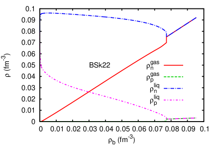
Figure 1: (Color online) Neutron and proton densities in the coexisting liquid (droplets) and gas phases, calculated with the Skyrme parametrization BSk22.

represents the densities in the gas and in the liquid as functions of the baryon density

$$\rho_{b}=u(\rho_{n}^{\text{liq}}+\rho_{p}^{\text{liq}})+(1-u)(\rho_{n}^{\text{gas}}+\rho_{p}^{\text{gas}})\,,$$ (16)

obtained with the BSk22 interaction Goriely et al. (2013). Results calculated with other Skyrme parametrizations are close to those displayed for BSk22 (cf. Fig. 5 for SLy4). The main difference is the transition to uniform matter, i.e., the point where the liquid fills the whole volume ($u=1$). For instance, the transition occurs at $\rho_{b}\approx 0.09~{}\text{fm}^{-3}$ with SLy4, while with BSk22 it is below $0.08~{}\text{fm}^{-3}$.

Figure 2

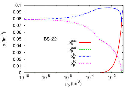
Figure 2: (Color online) Same as Fig. 1 but with a logarithmic scale for the baryon density.

shows the same results, but on a logarithmic scale so that the low density region is better visible. The region below $\rho_{b}\approx 10^{-3}~{}\text{fm}^{-3}$ corresponds to the outer crust, where $\rho^{\text{gas}}_{n}=\rho^{\text{gas}}_{p}=0$ (i.e., $\mu_{n},\mu_{p}\leq 0$). In the limit of extremely low densities, the droplets are made of symmetric nuclear matter at saturation density ($\rho_{n}=\rho_{p}=0.08$ fm^-3). The kink in the densities visible in Fig. 2 corresponds to the transition between the outer and the inner crust, i.e., to the point where $\mu_{n}$ becomes positive and the neutron gas appears.

Close to the transition to uniform matter, also $\mu_{p}$ becomes positive and the gas phase does not only contain neutrons, but also a small amount of protons. Figure 3

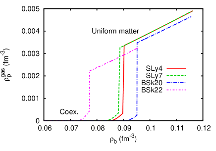
Figure 3: (Color online) Proton density in the gas phase (and later in uniform matter) as function of the total baryon density calculated within the phase coexistence approach using the SLy4, SLy7, BSk20 and BSk22 Skyrme parametrizations.

zooms on densities where protons are present in the gas. Note that the proton density in the gas is always very low, less than $10^{-3}~{}\text{fm}^{-3}$ for all Skyrme parametrizations, compared to the other densities calculated in the phase coexistence framework.

III.2 Energy minimization

In the preceding subsection, we treated the inner crust as two nuclear fluids in phase coexistence. As already mentioned in Sec. II.2, this approach misses surface and Coulomb effects, which are included in the minimization of the thermodynamic potential with respect to the parameters of the density profile given in Eq. (6). Actually, we perform the minimization for each of the three different geometries discussed in Sec. II.2, namely spheres (3D), rods (2D), and slabs (1D). The geometry giving the lowest thermodynamic potential should be the one that is physically realized.

From now on, we restrict ourselves to the range $\mu_{n}>0$ corresponding to the inner crust and show the results as functions of the average baryon density $\rho_{b}=A/V_{\text{WS}}$, where $A=N+Z$ is the total number of nucleons in the WS cell. Figure 4

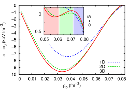
Figure 4: (Color online) The thermodynamic potential $\omega$ as function of the baryon density $\rho_{b}$, with the thermodynamic potential $\omega_{u}$ of uniform matter subtracted. In the inset, a phenomenological function $\overline{\omega}$ is subtracted, which approximates the average behavior of the three $\omega$’s. The SLy4 interaction was used in this calculation.

displays the difference $\omega-\omega_{u}$ between the thermodynamic potentials $\omega$ in 3D, 2D, and 1D geometry, obtained by numerical minimization with the SLy4 interaction, and the thermodynamic potential $\omega_{u}$ of uniform $npe$ matter in $\beta$ equilibrium with the same baryon density. The difference is negative, confirming that the inhomogeneous phase is favored over uniform matter in this density range. In order to make the differences between the 3D, 2D, and 1D geometries better visible, we subtract in the inset a purely phenomenological function $\bar{\omega}$ which approximates the average behavior of the three $\omega$’s. At densities below $0.061~{}\text{fm}^{-3}$, the most favorable phase is the crystal (3D). From $0.061$ to $0.073~{}\text{fm}^{-3}$ the preferred phase are the rods (“spaghetti”, 2D). Finally between $0.073$ and $0.081~{}\text{fm}^{-3}$ we find the slabs (“lasagne”, 1D), until the system transforms into uniform matter. In contrast to other work Ravenhall et al. (1983); Hashimoto et al. (1984); Lassaut et al. (1987); Oyamatsu (1993); Pais et al. (2014, 2015), we did not find “inverted” geometries such as tubes and bubbles (“Swiss cheese”), which would correspond to $\rho_{q}^{\text{gas}}>\rho_{q}^{\text{liq}}$ in the parametrization (6) of the density profile in 2D and 3D, respectively.

Let us note that the energy differences between the three geometries are extremely small compared to the total energy, especially between 2D and 3D beyond $\sim 0.05~{}\text{fm}^{-3}$, so that one may expect coexistence of different geometries. This is because, in contrast to most studies of the pasta phases, we do not consider a fixed proton fraction, but $\beta$ equilibrium. As pointed out in LABEL:Piekarewicz2012, the small proton fraction (see below) corresponding to $\beta$ equilibrium is very unfavorable for the formation of pasta phases. Our method results necessarily in first-order phase transitions between the different geometries. In reality, however, it might happen that the system passes continuously from one phase to another, e.g., by deforming the nuclei in the 3D phase before they merge into rods Ravenhall et al. (1983); Lattimer and Swesty (1991).

The densities $\rho_{q}^{i}$ in the favored geometry obtained by the minimization are displayed in Fig. 5 as the solid lines.

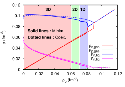
Figure 5: (Color online) Solid lines: densities in the cluster ($\rho_{q}^{\text{liq}}$) and in the gas ($\rho_{q}^{\text{gas}}$) corresponding to the geometry (3D, 2D, 1D, or uniform matter) that minimizes $\omega$ in Fig. 4, obtained by the minimization of the SLy4 functional. Dots: results obtained within the phase coexistence approach as in Fig. 1 but with the SLy4 interaction.

We notice a discontinuity at the transition from 2D to 1D. It is due to the first-order phase transition mentioned above (the corresponding jump between 3D to 2D is too small to be seen on the figure). For comparison, the dotted lines in Fig. 5 were calculated as in Fig. 1 within the phase coexistence framework. The densities obtained within both approaches are quite similar, which means that even with Coulomb and surface effects, the mechanical and chemical equilibrium, Eqs. (1) and (2), are approximately satisfied for the densities in the cluster and in the gas away from the interface. The main difference is the transition density from the inner crust to uniform matter, i.e., to the neutron star core. Since Coulomb and surface effects favor uniform matter, the transition happens earlier (i.e., at lower $\rho_{b}$) in the minimization than in the phase coexistence approach.

Although the differences in the densities are small, they have a sizable effect on the proton fraction $Y_{p}=Z/A$. This can be seen in Fig. 6,

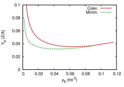
Figure 6: (Color online) Proton fraction $Y_{p}$ as function of the baryon density $\rho_{b}$. The proton fraction is computed using the SLy4 interaction with the phase coexistence (solid line) and the energy minimization (dots) approach.

where we compare the proton fractions obtained within the phase coexistence approach (solid lines) and by energy minimization (dots). It appears that at low baryon density, the proton fraction obtained by minimizing the energy is significantly lower than in the phase coexistence picture, although the proton densities in the liquid are very close (cf. Fig. 5). A very similar difference between the two approaches is observed in the Relativistic Mean-Field (RMF) framework Avancini et al. (2008). This disagreement can be traced back to the tiny difference in $\rho_{n}^{\text{gas}}$ due to the small Coulomb and surface corrections to the chemical and mechanical equilibrium. Since in this region the total density is dominated by the density of the gas, $\rho_{b}\approx\rho_{n}^{\text{gas}}$, and the volume fraction $u$ is approximately proportional to the difference $\rho_{B}-\rho_{n}^{\text{gas}}$, the quantities $u$ and consequently also $Y_{p}$ are very sensitive to small deviations of $\rho_{n}^{\text{gas}}$.

The proton fractions obtained by energy minimization are similar to those obtained by Pearson et al. Pearson et al. (2014) within the Hartree-Fock-Bogoliubov (HFB) model with BSk interactions. However, in contrast to the HFB model, the ETF approximation does not include shell effects. Therefore, our proton number in the 3D phase varies smoothly from $Z\approx 34$ at low baryon density to $Z\approx 26$ at the transition to the 2D phase, while the HFB model gives $Z=40$ in the whole inner crust except in the case of the BSk22 interaction where $Z$ jumps from 40 to 20 at $\rho_{b}=0.035$ fm^-3 Pearson et al. (2014).

III.3 Properties of the liquid-gas interface

Let us discuss in some more detail the properties of the liquid-gas interface obtained by energy minimization. To that end, we have to compare our WS cell with a reference system containing a cluster with constant densities $\rho_{q}^{\text{liq}}$ and a sharp surface, surrounded by a gas with constant densities $\rho_{q}^{\text{gas}}$. The presence of a neutron skin $s_{n}=r_{n}-r_{p}>0$ complicates this comparison, and we follow Douchin and Haensel Douchin et al. (2000) who discussed this problem in detail.

We define the radius $r_{p}^{\text{eff}}$ of the reference cluster in such a way that it contains the same number of protons as the actual WS cell, i.e.,

$$(\rho_{p}^{\text{liq}}-\rho_{p}^{\text{gas}})V_{d}(r_{p}^{\text{eff}})+\rho_{p}^{\text{gas}}V_{\text{WS}}=Z\,$$ (17)

($\rho_{p}^{\text{gas}}=0$ in most cases, except near the crust-core transition, cf. Fig. 5). Note that $r_{p}^{\text{eff}}$ coincides with $r_{p}$ in the case $d=1$, but not in the cases $d=2$ or $3$. If we used an asymmetric surface (see discussion below Eq. (6)), $r_{p}^{\text{eff}}$ would differ from $r_{p}$ also in the case $d=1$.

Since we define the reference cluster with a common surface at $r_{p}^{\text{eff}}$ for protons and neutrons, i.e., without neutron skin, the reference system contains less neutrons than the actual WS cell. Therefore, rather than comparing the energies of two systems having different numbers of particles, one should compare their thermodynamic potentials. The surface contribution to the thermodynamic potential, $\Omega_{s}$, is defined as the change in $\Omega$ (excluding Coulomb) with respect to the “bulk” thermodynamic potential (i.e., excluding gradient terms) of the reference cluster. We denote $V^{\text{liq}}=V_{d}(r_{p}^{\text{eff}})$ the volume of the reference cluster and $V^{\text{gas}}=V_{\text{WS}}-V^{\text{liq}}$ the volume of the surrounding gas. Then the surface potential can be written as

$$\Omega_{s}= E_{\text{Sk}}-\mu_{n}N-\mu_{p}Z$$

$$-V^{\text{liq}}(\epsilon_{\text{Sk}}^{\text{liq}}-\mu_{n}\rho_{n}^{\text{liq}}-\mu_{p}\rho_{p}^{\text{liq}})$$

$$-V^{\text{gas}}(\epsilon_{\text{Sk}}^{\text{gas}}-\mu_{n}\rho_{n}^{\text{gas}}-\mu_{p}\rho_{p}^{\text{gas}})\,,$$ (18)

where $\epsilon_{\text{Sk}}^{i}$ is the energy density obtained with the Skyrme functional $\cal{H}$ in the case of uniform matter with densities $\rho_{n}^{i}$ and $\rho_{p}^{i}$.

Analogously to Eq. (17), we define an effective neutron radius $r_{n}^{\text{eff}}$, and an effective volume of the neutron skin $V_{s}=V_{d}(r_{n}^{\text{eff}})-V_{d}(r_{p}^{\text{eff}})$. Then the number of neutrons in the skin, $N_{s}$, is given by

$$N_{s}=V_{s}(\rho_{n}^{\text{liq}}-\rho_{n}^{\text{gas}})\,,$$ (19)

and Eq. (18) can be rewritten as

$$\Omega_{s}=E_{\text{Sk}}-V^{\text{liq}}\epsilon_{\text{Sk}}^{\text{liq}}-V^{\text{gas}}\epsilon_{\text{Sk}}^{\text{gas}}-\mu_{n}N_{s}\,.$$ (20)

Finally, the surface energy $E_{s}$ is given by $E_{s}=\Omega_{s}+\mu_{n}N_{s}$ Douchin et al. (2000).

The surface tension is approximately given by $\sigma=\Omega_{s}/S_{d}(r_{p}^{\text{eff}})$, where $S_{d}(r)$ is defined in Eq. (9). Although $V_{d}(r)$ and $S_{d}(r)$ have the dimensions of a volume and of an area only in the case $d=3$, the ratio $\Omega_{s}/S_{d}(r_{p}^{\text{eff}})$ is always an energy per area. Note that the above definition of the surface tension is only exact in 1D or if the cluster radius is so large that curvature effects can be neglected. In Fig. 7

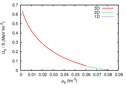
Figure 7: (Color online) The surface tension $\sigma$ as a function of the baryon density $\rho_{b}$. For each $\rho_{b}$, the result corresponding to the most favored geometry is displayed.

we display the surface tension. We see that it decreases with increasing $\rho_{b}$. This is not surprising because with increasing $\rho_{b}$ the densities in the gas and in the liquid get closer to each other. In the low-density limit, where we have essentially isolated nuclei, our surface tension is consistent with the surface energy in the Bethe-Weizsäcker semi-empirical mass formula from which one obtains $\sigma=1.03$ MeV fm^-2 Ring and Schuck (1980). Our surface tension is similar to the RMF results shown in Fig. 6(c) of Avancini et al. (2008).

Another interesting quantity is the number of additional neutrons in the skin. Again, we normalize it to the surface and display in Fig. 8

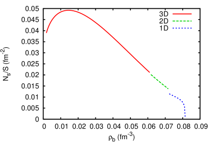
Figure 8: (Color online) The number of the additional neutrons due to the skin, $N_{s}$, divided by the cluster surface $S_{d}(r_{p}^{\text{eff}})$.

the number of skin neutrons per unit surface, $N_{s}/S_{d}(r_{p}^{\text{eff}})$. We observe that, after a maximum at $\rho_{b}\sim 0.014~{}\text{fm}^{-3}$, the number of neutrons in the skin decreases with increasing baryon density, although the skin thickness remains about $s_{n}\sim 0.45~{}\text{fm}$, because the density difference $\rho_{n}^{\text{liq}}-\rho_{n}^{\text{gas}}$ decreases. Note that, compared to the total number of neutrons in the WS cell, the number of neutrons in the skin is very small: for instance, for $\rho_{b}=0.02~{}\text{fm}^{-3}$ there are about $800$ neutrons in the cell, $200$ in the cluster, and only $23$ in the skin.

IV Conclusions

In our work we compared the results obtained for the inner crust within a simple phase-coexistence picture with results of the minimization of the energy with respect to the density profile. We used Skyrme interactions and the ETF approximation to calculate the energy. Both approaches give similar results for the neutron and proton densities in the clusters and in the gas, despite the Coulomb and surface effects included in the minimization but not in the phase coexistence.

However the phase-coexistence picture is insufficient to predict the cluster sizes and transitions between different geometries, since these result from the competition of Coulomb and surface energies not included in the phase coexistence. With increasing baryon density, we find crystals, rods and plates, but no “inverted” geometries such as tubes and bubbles. Because of the small proton fraction in $\beta$ equilibrium, the energy differences between the different geometries are extremely small. Another effect of Coulomb and surface energies is to shift the crust-core transition to lower baryon density.

Although the densities obtained by energy minimization do not present strong deviations from those of the phase coexistence, the proton fraction does, especially at low baryon densities. The small corrections to mechanical and chemical equilibrium due to Coulomb and surface effects slightly modify the density of the neutron gas, resulting in a considerable reduction of volume and proton fractions. The proton fractions obtained within the minimization are similar to HFB results in the literature Pearson et al. (2014), although shell effects, which are present in HFB, are missing in the ETF approximation to the energy.

The minimization allowed us to calculate the surface tension and the number of skin neutrons in the cluster surface. We plan to use these results in an improved hydrodynamic description of collective modes in the inner crust similar to the one of LABEL:DiGallo2011 but including Coulomb and surface effects.

References

- Chamel and Haensel (2008) N. Chamel and P. Haensel, Living Reviews in Relativity 11, 10 (2008).
- Ravenhall et al. (1983) D. G. Ravenhall, C. J. Pethick, and J. R. Wilson, Phys. Rev. Lett. 50, 2066 (1983).
- Hashimoto et al. (1984) M.-a. Hashimoto, H. Seki, and M. Yamada, Prog. Theor. Phys. 71, 320 (1984).
- Lassaut et al. (1987) M. Lassaut, H. Flocard, P. Bonche, P. Heenen, and E. Suraud, Astron. Astrophys. 198, L3 (1987).
- Oyamatsu (1993) K. Oyamatsu, Nucl. Phys. A 561, 431 (1993).
- Watanabe et al. (2003) G. Watanabe, K. Sato, K. Yasuoka, and T. Ebisuzaki, Phys. Rev. C 68, 035806 (2003).
- Napolitani et al. (2007) P. Napolitani, P. Chomaz, F. Gulminelli, and K. H. O. Hasnaoui, Phys. Rev. Lett. 98, 131102 (2007).
- Avancini et al. (2008) S. S. Avancini, D. P. Menezes, M. D. Alloy, J. R. Marinelli, M. M. W. Moraes, and C. Providência, Phys. Rev. C 78, 015802 (2008).
- Avancini et al. (2010) S. S. Avancini, S. Chiacchiera, D. P. Menezes, and C. Providência, Phys. Rev. C 82, 055807 (2010).
- Sebille et al. (2011) F. Sebille, V. de la Mota, and S. Figerou, Phys. Rev. C 84, 055801 (2011).
- Baldo et al. (2014) M. Baldo, G. Burgio, M. Centelles, B. Sharma, and X. Viñas, Yad. Fiz. [Sov. J. Nucl. Phys.] 77, 1157 (2014).
- Pais et al. (2014) H. Pais, W. G. Newton, and J. R. Stone, Phys. Rev. C 90, 065802 (2014).
- Pais et al. (2015) H. Pais, S. Chiacchiera, and C. Providência, arXiv e-print (2015), arXiv:1504.03964 [nucl-th] .
- Aymard et al. (2014) F. Aymard, F. Gulminelli, and J. Margueron, Phys. Rev. C 89, 065807 (2014).
- Magierski (2004) P. Magierski, Int. J. Mod. Phys. E 13, 371 (2004).
- Magierski and Bulgac (2004) P. Magierski and A. Bulgac, Acta Phys. Polon. B 35, 1203 (2004).
- Di Gallo et al. (2011) L. Di Gallo, M. Oertel, and M. Urban, Phys. Rev. C 84, 045801 (2011).
- Page and Reddy (2012) D. Page and S. Reddy, “Neutron star crust,” (Nova Science Publishers, Hauppauge, 2012) Chap. 14.
- Khan et al. (2005) E. Khan, N. Sandulescu, and N. V. Giai, Phys. Rev. C 71, 042801 (2005).
- Cirigliano et al. (2011) V. Cirigliano, S. Reddy, and R. Sharma, Phys. Rev. C 84, 045809 (2011).
- Chamel et al. (2013) N. Chamel, D. Page, and S. Reddy, Phys. Rev. C 87, 035803 (2013).
- Chabanat et al. (1997) E. Chabanat, P. Bonche, P. Haensel, J. Meyer, and R. Schaeffer, Nucl. Phys. A 627, 710 (1997).
- Chabanat et al. (1998) E. Chabanat, P. Bonche, P. Haensel, J. Meyer, and R. Schaeffer, Nucl. Phys. A 635, 231 (1998).
- Goriely et al. (2013) S. Goriely, N. Chamel, and J. M. Pearson, Phys. Rev. C 88, 024308 (2013).
- Brack et al. (1985) M. Brack, C. Guet, and H.-B. Håkansson, Phys. Rep. 123, 275 (1985).
- Negele and Vautherin (1973) J. Negele and D. Vautherin, Nucl. Phys. A 207, 298 (1973).
- Pearson et al. (2012) J. M. Pearson, N. Chamel, S. Goriely, and C. Ducoin, Phys. Rev. C 85, 065803 (2012).
- Maruyama et al. (2005) T. Maruyama, T. Tatsumi, D. N. Voskresensky, T. Tanigawa, and S. Chiba, Phys. Rev. C 72, 015802 (2005).
- Salpeter (1961) E. Salpeter, Astrophys. J. , 669 (1961).
- Rajagopal (1978) A. K. Rajagopal, J. Phys. C 11 (1978).
- Piekarewicz and Sánchez (2012) J. Piekarewicz and G. T. Sánchez, Phys. Rev. C 85, 015807 (2012).
- Lattimer and Swesty (1991) J. M. Lattimer and F. D. Swesty, Nucl. Phys. A 535, 331 (1991).
- Pearson et al. (2014) J. Pearson, N. Chamel, A. Fantina, and S. Goriely, Eur. Phys. J. A 50, 43 (2014).
- Douchin et al. (2000) F. Douchin, P. Haensel, and J. Meyer, Nucl. Phys. A 665, 419 (2000).
- Ring and Schuck (1980) P. Ring and P. Schuck, The Nuclear Many-Body Problem (Springer, Berlin, 1980).