A Comparison of Limit Setting Methods for the On-Off Problem

Abstract

We study the frequentist properties of confidence intervals found with various methods previously proposed for the On-Off problem. We derive explicit formulas for the limits and calculate the true coverage and the expected lengths of these methods.

1 Introduction

In this paper we study a problem called “On-Off ” in astrophysics and the problem of “one signal band and one sideband ” in high energy physics (HEP). In the astrophysics version, one points the telescope at ( “On ” ) a potential point signal source and observes $x$ counts in a particular amount of observing time. Then one points the telescope away from ( “Off ” ) the source to a nearby region thought to have no point sources, and observes $y$ counts in an observing time that is $\tau$ times as long as the “On ” observing time. The latter provides an estimate of the non-point-source rate $b$, which crudely speaking allows for a “background subtraction ”  in the on-source data. One desires a confidence interval for the point source rate $\mu$ in the presence of the background rate that can be inferred (with some uncertainty) only from $y$. Complications arise because, for weak sources and small counts $x$ and $y$, the Poisson-distributed data is not suitable for trivial formulas coming from Gaussian assumptions. So the probability model we are studying is given by

$$X\sim Pois(\mu+b)\text{ \ \ }Y\sim Pois(\tau b)$$ (1)

The same probability model arises if the background rate was estimated via Monte Carlo, in which case $\tau$ is related to the number of Monte Carlo runs.

Statistical Inference for this problem has a long history in HEP and Astronomy. It received renewed interest in 1997 by Feldman and Cousins [8], who applied their now famous Unified method to the case of a known background rate $b$. A general method for including an uncertainty into the model was proposed by Cousins and Highland [5] and was applied to the “On-Off ”  in Conrad et.al. [4] and Tegenfeldt and Conrad [17].

A solution based on inverting the likelihood ratio test was proposed by Rolke and Lopez [15] and extended to include uncertainty in the efficiency as well as other probability models for $Y$ by Rolke, Lopez and Conrad [16]. This is also known as profile likelihood method, which has a long history in Statistics and has been in use for a some time in physics in the MINUIT program when errors are calculated with the MINOS method, see James and Roos [11] and Li and Ma [12]. The class TRolke implements this method in ROOT, see Lundberg et.al. [13].

A different approach known as the CLs method was described by Read [14], and Gan and Kass [9] used the Cousins-Highland prescription to include uncertainties in the background rate into CLs. This solution is different from the others discussed in this paper in that it calculates upper limits only. Finally a number of intervals derived via the Bayesian paradigm have been proposed as well.

The problem of significance testing for the signal rate was studied by Cousins, Linnemann and Tucker [6], and in principle hypothesis testing and interval estimation are the same problem, as one can always invert a hypothesis test into an interval procedure and vice versa. In practice this can be difficult, and in fact the method favored by Cousins, Linneman and Tucker, namely turning the problem into one for a Binomial parameter p, can not be inverted into a limit setting method because it is specific to the test $H_{0}:\mu=0$. What is missing from the literature is a detailed study of the commonly used methods for limit setting in terms of their coverage as well as other properties, and it is this study we are undertaking in this paper.

The software tools commonly used to calculate these limits, for example RooStats, are general purpose tools that allow for much more complicated probability models, for example multiple channels, uncertainties in the detection efficiencies etc. Such generality comes at a price as these tools use Monte Carlo simulation for the limit calculations. This leads to two problems for our study: on the one hand the limits come with errors, often on the order of 5-10%, and it is not clear how one would determine the correct coverage in this case. Moreover, these tools are fairly slow in calculating the limits. This is not an issue if just one or even a few limits are needed. We, though, need a very large number of them: our study focuses on the small sample case, and so we restrict ourselves to $\mu\in[0,20]$ and $b\in[0,10]$. We also want to study a number of different $\tau$ values, say $\tau\in\{0.5,1,2\}$. With these parameters possible observations for which we need the limits range from $x=0$ to $x=50$ and the same for $y$. Also we want to study coverage at the nominal $68\%$, $90\%$ and $95\%$ levels. This means we need to calculate a total of $23409$ limits for each method. Obviously this requires a very fast way to find the limits, and in the next section we are developing exact formulas to be able to do so. Unfortunately this task becomes hopeless if we tried to incorporate further uncertainties, for example in $\tau$, into the models.

It should be noted that all results in this paper are based on exact calculations. They therefore do not carry with them any uncertainties due to a finite number of simulation runs.

2 The Methods

2.1 Intervals based on Inverting a Likelihood Ratio Test: Rolke-Lopez-Conrad (RLC)

Maybe the most widespread technique for deriving a hypothesis test in Statistics is the likelihood ratio test (LRT). Say we have a probability model $f(\mathbf{x};\theta)$ and we wish to test $H_{0}:$ $\theta\in\Theta_{0}$ vs $H_{a}:$ $\theta\notin\Theta_{0}$. Then the LRT is a test based on the test statistic

$$T(\mathbf{x)=}\frac{\sup_{\Theta_{0}}f(\mathbf{x};\theta)}{\sup_{\Theta}f(\mathbf{x};\theta)}$$ (2)

where $\Theta_{0}$ is some subset of the parameter space $\Theta$.

The reason for the popularity of this approach is two-fold: first by the famous Neyman-Pearson lemma it is known that in the case of a simple vs. simple hypothesis this test is optimal, that is has the highest possible power for a given type I error probability $\alpha$. Even though optimality is not guaranteed in more complicated cases, experience has shown that tests (and intervals) derived with this method tend to do very well. Also, under some regularity conditions in the large sample limit $-2\log T(\mathbf{x)}$ has a chi-square distribution. This is known as Wilk’s theorem, and a proof can be found in many Statistics text books, for example in Casella and Berger [3].

For our probability model we have

$$f(x,y;\mu,b)=\frac{(\mu+b)^{x}}{x!}e^{-(\mu+b)}\frac{(\tau b)^{y}}{y!}e^{-\tau b}$$ (3)

so $\theta=(\mu,b)$. Here and in what follows $\tau$ is considered a known constant. We want a confidence interval for $\mu$ alone, so we test $H_{0}:$ $\mu=\mu_{0}$ vs $H_{a}:\mu\neq\mu_{0}$. For the denominator of  $T$  we need to find the maximum likelihood estimators (mle), which are $\widehat{\mu}=x-y/\tau$ and $\widehat{b}=y/\tau$. For the numerator we need to maximize $f(x,y;\mu,b)$ for $b$ alone, treating $\mu$ as fixed. This leads to

$$\widehat{\widehat{b}}=\frac{x+y-(1+\tau)\mu+\sqrt{(x+y-(1+\tau)\mu)^{2}+4(1+\tau)y\mu}}{2(1+\tau)}$$ (4)

and then the test can be based on

$$-2\log T(x,y\mathbf{)=}2\left(\log f(x,y;\widehat{\mu},\widehat{b})-\log f(x,y;\mu_{0},\widehat{\widehat{b}})\right)$$ (5)

Replacing a nuisance parameter by the value that maximizes the likelihood function while keeping the parameter of interest fixed is known as the profile likelihood method and has a long history in Statistics.

Unfortunately in our case, at least when $\mu_{0}=0$, the regularity conditions of Wilk’s theorem are not satisfied. Moreover, we are far from a large-sample regime, and so the question arises as to what the null distribution might be. This was studied by Rolke and Lopez [15] who showed that the chi-square approximation is surprisingly good, and that confidence intervals derived by inverting the likelihood ratio test and using the chi-square approximation have good coverage properties, at least when some ad-hoc adjustments are made in the cases where the observed number of events in the signal region is less than what is expected from background alone. The $RLC$ method is implemented in the Root class Trolke, described in Lundberg et.al. [13].

2.2 Feldman-Cousins Unified Method

In 1997 Feldman and Cousins [8] proposed a limit setting method for the model $X\sim Pois(\mu+b)$ where $b$ is assumed known. The method proceeds as follows. Consider the Poisson density

$$f(x;\mu)=\frac{\mu^{x}}{x!}e^{-\mu}$$ (6)

where $x=0,1,..$ and $\mu\geq 0$. Now for all possible observations $x$ and a signal rate $\mu$ calculate the ratio

$$\frac{f(x;\mu+b)}{f(x;\widehat{\mu}+b)}$$ (7)

where $\widehat{\mu}=\max\{0,x-b\}$ is the maximum likelihood estimator (mle) of $\mu$. Rank the possible observations $x$ according to these ratios, resulting in the sequence $x_{i}^{\ast},i=1,2..$ Define the “acceptance region ” $A(\mu)$ by

$$A(\mu)=\left\{(x_{1}^{\ast},..,x_{n}^{\ast});\sum_{i=1}^{n}f(x_{i}^{\ast};\mu+b)\leq cl,\sum_{i=1}^{n+1}f(x_{i}^{\ast};\mu+b)>cl\right\}$$ (8)

where $cl$ is the desired confidence level, for example $0.95$ for a $95\%$ confidence interval. In the Statistics literature this methodology for deriving a test (and a corresponding limits method) is called the Neyman construction. The confidence interval for $\mu$ is comprised of all values of $\mu$ such that $A(\mu)$ includes the observed $x$. Because in the problem studied here this method leads to a simple interval this last step can be done by finding the endpoints.

It should be noted that in this case of a Poisson rate with a known background the limits found by the Feldman-Cousins method can also be derived by inverting the corresponding likelihood ratio test.

How can we extend this method to our more general problem? We will consider four options:

2.2.1 Feldman-Cousins Confidence Regions (FCR)

The most obvious solution is to consider confidence regions in $(\mu,b)$ space. So now we have pairs of points $(x,y)$ and again we find their Poisson probabilities

$$f(x,y;\mu,b)=\frac{(\mu+b)^{x}}{x!}e^{-(\mu+b)}\frac{(\tau b)^{y}}{y!}e^{-\tau b}$$ (9)

We find the maximum likelihood estimators $\widehat{\mu}=\max\{0,x-y/\tau\}$ and $\widehat{b}=y/\tau$, and calculate the ratios

$$\frac{f(x,y;\mu,b)}{f(x,y;\widehat{\mu},\widehat{b})}$$ (10)

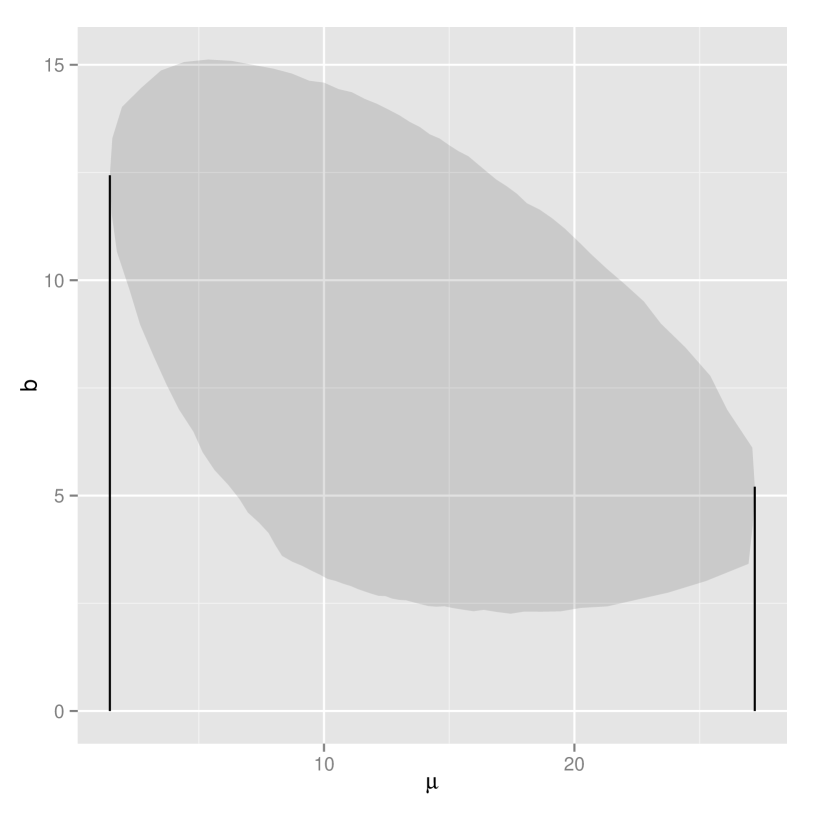
Figure 1: 2 dimensional $95\%$ confidence region for $(\mu,b)$ if $x=20,y=7$ and $\tau=1.0$. A $95\%$ confidence interval for $\mu$ is found by projecting region onto $\mu$ axis

Then we rank the points according to this ratio and “accept ” all points up to the desired confidence level. Then we scan through $(\mu,b)$ space to find the confidence region. As an example consider figure 1 which shows the $95\%$ confidence region for the case $x=20$, $y=7$ and $\tau=1$.

Of course $b$ is a nuisance parameter, and what we really want is a confidence interval for $\mu$. We can get that by projecting the region down onto the $\mu$-axis, but it is clear that such a method will suffer from over-coverage. Unfortunately no general method is known to extract a confidence interval from a confidence region in such a way that the confidence interval has correct coverage.

2.2.2 Feldman-Cousins Profile Likelihood (FCPL)

Because we are only interested in $\mu$ we can try to eliminate the background rate $b$ at some point during the calculations. One way to do this is to use the idea of profile likelihood already described above. Here when calculating the probabilities we replace the density $f(x,y;\mu,b)$ by $f_{PL}(x,y;\mu)$ defined by $f_{PL}(x,y;\mu)=f(x,y;\mu,\widehat{\widehat{b}})$, where $\widehat{\widehat{b}}$ is as in equation 4. Now the method proceeds exactly as the basic Feldman-Cousins method described above, except using $f_{PL}$ instead of $f$.

One problem with this approach is that $f_{PL}$ is no longer a probability density, in fact $\sum_{x,y}f_{PL}(x,y;\mu)=\infty$. So we need to restrict our calculations to $0\leq x\leq M_{x}$ and $0\leq y\leq M_{y}$ with $M_{x}$ and $M_{y}$ large enough so that their choice does not effect the limits significantly. In the numerical studies shown below we always use $M_{x}=M_{y}=50$, which we verified is large enough so that the effect on the limits is negligible. Moreover we need to normalize $f_{PL\text{ }}$so it is a proper probability density with

$$\sum_{x=0}^{M_{x}}\sum_{y=0}^{M_{y}}f_{PL}(x,y;\mu)=1$$ (11)

2.2.3 Cousins-Highland

Another way to eliminate $b$ is to use a procedure first advocated by Cousins and Highland [5]. The idea is to eliminate a nusiance parameter by integrating it out. There are essentially two ways to do this:

Feldman-Cousins-Cousins-Highland Option 1 (FCCH1)

Here we replace the probability density $f(x,y;\mu,b)$ with

$$f_{CH}(x,y;\mu):=\int_{0}^{\infty}f(x,y;\mu,b)db=$$

(12)

where we made use of the fact that

$$\int_{0}^{\infty}t^{k}e^{-at}dt=\frac{\Gamma(k+1)}{a^{k+1}}$$ (13)

which in turn follows because the integrand is the density of a Gamma distribution with parameters $k+1$ and $a$. $\Gamma$ denotes the gamma function.

Now limits are found the same way as before. Again we have the problem that $\sum_{x,y}f_{CH}(x,y;\mu)=\infty$, and we proceed as in section $2.2.2$. The normalized probabilities will be denoted by $f_{CH}^{*}$.

Feldman-Cousins-Cousins-Highland Option 2 (FCCH2)

In this version one first calculates limits $L(x;b)$ and $U(x;b)$ for the signal rate $\mu$ using the method of Feldman and Cousins for fixed background rate $b$, and then finds limits

$$L(x,y)=\int_{0}^{\infty}L(x;b)\tau\frac{(\tau b)^{y}}{y!}e^{-\tau b}db$$

(14)

essentially weighting each limit by the corresponding Poisson probabilities. The extra factor $\tau$ comes from the normalization $\int_{0}^{\infty}\frac{(\tau b)^{y}}{y!}e^{-\tau b}db=\frac{1}{\tau}$.

2.2.4 Neyman Construction with Probability Ordering (NeyProb)

There is yet another variation of this method: instead of using the likelihood ratio as the ordering principle we can simply use the probabilities $f_{CH}^{\ast}$. One of the reasons Feldman and Cousins did not use this ordering was that it can lead to empty intervals. For example if we have $\tau=1$, observe $x=0,y=6$ and want to find $95\%$ limits there is no $\mu\geq 0$ that will have the point $(0,6)$ in the acceptance region. If this is deemed acceptable, or if it is known a priori that there will be more events in the signal region than are expected from background alone, this is a viable method.

2.3 CLs

A method that has been used extensively in HEP is the CLs method. Here in the case of a known background rate $b$ one uses the test statistic

$$\frac{P(X\leq x|\mu+b)}{P(X\leq x|b)}$$ (15)

which means one is testing specifically $H_{0}:$ $\mu=0$ vs $H_{a}:\mu>0$. Therefore this method always yields upper limits.

CLs was first proposed in a special case by Zech [18] and generalized by Read [14]. Even though it has very little grounding in Statistical theory it has become quite popular in HEP. The extension to our “On-Off ” model was done by Gan and Kass [9], who used the Cousins-Highland prescription to show that an upper limit can be found by inverting a test based on the test statistic

$$T_{CLs}(\mu;x,y,\tau)=\frac{e^{-\mu}}{y!}\frac{\sum_{n=0}^{x}\sum_{k=0}^{n}\mu^{n-k}\binom{y+k}{y}/(n-k)!/(1+\tau)^{k}}{\sum_{n=0}^{x}\binom{y+k}{y}/(1+\tau)^{k}}$$ (16)

and the (say) $95\%$ upper limit is found by solving $T_{CLs}(\mu;x,y,\tau)=0.95$. The derivation of equation 16 is very similar to the calculations done for $f_{CH}$.

2.3.1 Bayesian Methods

The last class of methods we will consider are intervals derived using the Bayesian approach. Although we will find proper Bayesian credible intervals these will then be evaluated as standard frequentist confidence intervals. Helene [10] used a Bayesian approach to calculate limits for the “On-Off ” problem, although they modeled the background as a Gaussian rather than a Poisson.

As always in Bayesian Statistics we need to choose priors for $\mu$ and $b$. We will consider the following cases: flat priors, a fairly common choice in HEP, and Jeffrey’s non-informative prior, which in the case of a Poisson distribution with rate $\mu$ is given by $\pi(\mu)=1/\sqrt{\mu}$. We will consider all combinations of these priors. Lastly we will include another choice occasionally found in the literature, namely $\pi(\mu,b)=\frac{1}{\sqrt{\mu+b}}$. This is Jeffreys prior when $b$ is a known constant.

The last case does not allow for an analytic solution, and limits are found through numerical integration. For the first four we can handle all cases in one calculation by assuming priors of the form $\pi(\lambda)=\lambda^{-\rho}$, where $\rho=0$ or $1/2$.  With this we have the probability model

$$X\sim Pois(\mu+b)$$,   

,  

(17)

we begin by finding the marginal distribution of $x$ and $y$:

$$m(x,y)=\int_{0}^{\infty}\int_{0}^{\infty}f(x,y;\mu,b)\pi(b)\pi(\mu)d\mu db=$$

(18)

Next we find the posterior density of $\mu$ as the marginal of the joint posterior density:

$$f(\mu|x,y)=\int_{0}^{\infty}f(\mu,b|x,y)db=$$

(19)

We also need the posterior distribution function $F(\mu|x,y)$:

$$F(\mu|x,y)=\int_{0}^{\mu}f(t|x,y)dt=$$

(20)

where $F_{\Gamma}(.;\alpha,\beta)$ is the distribution function of a Gamma random variable with parameters $(\alpha,\beta)$.

Now we need to extract an interval from the posterior distribution. We will use the method of highest posterior density, which is the solution of the system of equations

$$f(L|x,y)=f(U|x,y)$$

(21)

The advantage of this solution over the more common equal tail area solution is that this method yields a smooth transition from one sided to two sided intervals and therefore avoids the problem of flip-flopping, which is further discussed in the section on Performance.

In the following we will denote the Bayesian methods by their priors, so for example $\pi(\mu,b)=1$ is the method with flat priors on both $\mu$ and $b$, $\pi(\mu,b)=1/\sqrt{\mu}$ uses Jeffrey’s prior on $\mu$ and a flat prior on $b$ etc.

3 Performance of these Methods

3.1
Coverage

The coverage $Cov$ of a set of confidence intervals $[L(x,y),U(x,y)]$ is defined by

$$Cov(\mu,b)=P\left(L(X,Y)\leq\mu\leq U(X,Y)|\mu,b\right)=$$

(22)

where $I_{A}(x)$ is the indicator function of the set  $A$ and $f(x,y;\mu,b)$ is the probability density from equation 3.

A $(1-\alpha)100\%$ confidence interval is said to have coverage if for all $(\mu,b)\in[0,\infty)\times[0,\infty)$

$$Cov(\mu,b)\geq 1-\alpha$$ (23)

For this paper we will restrict ourselves to the region of parameter space with $(\mu,b)\in[0,20]\times[0,10]$, relevant for counting experiments with low statistics. In the case of larger values of $\mu$ and $b$ one would likely use some asymptotic methods as studied by Cowan et.al. [7].

The experimenter might on occasion decide ahead of time that they will only calculate an upper limit, for example if theory suggests that the signal rate is very small or even $0$. The distinction between upper limits and two-sided confidence intervals is somewhat artificial because an upper limit can always be viewed as a confidence interval with $L(x,y)=-\infty$ for all $x,y$. Moreover the property of coverage applies equally to both. One important point, though, is that for a method that yields either one or the other the experimenter must decide before seeing the data which one he wants to use. Deciding this based on the observed data leads to the flip-flopping problem, which generally leads to under-coverage. All of the methods used in this paper have a smooth transition from upper limit to two-sided interval, except for $CLs$, which by design yields upper limits only.

If at some point in parameter space we have $Cov(\mu,b)>1-\alpha$ the method is said to overcover. Overcoverage is “legal” in the sense that a method is still said to have coverage but is undesirable because it generally comes at the price of larger intervals. Unfortunately in the case of a discrete distribution such as the Poisson overcoverage at almost all points in parameter space is unavoidable.

On the other hand if we have $Cov(\mu,b)<1-\alpha$ the method is said to undercover. This is a much bigger problem to the point of making the method useless.  In practice, though, a small amount of undercoverage is generally deemed to be acceptable, and in fact as we shall see all the methods described here undercover at least a little in some part of parameter space. If one were to decide that any amount of undercoverage is unacceptable, one could proceed as follows. Say the limits $[L(x,y),U(x,y)]$ have been calculated to yield $90\%$ confidence intervals, but at some point $(\mu,b)$ the actual coverage is only $85\%$. Then calculating the limits at a higher nominal confidence level will also increase the actual worst coverage, and there exists a nominal confidence level so that the actual lowest coverage is the desired one.

This is known in Statistics as the method of adjusted p-values. For an example see Aldor-Noiman et al. [1] and for a general discussion see Rolke and Buja [2].

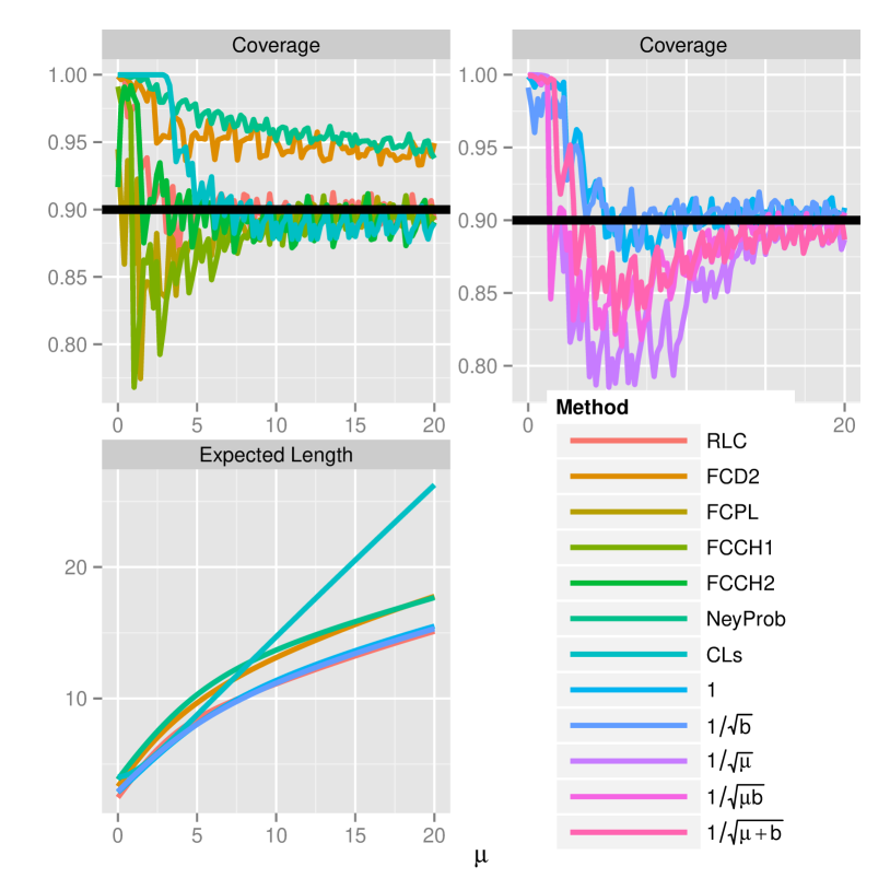
Figure 14: Coverage and Expected Lengths for for the case $b=0.5$, $\tau=1$ and $90\%$ confidence intervals

Let’s begin with a graph of the coverage for the case $b=0.5$, $\tau=1$ and $90\%$ confidence intervals, shown in figure 14. We see surprisingly bad performances of $FCCH1$ and $FCPL$. In the case of $FCCH1$ the minimum occurs for $\mu=1.0$ where the actual coverage is only $77\%$. This turns out to be due to the fact that for the case $x=0$, $y=0$ the upper limit of the 95% interval of $FCCH1$ is only $1.45$, so if we check coverage for (say) $\mu+b=1.5$ this case is excluded, although $f(0,0;1.0,0.5)=0.12$, clearly the probability missing for good coverage.

Similarly the (to) small limit of $FCPL$ for $x=0,y=0$ leads to bad undercoverage, this time at $\mu=1.4$. The coverage of the Bayesian methods with Jeffrey’s prior on $\mu$ is also quite bad, mainly because these priors favor smaller values of $\mu$. Finally the prior $\pi(\mu,b)=1/\sqrt{\mu+b}$ leads to a method with coverage that is somewhat borderline.

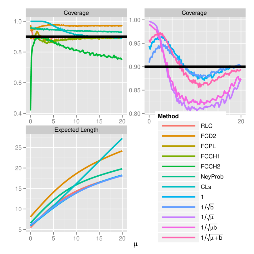
Figure 16: Coverage and Expected Lengths for for the case $b=5$, $\tau=1$ and $90\%$ confidence intervals

Figure 16 shows the coverage for the case $b=5.0$, $\tau=1$ and $90\%$ confidence intervals. Here the worst method is $FCCH2$, with a true coverage of $42\%$ if $\mu=0.0$! This is due to the fact that the averaging over the lower limits leads very quickly to a positive lower limit, for example if $x=2,y=0,\tau=1$ we get the $90\%$ interval $(0.09,4.29)$, and so for $\mu<0.9$ this case is rejected.

Finally we will find the worst coverage of each method by searching over a grid on $0.5\leq b\leq 10$ and $0\leq\mu\leq 20$. The results are shown in table 5. As we saw before $FCCH1$, $FCCH2$, $FCPL$, $1/\sqrt{\mu}$, $1/\sqrt{\mu b}$ and $1/\sqrt{\mu+b}$ show some considerable undercoverage. These methods will therefore be removed from further consideration.

Of course one should repeat the above studies for other values of $\tau$ and other confidence levels. In the appendix we have the corresponding graphs and tables for the cases $\tau=0.5,2$ and $68\%$ and $95\%$ intervals. The results are very similar to those shown here.

3.2 Other Considerations

This leaves us with a choice of six methods. How do we decide among those? Here the experimenter is free to use any criterion he wishes, provided that the choice is made without consideration of the data. We already mentioned two, namely avoiding the problem of flip-flopping and/or avoiding empty intervals. All (except $CLs$, which always yields upper limits) of the methods discussed here have a smooth transition from upper limits to two-sided intervals, and so flip-flopping is not an issue. The only method which could yield empty intervals is $NeyProb$, which might be eliminated from consideration for that reason.

A very common criterion for the performance of confidence intervals in Statistics is the expected mean length, defined by

$$EL(\mu,b)=\sum_{x=0}^{\infty}\sum_{y=0}^{\infty}\left[U(x,y)-L(x,y)\right]f(x,y;\mu,b)$$ (24)

Why short intervals are desirable is most easily seen in the case of upper limits, where it simply means a tighter bound on the parameter of interest. Even in the case of a two-sided interval, knowing that the parameter is most likely in the interval (say) $(2.5,4.9)$ is better than just knowing it is in the interval $(2.1,5.3)$. In general, for confidence intervals the expected length plays a role similar to the concept of power in the case of hypothesis testing.

It should be noted that the expected length is metric dependent. So a change in the parametrization of the problem might also change which method yields shortest expected length.

In figure 14 we show the expected length as a function of $\mu$ for the case $b=0.5$, $\tau=1$ and $90\%$ confidence intervals, and in figure 16 the same for the case $b=5.0$. In both cases $RLC$ has the shortest intervals for small $\mu$ and the Bayesian methods for larger ones. As one would expect the overcoverage observed for $CLs$, $NeyProb$ and $FC2D$ leads to larger expected intervals

4 Conclusions

We have studied the coverage and the expected length of the confidence intervals generated by a number of methods for the “On-Off ” problem. The intervals were derived using a variety of methodologies and include all those in common use today. We find that the $RLC$ limits based on the profile likelihood and the limits derived using the Bayesian methodology with a flat prior on the signal rate $\mu$ are best, all having acceptable coverage and shortest expected length. It is noteworthy that the oldest method in this study, namely the method implemented in MINUIT/MINOS, is still a strong contender even today, at least when used with some adjustments for the cases when $x<y/\tau$ as is done in $RLC$. It should also be mentioned that just because a flat prior on $\mu$ leads to methods with good coverage for the “On-Off ” problem studied here, this does not necessarily mean that flat priors will always be the best choice.

This study was possible because for this simple model we were able to find explicit formulas for the limits. It would obviously be desirable to do similar studies for more complicated models, for example including uncertainties in $\tau$, including efficiencies with their uncertainties as well extensions such as multiple channels. In those cases, though, deriving explicit formulas will be difficult if not impossible, and as soon as MC methods are needed to calculate limits the scope of any coverage study will be severely limited. Nevertheless we hope this study will provide some guidance as to which methods are most promising.

5 Appendix

5.1 Confidence region for Feldman-Cousins

5.2 Graphs and Tables of Coverage and Expected Lengths

5.2.1 Case $\tau=0.5$ and $68\%$ Confidence Intervals

Table 1: Worst coverage of each method, for $0.5\leq b\leq 10$ and $0\leq\mu\leq 20$. $\tau=$ 0.5 $and$ 68 $\%$ confidence intervals

	RLC	FCD2	FCPL	FCCH1	FCCH2	NeyProb	CLs
b	$3$	$0.5$	$0.5$	$0.5$	$10$	$10$	$0.5$
$\mu$	$8.6$	$8.2$	$1.2$	$0.8$	$20$	$19.6$	$6.5$
Coverage	$63.7$	$86.2$	$81.3$	$72.2$	$24.3$	$81.6$	$51.8$

	$1$	$1/\sqrt{\mu}$	$1/\sqrt{b}$	$1/\sqrt{\mu b}$	$1/\sqrt{\mu+b}$
b	$0.5$	$10$	$0.5$	$0.5$	$0.5$
$\mu$	$4.1$	$9$	$4.5$	$0$	$3.3$
Coverage	$59$	$61.9$	$33.5$	$39.3$	$50.2$

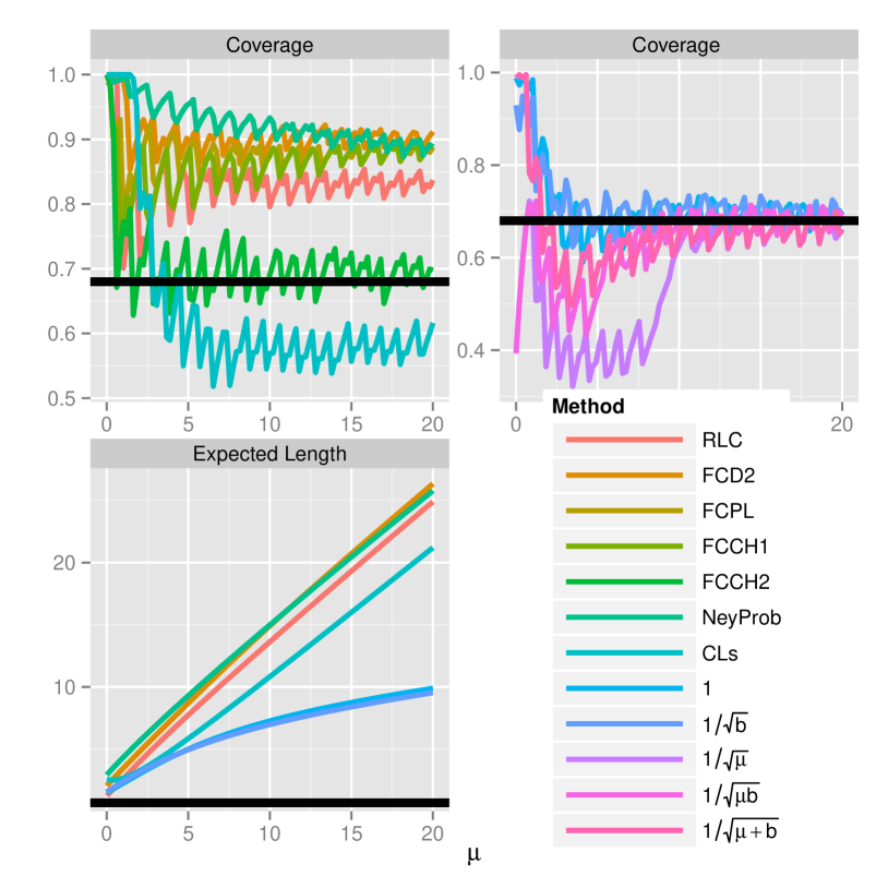
Figure 2: Coverage and Expected Lengths for for the case $b=0.5$, $\tau=0.5$ and $68\%$ confidence intervals

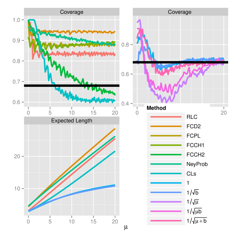
Figure 3: Coverage and Expected Lengths for for the case $b=3$, $\tau=0.5$ and $68\%$ confidence intervals

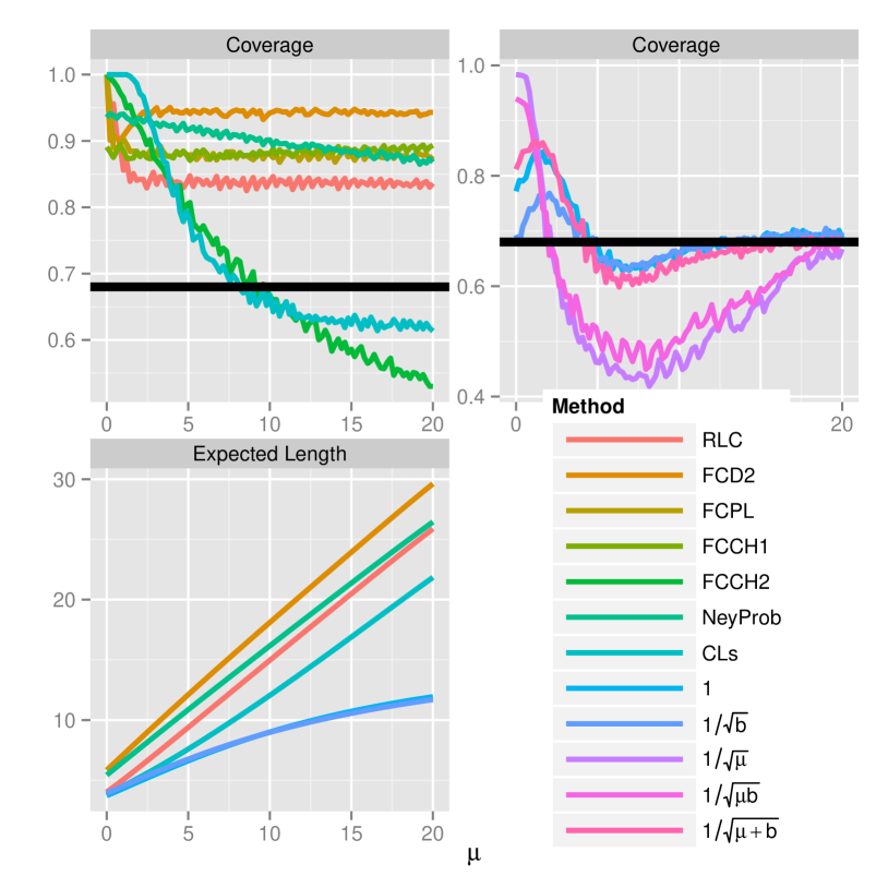
Figure 4: Coverage and Expected Lengths for for the case $b=5$, $\tau=0.5$ and $68\%$ confidence intervals

5.2.2 Case $\tau=0.5$ and $90\%$ Confidence Intervals

Table 2: Worst coverage of each method, for $0.5\leq b\leq 10$ and $0\leq\mu\leq 20$. $\tau=$ 0.5 $and$ 90 $\%$ confidence intervals

	RLC	FCD2	FCPL	FCCH1	FCCH2	NeyProb	CLs
b	$10$	$10$	$3.2$	$0.5$	$10$	$10$	$0.5$
$\mu$	$20$	$0.4$	$0.4$	$1.6$	$0$	$20$	$16.3$
Coverage	$87.8$	$91.8$	$87.8$	$87.4$	$21.1$	$90.3$	$83.8$

	$1$	$1/\sqrt{\mu}$	$1/\sqrt{b}$	$1/\sqrt{\mu b}$	$1/\sqrt{\mu+b}$
b	$0.5$	$10$	$0.5$	$0.5$	$0.5$
$\mu$	$8.2$	$18.8$	$9.4$	$6.5$	$7.8$
Coverage	$83.3$	$86.1$	$73.8$	$78.7$	$79.8$

Figure 5: Coverage and Expected Lengths for for the case $b=0.5$, $\tau=0.5$ and $90\%$ confidence intervals

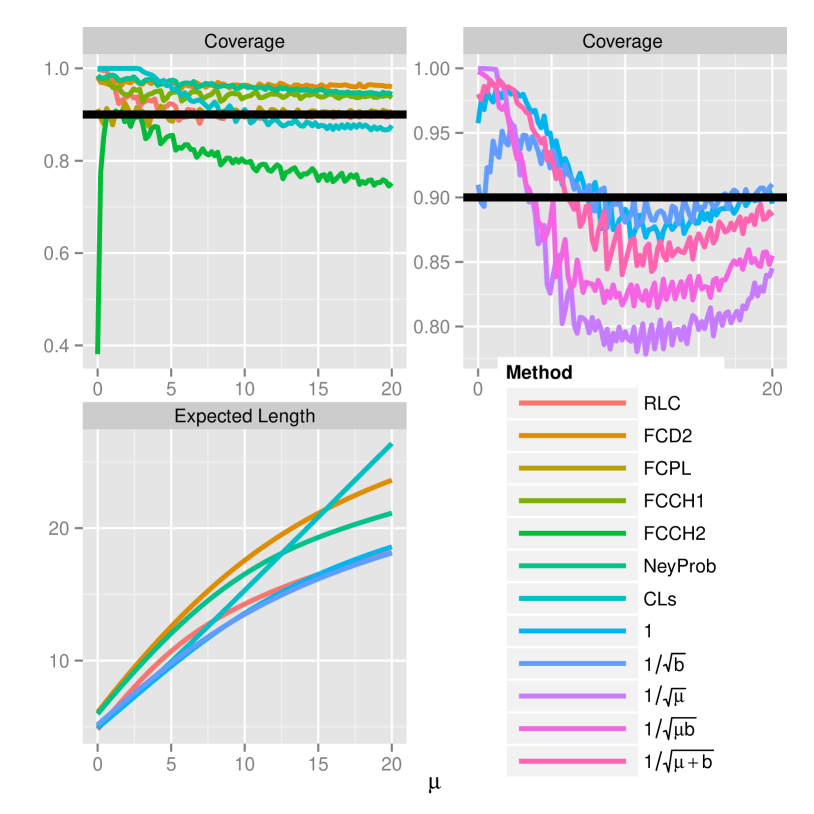
Figure 6: Coverage and Expected Lengths for for the case $b=3$, $\tau=0.5$ and $90\%$ confidence intervals

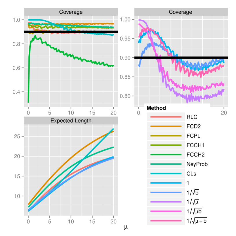
Figure 7: Coverage and Expected Lengths for for the case $b=5$, $\tau=0.5$ and $90\%$ confidence intervals

5.2.3 Case $\tau=0.5$ and $95\%$ Confidence Intervals

Table 3: Worst coverage of each method, for $0.5\leq b\leq 10$ and $0\leq\mu\leq 20$. $\tau=$ 0.5 $and$ 95 $\%$ confidence intervals

	RLC	FCD2	FCPL	FCCH1	FCCH2	NeyProb	CLs
b	$10$	$9.8$	$10$	$10$	$10$	$10$	$0.5$
$\mu$	$20$	$0.4$	$20$	$20$	$0$	$20$	$11.8$
Coverage	$92.6$	$94.8$	$92.6$	$93.6$	$25.6$	$93.6$	$90.9$

	$1$	$1/\sqrt{\mu}$	$1/\sqrt{b}$	$1/\sqrt{\mu b}$	$1/\sqrt{\mu+b}$
b	$10$	$10$	$0.5$	$10$	$0.5$
$\mu$	$20$	$20$	$6.9$	$19.6$	$11.4$
Coverage	$90.9$	$91.6$	$83.8$	$88.2$	$88.8$

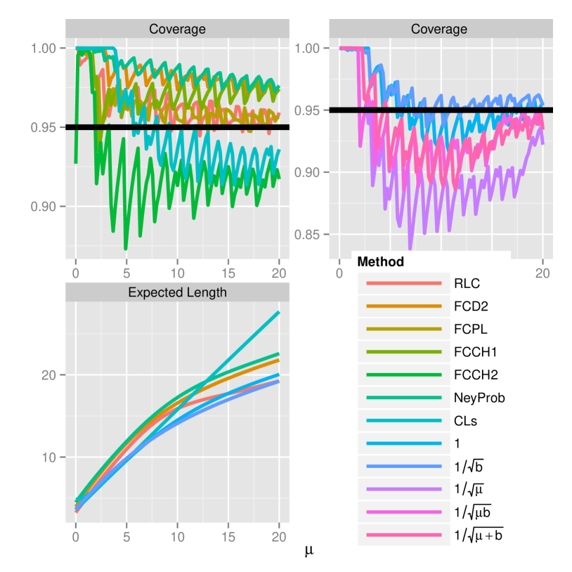
Figure 8: Coverage and Expected Lengths for for the case $b=0.5$, $\tau=0.5$ and $95\%$ confidence intervals

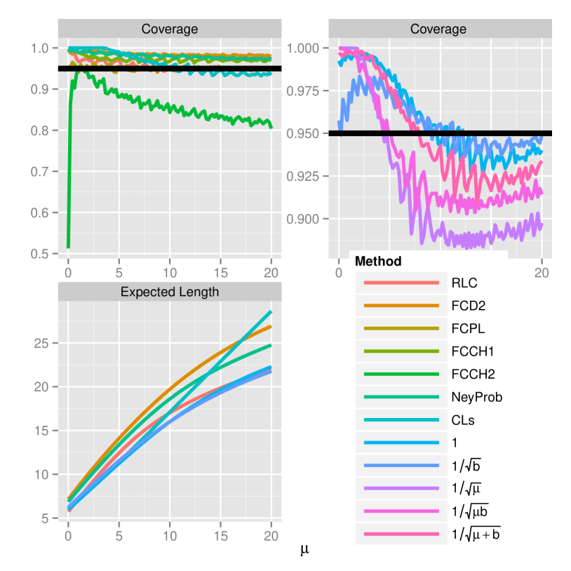
Figure 9: Coverage and Expected Lengths for for the case $b=3$, $\tau=0.5$ and $95\%$ confidence intervals

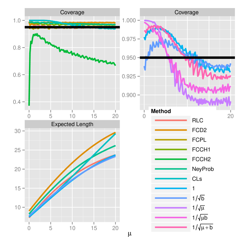
Figure 10: Coverage and Expected Lengths for for the case $b=5$, $\tau=0.5$ and $95\%$ confidence intervals

5.2.4 Case $\tau=1$ and $68\%$ Confidence Intervals

Table 4: Worst coverage of each method, for $0.5\leq b\leq 10$ and $0\leq\mu\leq 20$. $\tau=$ 1 $and$ 68 $\%$ confidence intervals

	RLC	FCD2	FCPL	FCCH1	FCCH2	NeyProb	CLs
b	$1.3$	$0.5$	$0.5$	$0.5$	$10$	$10$	$0.5$
$\mu$	$1.6$	$4.5$	$0.8$	$0.4$	$0$	$20$	$7.3$
Coverage	$63.6$	$79$	$48.3$	$43.1$	$18$	$72.8$	$60.9$

	$1$	$1/\sqrt{\mu}$	$1/\sqrt{b}$	$1/\sqrt{\mu b}$	$1/\sqrt{\mu+b}$
b	$10$	$8.6$	$0.5$	$0.5$	$0.5$
$\mu$	$7.8$	$6.9$	$0$	$2.9$	$2.4$
Coverage	$60.9$	$61.8$	$39.3$	$37.5$	$51.1$

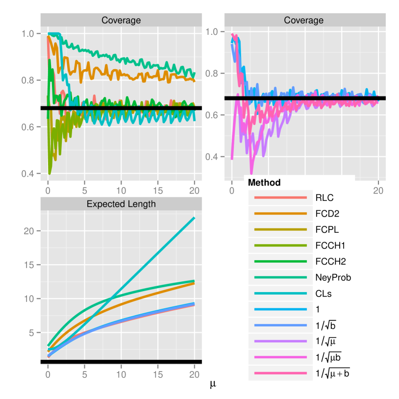
Figure 11: Coverage and Expected Lengths for for the case $b=0.5$, $\tau=1$ and $68\%$ confidence intervals

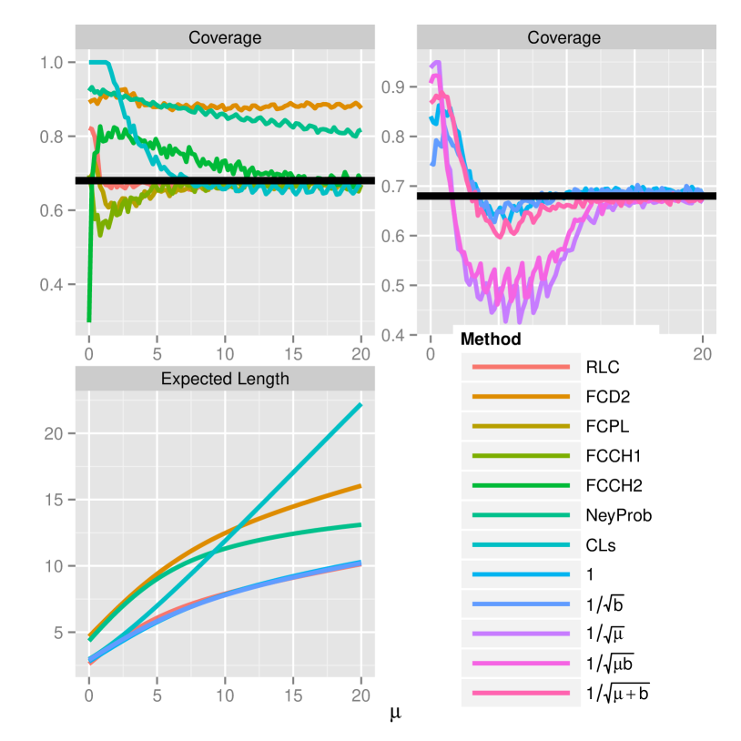
Figure 12: Coverage and Expected Lengths for for the case $b=3$, $\tau=1$ and $68\%$ confidence intervals

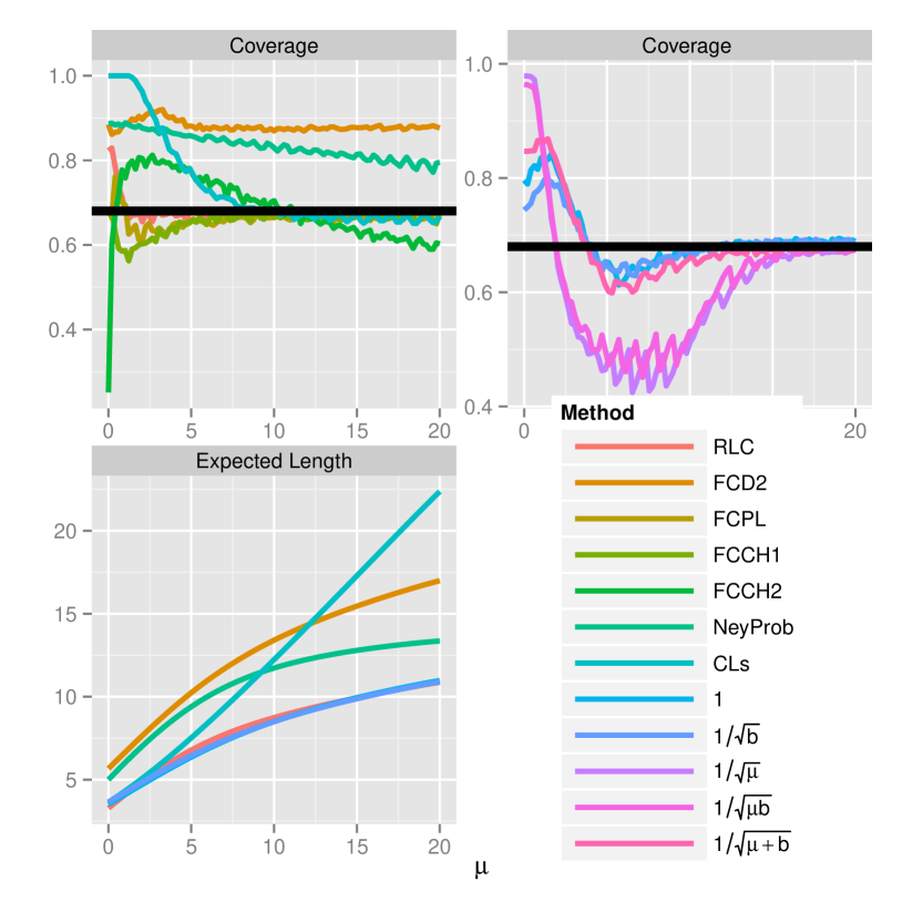
Figure 13: Coverage and Expected Lengths for for the case $b=5$, $\tau=1$ and $68\%$ confidence intervals

5.2.5 Case $\tau=1$ and $90\%$ Confidence Intervals

Table 5: Worst coverage of each method, for $0.5\leq b\leq 10$ and $0\leq\mu\leq 20$. $\tau=$ 1 $and$ 90 $\%$ confidence intervals

	RLC	FCD2	FCPL	FCCH1	FCCH2	NeyProb	CLs
b	$0.5$	$10$	$0.7$	$0.5$	$10$	$10$	$10$
$\mu$	$3.7$	$0.4$	$2.9$	$1.2$	$20$	$20$	$20$
Coverage	$87.7$	$88$	$83.4$	$80$	$28.8$	$90.5$	$86.8$

	$1$	$1/\sqrt{\mu}$	$1/\sqrt{b}$	$1/\sqrt{\mu b}$	$1/\sqrt{\mu+b}$
b	$2.1$	$10$	$0.5$	$10$	$0.5$
$\mu$	$9.8$	$14.7$	$6.9$	$20$	$6.9$
Coverage	$86.9$	$87.4$	$80.4$	$81.3$	$83.9$

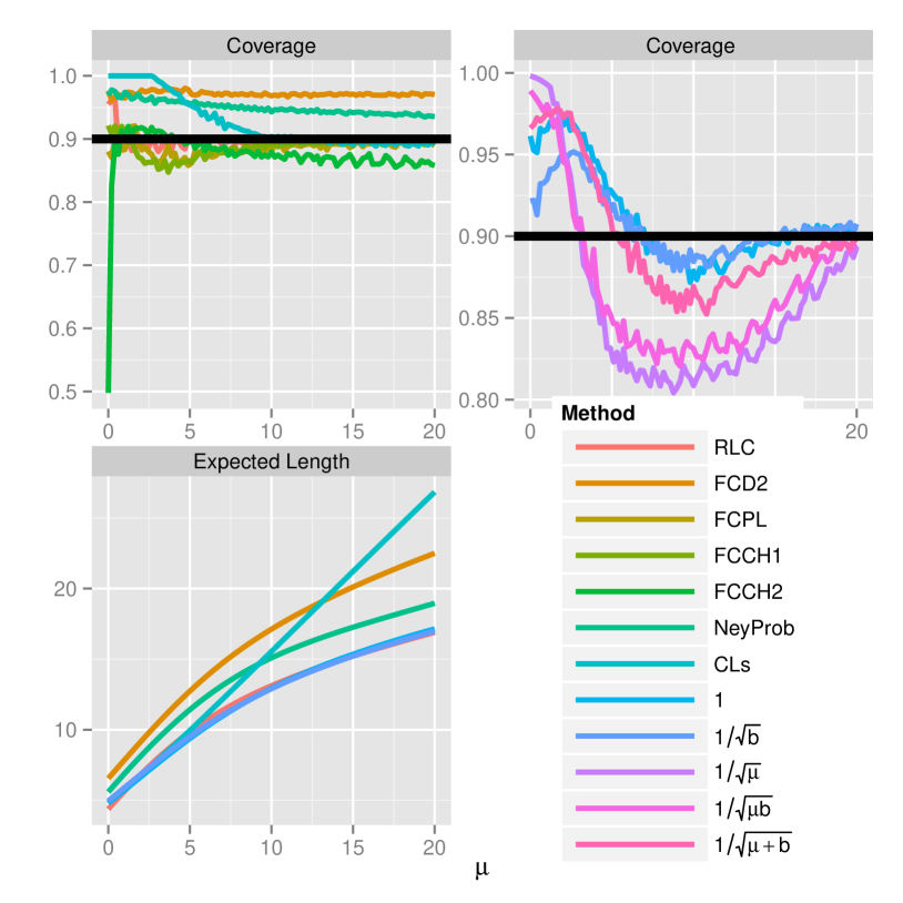
Figure 15: Coverage and Expected Lengths for for the case $b=3$, $\tau=1$ and $90\%$ confidence intervals

5.2.6 Case $\tau=1$ and $95\%$ Confidence Intervals

Table 6: Worst coverage of each method, for $0.5\leq b\leq 10$ and $0\leq\mu\leq 20$. $\tau=$ 1 $and$ 95 $\%$ confidence intervals

	RLC	FCD2	FCPL	FCCH1	FCCH2	NeyProb	CLs
b	$10$	$10$	$0.5$	$0.5$	$10$	$10$	$10$
$\mu$	$20$	$20$	$2$	$1.6$	$19.6$	$20$	$20$
Coverage	$93.1$	$95.9$	$89.4$	$86.8$	$32.5$	$93.9$	$91.8$

	$1$	$1/\sqrt{\mu}$	$1/\sqrt{b}$	$1/\sqrt{\mu b}$	$1/\sqrt{\mu+b}$
b	$10$	$10$	$10$	$10$	$10$
$\mu$	$20$	$20$	$20$	$20$	$20$
Coverage	$91.3$	$91.9$	$87.9$	$89$	$90.7$

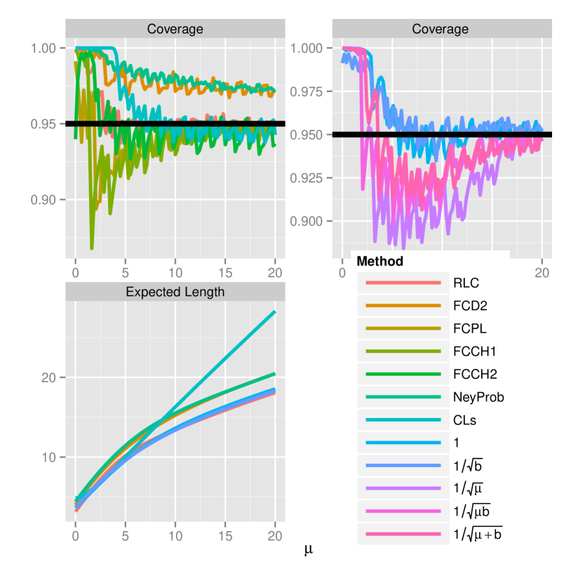
Figure 17: Coverage and Expected Lengths for for the case $b=0.5$, $\tau=1$ and $95\%$ confidence intervals

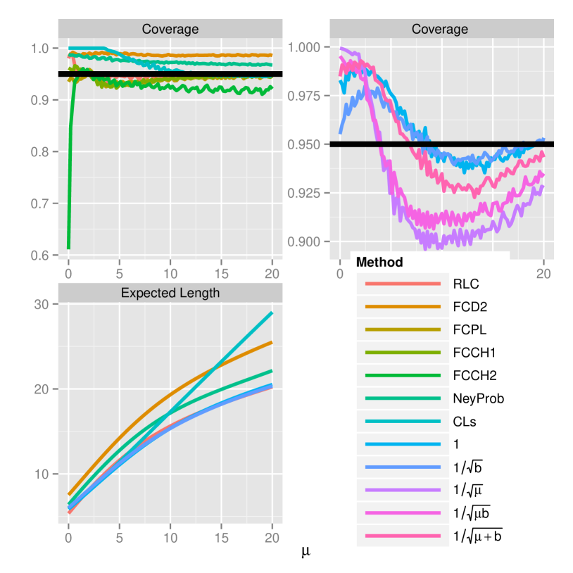
Figure 18: Coverage and Expected Lengths for for the case $b=3$, $\tau=1$ and $95\%$ confidence intervals

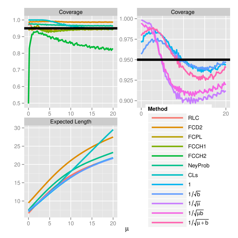
Figure 19: Coverage and Expected Lengths for for the case $b=5$, $\tau=1$ and $95\%$ confidence intervals

5.2.7 Case $\tau=2$ and $68\%$ Confidence Intervals

Table 7: Worst coverage of each method, for $0.5\leq b\leq 10$ and $0\leq\mu\leq 20$. $\tau=$ 2 $and$ 68 $\%$ confidence intervals

	RLC	FCD2	FCPL	FCCH1	FCCH2	NeyProb	CLs
b	$0.5$	$10$	$0.5$	$0.5$	$10$	$10$	$10$
$\mu$	$2.4$	$0$	$0.8$	$0.4$	$20$	$20$	$20$
Coverage	$62.8$	$76.3$	$52.8$	$47$	$23.9$	$67.3$	$65.5$

	$1$	$1/\sqrt{\mu}$	$1/\sqrt{b}$	$1/\sqrt{\mu b}$	$1/\sqrt{\mu+b}$
b	$7.9$	$9.4$	$0.5$	$0.5$	$0.5$
$\mu$	$6.1$	$6.5$	$0$	$0$	$2.9$
Coverage	$61.9$	$62.2$	$38.8$	$38.7$	$56.3$

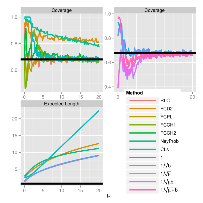
Figure 20: Coverage and Expected Lengths for for the case $b=0.5$, $\tau=2$ and $68\%$ confidence intervals

Figure 21: Coverage and Expected Lengths for for the case $b=3$, $\tau=2$ and $68\%$ confidence intervals

Figure 22: Coverage and Expected Lengths for for the case $b=5$, $\tau=2$ and $68\%$ confidence intervals

5.2.8 Case $\tau=2$ and $90\%$ Confidence Intervals

Table 8: Worst coverage of each method, for $0.5\leq b\leq 10$ and $0\leq\mu\leq 20$. $\tau=$ 2 $and$ 90 $\%$ confidence intervals

	RLC	FCD2	FCPL	FCCH1	FCCH2	NeyProb	CLs
b	$0.5$	$0.5$	$0.5$	$0.5$	$10$	$10$	$10$
$\mu$	$2$	$19.6$	$1.6$	$0.4$	$20$	$20$	$20$
Coverage	$85.6$	$93.6$	$84.8$	$56.8$	$30.4$	$88.1$	$87.3$

	$1$	$1/\sqrt{\mu}$	$1/\sqrt{b}$	$1/\sqrt{\mu b}$	$1/\sqrt{\mu+b}$
b	$10$	$7.7$	$1.9$	$9.4$	$0.5$
$\mu$	$13.5$	$12.2$	$7.8$	$11.8$	$5.3$
Coverage	$87.4$	$87.6$	$79.7$	$82.2$	$84.6$

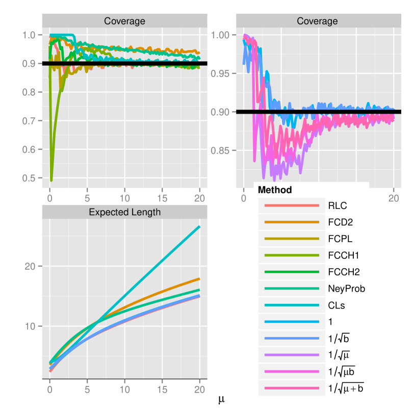
Figure 23: Coverage and Expected Lengths for for the case $b=0.5$, $\tau=2$ and $90\%$ confidence intervals

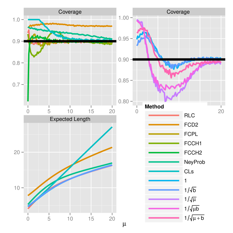
Figure 24: Coverage and Expected Lengths for for the case $b=3$, $\tau=2$ and $90\%$ confidence intervals

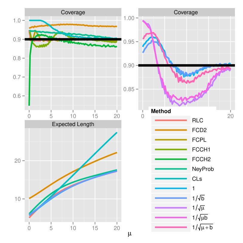
Figure 25: Coverage and Expected Lengths for for the case $b=5$, $\tau=2$ and $90\%$ confidence intervals

5.2.9 Case $\tau=2$ and $95\%$ Confidence Intervals

Table 9: Worst coverage of each method, for $0.5\leq b\leq 10$ and $0\leq\mu\leq 20$. $\tau=$ 2 $and$ 95 $\%$ confidence intervals

	RLC	FCD2	FCPL	FCCH1	FCCH2	NeyProb	CLs
b	$0.5$	$10$	$0.5$	$0.5$	$10$	$10$	$10$
$\mu$	$2.9$	$20$	$2.4$	$0.8$	$20$	$20$	$20$
Coverage	$93.3$	$96.5$	$91.4$	$72.7$	$33.8$	$92.7$	$92.3$

	$1$	$1/\sqrt{\mu}$	$1/\sqrt{b}$	$1/\sqrt{\mu b}$	$1/\sqrt{\mu+b}$
b	$10$	$10$	$10$	$1.1$	$10$
$\mu$	$20$	$20$	$20$	$9.4$	$20$
Coverage	$92.5$	$92.7$	$89.4$	$89.6$	$91.8$

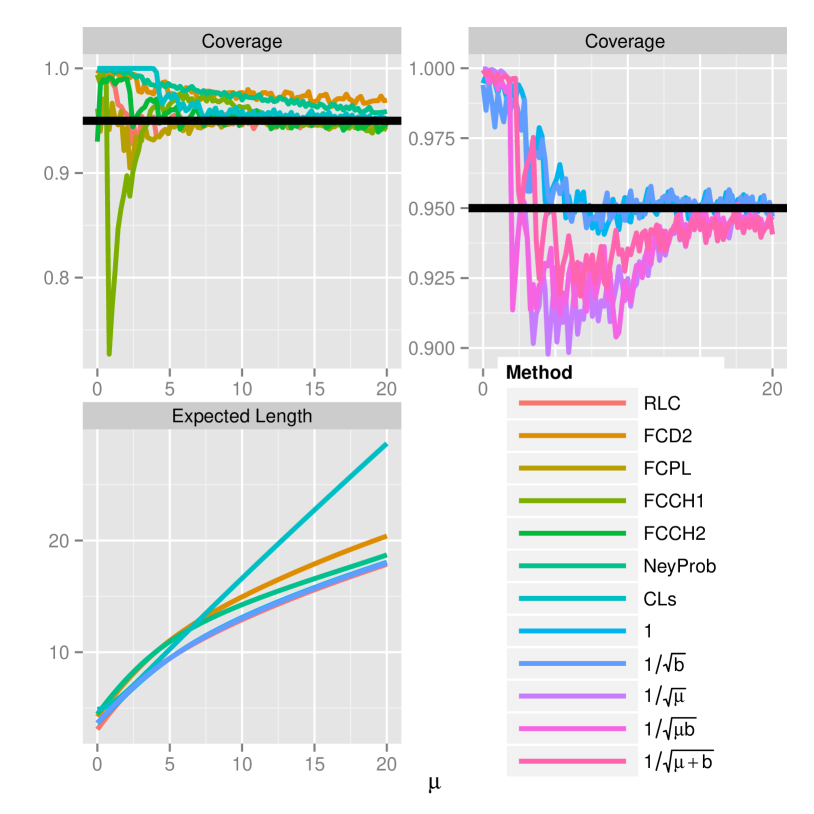
Figure 26: Coverage and Expected Lengths for for the case $b=0.5$, $\tau=2$ and $95\%$ confidence intervals

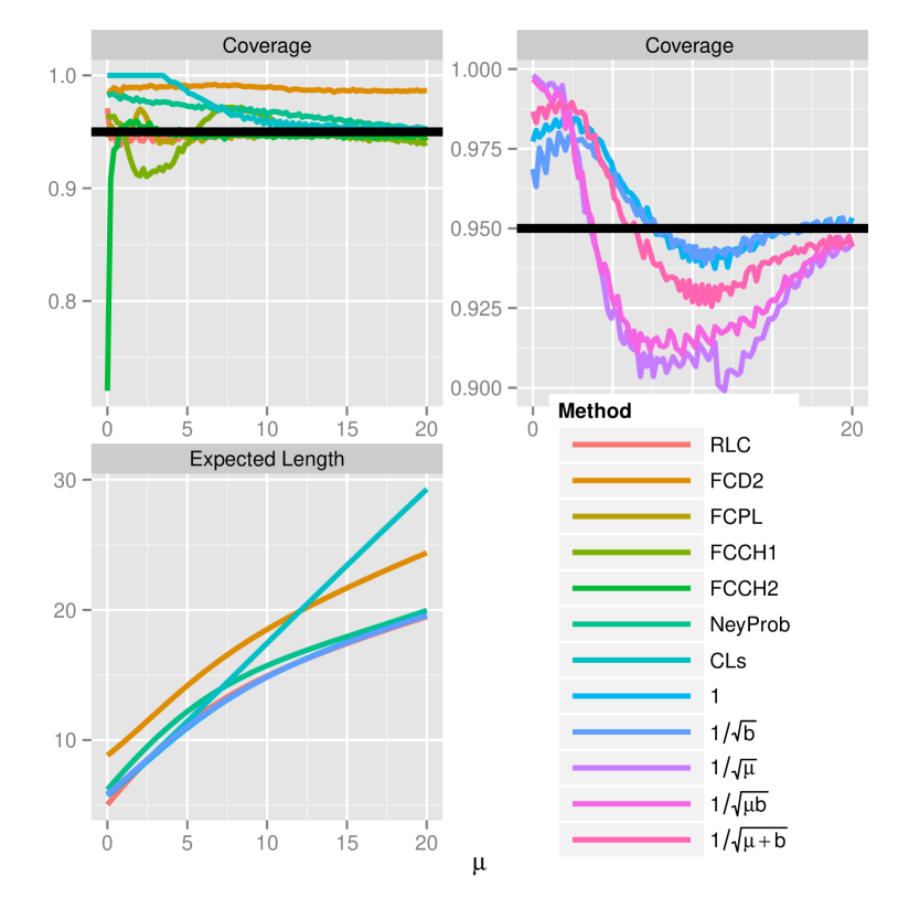
Figure 27: Coverage and Expected Lengths for for the case $b=3$, $\tau=2$ and $95\%$ confidence intervals

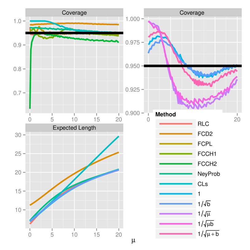
Figure 28: Coverage and Expected Lengths for for the case $b=5$, $\tau=2$ and $95\%$ confidence intervals

References

- [1] Sivan Aldor-Noiman, Lawrence D. Brown, Andreas Buja, Wolfgang Rolke, and Robert A. Stine. The power to see: A new graphical test of normality. Journal of the American Statistican, 67(4):249–260, 2013.
- [2] Andreas Buja and Wolfgang Rolke. Calibration for simultaneity: (re)sampling methods for simultaneous inference with applications to function estimation and functional data, 2003. Technical Report, Department of Statistics, University of Pennsylvania.
- [3] G. Casella and R.L. Berger. Statistical Inference. Duxbury advanced series in statistics and decision sciences. Thomson Learning, 2002.
- [4] Jan Conrad, O. Botner, A. Hallgren, and Carlos Perez de los Heros. Including systematic uncertainties in confidence interval construction for Poisson statistics. Phys.Rev., D67:012002, 2003.
- [5] Robert D. Cousins and Virgil L. Highland. Incorporating systematic uncertainties into an upper limit. Nucl. Instrum. Methods, 1991.
- [6] Robert D. Cousins, James T. Linnemann, and Jordan Tucker. Evaluation of three methods for calculating statistical significance when incorporating a systematic uncertainty into a test of the background-only hypothesis for a Poisson process. Nucl.Instrum.Meth., A595:480–501, 2008.
- [7] Glen Cowan, Kyle Cranmer, Eilam Gross, and Ofer Vitells. Asymptotic formulae for likelihood-based tests of new physics. Eur.Phys.J., C71:1554, 2011.
- [8] Gary J. Feldman and Robert D. Cousins. A Unified approach to the classical statistical analysis of small signals. Phys.Rev., D57:3873–3889, 1998.
- [9] K.K. Gan, J. Lee, and R. Kass. Incorporation of the statistical uncertainty in the background estimate into the upper limit on the signal. Nucl.Instrum.Meth., A412:475–482, 1998.
- [10] O. Helene. Upper Limit of Peak Area. Nucl. Instrum. Meth., 212:319, 1983.
- [11] F. James and M. Roos. Minuit: A System for Function Minimization and Analysis of the Parameter Errors and Correlations. Comput. Phys. Commun., 10:343–367, 1975.
- [12] T. P. Li and Y. Q. Ma. Analysis methods for results in gamma-ray astronomy. Astrophys. J., 272:317–324, 1983.
- [13] J. Lundberg, J. Conrad, W. Rolke, and A. Lopez. Limits, discovery and cut optimization for a Poisson process with uncertainty in background and signal efficiency: TRolke 2.0. Comput. Phys. Commun., 181:683–686, 2010.
- [14] Alexander L. Read. Presentation of search results: The CL(s) technique. J.Phys., G28:2693–2704, 2002.
- [15] Wolfgang A. Rolke and Angel M. Lopez. Confidence intervals and upper bounds for small signals in the presence of background noise. Nucl.Instrum.Meth., A458:745–758, 2001.
- [16] Wolfgang A. Rolke, Angel M. Lopez, and Jan Conrad. Limits and confidence intervals in the presence of nuisance parameters. Nucl.Instrum.Meth., A551:493–503, 2005.
- [17] Fredrik Tegenfeldt and Jan Conrad. On Bayesian treatement of systematic uncertainties in confidence interval calculations. Nucl.Instrum.Meth., A539:407–413, 2005.
- [18] Gunter Zech. Upper Limits in Experiments with Background Or Measurement Errors. Nucl.Instrum.Meth., A277:608, 1989.