Quark matter under strong magnetic fields

Abstract

We revisit three of the mathematical formalisms used to describe magnetized quark matter in compact objects within the MIT and the Nambu-Jona-Lasinio models and then compare their results. The tree formalisms are based on 1) isotropic equations of state, 2) anisotropic equations of state with different parallel and perpendicular pressures and 3) the assumption of a chaotic field approximation that results in a truly isotropic equation of state. We have seen that the magnetization obtained with both models is very different: while the MIT model produces well-behaved curves that are always positive for large magnetic fields, the NJL model yields a magnetization with lots of spikes and negative values. This fact has strong consequences on the results based on the existence of anisotropic equations of state. We have also seen that, while the isotropic formalism results in maximum stellar masses that increase considerably when the magnetic fields increase, maximum masses obtained with the chaotic field approximation never vary more than 5.5$\%$. The effect of the magnetic field on the radii is opposed in the MIT and NJL models: with both formalisms, isotropic and chaotic field approximation, for a fixed mass, the radii increase with the increase of the magnetic field in the MIT bag model and decrease in the NJL, the radii of quark stars described by the NJL model being smaller than the ones described by the MIT model.

1 Introduction

The influence of magnetic fields ($B$) in the formation, constitution and evolution of stars is a topic of intense investigation and discussion. Some astronomers believe that magnetism plays an essential role in the star formation, second only to gravitation zirker . As the star burns its fuel, depending on its mass, it may end as a white dwarf or a neutron star and in both cases, magnetic fields can be quite intense. Neutron stars are very dense compact objects with magnetic fields generally of the order of $10^{12}$ G and they are mainly detected as pulsars, powered by rotation energy, or as accreting X-ray binaries, powered by gravitational energy. However, since 1979, other classes of neutron stars have been observed as either soft gamma-ray repeaters or as anomalous X-ray pulsars with no binary companion. These objects bear magnetic fields of the order of $10^{14}-10^{16}$ G and were named magnetars magnetars .

If one observes the QCD phase diagram, neutron stars lie in a region of low temperatures and high baryonic chemical potentials $\mu$ (or baryonic densities, if one prefers). If these objects are affected by the presence of strong magnetic fields, other regions of the QCD phase diagram should be affected as well qcd+b ,CEP1 .

The region of high temperatures and low chemical potentials is the relevant regime for the study of heavy ion collisions kharzeev and in these experiments, the field intensity probably decreases very rapidly, lasting for about 1-2 fm/c only, but a possible signature of the strong magnetic fields has been investigated tuchin ,mclerran , event , paoli , photon_anisotropy . Moreover, this region of high-$T$/low-$\mu$, has already been exploited using Lattice (LQCD) simulations. The QCD phase diagram presents a first order transition at low-$T$/high-$\mu$ region and a crossover region at high-$T$/low-$\mu$ and these two regions may be connected by a critical end point CEP1 ,CEP2 . LQCD results point out, in accordance with most model predictions, that the crossover observed at $B=0$ does not disappear when $B\neq 0$ earlylattice ,preussker ,lattice1 ,lattice2 . Nevertheless the region of low-$T$/high-$\mu$ remains unavailable to LQCD assessments and hence, the physical properties related to this region can only be investigated with the help of (effective) models.

Other important aspects related to magnetized quark matter are the richness of its internal substructures and the inverse magnetic catalysis (IMC). Although the results are model dependent, the internal structure of the QCD phase diagram has been shown to be very rich structure , presenting lots of intermediate phases, due to the small jumps in the quark dressed masses, which are related to the filling of the Landau levels. Concerning the IMC, LQCD calculations predict an inverse catalysis, with the pseudo-critical temperature decreasing with $B$ lattice1 ; lattice2 , while most effective models predict an increase of the pseudo-critical temperature with $B$ catalysis-ours , ricardo . It is a common belief that this deficiency in effective models is due to the fact that they do not account for back reaction effects (the indirect interaction of gluons with the magnetic field) teoriaIMC .

One important point that should not be disregarded refers to the contribution of the electromagnetic interaction to the pressure(s) and energy density, a term proportional do $B^{2}$, where $B$ is the magnetic field strength. Astrophysicists advocate that the magnetic field in the surface of magnetars is of the order of $10^{15}$G. However, according to the Virial theorem one could expect fields three or four orders of magnitude stronger in their interior. To cope with this difference in strength, an ad hoc exponential density-dependent magnetic field was proposed in ref. Pal and adopted in many other works Mao ,Rabhi , prc2 , rudiney , Ryu , Rabhi2 , Mallick , luizlaercio ,Dex ,njlv , Mallick2 ,Ro . Another similar prescription for an energy density dependent magnetic field was proposed in Ref. chaotic . The second prescription seems more natural because the quantity used in the TOV equations tov to calculate the macroscopic quantities is the energy density and not the number density. Moreover, in chaotic , it is shown that this choice reduces the number of free parameters and it is given by:

$$B(\epsilon)=B_{0}\bigg{(}{\frac{\epsilon_{M}}{\epsilon_{0}}}\bigg{)}^{\gamma}+B^{surf},$$ (1)

where $B_{0}$ is the fixed value of the magnetic field, $\epsilon_{0}$ is the energy density at the center of the maximum mass neutron star with zero magnetic field, $\epsilon_{M}$ is the energy density of the matter alone, avoiding a self-generated magnetic field, and $\gamma$ is any positive number. In the present work we take $\gamma=3$ and thus, we reduce the number of free parameters from two, used in the prescription proposed in Pal to only one. Nevertheless, as pointed in ref. chaotic , for chaotic magnetic fields, Eq. (1) yields a parameter-free model, while for the standard density-dependent magnetic field, the macroscopic properties are strongly dependent of these two non-observables parameters. Another point worth mentioning is that the magnetic field is no longer fixed for all neutron star configurations. Each equation of state (EOS) produces a different value for $\epsilon_{0}$ that enters in Eq. (1). In this sense, $\epsilon_{0}$ is also another parameter, but it is not arbitrary as $\gamma$ and the two parameters that can be arbitrarily changed in the parametrization proposed in ref. Pal . It comes directly from the model that defines the EOS, as the baryonic density, pressure and energy density that enter as input to the TOV tov .

One should bear in mind that these two ansätze, violate Maxwell equations because the divergent of $B$ is no longer zero. To minimize this problem, in the present work only the contribution to the term proportional to $B^{2}$ will be taken as density dependent. The EOS obtained from magnetized matter will always carry a fixed $B$ value. With this choice, if we apply the models to describe stellar matter, we guarantee thermodynamical consistency in the EOS and still force matter at the surface of the star to be subject to a magnetic field that is not too strong. It is also important to stress that if a density dependent magnetic field is used through out the calculations, numerical results are almost coincident with the ones we present next but, besides violating Maxwell equations, thermodynamical consistency would also require an extra term, normally disregarded in the literature. This point will be specifically emphasized when the equations are displayed in the next sections.

In the present work we study quark matter possibly present in strange (quark) stars. According to the Bodmer-Witten conjecture Itoh ,bodmer ,witten , the interior of a neutron-like star does not consist primarily of hadrons, but rather of quark matter composed of deconfined up, down and strange quarks, plus the leptons necessary to ensure charge neutrality and $\beta$-equilibrium. When a model is chosen, it is important to verify if it satisfies the necessary conditions that ensure that quark matter is the true ground state: two-flavor quark matter must be unstable (i.e., at zero temperature its energy per baryon has to be larger than 930 MeV, the iron binding energy) and the three-flavor quark matter must be stable (i.e., its energy per baryon must be lower than 930 MeV, also at $T=0$). Not all quark matter models satisfy these conditions and the NJL model only provides absolute stable matter when it is magnetized stabilityB . As already said, according to the Virial theorem and assuming uniform field and mass density, the maximum magnetic field allowed in a gravitationally bound star is smaller than $10^{19}$ G. However, a quark star is self-bound by the nuclear interaction and a simple estimative of the maximum allowed magnetic field gives fields of the order of $10^{20}$ G efrain ; noronha2007 . We use these values as a guide to our study.

It is worth mentioning that calculations that take into account the effects of the anomalous magnetic moments (AMM) of the quarks forsee that the maximum possible magnetic field strength is 8.6 $\times 10^{17}$ G due to the fact that the $u$ quark polarization would become complex for higher values aurora1 . On the other hand, works on hadronic stellar matter show that the influence of the (nucleonic and hyperonic) AMM on the EOS is minor rudiney ,rhabi1 , if the magnetic fields are of the order of $B=10^{18}$ G. However, if $B>10^{18}$G, the inclusion of the anomalous magnetic moment contribution stiffens the stellar matter EOS, and may originate a total spin polarization of neutrons broderick00 . In the present work, we do not consider the coupling between the field and the quark anomalous magnetic moment, but we think this problem should be tackled in a future work. We come back to this point in the conclusions of the paper.

Despite the fact that usually a mean field approximation is necessary when one uses effective models, restricting their scope and the interpretation of their results, they can be very helpful if one wants to understand the physics not assessed by LQCD. Thus, different models have been recently used to describe quark matter subject to magnetic field, the most common ones being the MIT bag model mit and the Nambu-Jona-Lasinio model njl . In the present work we revisit both of them within three different formalisms employed in the literature to describe stellar matter.

The first formalism considers that quark matter is isotropic blandford and it was used in the seminal works on magnetars described either by a quark matter chakra96 or by a hadronic matter equation of state lattimer_2000 and in subsequent calculations rhabi1 ,rhabi2 . The first calculations involving quark matter described by the NJL model followed the same line of understandingprc2 ,rudiney , luizlaercio , prc1 .

The second formalism is based on the fact that the EOS cannot be truly isotropic, once the components of the energy-momentum tensor are not equal, giving different contributions for the parallel and perpendicular pressure efrain , aurora1 , sedrakian , jorge , aurora2 . Moreover, under strong magnetic fields, the $O(3)$ rotational symmetry breaks, and this is another argument that supports the existence of pressure anisotropy. Once the EOS is obtained, one observes at what magnetic field the pressures start to deviate from each other and this is the limit usually taken as input to the Tolman-Oppenheimer-Volkoff equations (TOV) tov . As pointed in ref. sedrakian , this limit is around $3.1\times 10^{18}$G. In practice, the EOS used to compute the stellar macroscopic quantities is isotropic aurora1 , jorge ,veronica . However, this approach means that one recognizes that the system is anisotropic but ends up ignoring this fact. At least two recent works face this problem: in one of them Mallick2 , the authors treated the anisotopic pressures as a perturbation in a way similar to the Hartle-Thorn method, generally used for slowly rotating neutron stars. In the other one aurora2 , an axisymmetric geometry is assumed and the Einstein equations are solved with the adoption of a cylindrical symmetric metric. Older works also tackle this subject Bocquet , Cardall . In the present work we do not intend to reproduce these more sophisticated treatments, but we will investigate the effects of strong magnetic fields on the anisotopic pressures.

Finally, the underlying assumption of the third formalism is that in the presence of anisotropies, the concept of pressure has to be taken with care Misner ; Zel . Based on the concepts discussed in these two books, a small-scale chaotic field is used and the stress tensor is modified accordingly, so that the resulting EOS is a truly isotropic one chaotic .

Next, a comparison of the results obtained with the three formalisms is shown and discussed. Although parts of this material are already available in the literature, a correct comparison can only be made if the same choice for the magnetic field is used. In the present work we use the energy density dependent magnetic field given in Eq. (1) to compute our results with the three formalisms. We would like to emphasize that our aim in the present work is not to justify, criticize or choose any of the formalisms just mentioned. We restrict ourselves to the analysis and comparison of the results.

The present work is organized as follows: in Section 2, we present the EOS obtained for the MIT bag model in the presence of a magnetic field in one preferential direction with the three possible formalisms just discussed: an isotropic EOS, an anisotropic EOS with different parallel and perpendicular pressures and another isotropic EOS resulting from the introduction of a chaotic field. The main results are then shown and discussed. In Section 3, the same steps are taken for the NJL model. In Section 4, some of the results obtained with both models are compared. Finally, in the last Section, the final conclusions are drawn.

2 The MIT Bag model

The EOS for magnetized quark matter described by the MIT bag model has already been extensively studied efrain , aurora1 , sedrakian , jorge , aurora2 . We next show only the Lagrangian density and the resulting EOS. We depart from the following Lagrangian density:

$${\cal L}={\cal L}_{f}+{\cal L}_{l}-\frac{1}{4}F_{\mu\nu}F^{\mu\nu}\,,$$ (2)

which contains a quark sector, ${\cal L}_{f}$, a leptonic sector, ${\cal L}_{l}$, and the electromagnetic contribution $F_{\mu\nu}=\partial_{\mu}A_{\nu}-\partial_{\nu}A_{\mu}$. We use a static and constant magnetic field parallel to the $z$ direction and hence, we choose the gauge $A_{\mu}=\delta_{\mu 2}x_{1}B$ and the energy levels in the $x$ and $y$ directions are quantized.

The leptonic sector is described by

$$\mathcal{L}_{l}=\bar{\psi}_{l}\left[\gamma_{\mu}\left(i\partial^{\mu}-q_{l}A^{\mu}\right)-m_{l}\right]\psi_{l}\,\,,$$ (3)

where $l=e,\mu$. As we restrict ourselves to the $T=0$ case, the star has no more trapped neutrinos, which have escaped and carried a huge amount of energy while the star cooled down.

The thermodynamical potential for the three flavor quark sector, $\Omega_{f}$, can be written as

$$\Omega_{f}=-P_{f}={\cal E}_{f}-\sum_{f}\mu_{f}n_{f},$$ (4)

where $P_{f}$ represents the pressure, ${\cal E}_{f}$ the energy density, $\mu_{f}$ the chemical potential, and $n_{f}$ the quark number density. A similar expression can be written for the leptonic sector.

2.1 MIT - Isotropic EOS

In order to obtain the complete EOS, the pressure, and baryonic density were calculated in stabilityB , efrain , sedrakian and are given by

$$P_{f}=\sum_{k=0}^{k_{f,max}}\alpha_{k}\frac{|q_{f}|BN_{c}}{4\pi^{2}}\left[\mu_{f}\sqrt{\mu_{f}^{2}-s_{f}(k,B)^{2}}\right.$$

$$\left.-s_{f}(k,B)^{2}\ln\left(\frac{\mu_{f}+\sqrt{\mu_{f}^{2}-s_{f}(k,B)^{2}}}{s_{f}(k,B)}\right)\right]-\mathcal{B}\mbox{,}$$ (5)

where $N_{c}$ is the number of colors, $q_{f}$ is the electric charge of each quark, $B$ is the magnetic field strength and the quark masses are $m_{u,d}=5$ MeV, $m_{s}$=120 MeV, $\mathcal{B}$ is the bag constant fixed as 148 MeV^1/4, $\alpha_{0}=1,\,\alpha_{k>0}=2$,

$$s_{f}(k,B)=\sqrt{m_{f}^{2}+2|q_{f}|Bk}$$ (6)

and

$$n=\sum_{i}\frac{n_{f}}{3},$$ (7)

with

$$n_{f}=\sum_{k=0}^{k_{f,max}}\alpha_{k}\frac{|q_{f}|BN_{c}}{2\pi^{2}}k_{F,f}\mbox{,}$$ (8)

where $k_{F,f}=\sqrt{\mu_{f}^{2}-s_{f}(k,B)^{2}}$. At $T=0$, the upper Landau level (or the nearest integer) is defined by

$$k_{f,max}=\frac{\mu_{f}^{2}-m_{f}^{2}}{2|q_{f}|B}=\frac{k_{F,f}^{2}}{2|q_{f}|B},$$ (9)

and the energy density can be easily obtained from Eqs. (4),(5) and (8).

In the description of compact stars, both charge neutrality and chemical equilibrium conditions have to be imposed Glen00 . The first condition can be written for quarks and leptons as

$$2n_{u}=n_{d}+n_{s}+3\left(n_{e}+n_{\mu}\right)\mbox{,}$$ (10)

and the second condition can be written as

$$\mu_{s}=\mu_{d}=\mu_{u}+\mu_{e}\mbox{, \ \ }\mu_{e}=\mu_{\mu}\mbox{,}$$ (11)

where the lepton densities can be calculated through Eq. (8), with appropriate substitutions for the masses and electric charge. The lepton masses are $m_{e}=0.511$ MeV and $m_{\mu}=105.66$ MeV. For the electron and muon pressure ($P_{l}$) and energy density ($\epsilon_{l}$) we use Eqs. (5) and the leptonic analogue of Eq.(4), respectively, all with $\mathcal{B}=0$. In all cases, $N_{c}=1$ for the leptons.

The final expressions for the total pressure and energy density are given by

$$P_{iso}=P_{f}+P_{l}+B(\epsilon)^{2}/2,$$ (12)

$$\epsilon_{iso}=\epsilon_{f}+\epsilon_{l}+B(\epsilon)^{2}/2.$$ (13)

2.2 MIT - Anisotropic EOS

The magnetization of the system is given by

$${\cal M}={dP}/{dB},$$ (14)

and for the quark sector of the MIT bag model, it reads:

$${\cal M}_{f}=\sum_{k=0}^{k_{f,max}}\alpha_{k}\frac{|q_{f}|N_{c}}{4\pi^{2}}\left[\mu_{f}\sqrt{\mu_{f}^{2}-s_{f}(k,B)^{2}}\right.$$

$$\left.-(m_{f}^{2}+4|q_{f}|Bk)\ln\left(\frac{\mu_{f}+\sqrt{\mu_{f}^{2}-s_{f}(k,B)^{2}}}{s_{f}(k,B)}\right)\right]\mbox{.}$$ (15)

In an anisotropic system, the parallel and the perpendicular components of the pressure can be written in terms of the magnetization, as Mallick , efrain , sedrakian , veronica , aurora2 :

$$P_{\parallel}=P_{f}+P_{l}-B(\epsilon)^{2}/2,\quad P_{\perp}=P_{f}+P_{l}-{\cal M}B+B(\epsilon)^{2}/2\mbox{.}$$ (16)

For a magnetic field in the $z$ direction, the stress tensor has the form: diag$(B^{2}/2,B^{2}/2,-B^{2}/2)$ and this explains the difference in sign appearing in the parallel and perpendicular pressures. The energy density is the same as in the isotropic system, given by Eq. (13).

The magnetization for the lepton sector can be read off Eq.(15) with the appropriate substitutions specified below.

2.3 MIT - Chaotic field

According to Misner , as the components of the stress tensor are not equal (they differ in sign), the quantity $\pm B^{2}/2$ cannot be simply added to the pressure terms. As already stated above, for a magnetic field in the $z$ direction, the stress tensor is given by diag$(B^{2}/2,B^{2}/2,-B^{2}/2)$. One way of circumventing this problem is proposed in Zel , where it is shown that, for a small scale chaotic field, the concept of isotropic pressure is recovered because the stress tensor is diag$(B^{2}/6,B^{2}/6,B^{2}/6)$, the $O(3)$ rotational symmetry remains valid and hence, the pressure becomes:

$$P=\frac{1}{3}<T_{i}^{i}>=\frac{1}{3}\bigg{(}\frac{B^{2}}{6}+\frac{B^{2}}{6}+\frac{B^{2}}{6}\bigg{)}=\frac{B^{2}}{6}.$$ (17)

Note that Eq. (17) represents the true thermodynamic pressure, since the components of the stress tensor are equal Zel , in opposition to the two first formalisms. We would like to point out that due to strong heat transportation, the existing turbulence could create a chaotic field. Of course, as the star cools down, the fields could become ordered. The possible mechanisms responsible for creating and maintaining a chaotic field would have to be better investigated and are beyond the scope of the present work.

Within this formalism, the expressions for the total pressure and energy density are given by:

$$P_{chao}=P_{f}+P_{l}+B(\epsilon)^{2}/6,$$ (18)

$$\epsilon_{chao}=\epsilon_{f}+\epsilon_{l}+B(\epsilon)^{2}/2.$$ (19)

2.4 Results MIT

We next show our results for the EOS obtained from the three formalisms just discussed. We have used $\epsilon_{0}=6.93$ fm^-3 in Eq. (1) because this value is the central energy density of the maximum mass obtained with the MIT model for non-magnetized matter with our choice of values for the quark masses and the Bag constant. Before we proceed, it is important to stress that in Eqs. (12), (16) and (18), the magnetic field is taken as constant in $P_{f}$ and $P_{l}$ and Eq.(1) is used in the last terms only. The same holds for the energy density terms.

We first analyze how the magnetization varies with density for different values of the magnetic field in Fig. 1. It is clear that the number of van alphen oscillations are larger for lower values of the magnetic field as expected, due to the larger number of filled Landau levels. As the magnetic field increases, the magnetization of the system also increases and hence, a stronger effect is felt on the anisotropy of the system, as can be seen in Eq. (16).

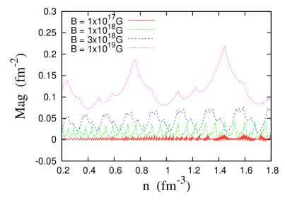
Figure 1: Magnetization as a function of the number density for the MIT bag model.

For $B=10^{17}$ G, the magnetization is negligible and no visible difference can be seen when the perpendicular and parallel pressures are plotted. Moreover, the contribution coming from the term proportional do $B^{2}$ is also too small and, either it is included or not, the plots are coincident. For these reasons, we just plot results for magnetic fields larger than $10^{18}$ G. In Figs. (2) and (5), we plot the parallel and perpendicular pressures for $B=10^{18}$ G respectively without and with the contribution proportional to the $B^{2}$ term. In Figs. (3) and (6), (4) and (7), the same is displayed for a larger magnetic fields, equal to $B=3\times 10^{18}$ G and $B=10^{19}$ G. By analyzing these figures, it is evident that the contribution of the $B^{2}$ term has quite drastic effects on the point where the pressures start to split and hence, as this term is important in stellar matter EOS, it is indeed difficult to justify the use of the TOV equations for magnetic fields larger than $10^{18}$ G. One can also see, from Figs. (5), (6) and (7) that the isotropic pressure does not deviate much from the perpendicular pressure, the only difference being due to the magnetization of the system, which is still relatively small for these fields. The parallel pressure goes to zero at energy densities typical to neutron star core if $B=10^{19}$ G, but for lower magnetic fields, the decrease starts at much higher densities.

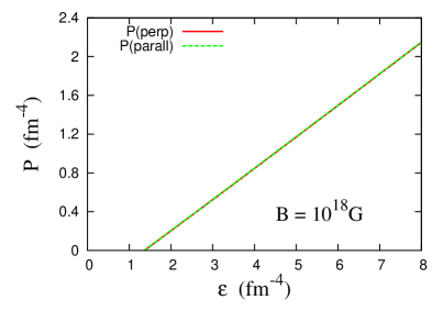
Figure 2: MIT bag model EOS obtained for $B=10^{18}$ G without the term proportional to $B^{2}$

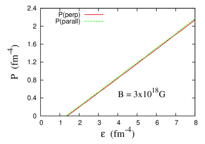
Figure 3: MIT bag model EOS obtained for $B=3\times 10^{18}$ G without the term proportional to $B^{2}$

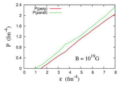
Figure 4: MIT bag model EOS obtained for $B=10^{19}$ G without the term proportional to $B^{2}$

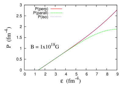
Figure 5: MIT bag model EOS obtained for $B=10^{18}$ G with the term proportional to $B^{2}$

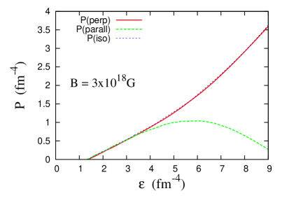
Figure 6: MIT bag model EOS obtained for $B=3\times 10^{18}$ G with the term proportional to $B^{2}$

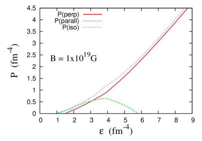
Figure 7: MIT bag model EOS obtained for $B=10^{19}$ G with the term proportional to $B^{2}$

In Fig. (8), the EOS obtained with the assumption of chaotic fields are shown. They deviate very little from non-magnetized matter, with a consequent small variation in the stellar properties that are computed next.

Figure 8: MIT bag model EOS for different values of the chaotic magnetic field.

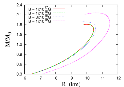
Figure 9: MIT bag model: Mass-radius relation within isotropic pressure for different values of magnetic field.

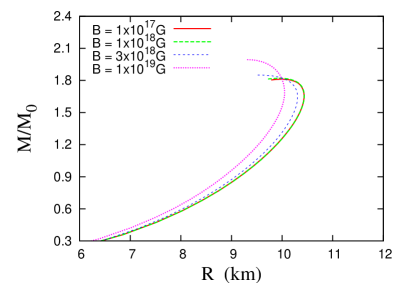
Figure 10: MIT bag model: Mass-radius relation within anisotropic pressure for different values of magnetic field.

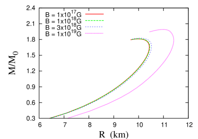
Figure 11: MIT bag model:Mass-radius relation within chaotic magnetic field approximation for different values of magnetic field.

Table 1: Properties of the maximum mass quark star

Model	$B$	$M_{max}$	$Mb_{max}$	R	${\cal E}_{c}$
	(G)	($M_{\odot}$)	($M_{\odot}$)	(km)	(fm-4)
MITisotropic	$10^{17}$	1.81	2.32	9.99	6.77
MITanisotropic	$10^{17}$	1.81	2.32	9.99	6.83
MITchaotic	$10^{17}$	1.81	2.32	9.99	6.80
MITisotropic	$10^{18}$	1.82	2.33	9.97	6.77
MITanisotropic	$10^{18}$	1.82	2.33	9.95	6.85
MITchaotic	$10^{18}$	1.82	2.32	10.03	6.63
MITisotropic	$3.10^{18}$	1.89	2.42	9.78	7.52
MITanisotropic	$3.10^{18}$	1.85	2.36	9.58	7.63
MITchaotic	$3.10^{18}$	1.83	2.33	10.08	6.63
MITisotropic	$10^{19}$	2.16	2.90	10.68	6.33
MITanisotropic	$10^{19}$	1.99	2.49	9.31	8.39
MITchaotic	$10^{19}$	1.99	2.66	10.97	5.87

We now use the EOS obtained from the three different formalisms we have discussed to compute the macroscopic properties with the help of the TOV equations tov . In Figs. 9, 10, 11 we display the mass-radius relation for isotropic, anisotropic and chaotic magnetic field approximation respectively, and in Table 1 we display the properties for the maximum mass quark star. Had we chosen a smaller value for the strange quark mass, we would have obtained larger maximum masses, as can be seen, for instance, from Fig. 5b in Ref. james . It means that a 2 $M_{\odot}$ star could be attained with another choice of parameters, but our general conclusions remain the same. The same statement is valid with respect to the choice of the bag constant $\mathcal{B}$ fixed as 148 MeV^1/4, a value that satisfies the Bodmer-Witten conjecture once the stability window is investigated and gives a maximum stellar mass not too low, as can be seen also from Fig. 5b in Ref. james .

The maximum mass only shows a real increase as compared with the one obtained from non-magnetized matter (which is identical to the results obtained for $B=10^{17}$ G) for $B>3\times 10^{18}$ G for an isotropic EOS and for $B\simeq 10^{19}$ G if the chaotic field or the anisotropic pressure is used. This is easily understood because the EOS for chaotic field approximation is softer than the one for the isotropic EOS, as one sees by comparing Eqs. (12) and (18). In solving the TOV equations, we have used the perpendicular pressure (and not the parallel one) given in Eq.(16) because the parallel pressure goes to zero at certain energy densities, as discussed above. Hence, for the magnetic fields of interest, the maximum mass would be too low. This effect was also shown in aurora2 , where the authors have computed the TOV equations with both pressures. Of course, it is very difficult to give a reasonable physical interpretation for this kind of calculation that only considers one of the existing pressures, but we present it here for the sake of completeness.

Looking at the results shown in Table 1, one can see that the maximum stellar mass increases by approximately 20$\%$ as compared with the non-magnetized star (equal to $10^{17}$ G if the isotropic EOS is used and only by 5.5$\%$ with the use of the chaotic field formalism. Our results come directy from the fact that the EOS obtained with the isotropic formalism is much harder than the one obtained with the chaotic approximation (it has an extra 1/3 factor in the pressure of the magnetic field) for strong magnetic fields. The results obtained with the perpendicular pressure of the anisotropic EOS are similar to the ones obtained with the chaotic field approximation however, always with a smaller radii. Indeed we see that higher the magnetization, the more compact the quark star is.

Another subject that we would like to discuss is related to the recent improvements of both, theory and observations of neutron star radii. Based on chiral effective theory, the radii of the canonical 1.4$M_{\odot}$ neutron star radius was constrained to 9.7 - 13.9 Km in hebeler . In Steiner1 , Steiner2 a limit of 12 km for the 1.4$M_{\odot}$ was predicted, while in Lim this limit was set to 13.1 km. On the other hand, in webb and Steiner3 , it was assumed that all neutron stars have the same radii and they should lie between 7.6 and 10.4 km and 10.9 and 12.7 km respectively. We resume the properties of 1.4$M_{\odot}$ quark stars obtained with the formalisms discussed in the present work in Table 2. We see that for all magnetic fields, the MIT bag model fulfills all constraints, except the ones proposed in refs.webb and Steiner3 , because they are mutually exclusive and cannot be satisfied at the same time.

Table 2: Properties of the 1.4$M_{\odot}$ quark star

Model	$B$	$M_{max}$	$Mb_{max}$	R	${\cal E}_{c}$
	(G)	($M_{\odot}$)	($M_{\odot}$)	(km)	(fm-4)
MITisotropic	$10^{17}$	1.40	1.71	10.23	2.64
MITanisotropic	$10^{17}$	1.40	1.72	10.24	2.54
MITchaotic	$10^{17}$	1.40	1.72	10.24	2.65
MITisotropic	$10^{18}$	1.40	1.72	10.25	2.65
MITanisotropic	$10^{18}$	1.40	1.72	10.24	2.65
MITchaotic	$10^{18}$	1.40	1.73	10.25	2.65
MITisotropic	$3.10^{18}$	1.40	1.73	10.34	2.53
MITanisotropic	$3.10^{18}$	1.40	1.73	10.13	2.78
MITchaotic	$3.10^{18}$	1.40	1.74	10.32	2.60
MITisotropic	$10^{19}$	1.40	1.81	11.10	2.07
MITanisotropic	$10^{19}$	1.40	1.78	9.85	2.97
MITchaotic	$10^{19}$	1.40	1.81	11.09	2.09

3 The NJL model

The EOS of magnetized matter obtained with the NJL model has already been extensively discussed in prc1 ,prc2 , njlv ,ani . The Lagrangian density is the same as given for the MIT bag model in Eq.(2) and the leptonic sector is also the same as described in Section 2. The quark sector is described by the su(3) version of the Nambu–Jona-Lasinio model

$${\cal L}_{f}={\bar{\psi}}_{f}\left[\gamma_{\mu}\left(i\partial^{\mu}-{\hat{q}}_{f}A^{\mu}\right)-{\hat{m}}_{c}\right]\psi_{f}~{}+~{}{\cal L}_{sym}~{}+~{}{\cal L}_{det}~{}.$$ (20)

The ${\cal L}_{sym}$ and ${\cal L}_{det}$ terms are given by:

$${\cal L}_{sym}~{}=~{}G\sum_{a=0}^{8}\left[({\bar{\psi}}_{f}\lambda_{a}\psi_{f})^{2}+({\bar{\psi}}_{f}i\gamma_{5}\lambda_{a}\psi_{f})^{2}\right]~{},$$ (21)

$${\cal L}_{det}~{}=~{}-K\left\{{\rm det}_{f}\left[{\bar{\psi}}_{f}(1+\gamma_{5})\psi_{f}\right]+{\rm det}_{f}\left[{\bar{\psi}}_{f}(1-\gamma_{5})\psi_{f}\right]\right\}~{},$$ (22)

where $\psi_{f}=(u,d,s)^{T}$ represents a quark field with three flavors, ${\hat{m}}_{c}={\rm diag}_{f}(m_{u},m_{d},m_{s})$ with $m_{u}=m_{d}\neq m_{s}$ is the corresponding (current) mass matrix while ${\hat{q}}_{f}={\rm diag}(q_{u},q_{d},q_{s})$ is the matrix that represents the quark electric charges. $\lambda_{0}=\sqrt{2/3}I$, with $I$ being the unit matrix in the three flavor space, and $0<\lambda_{a}\leq 8$ denote the Gell-Mann matrices. The term (${\cal L}_{det}$) is the t’Hooft six-point interaction and ${\cal L}_{sym}$ is a four-point interaction in flavor space. The model is non renormalizable, and as a regularization scheme for the divergent ultraviolet integrals we use a sharp cut-off $\Lambda$ in three-momentum space. In the present work, we use the HK parametrization proposed in hatsuda : $\Lambda=631.4\,{\rm MeV}$ , $m_{u}=m_{d}=\,5.5\,{\rm MeV}$, $m_{s}=\,135.7\,{\rm MeV}$, $G\Lambda^{2}=1.835$ and $K\Lambda^{5}=9.29$.

The conditions of charge neutrality and $\beta$-equilibrium given in Eqs. (10) and (11) are also enforced.

3.1 NJL - Isotropic EOS

In the mean field approximation the pressure can be written as

$$P_{f}=\theta_{u}+\theta_{d}+\theta_{s}-2G(\phi_{u}^{2}+\phi_{d}^{2}+\phi_{s}^{2})+4K\phi_{u}\phi_{d}\phi_{s}\,\,,$$ (23)

where the effective quark masses can be obtained self consistently from

$$M_{i}=m_{i}-4G\phi_{i}+2K\phi_{j}\phi_{k},$$ (24)

with $(i,j,k)$ being any permutation of $(u,d,s)$,

$$\theta_{f}=\left(\theta^{vac}_{f}+\theta^{mag}_{f}+\theta^{med}_{f}\right)_{M_{f}}\,\,,$$ (25)

where the vacuum contribution reads

$$\theta^{vac}_{f}=-\frac{N_{c}}{8\pi^{2}}\left\{M_{f}^{4}\ln\left[\frac{(\Lambda+\epsilon_{\Lambda})}{M_{f}}\right]-\epsilon_{\Lambda}\,\Lambda\left(\Lambda^{2}+\epsilon_{\Lambda}^{2}\right)\right\},$$ (26)

and with $\epsilon_{\Lambda}=\sqrt{\Lambda^{2}+M_{f}^{2}}$, the finite magnetic contribution is given by

$$\theta^{mag}_{f}=\frac{N_{c}(|q_{f}|B)^{2}}{2\pi^{2}}\left[\zeta^{\prime}(-1,x_{f})-\frac{1}{2}(x_{f}^{2}-x_{f})\ln x_{f}+\frac{x_{f}^{2}}{4}\right]\,\,,$$ (27)

with $x_{f}=M_{f}^{2}/(2|q_{f}|B)$ and $\zeta^{\prime}(-1,x_{f})=d\zeta(z,x_{f})/dz|_{z=-1}$ where $\zeta(z,x_{f})$ is the Riemann-Hurwitz zeta function. The medium contribution can be written as

$$\theta^{med}_{f}=\sum_{k=0}^{k_{f,max}}\alpha_{k}\frac{|q_{f}|BN_{c}}{4\pi^{2}}\left[\mu_{f}\sqrt{\mu_{f}^{2}-s_{f}(k,B)^{2}}\right.$$

$$\left.-s_{f}(k,B)^{2}\ln\left(\frac{\mu_{f}+\sqrt{\mu_{f}^{2}-s_{f}(k,B)^{2}}}{s_{f}(k,B)}\right)\right],$$ (28)

where $s_{f}(k,B)=\sqrt{M_{f}^{2}+2|q_{f}|Bk}$, and the upper Landau level (or the nearest integer) is defined by

$$k_{f,max}=\frac{\mu_{f}^{2}-M_{f}^{2}}{2|q_{f}|B}.$$ (29)

The condensates $\phi_{f}$ in the presence of an external magnetic field can be written as

$$\phi_{f}=(\phi_{f}^{vac}+\phi_{f}^{mag}+\phi_{f}^{med})_{M_{f}},$$ (30)

where

$$\phi_{f}^{vac} = -\frac{M_{f}N_{c}}{2\pi^{2}}\left[\Lambda\epsilon_{\Lambda}-{M_{f}^{2}}\ln\left(\frac{\Lambda+\epsilon_{\Lambda}}{{M_{f}}}\right)\right]\,\,,$$ (31)

$$\phi_{f}^{mag}=-\frac{M_{f}|q_{f}|BN_{c}}{2\pi^{2}}\times$$

$$\left[\ln\Gamma(x_{f})-\frac{1}{2}\ln(2\pi)+x_{f}-\frac{1}{2}\left(2x_{f}-1\right)\ln(x_{f})\right]\,\,,$$ (32)

and

$$\phi_{f}^{med}=\sum_{k=0}^{k_{f,max}}\alpha_{k}\frac{M_{f}|q_{f}|BN_{c}}{2\pi^{2}}\ln\left(\frac{\mu_{f}+\sqrt{\mu_{f}^{2}-s_{f}(k,B)^{2}}}{s_{f}(k,B)}\right).$$ (33)

The corresponding leptonic contributions are the same as the ones used for the MIT bag model. The final expressions for the pressure and energy density are given as in Eq. (12) and (13).

3.2 NJL - Anisotropic EOS

The parallel and the perpendicular components of the pressure can be written in terms of the magnetization as in Eq. (14). The complete calculation is shown in ani , but the main formulae are given next.

For the quark sector the derivatives of the pressure with respect to the magnetic field are:

$${\cal M}_{f}=\frac{dP_{f}}{dB}=\theta_{u}^{\prime}+\theta_{d}^{\prime}+\theta_{s}^{\prime}-4G(\phi_{u}\phi_{u}^{\prime}+\phi_{d}\phi_{d}^{\prime}+\phi_{s}\phi_{s}^{\prime})$$

$$+4K(\phi_{u}^{\prime}\phi_{d}\phi_{s}+\phi_{u}\phi_{d}^{\prime}\phi_{s}+\phi_{u}\phi_{d}\phi_{s}^{\prime})\,\,,$$ (34)

where

$$\theta^{\prime}_{f}=(\theta^{\prime\,vac}_{f}+\theta^{\prime\,mag}_{f}+\theta^{\prime\,med}_{f})_{M_{f}}\,\,\,,$$ (35)

and

$$\phi^{\prime}_{f}=(\phi^{\prime\,vac}_{f}+\phi^{\prime\,mag}_{f}+\phi^{\prime\,med}_{f})_{M_{f}}\,\,\,,$$ (36)

with

$$\theta^{\prime\,mag}_{f}=2\frac{\theta^{mag}_{f}}{B}-\frac{N_{c}|q_{f}|M_{f}^{2}}{4\pi^{2}}$$

$$\left[\ln\Gamma(x_{f})-\frac{1}{2}ln(2\pi)+x_{f}-(x_{f}-\frac{1}{2})\ln(x_{f})\right]\;,$$ (37)

$$\theta^{\prime\,med}_{f}=\frac{\theta_{f}^{med}}{B}-\frac{N_{c}B|q_{f}|}{2\pi^{2}}\sum_{k=0}^{k_{max}}\alpha_{k}\ln\left(\frac{\mu_{f}+\sqrt{\mu_{f}^{2}-s_{f}^{2}}}{s_{f}}\right)k|q_{f}|\,,$$ (38)

$$\phi^{\prime\,mag}_{f}=\frac{\phi_{f}^{mag}}{B}+\frac{N_{c}M_{f}^{2}}{8\pi^{2}B}\times$$

$$\left\{|q_{f}|B+M_{f}^{2}\left[\psi^{(0)}(x_{f})-\ln(x_{f})\right]\right\}\,\,,$$ (39)

where $\psi^{0}(x_{f})=\frac{\Gamma^{\prime}(x_{f})}{\Gamma(x_{f})}$ is the digamma function. The in medium contribution reads

$$\phi^{\prime\,med}_{f}=\frac{\phi_{f}^{med}}{B}+$$

$$-\frac{N_{c}|q_{f}|B}{2\pi^{2}}\sum_{k=0}^{k_{f,max}}\alpha_{k}\frac{\mu_{f}M_{f}(k|q_{f}|}{s_{f}(k,B)^{2}\sqrt{\mu_{f}^{2}-s_{f}(k,B)^{2}}},$$ (40)

and $\theta^{\prime\,vac}_{f}$ and $\phi^{\prime\,vac}_{f}$ vanish.

For the leptonic sector one easily gets

$${\cal M}_{l}=\frac{dP^{med}_{l}}{dB}=\frac{P_{l}^{med}}{B}$$

$$-\frac{B|q_{l}|}{2\pi^{2}}\sum_{k=0}^{k_{max}}\alpha_{k}\ln\left(\frac{\mu_{l}+\sqrt{\mu_{l}^{2}-s_{l}^{2}}}{s_{l}}\right)(k|q_{l}|)\;,$$ (41)

which is another way of expressing Eq. (15) with the appropriate substitutions for the leptons.

The total parallel and perpendicular pressures are given as in Eq.(16).

3.3 NJL - Chaotic field

Again, as in the MIT model, the final expressions for the EOS are given by Eqs.(18) and (19).

3.4 Results NJL

We start by showing the EOS obtained from the three formalisms within the NJL model. We have used $\epsilon_{0}=7.81$ fm^-3 in Eq. (1) because this value is the central energy density of the maximum mass obtained with the NJL model for non-magnetized matter with the HK parameter set hatsuda . As in the MIT case, the magnetic field is taken as constant in $P_{f}$ and $P_{l}$ and Eq.(1) is used in the terms proportional to $B^{2}$ only and the same holds for the energy density terms.

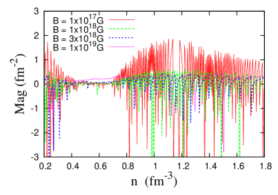
Figure 12: Magnetization as a function of the number density for the NJL model.

In Fig. 12 we show the magnetization of the system for different values of the magnetic field. As already discussed in ani and also seen in Fig. 1, the number of van alphen oscillations, related to the number of spikes in the NJL model, are larger for lower magnetic fields and decrease for stronger magnetic fields, when the number of filled Landau levels is small. Whenever $\mu_{f}=s_{f}$, i.e., whenever $B$ approaches a $n\neq 0$ Landau level, the denominator in Eq. (40) becomes zero and the contribution of this term to the magnetization of the system generates the spikes. This kind of contribution is not present in the MIT model and hence, the overall pattern is quite different in both models. Another important difference refers to the lack of oscillations in between 0.5 and 0.7 fm^-3 for all the fields within the NJL model. As pointed out in ani , this behavior is due to the $u$ and $d$ quark restoration of chiral symmetry and before the onset of the $s$ quark. Again, this behavior is not seen in the MIT model, where chiral symmetry effects are not present. Finally, it is worth mentioning that the MIT bag model only produces negative magnetization for very low magnetic fields while the NJL model gives negative values for the magnetization for all fields. Bearing in mind that negative magnetization refers to magnetic repulsion (diamagnetism) as opposed to positive magnetization that referes to magnetic attraction (paramagentism), the MIT and the NJL models show different physical pictures. We address this point again in the next section.

In Figs. 13, 14, 15 and 16, we show the anisotropic EOS with parallel and prependicular pressures without the inclusion of the $B^{2}$ term and in Figs. 17, 18, 19 and 20, the same EOS are plotted with the inclusion of this term. For $B=10^{17}$ G, the contribution of the $B^{2}$ term is almost negligible and hence, we can see that the magnetization already plays a role in the pressures, which are no longer coincident, as in the MIT model. As $B$ increases, the effects of the magnetization are clearly noticed. Once more, as in the MIT model, if the $B^{2}$ contribution is taken into account, the parallel pressure increases at lower energy densities and then decreases and goes to zero, reaching this point at lower values for larger magnetic fields. However, if one compares the isotropic pressure with the perpendicular pressure, they are just similar in average, since the magnetization effects are clearly present. This behavior is also quite different from the one exhibited by the MIT model and discussed in a previous section. Precisely because of the discontinuities in the perpendicular pressure, the anisotropic EOS cannot be used as input to the TOV equations.

At this point it is worth mentioning that similar calculations were perfomed in Huang_2015 for the NJL model with and without a vector interaction. However, in Huang_2015 the spikes in the EOS are not seem for fields as large as $4\times 10^{18}$ G . We have checked that if we plotted the pressure and energy density in MeV/fm³ (without the $B^{2}$ term) as in the mentioned reference, the spikes are almost imperceptible in the region of energy densities corresponding to 500-1000 MeV/fm³, but they are indeed present since they appear whenever $\mu_{f}=s_{f}$ in the denominator of Eq.(40). Notice also, that the parametrizaton of the electromagnetic interation in the EOS (exactly the $B^{2}$ term) is different in both papers, resulting in different quantitative results. If this term grows too rapidly the oscillation-free zone can dominate the equation of state.

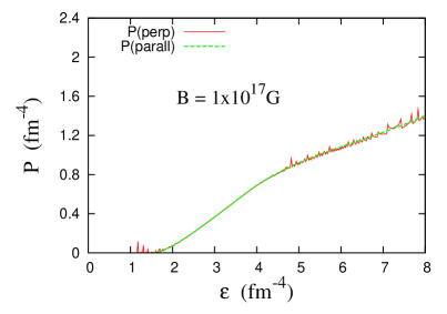
Figure 13: NJL model EOS obtained for $B=10^{17}$ G without the term proportional to $B^{2}$

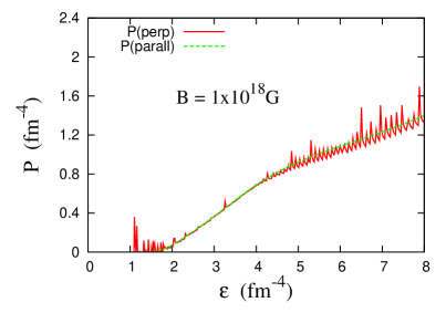
Figure 14: NJL model EOS obtained for $B=10^{18}$ G without the term proportional to $B^{2}$

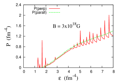
Figure 15: NJL model EOS obtained for $B=3\times 10^{18}$ G without the term proportional to $B^{2}$

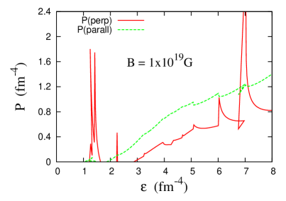
Figure 16: NJL model EOS obtained for $B=10^{19}$ G without the term proportional to $B^{2}$

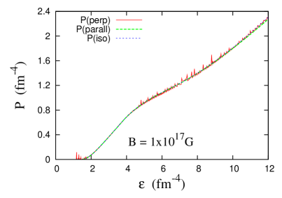
Figure 17: NJL model EOS obtained for $B=10^{17}$ G with the term proportional to $B^{2}$

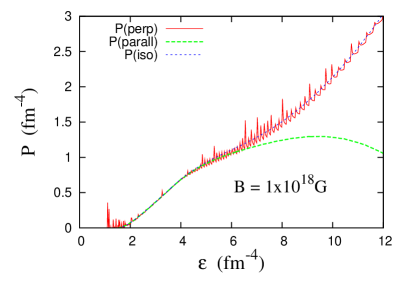
Figure 18: NJL model EOS obtained for $B=10^{18}$ G with the term proportional to $B^{2}$

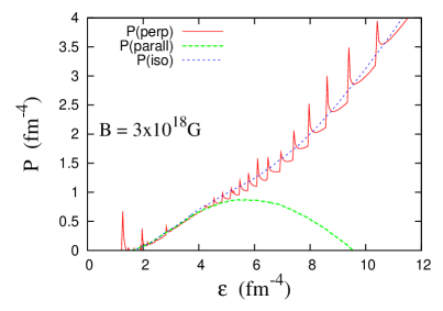
Figure 19: NJL model EOS obtained for $B=3\times 10^{18}$ G with the term proportional to $B^{2}$

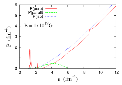
Figure 20: NJL model EOS obtained for $B=10^{19}$ G with the term proportional to $B^{2}$

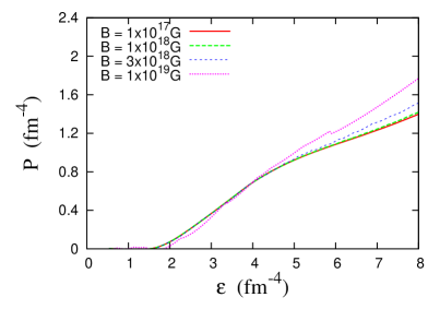
Figure 21: NJL EOS for different values of the chaotic magnetic field.

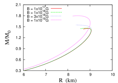
Figure 22: NJL model: Mass-radius relation within isotropic pressure for different values of magnetic field.

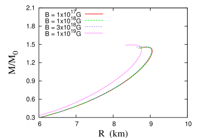
Figure 23: NJL model: Mass-radius relation within chaotic magnetic field approximation for different values of magnetic field.

Table 3: Properties of the maximum mass quark star

Model	$B$	$M_{max}$	$Mb_{max}$	R	${\cal E}_{c}$
	(G)	($M_{\odot}$)	($M_{\odot}$)	(km)	(fm-4)
NJLisotropic	$10^{17}$	1.45	1.53	8.93	7.51
NJLchaotic	$10^{17}$	1.45	1.53	8.92	7.66
NJLisotropic	$10^{18}$	1.46	1.54	8.87	7.76
NJLchaotic	$10^{18}$	1.45	1.53	8.92	7.46
NJLisotropic	$3.10^{18}$	1.55	1.62	8.44	9.58
NJLchaotic	$3.10^{18}$	1.47	1.54	8.85	7.86
NJLisotropic	$10^{19}$	1.80	1.77	8.42	10.25
NJLchaotic	$10^{19}$	1.49	1.49	8.51	8.93

Table 4: Properties of the 1.4$M_{\odot}$ quark star

Model	$B$	$M_{max}$	$Mb_{max}$	R	${\cal E}_{c}$
	(G)	($M_{\odot}$)	($M_{\odot}$)	(km)	(fm-4)
NJLisotropic	$10^{17}$	1.40	1.46	9.05	4.82
NJLchaotic	$10^{17}$	1.40	1.46	9.05	4.82
NJLisotropic	$10^{18}$	1.40	1.46	9.04	4.79
NJLchaotic	$10^{18}$	1.40	1.46	9.05	4.82
NJLisotropic	$3.10^{18}$	1.40	1.46	9.05	4.60
NJLchaotic	$3.10^{18}$	1.40	1.46	9.04	4.80
NJLisotropic	$10^{19}$	1.40	1.45	8.91	4.08
NJLchaotic	$10^{19}$	1.40	1.43	8.77	5.01

Finally, in Fig. 21, the EOS obtained with the chaotic formalism is shown for different values of the magnetic field. As the magnetic field increases the EOS becomes harder and within the NJL model, they are more sensible to the magnetic field than within the MIT model, where the EOSs just differ from each other for fields of the order of $10^{19}$ G, as seen in Fig. 8.

We then use the EOS obtained with the isotropic and chaotic formalisms to compute the stellar properties and the results are displayed in Figs 22, and 23 respectively, and in Table 3 we summarize the properties of the maximum mass quark star. As already expected, from the results existing in the literature prc2 , prc1 , the maximum stellar masses are very low, indicating that the NJL model cannot explain very massive magnetars. A solution to this setback is to include the vector interaction in the NJL model as in njlv . The overall conclusions coming out of the macroscopic properties for the NJL model are the same as the ones obtained with the MIT model, i.e., the maximum mass increases much more from a non-magnetized star to a strongly magnetized one if the isotropic formalism is used than if the chaotic field approximation is assumed.

Finally we display the properties of the canonical 1.4$M_{\odot}$ neutron stars in Table 4. We see that with the NJL, the quark star radii are very low, and are always in accordance with ref. webb , instead the constraints of ref. Steiner3 .

4 MIT versus NJL - differences

We start by reanalyzing the effects of the magnetization in the perpendicular pressure of both models. According to Eq. (16), the magnetization always comes multiplied by the magnetic field. We then plot, in Fig. 24 the term that really influences the perpendicular pressure for $B=3\times 10^{18}$ G. Theses results help us to understand the effects observed in Figs. 3 and 15 for the MIT and NJL models respectively. The term proportional to the magnetization is very small in both models and even when it becomes negative, the perpendicular pressure is not much smaller than the parallel one.

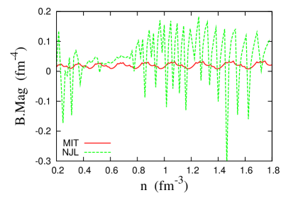
Figure 24: Magnetic field times the system magnetization for $B=3\times 10^{18}$ G for the MIT and the NJL models.

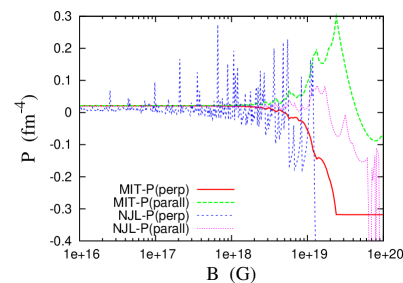
Figure 25: Anisotropic pressures for the MIT and the NJL without the $B^{2}$ contribution for $n=0.2n_{0}$.

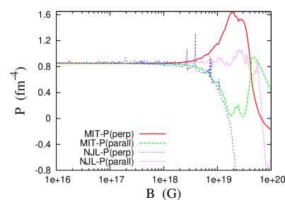
Figure 26: Anisotropic pressures for the MIT and the NJL without the $B^{2}$ contribution for $n=5n_{0}$.

Our last figures, Fig. 25 and Fig. 26, show the perpendicular and parallel pressures obtained from both models at a fixed densities, $0.2n_{0}$ and $5n_{0}$ with $n_{0}=0.16$ fm^-3 being the nuclear matter saturation density. These densities are chosen to represent stellar matter close to the crust and in the core of the star respectively. In these graphs the terms proportional do $B^{2}$ are not included. As shown in aurora1 for the MIT model, both pressures do not differ much up to a magnetic field of the order of $10^{18}$ G, when they start to deviate. For larger magnetic fields, of interest, for instance, in heavy ion collisions, the deviation first increases and then decreases again, stabilizing around $10^{20}$ G. For the NJL model, the behavior is not very different in average. For the case of lower density, the perpendicular pressure presents the typical spikes generated by the term that includes the magnetization and the parallel pressure is lower than the corresponding parallel pressure obtained with the MIT model, but the general trend is the same in both models. For $n=5n_{0}$, the number of spikes obtained with the NJL model decrease because this density corresponds to the region where the magnetization is very low, as shown in Fig. 12. One can see that the larger the density, the larger the differences between the pressures for fields higher than $10^{18}$G.

Another topic of interest is the effect of the magnetic field on the quark star radii. We can also see from Tables 2 and 4, that the NJL model always yields lower maximum masses and lower radii for the canonical 1.4$M_{\odot}$ NS. Comparing Figs. 9 and 11 with Figs. 22 and 23 we see that while the magnetic field increases the maximum mass in both MIT and NJL models, the effect on the radii is opposed. In both formalisms, isotropic and with chaotic field, for a fixed mass, the radii increase with the increase of the magnetic field in the MIT bag model and decrease in the NJL. In fact, the only case that produces a more compact quark star in the MIT bag model is when anisotropic pressure is considered. Unfortunately we are unable to calculate the TOV equation with the anisotopic NJL EOS due to the high oscillations in the pressure. Nevertheless, even if we could, these results would have to be taken with care since, as discussed in Section 2 because just one of the pressures is taken into account, since the other one becomes zero at still quite low densities. To trust macroscopic results obtained from a TOV-like equation, a self-consistent model for the study of the quark star structure such as the one proposed in Micaela should be done, so that more precise conclusions could be drawn.

5 Final remarks

In the present work we have used two models widely used to describe quark matter, the MIT and the NJL model and checked the effects of strong magnetic fields on their magnetization, EOS and stellar properties. To accomplish this task, we have revisited three formalisms generally applied to describe magnetized matter: the first one assumes that the EOS is isotropic, the second one that it is anisotropic and the third one that a chaotic field is possibly generated and maintained in the system.

For the second formalism, the calculation of the magnetization of the system is mandatory, since one of the pressures depends on this quantity. However, independently of the formalism used, the magnetization is a quantity that should be understood in a magnetized system. We have verified that both models produce quite different results. The NJL model presents three terms for the magnetization coming from the medium, the vacuum and the magnetic field itself. Just the first one is present in the MIT model and this explains most of the differences between both models.

As for the EOS, the isotropic and the chaotic formalisms present similar patterns in both models, the NJL being always slightly more sensible to the magnetic field strength. However, the anisotropic EOS shows a quite discontinuous behavior due to the spikes that appear in the calculation of the magnetization of the system.

When the macroscopic properties are computed, the isotropic EOSs always provide maximum stellar masses that are much larger than the ones obtained with a non-magnetized matter, in contrast with the values obtained with the chaotic field that do not result in much higher maximum masses. The small increase in the maximum masses is also found in more sophisticated calculations Mallick2 , Micaela .

Other important aspects related to quark matter subject to strong magnetic fields are the polarization and the viscosity of the system. For totally polarized matter, all particles lie on the lowest Landau level. The quark spin polarization has already been studied for both the MIT bag model in aurora1 and the NJL model in njlt , ani and hence, we only comment on the already known results. The polarization of the system increases with the increase of the magnetic field. In aurora1 , it is shown that the total polarization obtained with the MIT bag model occurs for $B\simeq 2\times 10^{19}$ G for matter in $\beta$-equilibrium. This result depends on the density and the temperature considered and is different for each quark flavor, since it depends on the charge of the quark njlt . For matter in $\beta$-equilibrium described by the NJL model, the electron becomes totally polarized for magnetic fields larger than $9\times 10^{17}$ G and the $s$ quark before $10^{18}$ G. The $u$ and $d$ quarks become totally polarized for approximately the same magnetic field as in the MIT bag model, i.e., higher than $10^{19}$ G and lower than $10^{20}$ G, the exact value being parameter dependent.

For quark matter, the non-leptonic processes

$$u+s\leftarrow u+d,\quad u+d\leftarrow u+s$$

are responsible for the restoration of chemical equilibrium and hence, they determine the bulk viscosity of the system. In sedrakian , bulk (and shear) viscosities are derived and discussed. Similar calculations remain to be done with the MIT bag model for the chaotic field approximation and for the NJL model and the results can shed some light on the stability of magnetized quark matter.

The physics of quark star radii is another open puzzle. It is well known that the radii of hadronic neutron stars are correlated with the symmetry energy slope $L$, horowitz , rafael , Gandolfi ,Constança ,Lopes3 . However we do not know yet if there is an analogue physical parameter that controls the quark star radius.

As mentioned in the Introduction, the influence of the quark AMM should not be completely disregarded. In chang2011 , it was shown that for quark matter the scale for the perturbative approach is defined by the constituent quark mass and therefore, the effects of the AMM should also be considered in the description of magnetized quark matter. As the quark mass is about one third the nucleon mass, the critical field will be approximately one order of magnitude smaller than the nucleon critical field, but still larger than the maximum field expected inside a quark star. Hence, the degeneracy of Landau levels will certainly be affected by the inclusion of the coupling between the field and the fermion anomalous magnetic moment. In a future work this problem should also be considered.

Before we conclude, it is important to stress that we have not exhausted the discussion on all formalisms since, as already mentioned in the Introduction, there are still other ones in the literature. One possible approach to deal with the anisotropic pressures and avoid the use of the TOV equations, is to follow the prescription used in Mallick2 with the help of the Hartle-Thorn method. We have seen that effects of the magnetization should not be disregarded as far as magnetic fields are stronger than $10^{17}$ G and hence, the calculations performed in Mallick2 , which completely ignore the contribution due to the magnetization of the system in the perpendicular pressure, should be revisited. There are also more sophisticated calculations that consider the anisotropy in solving Einstein’s field equations in a fully general relativistic formalism Bocquet ,Cardall ,Micaela , but the computational price paid is huge. Moreover, the fields generated at the surface of the star in Micaela are of the order of $10^{17}$ G, much higher than the $10^{15}$ G magnetic field expected in the surface of magnetars.

Acknowledgements D.P.M. acknowledges fruitful discussions with Marcus Benghi Pinto, Constança Providência and Verônica Dexheimer Strickland. This work was partially supported by Conselho Nacional de Desenvolvimento Científico e Tecnológico (CNPq-Brazil), CEFET/MG and by Fundação de Amparo à Pesquisa e Inovação do Estado de Santa Catarina (FAPESC-Brazil), under project 2716/2012.

References

- (1) J.B. Zirker, The Magnetic Universe, The Johns Hopkins University Press, Baltimore (2009).
- (2) R. Duncan and C. Thompson, Astrophysical Journal, Letters 392, (1992) L9; C. Kouveliotou et al, Nature 393, (1998) 235.
- (3) T. Inagaki, D. Kimura and T. Murata, Prog. Theo. Phys. 111, (2004) 371.
- (4) S.S. Avancini, D.P. Menezes, M.B. Pinto and C. Providência, Phys. Rev. D 85, (2012) 091901(R).
- (5) K. Fukushima, D. E. Kharzeev and H. J. Warringa, Phys. Rev. D 78 (2008) 074033; D. E. Kharzeev and H. J. Warringa, Phys. Rev. D 80, (2009) 034028; D. E. Kharzeev, Nucl. Phys. A 830, (2009) 543c.
- (6) K. Tuchin, Adv. High Energy Phys. 2013, (2013) 490495; Phys. Rev. C 88, (2013) 024911.
- (7) L. McLerran and V. Skokov, Nucl. Phys. A 929, (2014) 184.
- (8) A. Bzdak and V. Skokov, Phys. Lett. B 710, (2012) 171; W. -T. Deng and X. -G Huang, Phys. Rev. C 85, (2012) 044907.
- (9) M.G. de Paoli and D.P. Menezes, Adv. High Energy Phys. 2014, (2014) 479401.
- (10) G. Basar, D.E. Kharzeev and V. Skokov, Phys. Rev. Lett. 109, (2014) 202303; A.Bzdak and V. Skokov, Phys. Rev. Lett. 110, (2013) 192301.
- (11) P. Costa, M. Ferreira, H. Hansen, D. P. Menezes, C. Providência, Phys. Rev. D 89, (2014) 056013.
- (12) M. D’Elia, S. Mukherjee, and F. Sanfilippo, Phys. Rev. D 82, (2010) 051501.
- (13) E.-M. Ilgenfritz, M. Kalinowski, M. Müller-Preussker, B. Petersson, and A. Schreiber, Phys. Rev. D 85, (2012) 114504.
- (14) G. S. Bali, F. Bruckmann, G. Endrödi, Z. Fodor, S. D. Katz, S. Krieg, A. Schäfer, and K. K. Szabó, JHEP 1202, (2012) 044.
- (15) G. S. Bali, F. Bruckmann, G. Endrödi, Z. Fodor, S. D. Katz, S. Krieg, and A. Schäfer, Phys. Rev. D 86, (2012) 071502(R).
- (16) Ana G. Grunfeld, Debora P. Menezes, Marcus B. Pinto and Norberto Scoccola, Phys. Rev. D 90, (2014) 044024.
- (17) M. Ferreira, P. Costa, D.P. Menezes, C. Providência and N. Scoccola, Phys. Rev. D 89, (2014) 016002; M. Ferreira, P. Costa, O. Lourenço, T. Frederico, and C. Providência Phys. Rev. D 89, (2014) 116011.
- (18) R.L.S. Farias, K.P. Gomes, G. Krein and M.B. Pinto, Phys. Rev. C 90, (2014) 025203.
- (19) K. Fukushima and Y. Hidaka, Phys. Rev. Lett. 110, (2013) 031601; T. Kojo and N. Su, Phys. Lett. B 720, (2013) 192; F. Bruckmann, G. Endrodi, and T. G. Kovacs, JHEP 1304, (2013) 112; E.S. Fraga, J. Noronha, and L.F. Palhares, Phys. Rev. D 87, (2013) 114014.
- (20) D.Bandyopadhyay, S. Chakrabarty, S.Pal, Phys. Rev. Lett. 79, (1997) 2176.
- (21) G.J. Mao, C.J.Mao, A.Iwamoto, Z.X.Li, Chin, J. Astron. Astrophys. 3, (2003) 359.
- (22) A. Rabhi et al., J. Phys. G 36, (2009) 115204.
- (23) S.S. Avancini, D.P. Menezes, M.B. Pinto and C. Providência, Phys. Rev. C 80, (2009) 065805.
- (24) R. Casali, L.B. Castro and D.P. Menezes, Phys. Rev. C 89, (2014) 015805.
- (25) C.Y. Ryu, K.S. Kim, M.Ki Cheoun, Phys. Rev. C 82, (2010) 025804.
- (26) A.Rabhi, P.K. Panda, C. Providência, Phys. Rev. C 84, (2011) 035803.
- (27) R. Mallick, M. Sinha, Mon. Not. R. Astron. Soc. 414, (2011) 2702.
- (28) L.L. Lopes and D.P.Menezes, Braz. J. Phys. 42, (2012) 428.
- (29) V.Dexheimer, R. Negreiros, S. Schramm, Eur. J. Phys. A 48, (2012) 189.
- (30) Debora P. Menezes, Marcus B. Pinto, Luis R. B de Castro, Constança Providencia and Pedro Costa, Phys. Rev. C 89, (2014) 055207.
- (31) R. Mallick, S. Schramm, Phys. Rev. C 89, (2014) 045805.
- (32) R. O. Gomes, V. Dexheimer, C.A.Z. Vasconcellos, Astron. Nachr. 335, (2014) 666.
- (33) Luiz L. Lopes and Débora Peres Menezes, J. Cosmol. Astrop. Phys. 08 (2015) 002.
- (34) J. R. Oppenheimer and G. M. Volkoff, Phys. Rev. 55 (1939) 374.
- (35) N. Itoh, Prog. Theor. Phys., 44, (1970) 291.
- (36) A.R. Bodmer, Phys. Rev. D 4, (1971) 1601.
- (37) E. Witten, Phys. Rev. D 30, (1984) 272.
- (38) V. Dexheimer, J.R. Torres and D.P. Menezes, Eur. Phys. Jour. C 73 (2013) 2569.
- (39) E.J. Ferrer, V.de la Incera, J.P. Keith, I. Portillo and P.L. Springsteen, Phys. Rev. C 82, (2010) 065802.
- (40) J. L. Noronha and I. A. Shovkovy, Phys. Rev. D 76, 105030 (2007).
- (41) R. Gonzalez Felipe, A. Perez Martinez, H. Perez Rojas and M. Orsaria, Phys. Rev. C 77, (2008) 015807.
- (42) A. Rhabi, C. Providência and J. da Providência, J. Phys. G: Nucl Part. Phys. 35, (2008) 125201.
- (43) A. Broderick, M. Prakash, and J. M. Lattimer, Astrophys. J. 537, 351 (2000).
- (44) A. Chodos, R.L. Jaffe, K. Johnson, C.B. Thorne and V.F. Weisskopf, Phys. Rev, D 9, (1974) 3471.
- (45) Y. Nambu and G. Jona-Lasinio, Phys. Rev. 122 , (1961) 345; ibid. 124 , (1961) 246.
- (46) R.D. Blandford and L. Hernquist, J. Phys. C 15, (1982) 6233.
- (47) S. Chakrabarty, Phys. Rev. D 54, (1996) 1306.
- (48) A. Broderick, M. Prakash and J.M. Lattimer, Astrophys. J. 537, (2000), 351.
- (49) A. Rhabi et al, J. Phys. G: Nucl Part. Phys. 36, (2009) 115204.
- (50) D.P. Menezes, M. Benghi Pinto, S.S. Avancini, A. Pérez Martinez and C. Providência, Phys. Rev. C 79, (2009) 035807.
- (51) X. Huang, M. Huang, D.H. Rischke and A. Sedrakian, Phys. Rev. D 81, (2010) 045015.
- (52) L. Paulucci, E.J. Ferrer, V. de la Incera and J.E. Horvath, Phys. Rev. D 83, (2011) 043009.
- (53) D. Manreza Paret, J.E. Horvath and A. Perez Martinez, arXiv: 1407.2280[astro-ph.HE].
- (54) V. Dexheimer, D.P. Menezes and M. Strickland, J. Phys G 41, (2014) 015203.
- (55) M.Bocquet et al., Astr. & Astrophys. 301, (1995) 757.
- (56) C.Y. Cardall, M. Prakash, J.M. Lattimer, Astrophys. J. 554, (2011) 322.
- (57) C.W. Misner, Kip S. Thorne, J.A. Wheeler Gravitation, Freeman and Company, San Francisco (1973).
- (58) Ya.B. Zel’dovich, I.D. Nivikov, Stars and Relativity, Dover, New York (1996).
- (59) N. K. Glendenning, Compact Stars, Springer-Verlag, New-York, 2000.
- (60) J.R. Torres and D.P. Menezes, Eur. Phys. Lett. 102 (2013) 42003.
- (61) K. Hebeler, et al., Phys. Lett. 105 (2010) 161102.
- (62) A. W. Steiner, S. Gandolfi, Phys. Lett. 108 (2012) 081102.
- (63) A. W. Steiner, J. M. Lattimer, E. Brown, Astrophys. J 722 (2010) 33.
- (64) J. M. Lattimer, Y. Lim, Astrophys. J 771 (2013) 51.
- (65) S. Guillot, et al., Astrophys. J 772 (2013) 7.
- (66) A. W. Steiner, J. M. Lattimer Astrophys. J 784 (2014) 123.
- (67) Débora P. Menezes, Marcus B. Pinto and Constança Providência, Phys. Rev. C 91, (2015) 065205.
- (68) Peng-Cheng Chu, Xin Wang, Lie-Wen Chen and Mei Huang, Phys. Rev. D 91, (2015) 023003
- (69) T. Hatsuda and T. Kunihiro, Phys. Rep. 247, (1994) 221.
- (70) D. Chatterjee et al., arXiv:1410.6332v1 [astro-ph.HE]
- (71) S.S. Avancini, D.P. Menezes and C. Providência, Phys. Rev. C 83, (2011) 065805.
- (72) C.J. Horowitz and J. Piekarewicz, Phys. Rev. C 64, (2001) 062802; J. Carriere, C.J. Horowitz and J. Piekarewicz, AstroPhys. J. 593, (2003) 463.
- (73) R. Cavagnoli, D.P. Menezes and C. Providência, Phys. Rev. C 84, (2011) 065810.
- (74) S.Gandolfi, J. Carlson and S. Reddy, Phys. Rev. C 85, (2012) 032801(R).
- (75) C. Providência, Eur. Phys. J. A 50, (2014) 44.
- (76) L.L. Lopes and D.P.Menezes, Braz. J. Phys. 44, (2014) 774.
- (77) Lei Chang, Yu-Xin Liu, and Craig D. Roberts, Phys. Rev. Lett. 106, 072001 (2011).