Competing superconducting instabilities in the one-dimensional $\boldsymbol{p}$-band degenerate cold fermionic system

Abstract

The zero-temperature phase diagram of $p$-orbital two-component fermionic system loaded into a one-dimensional optical lattice is mapped out by means of analytical and numerical techniques. It is shown that the $p$-band model away from half-filling hosts various competing superconducting phases for attractive and repulsive interactions. At quarter filling, we analyze the possible formation of incompressible Mott phases and in particular for repulsive interactions, we find the occurrence of a Mott transition with the formation of fully gapped bond-ordering waves.

I Introduction

Ladder systems have been the focus of much theoretical and experimental work over more than two decades. One theoretical motivation was to investigate the dimensional crossover between the well-known one-dimensional (1D) physics and the two-dimensional (2D) case, in the search of 2D non-Fermi liquid physics. A second reason stems from experiments and the study of ladder compounds, such as the famous telephone number one Sr_14-xCa_xCu₂₄O₄₁ which has a superconducting phase at high pression and for a small hole density. dagotto

The simplest ladder model is that of a two-leg ladder, made of two coupled fermionic chains. In stark contrast to the single chain case, the two-leg ladder system displays a superconducting phase with $d$-wave superconductivity for repulsive interactions which stems from the doping of a spin-gapped Mott insulating phase at half-filling. bookboso; giamarchiThis gave the belief that the two-leg ladder problem already contains seeds of the rich physics of the cuprates.

Two-leg ladders have thus become over the years a fundamental system for the study of low-dimensional strongly correlated fermions. Various exotic quantum phases have been predicted theoretically depending on the form of the coupling between the two chains and the filling.larkin; fabrizio; rice; schulz2leg; fisher2leg; orignacdisorder; lin; schulzlast; furusaki; fradkin; lee; rvb1; fabrizio2005; marston; essler; nonnehund; shura Experimental realizations of two-leg ladder systems are clearly called for, in particular, to investigate the rich physics of the weak-coupling regime. In this respect, ultracold fermionic gases are a promising way to study two-leg ladder problems thanks to the high level of control on interchain hopping and interactions. lehur; lewenstein The ladder geometry might be created by considering double-well optical lattices for instance.anderlini; danshita; bloch

A second possible way is to load a two-component Fermi gas in a optical lattice and consider higher-lattice orbitals, typically the $p$-band, to simulate a fermionic two-leg ladder system. More precisely, we consider, in this paper, a two-component Fermi gas which is loaded in a 1D optical lattice (running along the $z$-direction) with moderate strength of (harmonic) confining potential $m\omega^{2}(x^{2}+y^{2})/2$ in the direction (i.e., $xy$) perpendicular to the chain. Kobayashi2012; Kobayashi2014; bois It is assumed that all the $s$-level of the oscillator are fully occupied while the $p$-level, i.e., $p_{x,y}$, are partially filled. The resulting lattice fermionic model has been derived in Refs. Kobayashi2012; Kobayashi2014; bois within the tight-binding approximation and takes the following form:

$$H_{p\textrm{-band}} = -t\sum_{i,m\alpha}\left(c_{m\alpha,\,i}^{\dagger}c_{m\alpha,\,i+1}+H.c.\right)$$ (1)

$$-~{}\mu\sum_{i}n_{i}+\frac{U_{1}+U_{2}}{4}\sum_{i}n_{i}^{2}$$

$$+~{}\sum_{i}\left[2U_{2}(T_{i}^{x})^{2}+(U_{1}-U_{2})(T_{i}^{z})^{2}\right],$$

where $m=p_{x},p_{y}$ is the orbital index and $\alpha=\>\uparrow,\downarrow$ is the ”spin” index or internal components of the underlying cold atoms. In Eq. (1), $n_{i}=\sum_{m\alpha}c_{m\alpha,\,i}^{\dagger}c_{m\alpha,\,i}$ describes the density operator at site $i$ and a pseudo-spin operator for the orbital degrees of freedom has been defined:

$$T_{i}^{a}=\frac{1}{2}c_{m\alpha,\,i}^{\dagger}\sigma^{a}_{mn}c_{n\alpha,\,i},$$ (2)

where $\sigma^{a},a=x,y,z$ are the Pauli matrices and a summation over repeated indices is implied. Model (1) can be viewed as a two-chain fermionic system without interchain hopping but with density-density interchain interactions and pair-hopping processes between the two orbitals (see Fig. 1).

Figure 1: (color online) The two-leg fermionic ladder representation of the $p$-band model (1). The orbital degrees of freedom plays the role of the legs of the ladder. Besides the kinetic term with amplitude $t$ for each orbital, there are local interactions at each site $i$: density-density intra-orbital (amplitude $U_{1}$, in red) and inter-orbital (amplitude $U_{2}$, in green), orbital exchange (amplitude $U_{2}$, in blue) and inter-orbital pair-hopping that breaks U(1)_o generically (amplitude $U_{2}$, in orange).

The continuous symmetry of model (1) for general $U_{1,2}$ is: $\text{U}(1)_{c}\times\text{SU}(2)_{s}$, where U(1)_c denotes the U(1) (charge) symmetry related to the conservation of the total number of atoms, while $\text{SU}(2)_{s}$ is the internal global SU(2) (spin) symmetry of the two-component Fermi gas. We note that the U(1)_o continuous symmetry for the orbital degrees of freedom is explicitly broken in Eq. (1). However, the use of harmonic potential in the $xy$ direction implies a constraint of the two coupling constants $U_{1,2}$ and the investigation of model (1) along the harmonic line $U_{1}=3U_{2}$ enjoys an U(1)_o symmetry corresponding to rotation along the $y$-axis in the orbital subspace. The U(1)_o symmetry is trivially realized when $U_{2}=0$ where the model reduces to two decoupled SU(2) Hubbard chains. Finally, the $U_{1}=U_{2}$ case displays also an U(1)_o symmetry since it is directly related to $U_{2}=0$ after a redefinition of the orbital pseudo-spin operator. We consider, in this paper, the most general case where $U_{1,2}$ are not fine-tuned for two main reasons. On the one hand, departure from the harmonic line $U_{1}=3U_{2}$ can be investigated by breaking the axial symmetry of the 2D harmonic trap with the introduction of quartic potentials. bois On the other hand, the harmonic line has been wrongly identified in Refs. Kobayashi2012; Kobayashi2014 and we want to make contact with their results obtained when $U_{2}=4U_{1}/9$.

At half-filling, it has been shown that model (1) along the harmonic line with repulsive interaction describes a Haldane phase haldane of the spin-1 Heisenberg chain. Kobayashi2012 The latter is known to be the paradigmatic 1D topological phase protected by symmetry.oshikawa For an attractive interaction, a Haldane phase for the charge degrees of freedom nonne2010; nonne2011 has also been predicted in Ref. Kobayashi2014 by means of a strong-coupling approach and density-matrix renormalization group (DMRG) calculations. white In Ref. bois, it has been shown that there is adiabatic continuity between weak and strong coupling regime and these two Haldane phases are related by a spin-charge interchange symmetry. The half-filled $p$-band model (1) along the harmonic line thus paves the way to realize experimentally non-trivial Haldane phases in the context of cold fermions.

In this paper, by means of a low-energy approach and DMRG calculations, we map out the zero-temperature phase diagram of the $p$-band model (1) for incommensurate filling and at quarter filling which best avoids three-body looses. In stark contrast to the conclusion of Ref. Kobayashi2014 for attractive interaction, we show that the $p$-band model (1) away from half-filling does not behave as an attractive 1D Hubbard chain with the formation of a 2$k_{F}$ CDW but instead is a representative of the physics of two-leg fermionic ladders. In particular, we find that the hallmark of its phase diagram is the emergence of various competing superconducting phases for attractive and repulsive interactions as well as a Mott transition with the formation of fully gapped bond-ordering waves (BOW).

The rest of the paper is organized as follows. In Sec. II, we present our low-energy approach based on a mapping onto Majorana fermions and a one-loop renormalization group (RG) analysis. A zero-temperature phase diagram for model (1) is then deduced in the weakly-interacting regime for incommensurate filling and at quarter filling with Fermi vector $k_{F}=\frac{\pi}{4a_{0}}$ ($a_{0}$ being the lattice spacing). In Sec. III, DMRG calculations are carried out to investigate the intermediate and large-coupling regimes to fully determine the phase diagram of the $p$-band model. We present then our concluding remarks in Sec. IV.

II The low-energy approach

In this section, we perform a weak-coupling approach to model (1) away from half-filling. We focus on incommensurate filling and a special commensurate filling where $k_{F}=\frac{\pi}{4a_{0}}$. The starting point of this approach is the introduction of left-right moving Dirac fermions from the continuum limit of the non-interacting Hamiltonian (1) with $U_{1,2}=0$:

$$c_{l\alpha,\,i}\rightarrow\sqrt{a_{0}}(L_{l\alpha}e^{-ik_{F}x}+R_{l\alpha}e^{ik_{F}x}),$$ (3)

with $x=ia_{0}$, $l=p_{x},p_{y}$, and $\alpha=\uparrow,\downarrow$. In stark contrast to the half-filled case of Ref. bois, there is a ”spin-charge” separation which strongly simplifies the analysis and the full Hamiltonian of the $p$-band model (1) decomposes into two commuting pieces:

$${\cal H}={\cal H}_{c}+{\cal H}_{s},$$ (4)

with $[{\cal H}_{c},{\cal H}_{s}]=0$, where ${\cal H}_{c}$ governs the physical properties of the charge degrees of freedom and ${\cal H}_{s}$ refers for all remaining non-Abelian degrees of freedom, i.e., spin, orbital and spin-orbital degrees of freedom.

II.1 Charge degrees of freedom

Let us first consider the simplest part in Eq. (4), i.e., the charge degrees of freedom. For incommensurate filling, on general grounds, the charge part takes the form of a Tomonaga-Luttinger Hamiltonian: bookboso; giamarchi

$${\cal H}_{c}=\frac{v_{c}}{2}\left[\frac{1}{K_{c}}\left(\partial_{x}\Phi_{c}\right)^{2}+K_{c}\left(\partial_{x}\Theta_{c}\right)^{2}\right],$$ (5)

where $v_{c}$ and $K_{c}$ are the Luttinger parameters. In this low-energy approach, the charge excitations are described by the bosonic field $\Phi_{c}$ and its dual field $\Theta_{c}$. The explicit form of the Luttinger parameters for the $p$-band model can be extracted from the continuum limit (3) after standard calculations. We find:

$$K_{c} = \frac{1}{\sqrt{1+g_{c}/\pi v_{F}}}$$

$$v_{c} = v_{F}\sqrt{1+g_{c}/\pi v_{F}},$$ (6)

where $v_{F}=2ta_{0}\sin(k_{F}a_{0})$ is the Fermi velocity and $g_{c}=2a_{0}(U_{1}+U_{2})$.

For incommensurate filling, no umklapp term appears and the charge degrees of freedom display metallic properties in the Luttinger liquid universality class. bookboso; giamarchi However, at quarter filling, umklapp processes might be generated leading to an additional term in Eq. (5). Such perturbation can be found by means of higher orders of the RG calculations or from lattice symmetries. OrignacCitro03 In this respect, the one-step translation symmetry expresses as follows in terms of the charge bosonic field: $T_{a_{0}}:\Phi_{c}\to\Phi_{c}+\sqrt{\pi/4}$ . The charge perturbation with the smallest scaling dimension which is compatible with the translation symmetry is then: ${\cal V}_{c}=-g_{u}\cos(\sqrt{16\pi}\Phi_{c})$. The full charge Hamiltonian density for the commensurate filling $k_{F}=\frac{\pi}{4a_{0}}$ becomes then equivalent to the quantum sine-Gordon model at $\beta^{2}=16\pi$:

$${\cal H}_{c}=\frac{v_{c}}{2}\left[\frac{1}{K_{c}}\left(\partial_{x}\Phi_{c}\right)^{2}+K_{c}\left(\partial_{x}\Theta_{c}\right)^{2}\right]-g_{u}\cos(\sqrt{16\pi}\Phi_{c}).$$ (7)

This model is exactly solvable and the development of the strong-coupling regime with a charge gap $\Delta_{c}$ corresponds to $K_{c}<1/2$, while for $K_{c}>1/2$ the charge degrees of freedom remain gapless in the Luttinger universality class. Using the estimate (6), we find the position of the critical line for a Mott transition within the bosonization approach:

$$U_{1c}+U_{2c}\simeq\frac{3\pi t\sqrt{2}}{2},$$ (8)

such that $K_{c}=1/2$. One has to be very careful with this estimate since the full expression of $K_{c}$ as a function of $U_{1,2}$ (6) is strictly valid only in the weak-coupling regime. One needs a complementary approach, i.e., numerical calculations to conclude on the existence or not of a Mott transition for the lattice model (1). Note that the mechanism of the Mott transition is very similar to the one which occurs in the repulsive U(4) Hubbard chain assaraf99; rey or in the problem of spin-3/2 cold fermions. Lecheminant2005; phle; Sylvain2007; Roux2009

For $K_{c}<1/2$, the charge degrees of freedom are fully gapped and the strong-coupling regime of the sine-Gordon model (7) is described by the pinning of the charged field on the minima:

$$\langle\Phi_{c}\rangle = p\sqrt{\pi/4},\;g_{u}>0$$

$$\langle\Phi_{c}\rangle = \left(p+\frac{1}{2}\right)\sqrt{\pi/4},\;g_{u}<0,$$ (9)

$p$ being an integer. The sign of the umklapp coupling constant $g_{u}$ is difficult to fix but we expect $g_{u}<0$ from an higher-order perturbative expansion in the weak-coupling regime so that:$\langle\Phi_{c}\rangle=\frac{\sqrt{\pi}}{4}$. OrignacCitro03 The DMRG calculations of Sec. III will shed light on the position of the pinning of the charge field from the determination of the Mott-insulating phases of the $p$-band model. The low-lying excitations are massive kinks and antikinks which interpolate between the ground states of the quantum sine-Gordon model (7). The charges associated to these charge excitations are

$$Q=\pm\frac{2}{\sqrt{\pi}}\int\mathrm{d}x\;\partial_{x}\Phi_{c}=\pm 1,$$ (10)

in units of the electron charge. We have thus massive holon as low-lying excitations in the charge sector.

II.2 Non-Abelian sector

The low-energy physics of the remaining degrees of freedom, included in ${\cal H}_{\rm s}$ of Eq. (4), can be inferred from a mapping onto six Majorana fermions as in Refs. lee; rvb1; fabrizio2005; Azaria99; Boulat

A simple way to obtain this correspondence is through the introduction of four chiral bosonic fields $\Phi_{l\sigma R,L},l=p_{x},p_{y};\sigma=\>\uparrow,\downarrow$ from the bosonization of Dirac fermions:bookboso; giamarchi

$$R_{\,l\sigma} = \frac{\kappa_{l\sigma}}{\sqrt{2\pi a_{0}}}\exp{\left(i\sqrt{4\pi}\Phi_{l\sigma R}\right)}$$

$$L_{l\sigma} = \frac{\kappa_{l\sigma}}{\sqrt{2\pi a_{0}}}\exp{\left(-i\sqrt{4\pi}\Phi_{l\sigma L}\right)},$$ (11)

where the bosonic fields satisfy the following commutation relation:

$$\left[\Phi_{l\sigma R},\Phi_{l^{\prime}\sigma^{\prime}L}\right]=\frac{i}{4}\delta_{ll^{\prime}}\delta_{\sigma\sigma^{\prime}}.$$ (12)

The presence of the Klein factors $\kappa_{l\sigma}$ ensures the correct anticommutation of the fermionic operators. The Klein factors satisfy the anticommutation rule $\{\kappa_{l\sigma},\kappa_{l^{\prime}\sigma^{\prime}}\}=2\delta_{ll^{\prime}}\delta_{\sigma\sigma^{\prime}}$ and they are constrained so that $\Gamma^{2}=1$, with $\Gamma=\kappa_{p_{x}\uparrow}\kappa_{p_{x}\downarrow}\kappa_{p_{y}\uparrow}\kappa_{p_{y}\downarrow}$. Hereafter, we will work within the $\Gamma=1$ sector.

The next step of the approach is to introduce a bosonic basis which singles out the different degrees of freedom, i.e., charge, spin, orbital, and spin-orbital degrees of freedom:Azaria99

$$\Phi_{p_{x}\uparrow L,R}=\frac{1}{2}\big{(}\Phi_{c}+\Phi_{s}+\Phi_{o}+\Phi_{so}\big{)}_{L,R}$$

$$\Phi_{p_{x}\downarrow L,R}=\frac{1}{2}\big{(}\Phi_{c}-\Phi_{s}+\Phi_{o}-\Phi_{so}\big{)}_{L,R}$$

$$\Phi_{p_{y}\uparrow L,R}=\frac{1}{2}\big{(}\Phi_{c}+\Phi_{s}-\Phi_{o}-\Phi_{so}\big{)}_{L,R}$$

$$\Phi_{p_{y}\downarrow L,R}=\frac{1}{2}\big{(}\Phi_{c}-\Phi_{s}-\Phi_{o}+\Phi_{so}\big{)}_{L,R}.$$ (13)

From these new bosonic fields, one can now consider a refermionization procedure by introducing six left and right moving Majorana fermions through:

$$\xi_{L}^{2}+i\xi_{L}^{1}=\frac{\eta_{1}}{\sqrt{\pi a_{0}}}\exp{\Big{(}-i\sqrt{4\pi}\Phi_{sL}\Big{)}}$$

$$\xi_{R}^{2}+i\xi_{R}^{1}=\frac{\eta_{1}}{\sqrt{\pi a_{0}}}\exp{\Big{(}i\sqrt{4\pi}\Phi_{sR}\Big{)}}$$

$$\xi_{L}^{4}-i\xi_{L}^{5}=\frac{\eta_{2}}{\sqrt{\pi a_{0}}}\exp{\Big{(}-i\sqrt{4\pi}\Phi_{oL}\Big{)}}$$

$$\xi_{R}^{4}-i\xi_{R}^{5}=\frac{\eta_{2}}{\sqrt{\pi a_{0}}}\exp{\Big{(}i\sqrt{4\pi}\Phi_{oR}\Big{)}}$$

$$\xi_{L}^{6}+i\xi_{L}^{3}=\frac{\eta_{3}}{\sqrt{\pi a_{0}}}\exp{\Big{(}-i\sqrt{4\pi}\Phi_{soL}\Big{)}}$$

$$\xi_{R}^{6}+i\xi_{R}^{3}=\frac{\eta_{3}}{\sqrt{\pi a_{0}}}\exp{\Big{(}i\sqrt{4\pi}\Phi_{soR}\Big{)}},$$ (14)

where $\eta_{1,2,3,4}$ are again Klein factors which ensure the adequate anticommutation rules for the fermions. Using this correspondence, the interacting part of ${\cal H}_{\rm s}$ can be expressed in terms of these Majorana fermions:

$${\cal H}^{\rm int}_{s}=\frac{\lambda_{1}}{2}\left(\sum_{a=1}^{3}\xi^{a}_{R}\xi^{a}_{L}\right)^{2}+\lambda_{2}\left(\sum_{a=1}^{3}\xi^{a}_{R}\xi^{a}_{L}\right)\xi^{4}_{R}\xi^{4}_{L}$$

$$+~{}\lambda_{3}\left(\sum_{a=1}^{3}\xi^{a}_{R}\xi^{a}_{L}\right)\xi^{6}_{R}\xi^{6}_{L}+\lambda_{4}\left(\sum_{a=1}^{3}\xi^{a}_{R}\xi^{a}_{L}\right)\xi^{5}_{R}\xi^{5}_{L}$$

$$+~{}\lambda_{5}\xi^{5}_{R}\xi^{5}_{L}\xi^{6}_{R}\xi^{6}_{L}+\lambda_{6}\xi^{4}_{R}\xi^{4}_{L}\xi^{5}_{R}\xi^{5}_{L}+\lambda_{7}\xi^{4}_{R}\xi^{4}_{L}\xi^{6}_{R}\xi^{6}_{L},$$ (15)

with the identification:

$$\begin{array}[]{lll}\lambda_{1}&=&-a_{0}(U_{1}+U_{2})\\ \lambda_{2}&=&-2a_{0}U_{2}\\ \lambda_{3}&=&a_{0}(U_{2}-U_{1})\\ \lambda_{4}&=&0\\ \lambda_{5}&=&2a_{0}U_{2}\\ \lambda_{6}&=&a_{0}\left(U_{1}-U_{2}\right)\\ \lambda_{7}&=&0.\end{array}$$

Using standard calculations, the one-loop RG equations for model (15) can de derived:

$$\dot{\lambda}_{1} = \frac{1}{2\pi}\lambda_{1}^{2}+\frac{1}{2\pi}\lambda_{2}^{2}+\frac{1}{2\pi}\lambda_{3}^{2}+\frac{1}{2\pi}\lambda_{4}^{2}$$

$$\dot{\lambda}_{2} = \frac{1}{\pi}\lambda_{1}\lambda_{2}+\frac{1}{2\pi}\lambda_{3}\lambda_{7}+\frac{1}{2\pi}\lambda_{4}\lambda_{6}$$

$$\dot{\lambda}_{3} = \frac{1}{\pi}\lambda_{1}\lambda_{3}+\frac{1}{2\pi}\lambda_{2}\lambda_{7}+\frac{1}{2\pi}\lambda_{4}\lambda_{5}$$

$$\dot{\lambda}_{4} = \frac{1}{\pi}\lambda_{1}\lambda_{4}+\frac{1}{2\pi}\lambda_{2}\lambda_{6}+\frac{1}{2\pi}\lambda_{3}\lambda_{5}$$

$$\dot{\lambda}_{5} = \frac{3}{2\pi}\lambda_{3}\lambda_{4}+\frac{1}{2\pi}\lambda_{6}\lambda_{7}$$

$$\dot{\lambda}_{6} = \frac{3}{2\pi}\lambda_{2}\lambda_{4}+\frac{1}{2\pi}\lambda_{5}\lambda_{7}$$

$$\dot{\lambda}_{7} = \frac{3}{2\pi}\lambda_{2}\lambda_{3}+\frac{1}{2\pi}\lambda_{5}\lambda_{6}.$$ (16)

As often in 1D, the RG equations enjoy some hidden discrete symmetries:

$$\Omega_{1} : \lambda_{2,3,4}\rightarrow-\lambda_{2,3,4}$$

$$\Omega_{2} : \lambda_{2,6,7}\rightarrow-\lambda_{2,6,7}$$

$$\Omega_{3} : \lambda_{4,5,6}\rightarrow-\lambda_{4,5,6}$$

$$\Omega_{4} : \lambda_{3,5,7}\rightarrow-\lambda_{3,5,7},$$ (17)

which correspond to the existence of duality symmetries on the Majorana fermions Boulat

$$\Omega_{1} : \xi^{1,2,3}_{L}\rightarrow-\xi^{1,2,3}_{L}$$

$$\Omega_{2} : ~{}~{}\xi^{4}_{L}~{}~{}\,\rightarrow-\xi^{4}_{L}$$

$$\Omega_{3} : ~{}~{}\xi^{5}_{L}~{}~{}\,\rightarrow-\xi^{5}_{L}$$

$$\Omega_{4} : ~{}~{}\xi^{6}_{L}~{}~{}\,\rightarrow-\xi^{6}_{L}\,\,,$$ (18)

while the right-moving Majorana fermions remain invariant. These chiral transformations for each Majorana fermion correspond, in the continuum limit, to the well-known Kramers-Wannier duality symmetry of the underlying 1D Ising model in a transverse field. The latter transformation maps the ordered phase to the disorder one which is ordered in terms of the disorder operator. bookboso Starting from the ordered phase of the six underlying Ising models in a transverse field, the transformations (18) lead then to four possible different gapful phases. A numerical RG analysis of Eqs. (16) is necessary to determine which phases is indeed reached starting from the initial conditions (II.2).

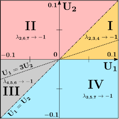
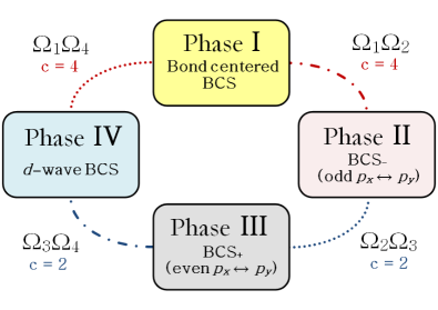
Figure 2: (color online) Top: Numerical phase diagram obtained by the one-loop RG analysis of Eq. (16). Bottom: For each phase denoted I-IV, we give the dominant superconducting correlations (see text) as well as the duality symmetries which relate the phases between them. We display the central charge $c=2$ or $c=4$ which characterizes the different quantum phase transitions of the model.

We did this numerical analysis and, as depicted in Fig. (2), it reveals that the RG flow goes in the strong-coupling regime in the far infrared (IR) along four asymptotic lines:

$$I:\; \lambda_{2}=\lambda_{3}=\lambda_{4}=-\lambda_{5}=-\lambda_{6}=-\lambda_{7}=-\lambda_{1}$$

$$II:\; \lambda_{2}=-\lambda_{3}=-\lambda_{4}=-\lambda_{5}=\lambda_{6}=\lambda_{7}=-\lambda_{1}$$

$$III:\; \lambda_{2}=\lambda_{3}=-\lambda_{4}=-\lambda_{5}=-\lambda_{6}=\lambda_{7}=\lambda_{1}$$

$$IV:\; \lambda_{2}=-\lambda_{3}=\lambda_{4}=-\lambda_{5}=\lambda_{6}=-\lambda_{7}=\lambda_{1}.$$ (19)

Along these rays, the interacting part of the effective Hamiltonian (15) simplifies as follows:

$$\Omega_{1} : \mathcal{H}^{\Omega_{1}}_{\text{int}}=\frac{g}{2}\left(\sum_{a=4}^{6}\xi^{a}_{R}\xi^{a}_{L}-\sum_{a=1}^{3}\xi^{a}_{R}\xi^{a}_{L}\right)^{2}$$

$$\Omega_{2} : \mathcal{H}^{\Omega_{2}}_{\text{int}}=\frac{g}{2}\left(\sum_{a\neq 4}\xi^{a}_{R}\xi^{a}_{L}-\xi^{4}_{R}\xi^{4}_{L}\right)^{2}$$

$$\Omega_{3} : \mathcal{H}^{\Omega_{3}}_{\text{int}}=\frac{g}{2}\left(\sum_{a\neq 5}\xi^{a}_{R}\xi^{a}_{L}-\xi^{5}_{R}\xi^{5}_{L}\right)^{2}$$

$$\Omega_{4} : \mathcal{H}^{\Omega_{4}}_{\text{int}}=\frac{g}{2}\left(\sum_{a\neq 6}\xi^{a}_{R}\xi^{a}_{L}-\xi^{6}_{R}\xi^{6}_{L}\right)^{2},$$ (20)

with $g>0$. Using the duality symmetries (18), all these models reduces to the same model which takes the form of the SO(6) Gross-Neveu (GN) model with interaction: GN

$${\cal H}^{\rm int}_{\rm GN} = \frac{g}{2}\left(\sum_{a=1}^{6}\xi^{a}_{R}\xi^{a}_{L}\right)^{2}.$$ (21)

This is an example of a dynamical symmetry enlargement (DSE) where an SO(6) symmetry, i.e. a higher symmetry than the initial symmetry of the $p$-band lattice model, emerges at low-energy. This phenomenon occurs in a large variety of models with marginal interactions in the scaling limit saleur as, for instance, in the half-filled two-leg Hubbard model lin and in the SU(4) Hubbard chain at half-filling assaraf, where an SO(8) symmetry occurs at low energy. The emergence of an SO(6) symmetry has also been obtained within the one-loop RG analysis of various models of doped two-leg ladders. schulzlast; lee; rvb1; essler; Boulat

II.3 Phases of the $p$-band model

The main interest of this SO(6) DSE scenario stems from the fact that the isotropic RG ray is described by a massive integrable field theory (21) when $g>0$. zamolo; karowski The development of the strong-coupling regime in the SO(6) model leads to generation of a non-perturbative fermionic mass, i.e. the emergence of a spin-gap phase where all spin, orbital and spin-orbital excitations are fully gapped. The nature of the underlying electronic phases of the $p$-band model can then be inferred by a straightforward semiclassical approach of the SO(6) model and the application of the duality symmetries (18). Alternatively, one can perform a direct bosonic semiclassical approach of the different models in Eq. (20) using the identification (14). In the following, we proceed to this analysis by identifying the phases of Fig. 2.

II.3.1 Phase I: $\Omega_{1}$ duality

In the first phase, when $U_{1}>0$ and $U_{1}>U_{2}$ of Fig. (2), the numerical analysis of the one-loop RG equations reveals that the RG flow is attracted in the far IR along a special ray (I) of Eq. (19). This phase is described by the $\Omega_{1}$ duality and the resulting physical properties of that phase are governed by the interacting Hamiltonian $\mathcal{H}^{\Omega_{1}}_{\text{int}}$ of Eq. (20). A straightforward semiclassical approach of the latter model leads to the following pinning of the bosonic fields:

$$\langle\Phi_{s}\rangle=0,\;\;\langle\Phi_{o}\rangle=\frac{\sqrt{\pi}}{2},\;\;\langle\Theta_{so}\rangle=0.$$ (22)

The electronic properties of phase I, which includes the harmonic line $U_{1}=3U_{2}$, depend also on the charge degrees of freedom that are decoupled.

Let us first consider the $K_{c}>1/2$ case. One has then a gapless charge excitation whereas all remaining spin, orbital, and spin-orbital excitations are fully gapped. All $2k_{F}$ densities are short-ranged due to the pinning of the dual spin-orbital field $\Theta_{so}$. Interestingly enough, the leading electronic instability in this phase turns out to be a bond-centered superconducting instability with order parameter:

$${\cal O}_{\tiny{\mbox{BCSbond}}}=c_{p_{x}\uparrow,i+1}c_{p_{y}\downarrow,i}-c_{p_{x}\downarrow,i+1}c_{p_{y}\uparrow,i}-(p_{x}\leftrightarrow p_{y}),$$ (23)

which is odd under the $\mathbb{Z}_{2}$ orbital exchange symmetry ($p_{x}\leftrightarrow p_{y}$). A similar superconducting instability has been introduced in the study of doped two-leg electronic ladder in Ref. Robinson2012. In the continuum limit, we have:

$${\cal O}_{\tiny{\mbox{BCSbond}}} \simeq a_{0}2i\sin(k_{F}a_{0})\big{(}R_{p_{x}\uparrow}L_{p_{y}\downarrow}+R_{p_{y}\downarrow}L_{p_{x}\uparrow}$$

$$~{}~{}~{}~{}~{}~{}~{}~{}~{}~{}~{}~{}~{}~{}~{}~{}~{}~{}~{}~{}~{}~{}~{}-~{}R_{p_{x}\downarrow}L_{p_{y}\uparrow}-R_{p_{y}\uparrow}L_{p_{x}\downarrow}\big{)}.$$

One can then bosonize this operator by means of the identification (11) and the physical basis (13):

$${\cal O}_{\tiny{\mbox{BCSbond}}} \simeq \frac{4\sin(k_{F}a_{0})}{\pi}\kappa_{p_{x}\uparrow}\kappa_{p_{y}\downarrow}e^{-i\sqrt{\pi}\Theta_{c}}$$

$$\times\big{[}-i\sin\sqrt{\pi}\Phi_{s}\cos\sqrt{\pi}\Phi_{o}\sin\sqrt{\pi}\Theta_{so}$$

$$~{}~{}~{}~{}~{}+~{}\cos\sqrt{\pi}\Phi_{s}\sin\sqrt{\pi}\Phi_{o}\cos\sqrt{\pi}\Theta_{so}\big{]}.$$

Taking account of the vacuum expectation values (22), we get ${\cal O}_{\tiny{\mbox{BCSbond}}}\simeq e^{-i\sqrt{\pi}\Theta_{c}}$ so that the equal-time correlation function of the pairing operator has a power-law decay:

$$\langle{\cal O}^{\dagger}_{\tiny{\mbox{BCSbond}}}\left(x\right){\cal O}_{\tiny{\mbox{BCSbond}}}\left(0\right)\rangle\sim x^{-1/2K_{c}}.$$ (26)

When $1/2<K_{c}<1$, the bond-centered BCS superconducting instability is strongly enhanced with respect to the non-interacting case. We have thus a dominant superconducting instability for repulsive interaction.

While the $2k_{F}$ densities are short-ranged in phase I, $4k_{F}$ densities might compete with the superconducting instability (23). Many $4k_{F}$ density terms can be written in the continuum description like $\rho^{(1)}_{4k_{F}}\sim\sum_{l\sigma}L^{\dagger}_{l\sigma}R_{l\sigma}L^{\dagger}_{l-\sigma}R_{l-\sigma}$ for instance. The latter gives in the bosonized language:

$$\rho^{(1)}_{4k_{F}}\sim e^{i\sqrt{4\pi}\Phi_{c}}\cos\sqrt{4\pi}\Phi_{o},$$ (27)

so that in the spin-gapped phase (22), one has $\rho^{(1)}_{4k_{F}}\sim e^{i\sqrt{4\pi}\Phi_{c}}$, and therefore a power-law decay for its correlation function:

$$\langle\rho^{(1)\dagger}_{4k_{F}}\left(x\right)\rho^{(1)}_{4k_{F}}\left(0\right)\rangle\sim x^{-2K_{c}}.$$ (28)

Since $K_{c}>1/2$, one observes that the $4k_{F}$ density correlation function (28) decays much faster than the superconducting one (26). In summary, the leading instability of phase I with $K_{c}>1/2$ is the bond-centered BCS superconducting one.

In the Mott-insulating phase with $K_{c}<1/2$, all excitations are fully gapped. The bond-centered BCS superconducting instability (23) is now short-ranged since the charge field $\Phi_{c}$ is pinned (9) and thus its dual field $\Theta_{c}$ is a strongly fluctuating field. In contrast, the $4k_{F}$ density of Eq. (27) can have now a non-zero expectation value, breaking spontaneously the translation symmetry. We thus expect a Mott phase with a two-fold degenerate ground state at quarter filling $k_{F}=\frac{\pi}{4a_{0}}$. The nature of this phase depends on the sign of the coupling constant $g_{u}$ of the umklapp perturbation in model (7). In this respect, we introduce the following order parameters as in the study of the extended quarter-filled two-leg Hubbard ladder: OrignacCitro03

$${\cal O}_{\rm BOW_{\pi,q_{y}}}\!(i) = \left(-1\right)^{i}\sum_{\sigma}\Big{(}c^{\dagger}_{p_{x}\sigma,i+1}c_{p_{x}\sigma,i}$$

$$~{}~{}~{}~{}~{}~{}~{}~{}~{}~{}~{}~{}~{}~{}+\cos q_{y}\;c^{\dagger}_{p_{y}\sigma,i+1}c_{p_{y}\sigma,i}+H.c.\Big{)}$$

$${\cal O}_{\rm CDW_{\pi,q_{y}}}\!(i) = \left(-1\right)^{i}\sum_{\sigma}\Big{(}c^{\dagger}_{p_{x}\sigma,i}c_{p_{x}\sigma,i}$$ (29)

$$~{}~{}~{}~{}~{}~{}~{}~{}~{}~{}~{}~{}~{}~{}+\cos q_{y}\;c^{\dagger}_{p_{y}\sigma,i}c_{p_{y}\sigma,i}\Big{)},$$

with $q_{y}=0,\pi$. One can obtain a continuum and bosonized representation for these order parameters. The $4k_{F}$ contribution of the latter plays a crucial role and can be derived using the results of Refs. Haldane4kf; Schulz93; OrignacCitro03 and we get for the leading contribution:

$$(-1)^{i}\sum_{\sigma}c^{\dagger}_{l\sigma,i+1}c_{l\sigma,i}+H.c.\sim\sin\sqrt{4\pi}(\Phi_{c}+\epsilon_{l}\Phi_{o})$$

$$(-1)^{i}\sum_{\sigma}c^{\dagger}_{l\sigma,i}c_{l\sigma,i}\sim\cos\sqrt{4\pi}(\Phi_{c}+\epsilon_{l}\Phi_{o}),$$ (30)

with $\epsilon_{p_{x}}=1$, $\epsilon_{p_{y}}=-1$. From these results, we find the bosonized descriptions of the order parameters (29):

$${\cal O}_{\rm BOW_{\pi,\pi}} \sim \cos\sqrt{4\pi}\Phi_{c}\sin\sqrt{4\pi}\Phi_{o}$$

$${\cal O}_{\rm BOW_{\pi,0}} \sim \sin\sqrt{4\pi}\Phi_{c}\cos\sqrt{4\pi}\Phi_{o}$$

$${\cal O}_{\rm CDW_{\pi,\pi}} \sim \sin\sqrt{4\pi}\Phi_{c}\sin\sqrt{4\pi}\Phi_{o}$$

$${\cal O}_{\rm CDW_{\pi,0}} \sim \cos\sqrt{4\pi}\Phi_{c}\cos\sqrt{4\pi}\Phi_{o}.$$ (31)

Taking into account that in phase I, we have $\langle\Phi_{o}\rangle=\sqrt{\pi}/2$, we have either a uniform $4k_{F}$ BOW or uniform $4k_{F}$ CDW depending on the sign of the umklapp term in Eq. (7):

$$\langle{\cal O}_{\rm BOW_{\pi,0}}\rangle \neq 0,\;\;{\rm if}\;\;g_{u}<0$$

$$\langle{\cal O}_{\rm{CDW}_{\pi,0}}\rangle \neq 0,\;\;{\rm if}\;\;g_{u}>0.$$ (32)

We expect in the weak-coupling regime that $g_{u}<0$. A uniform $4k_{F}$ BOW is thus stabilized which is two-fold degenerate and breaks the translation symmetry. The latter phase is similar to the BOW phase obtained in the quarter-filled spin-3/2 SO(5) chain model. Sylvain2007

II.3.2 Phase II: $\Omega_{2}$ duality

In the second phase, when $U_{2}>0$ and $U_{1}<U_{2}$, the one-loop RG flow is now attracted in the far IR by the asymptote (II) of Eq. (19). This phase is described by the $\Omega_{2}$ duality. A straightforward semiclassical approach of model $\mathcal{H}^{\Omega_{2}}_{\text{int}}$ in Eq. (20) leads to the following pinning of the bosonic fields in this phase:

$$\langle\Phi_{s}\rangle=0,\;\;\langle\Theta_{o}\rangle=0,\;\;\langle\Phi_{so}\rangle=0.$$ (33)

In this phase, as we will see in Sec. III, numerical results find that $K_{c}>1/2$. All spin, orbital, and spin-orbital excitations are fully gapped in this phase and the charge degrees of freedom are gapless since $K_{c}>1/2$. Due to the presence of attractive interactions, one may call this gapless phase a Luther-Emery phase as in the spin-1/2 Hubbard chain with $U<0$. bookboso; giamarchi Its physical nature is very different from that of phase I since the expectation values of the bosonic fields (33) are different. As it can readily be seen from Eq. (33), we have again the condensation of a dual field, here the orbital one $\Theta_{o}$, which implies that the $2k_{F}$-CDW operator is a strongly fluctuating order. As in phase I, the only possible CDW quasi-long range order in this phase is a $4k_{F}$ CDW. However, the $\rho^{(1)}_{4k_{F}}$ CDW of Eq. (27) becomes now short-range since the orbital dual field $\Theta_{o}$ condenses in phase II. In this respect, we have to consider another $4k_{F}$ CDW instability: $\rho^{(2)}_{4k_{F}}\sim\sum_{\sigma}L^{\dagger}_{p_{x}\sigma}R_{p_{x}\sigma}L^{\dagger}_{p_{y}\sigma}R_{p_{y}\sigma}$. The latter can be directly expressed in terms of the bosonic field:

$$\rho^{(2)}_{4k_{F}}\sim e^{i\sqrt{4\pi}\Phi_{c}}\cos\sqrt{4\pi}\Phi_{s}.$$ (34)

Using the expectation values (33), we deduce the leading asymptotics of the equal-time correlation function of the $4k_{F}$ CDW operator:

$$\langle\rho^{(2)\dagger}_{4k_{F}}\left(x\right)\rho^{(2)}_{4k_{F}}\left(0\right)\rangle\sim x^{-2K_{c}}.$$ (35)

As it will be seen in the next section, we have $K_{c}>1/2$ and, one does not expect, on general ground, that this $4k_{F}$-CDW will be the dominant instability in this phase. As in phase I, a superconducting instability turns out to be the leading one. The latter is defined by the following order parameter:

$${\cal O}_{\rm BCS-}=c_{p_{x}\uparrow,i}c_{p_{x}\downarrow,i}-c_{p_{y}\uparrow,i}c_{p_{y}\downarrow,i},$$ (36)

which is odd under the $\mathbb{Z}_{2}$ orbital symmetry ($p_{x}\leftrightarrow p_{y}$) and antisymmetric with respect to the spin degrees of freedom ($\uparrow\leftrightarrow\downarrow$). The order parameter (36) can be expressed directly in terms of the bosonic fields:

$${\cal O}_{\rm BCS-} \simeq \frac{2\kappa_{p_{x}\uparrow}\kappa_{p_{x}\downarrow}}{\pi}e^{-i\sqrt{\pi}\Theta_{c}}$$

$$\times\Big{[}\cos\sqrt{\pi}\Phi_{s}\cos\sqrt{\pi}\Theta_{o}\cos\sqrt{\pi}\Phi_{so}$$

$$~{}+i\sin\sqrt{\pi}\Phi_{s}\sin\sqrt{\pi}\Theta_{o}\sin\sqrt{\pi}\Phi_{so}\Big{]}.$$

Using the expectation values (33), we get ${\cal O}_{\rm BCS-}\simeq e^{-i\sqrt{\pi}\Theta_{c}}$, so that the equal-time correlation function of the pairing operator (36) has a power-law decay:

$$\langle{\cal O}^{\dagger}_{\rm BCS-}\left(x\right){\cal O}_{\rm BCS-}\left(0\right)\rangle\sim x^{-1/2K_{c}},$$ (38)

which dominates the $4k_{F}$ CDW ones (35) when $K_{c}>1/2$.

II.3.3 Phase III: $\Omega_{3}$ duality

The next phase, defined by $U_{2}<0$ and $U_{1}<U_{2}$, is described by the asymptote (III) of the one-loop RG flow. The harmonic line of the $p$-band model with attractive interaction belongs to this phase which is described by the $\Omega_{3}$ duality with interacting Hamiltonian $\mathcal{H}^{\Omega_{3}}_{\text{int}}$ of Eq. (20). The bosonic fields of the bosonization approach are now pinned to the values:

$$\langle\Phi_{s}\rangle=0,\;\;\langle\Theta_{o}\rangle=\frac{\sqrt{\pi}}{2},\;\;\langle\Phi_{so}\rangle=0.$$ (39)

A spin-gap is formed and a gapless $c=1$ phase emerges in this attractive regime with $U_{1,2}<0$ since the umklapp term cannot gap out the charge degrees of freedom when $K_{c}>1$. In close parallel to the previous cases, one can determine the nature of the leading electronic instability of this Luther-Emery phase by means of the bosonization approach combined with the pinning (39). The dominant $4k_{F}$ CDW is the one of phase II, given by Eq. (34) with the power-law behavior (35). The relevant superconducting instability for phase III is defined by:

$${\cal O}_{\rm BCS+}=c_{p_{x}\uparrow,i}c_{p_{x}\downarrow,i}+c_{p_{y}\uparrow,i}c_{p_{y}\downarrow,i},$$ (40)

which is even under the $\mathbb{Z}_{2}$ orbital symmetry ($p_{x}\leftrightarrow p_{y}$) and antisymmetric with respect to the spin degrees of freedom ($\uparrow\leftrightarrow\downarrow$). In terms of the bosonic fields, it reads as follows:

$${\cal O}_{\rm BCS+} \simeq -\frac{2\kappa_{p_{x}\uparrow}\kappa_{p_{x}\downarrow}}{\pi}e^{-i\sqrt{\pi}\Theta_{c}}$$

$$\times\Big{[}i\cos\sqrt{\pi}\Phi_{s}\sin\sqrt{\pi}\Theta_{o}\cos\sqrt{\pi}\Phi_{so}$$

$$~{}~{}+\phantom{i}\sin\sqrt{\pi}\Phi_{s}\cos\sqrt{\pi}\Theta_{o}\sin\sqrt{\pi}\Phi_{so}\Big{]}.$$

Using the vacuum expectation values (39), we immediately get ${\cal O}_{\rm BCS+}\simeq e^{-i\sqrt{\pi}\Theta_{c}}$, so that the equal-time correlation function of this pairing operator has a power-law decay:

$$\langle{\cal O}^{\dagger}_{\rm BCS+}\left(x\right){\cal O}_{\rm BCS+}\left(0\right)\rangle\sim x^{-1/2K_{c}}.$$ (42)

Since $K_{c}>1$, we conclude that the superconducting instability (40) dominates the $4k_{F}$-CDW ordering (35). The Luther-Emery phase is thus governed by a superconducting instability (40) in stark contrast to the $2k_{F}$-CDW phase predicted by the DMRG study of Ref. Kobayashi2014. The physics of the $p$-band model with attractive interaction is thus not similar to that of 1D attractive Hubbard model as emphasized in Ref. Kobayashi2014.

II.3.4 Phase IV: $\Omega_{4}$ duality

The last phase of the $p$-band model corresponds to the region where $U_{2}<0$ and $U_{1}>U_{2}$. The numerical analysis of the RG flow shows that, here, the one-loop RG flow is attracted in the far IR by the special line (IV) of Eq. (19). The resulting phase is described by the $\Omega_{4}$ duality with interacting Hamiltonian $\mathcal{H}^{\Omega_{4}}_{\text{int}}$ of Eq. (20) which leads to the following pinning for the bosonic fields of the bosonization approach:

$$\langle\Phi_{s}\rangle=0,\;\;\langle\Phi_{o}\rangle=0,\;\;\langle\Theta_{so}\rangle=0.$$ (43)

As before, this pinning leads to the formation of a gapless $c=1$ phase when $K_{c}>1/2$ where the charge degrees are the only critical modes of the problem. We now consider the standard $d$-wave superconducting instability of the two-leg electronic ladder to determine the nature of phase IV:

$${\cal O}_{\rm BCSd}=c_{p_{x}\uparrow,i}c_{p_{y}\downarrow,i}-c_{p_{x}\downarrow,i}c_{p_{y}\uparrow,i},$$ (44)

which is even under the $\mathbb{Z}_{2}$ orbital symmetry ($p_{x}\leftrightarrow p_{y}$). The bosonized expression of this superconducting instability reads as follows:

$${\cal O}_{\rm BCSd} \simeq \frac{2\kappa_{p_{x}\uparrow}\kappa_{p_{y}\downarrow}}{\pi}e^{-i\sqrt{\pi}\Theta_{c}}$$

$$\times\Big{[}i\sin\sqrt{\pi}\Phi_{s}\sin\sqrt{\pi}\Phi_{o}\sin\sqrt{\pi}\Theta_{so}$$

$$+\cos\sqrt{\pi}\Phi_{s}\cos\sqrt{\pi}\Phi_{o}\cos\sqrt{\pi}\Theta_{so}\Big{]}.$$

From this expression, we observe that this operator is a fluctuating order, i.e., has short-ranged correlation, in the previous phases, while, in phase IV, one has from the pinning (43): ${\cal O}_{\rm BCSd}\sim e^{-i\sqrt{\pi}\Theta_{c}}$. The $d$-wave superconducting instability (44) becomes dominant in phase IV with the power-law behavior:

$$\langle{\cal O}^{\dagger}_{\rm BCSd}\left(x\right){\cal O}_{\rm BCSd}\left(0\right)\rangle\sim x^{-1/2K_{c}}.$$ (46)

From the pinning (43), we find that the $2k_{F}$-CDW operator is short-ranged while the $4k_{F}$ CDW of phase II, given by Eq. (34), has a power-law behavior in phase IV:

$$\langle\rho^{(2)\dagger}_{4k_{F}}\left(x\right)\rho^{(2)}_{4k_{F}}\left(0\right)\rangle\sim x^{-2K_{c}},$$ (47)

with subleading exponent when $K_{c}>1/2$ with respect to the superconducting instability (46).

II.3.5 Quantum phase transitions

From the duality symmetries (18), we can, as well, discuss the different quantum phase transitions that occur in the $p$-band model by investigating self-dual manifolds. However, Fig. 2 reveals that the transitions belong to special lines of the lattice model: $U_{1}=U_{2}$ and $U_{2}=0$. From Eq. (1), the $U_{2}=0$ describes two decoupled quarter-filled spin-1/2 Hubbard chains with $U_{1}$ coupling constant. When $U_{1}<0$, a spin-gap is formed and therefore the phase II/phase III transition is critical with $c=1+1=2$ gapless charge modes. When $U_{1}>0$, all degrees of freedom are gapless since the quarter-filled spin-1/2 Hubbard chains is known not to exhibit a Mott transition. giamarchi The phase I/phase IV transition is thus critical with central charge $c=4$. The transition between phase I and phase II is located along the $U_{1}=U_{2}>0$ line of the $p$-band model. From the definition of the $p$-band model (1), one can show that the latter line corresponds to two decoupled repulsive quarter-filled spin-1/2 Hubbard chains which does not have relevant umklapp process. A $c=4$ behavior should occur along this quantum phase transition. Finally, the last transition between phase III and phase IV belongs to the $U_{2}=U_{1}<0$ line which takes the form of two decoupled attractive quarter-filled spin-1/2 Hubbard chains with a $c=2$ quantum critical behavior. All these results can be derived by investigating self-dual manifolds of the RG Eqs. (16). Since the transition lines are located on special high symmetry lines, one would expect the location of these transitions to remain universal beyond the weak coupling regime where this analysis is valid. This will be indeed confirmed numerically in Sec. III.2. A summary of the phases and quantum phase transitions, obtained from the low-energy approach, can be found in the bottom of Fig. 2.

III DMRG calculations

III.1 Determination of the phase diagram

We will now determine the phase diagram of the $N=2$ $p$-band model at quarter filling (i.e. 1 particle per site) using numerical simulations with the DMRG algorithm. This will allow to go beyond the one-loop RG analysis done in Fig. 2 and check the analytical predictions for realistic intermediate or strong couplings $(U_{1},U_{2})$ (we fix $t=1$ as the unit of energy). Moreover, numerical data are needed to determine the numerical value of the Luttinger parameter $K_{c}$ which allows to compute the dominant correlations.

Typically, we have used open boundary conditions (OBC) and lengths $L=64$ and $L=128$, keeping up to 4000 states when computing correlations in order to keep a discarded weight below $10^{-10}$ in most regions, although simulations where $0\leq U_{2}\leq U_{1}$ were found to be more difficult to converge (discarded weight around $10^{-7}$, see discussion below). For practical purpose, we have mapped the $p$-band model onto an equivalent (pseudo)spin-1/2 (where the pseudo spin corresponds to the orbital) fermionic models on a $2$-leg ladder, and we have implemented the abelian U(1) symmetry corresponding to the conservation of particles spin.

Our main result is presented in Fig. 3 where we plot the phase diagram vs $(U_{1}/t,U_{2}/t)$ obtained by computing various correlation functions on $L=128$ systems. We will present the numerical data below, but we can already discuss the different phases. First of all, the (quantum phase) transition lines are found to be $U_{2}=0$ and $U_{1}=U_{2}$, which is expected by symmetry since they correspond to special lines of the model, see Sec. II.3.5. A detailed analysis will be given in Sec. III.2. Second, it is remarkable that phases II, III and IV found in the weak-coupling analysis are confirmed to exist in a wide range of parameters. Last, we have computed the Luttinger parameter $K_{c}$ using the dominant correlation, which is always of some BCS type, in each of these phases.

Overall, we observe a rather good agreement between the numerical phase diagrams obtained by solving RG equations (Fig. 2) or the full microscopic model using DMRG (Fig. 3), except for the large Mott phase at this commensurate filling. For incommensurate filling, we predict that the RG phase diagram would be identical to the numerical one.

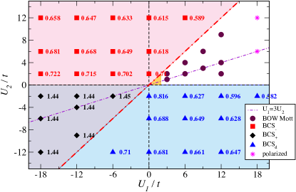
Figure 3: (color online) Numerical phase diagram obtained by DMRG simulations with length $L=128$. Numerical values correspond to the Luttinger parameter $K_{c}$ in each region.

We will now present some numerical data that were used to compute this numerical phase diagram. We have relied mostly on computing superconducting correlation functions (in various channels) as well as density ones. To avoid spurious effects due to OBC, we have chosen to compute correlations as

$$C_{\cal O}(x)=\langle{\cal O}^{\dagger}(L/4+x){\cal O}(L/4)\rangle$$ (48)

so that we can determine if they decay algebraically or are short-ranged. In Figs. 4-5-6, such correlations are plotted and correspond respectively to phases II, III and IV. In all cases, we emphasize that dominant correlations are found to be the superconducting ones, in different channels (see below). Indeed, the Luttinger parameter $K_{c}$ is always larger than 1/2 in the critical phases, otherwise a Mott phase is stabilized. Some values of $K_{c}$ are given on the phase diagram in Fig. 3. In particular, for phases II, III and IV, we observe an adiabatic continuity from weak to strong coupling, while phase I on the contrary is much reduced and replaced instead by Mott phase at intermediate coupling and polarization at strong coupling.

III.1.1 Phase II

In this region of the phase diagram, our numerical results, shown in Fig. 4 for instance when $U_{1}/t=-6$ and $U_{2}/t=6$, are in perfect agreement with the RG predictions and dominant BCS_- predictions. However, numerics is needed to compute the Luttinger parameter $K_{c}$ and determine whether pairing correlations dominate over density ones. Using Eqs. (35)-(38), our numerical fits for both BCS_- and CDW correlations are compatible with a single $K_{c}>1/2$, for instance 0.65 for the parameters set chosen on the plot. All the other correlations are short-ranged as expected. The leading instability in this phase is therefore the BCS_- superconducting one.

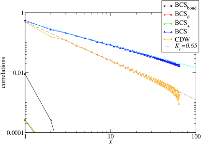
Figure 4: (color online) Absolute values of correlation functions (see text) vs distance for ($U_{1}/t=-6$, $U_{2}/t=6$) and $L=128$ obtained with DMRG. This corresponds to our phase II. Fitting the dominant BCS_- correlation with Eq. (38) leads to $K_{c}=0.65$, which is also consistent with the $4k_{F}$ CDW correlation function (see Eq. (28)).

III.1.2 Phase III

The phase III region is particularly interesting since it could be achieved experimentally using the harmonic trapping scheme (i.e. $U_{1}=3U_{2}$) with attractive interactions. As seen in Fig. 5, we have found that the dominant correlations are of the pairing type, in the BCS₊ channel. In all this region, they can be fitted using Eq. (42) to get $K_{c}>1$ (values are given in the phase diagram). In such a case, the dominant density correlations are uniform and decay as $1/x^{2}$ as expected.

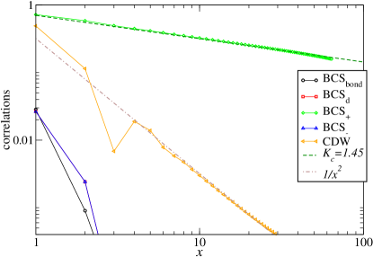
Figure 5: (color online) Absolute values of correlation functions (see text) vs distance along the harmonic line in the attractive case ($U_{1}/t=-6$, $U_{2}/t=-2$) for $L=128$ obtained with DMRG. This corresponds to our phase III. Fitting the dominant BCS₊ correlation with Eq. (42) leads to $K_{c}=1.45$.

Note that this dominant superconducting correlation function was not computed in Ref. Kobayashi2014, where only CDW signal was discussed. As a result, the dominant instability in this Luther-Emery phase is a superconducting one, in stark contrast to the $2k_{F}$-CDW phase predicted earlier Kobayashi2014.

III.1.3 Phase IV

In the region corresponding to phase IV, our numerical results in Fig. 6 indicate that dominant correlations are of the pairing type again, but in a different BCS_d channel, as expected from the low-energy analysis. In the whole region, we can fit these correlations using Eq. (46) to extract $K_{c}$, or equivalently we could fit the subleading CDW correlations with Eq. (47), although it would be less precise. Some values of $K_{c}$ are given in Fig. 3 and are always larger than 1/2 so that no Mott transition is found.

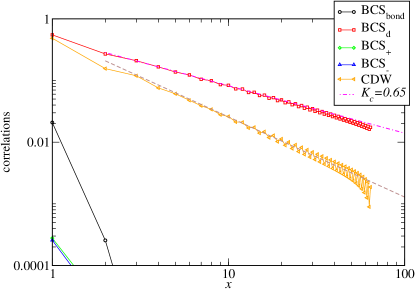
Figure 6: (color online) Absolute values of correlation functions (see text) vs distance for ($U_{1}/t=6$, $U_{2}/t=-6$) and $L=128$ obtained with DMRG. This corresponds to our phase IV. Fitting the dominant BCS_d correlation with Eq. (46) leads to $K_{c}=0.65$, which is also consistent with the $4k_{F}$ CDW correlation function (see Eq. (28)).

III.1.4 Phase I

The region $0<U_{1}<U_{2}$, which should correspond to phase I (see Fig. 2) according to RG solution is more involved to analyze. We have plotted on Fig. 7 the finite-size scaling of the $(\pi,0)$ BOW, i.e. the kinetic energy difference measured in the middle of the chain. Data are given along the harmonic line $U_{1}=3U_{2}$. Extrapolations are compatible with a finite, albeit small, value for intermediate interactions (for instance $U_{1}=6$, $U_{2}=2$), while it seems to vanish in the weak and strong coupling regimes. It is known that the weak coupling is difficult numerically since the non-interacting starting point correspond to two decoupled fermionic chains with a large total central charge $c=4$. For instance, the Mott transition in the SU($N$) Hubbard model at filling $1/N$ has been discussed quite extensively to occur for a finite critical $(U/t)_{c}$ when $N>2$ based on bosonization and quantum Monte-Carlo results assaraf99 as well as DMRG ones rey, while some older DMRG simulations had indicated a vanishing $U_{c}=0$ Buchta2007. Since the charge gap is expected to open in an exponentially way, this is clearly a difficulty for any numerical technique. However, this regime is perfectly suited for bosonization and weak-coupling RG: indeed, since the Luttinger parameter $K_{c}=1$ in the non-interacting case, umklapp processes are irrelevant so that finite interactions are necessary to enter the Mott phase.

Thus, our interpretation is the following: (i) for small interaction parameters, RG analysis should be valid and phase I with dominant BCS_bond correlations is expected with $K_{c}>1/2$ so that umklapp processes are irrelevant; (ii) for intermediate interactions, a Mott phase occurs with $(\pi,0)$ BOW and exponentially decaying BCS correlations at large distance; (iii) for very large interactions (i.e. $U_{1}=18$ and $U_{2}=6$), we have noticed that the ground-state is ferromagnetically polarized (hence degenerate): the polarized ground-state can be simply understood as two decoupled spinless fermionic chains (one for each orbital), which energy is independent of both $U_{1}$ and $U_{2}$. Intuitively, such a state could be stabilized at large $U$’s since other competing states will have higher energies. Still, our numerics is clear on this point as can be checked by comparing ground-state energies in different sectors (varying the number of particles per spin), or measuring $K_{c}=1$ from charge correlations (data not shown).

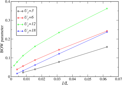
Figure 7: (color online) Finite-size scaling of the $(\pi,0)$ BOW order parameter along the harmonic line $U_{1}=3U_{2}$.

III.2 Nature of the phase transitions

A simple way to obtain information on the phases, or on their phase transitions, is through the measurements of block von Neumann entanglement entropy which is known to scale as Calabrese-C-04:

$$S_{\text{vN}}=(c/6)\log d(x|L)+\mathrm{Cst}$$ (49)

where $c$ is the central charge and $d(x|L)=(L/\pi)\sin(\pi x/L)$ the conformal distance. On a finite system with OBC, due to Friedel oscillations, the fitting can be more involved and one can use for instance the knowledge of the local kinetic bond energies to get more reliable results (see Fig. 11 of Ref. Roux2009 for instance). Our numerical results should be compared to the analytical predictions made in Sec. II.3.5.

In Fig. 8(a), we have plotted typical data in phases II, III and IV. By removing oscillations using the bond kinetic energy as an additional fitting parameter, we can obtain smooth functions that perfectly agree with the expected behavior (49) with $c=1$.

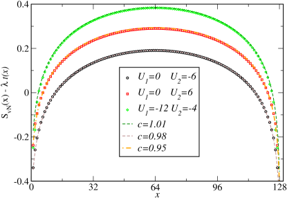
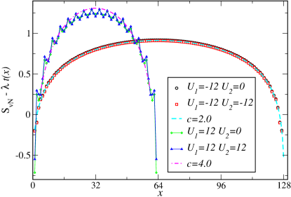
Figure 8: (color online)(a) Block entanglement entropies vs size $x$ obtained for $L=128$ and various $(U_{1},U_{2})$. Oscillations have been removed using the bond kinetic energies $t(x)$ and fitting parameter $\lambda$ (equal respectively to $2$, $1.25$ and $2.4$ (see text). In all cases, we can extract a central charge $c\simeq 1$ as expected. (b) Similar data along the quantum phase transitions which can be fitted with $c=2.0$ (using $\lambda=0.325$) in the attractive case and with $c=4.0$ (using $\lambda=1.5$ and $1$, plus a shift for clarity) in the repulsive case using smaller $L=64$ system.

Now, considering the expected quantum phase transition along the lines $U_{1}=U_{2}$ and $U_{2}=0$, we can clearly identify different behaviors for attractive vs repulsive interactions (as expected since there will be a finite spin gap or not respectively). In Fig. 8(b) for attractive interactions, we can fit our entanglement entropies data perfectly with $c=2$ using $L=128$. In the repulsive case, our numerical data are not converged on the same size keeping up to $m=8000$ states, so that we plot instead data obtained with $L=64$ and $m=8000$. In this case, we cannot remove entirely the oscillations in the data, but we can get a very good fit using the expected $c=4$ central charge. Overall, we get an excellent agreement with the theoretical predictions.

IV Conclusion

We have presented a comprehensive study of the most general model relevant for one-dimensional $p$-band two-component fermionic cold gases with local interactions only. We have concentrated here on incommensurate filling and quarter-filling. 

Using a state-of-the-art low-energy approach, supplemented with a one-loop RG numerical analysis, we have found that generically, the charge sector decouples from the spin-orbital one which is gapped. As a consequence, most of the phase diagram is occupied by standard Luttinger liquid phases with a single gapless charge mode (hence a central charge $c=1$). Nevertheless, we have clarified the nature of the dominant instability and have found that it is always of some BCS superconducting kind, in one of the following channels: BCS_bond, BCS_-, BCS₊ and BCS_d, see Eqs. (23)-(36)-(40)-(44) respectively. In particular, an interesting bond-centered superconducting instability emerges along the harmonic line for the repulsive interaction. The nature of the phase transitions between these four superconducting phases is also elucidated and found to behave with central charges $c=2$ or $c=4$.

Our numerical simulations do confirm that phases with dominant BCS_-, BCS₊ and BCS_d extend from weak to strong coupling and occupy large regions in the phase diagram. In particular, for attractive interactions and harmonic trapping, BCS₊ correlations are the dominant ones, different from the $2k_{F}$-CDW phase predicted earlier Kobayashi2014. In the last region where the bond-centered superconducting instability BCS_bond is expected at weak coupling, our DMRG data at quarter-filling (i.e., one particle per site) indicate that a Mott phase intervene with fully gapped bond-ordering waves at intermediate coupling, and spontaneous polarization at strong coupling. We have also numerically confirmed the nature of all the quantum phase transitions present in this model.

The $p$-band two-component fermion mode, studied in this paper, is thus an interesting model to explore superconducting instabilities of doped two-leg fermionic ladder systems as well as the occurence of a Mott transition. Given the recent progress in realizing SU($N$)-symmetric Fermi gases CazalillaRey; review, we hope that some of the phases discussed here could be realized experimentally and probed using local spectroscopy techniques or by measuring short-range correlations.