Doctor of Philosophy School of Mathematical Sciences Faculty of Science B.Sc.(Hons), M.Sc.

Simulating Astrophysical Magnetic Fields with Smoothed Particle Magnetohydrodynamics

Copyright Notice

Under the Copyright Act 1968, this thesis must be used only under the normal conditions of scholarly fair dealing. In particular no results or conclusions should be extracted from it, nor should it be copied or closely paraphrased in whole or in part without the written consent of the author. Proper written acknowledgement should be made for any assistance obtained from this thesis.

I certify that I have made all reasonable efforts to secure copyright permissions for third-party content included in this thesis and have not knowingly added copyright content to my work without the owner’s permission.

Summary

Numerical methods to improve the treatment of magnetic fields in smoothed field magnetohydrodynamics (SPMHD) are developed and tested. A mixed hyperbolic/parabolic scheme is developed which “cleans” divergence error from the magnetic field. The method introduces a scalar field which is coupled to the magnetic field. A conservative form for the hyperbolic equations is obtained by first defining the energy content of the new field, then using it in the discretised Lagrangian to obtain equations which manifestly conserve energy. This is shown to require conjugate first derivative operators in the SPMHD cleaning equations. Average divergence error is shown to be an order of magnitude lower for all test cases considered, and allows for the stable simulation of the gravitational collapse of magnetised molecular cloud cores. The effectiveness of the cleaning may be improved by explicitly increasing the hyperbolic wave speed or by cycling the cleaning equations between timesteps. In the latter, it is possible to achieve $\nabla\cdot{\bf B}=0$ in SPMHD. The method is adapted to work with a velocity field, demonstrating that it can reduce density variations in weakly compressible SPH simulations by a factor of 2.

A switch to reduce dissipation of the magnetic field from artificial resistivity is developed. Discontinuities in the magnetic field are located by monitoring jumps in the gradient of the magnetic field at the resolution scale relative to the magnitude of the magnetic field. This yields a simple yet robust method to reduce dissipation away from shocked regions. Compared to the existing switch in the literature, this leads to sharper shock profiles in shocktube tests, lower overall dissipation of magnetic energy, and importantly, is able to capture magnetic shocks in the highly super-Alfvénic regime.

These numerical methods are compared against grid-based MHD methods by comparison of the small-scale dynamo amplification of a magnetic field in driven, isothermal, supersonic turbulence. We use the SPMHD code, Phantom, and the grid-based code, Flash. We find that the growth rate of Flash is largely insensitive to the numerical resolution, whereas Phantom shows a resolution dependence that arises from the scaling of the numerical dissipation terms. The saturation level of the magnetic energy in both codes is about $2$–$4\%$ of the mean kinetic energy, increasing with higher magnetic Reynolds numbers. Phantom requires lower resolution to saturate at the same energy level as Flash. The time-averaged saturated magnetic spectra have a similar shape between the two methods, though Phantom contains twice as much energy on large scales. Both codes have PDFs of magnetic field strength that are log-normal, which become lopsided as the magnetic field saturates. We find encouraging agreement between grid- and particle methods for ideal MHD, concluding that SPMHD is able to reliably simulate the small-scale dynamo amplification of magnetic fields. We note that quantitative agreement on growth rates can only be achieved by including explicit, physical terms for viscosity and resistivity, because those are the terms that primarily control the growth rate and saturation level of the turbulent dynamo.

Declaration of Published Material

In accordance with Monash University Doctorate Regulation 17.2 Doctor of Philosophy and Research Master s regulations the following declarations are made:

I hereby declare that this thesis contains no material which has been accepted for the award of any other degree or diploma at any university or equivalent institution and that, to the best of my knowledge and belief, this thesis contains no material previously published or written by another person, except where due reference is made in the text of the thesis.

This thesis includes 3 original papers published in or submitted to peer reviewed journals and 2 unpublished conference proceedings. The ideas, development and writing up of all the papers in the thesis were the principal responsibility of myself, the candidate, working within the School of Mathematical Sciences under the supervision of Dr. Daniel Price.

The inclusion of co-authors reflects the fact that the work came from active collaboration between researchers and acknowledges input into team-based research.

I have renumbered sections of submitted or published papers in order to generate a consistent presentation within the thesis.

The following chapters and/or sections have appeared in conference proceedings, have been published in peer reviewed journals, or have been submitted for publication:

• Sections 3.2–3.4, 3.7, and Appendix A appear in
  Tricco, T. S. and Price, D. J.: 2012, ‘Constrained hyperbolic divergence cleaning for smoothed particle magnetohydrodynamics’. J. Comput. Phys. 231, 7214–7236.

• Section 3.6 appears in
  Tricco, T. S. and Price, D. J.: 2012, ‘Hyperbolic divergence cleaning for SPH’. Proceedings of the 7th International SPHERIC Workshop.

• Sections 4.1, 4.2, and 4.4 appear in
  Tricco, T. S. and Price, D. J.: 2013, ‘A switch to reduce resistivity in smoothed particle magnetohydrodynamics’. MNRAS 436, 2810–2817.

• Section 4.3 appears in
  Tricco, T. S. and Price, D. J.: 2013, ‘A switch for artificial resistivity and other dissipation terms’, Proceedings of the 8th International SPHERIC Workshop.

• Chapter 5 and Appendices B and C to appear in
  Tricco, T. S., Price, D. J., and Federrath, C.: 2014, ‘A comparison between grid and particle methods on small-scale dynamo amplification of magnetic fields in supersonic turbulence’, Submitted to ApJ.

Acknowledgments

I remember the moment I realised I should go to Australia. I enjoyed working with SPMHD and thought there was a lot of room for innovation in that area. At first I hadn’t considered doing a Ph.D. outside of Canada, but then the decision became obvious — I had been reading primarily the work of Daniel Price, and he seemed like a good guy: I should do my Ph.D. with him.

Moving to Melbourne in general has really been an positive influence on my life. I’ve thoroughly enjoyed my time at Monash, in Melbourne, and in Australia. I have had more opportunities for my Ph.D. than I could have hoped for, and I have made a lot of great friends and had great experiences. I’m sad to see this chapter of my life coming to a close.

I first and foremost sincerely wish to thank my supervisor, Daniel Price. He has been an incredible teacher, and there are many anecdotes I would like to share to demonstrate that, but then this would end up becoming very long. Suffice to say, he has really taught me a lot — directly and indirectly — on what takes to be a good researcher. The support, encouragement, and understanding that he has given me exceeded what I could have expected. The opportunities that he has given me have made a significant impact on the quality and enjoyment of my Ph.D. life. Many times I wished to nominate him for supervisor of the year, but was unable to because the regulations for these awards required he had to have supervised a number of students already. He definitely deserves it.

On a practical note, I would like to acknowledge the financial support of the following: The Australian government for supporting my candidature through an Australian Postgraduate Award and an Endeavour International Postgraduate Research Scholarship. The Astronomical Society of Australia for their travel grant supporting my attendance at Protostars and Planets VI in Heidelberg, Germany. Monash University, the Faculty of Science, the School of Mathematical Sciences, and the Monash Centre for Astrophysics for their respective contributions for travel funding throughout my candidature. Daniel Price for supplying a top-up to my stipend scholarship and funding conference travel through his ARC Discovery Grant DP1094585.

Computational resources have been utilised at the Multi-modal Australian ScienceS Imaging and Visualisation Environment (MASSIVE) through the National Computational Merit Allocation Scheme supported by the Australian Government (project NCIdz3), gStar through Astronomy Australia Ltd’s Astronomy Supercomputer Time Allocation Committee, and the Leibniz-Rechenzentrum (grant pr32lo).

Thank you to Joe Monaghan, Matthew Bate, Christoph Federrath, and Guillaume Laibe for their help throughout various stages of my Ph.D. I would also like to acknowledge my fellow Ph.D. students at Monash who have overlapped their time with mine, both ones finished and ones recently started. I would like to make particular mention of Tim Dolley, Nicolas Bonne, and David Palamara, the original trio who started at the same time as me. As well, Joelene Buntain and Hauke Worpel for being great officemates.

Thank you to my friends and loved ones back home: Kate Murphy; Michael Healey, Stephen Hinchey; John Hawkin, Hugh Newman, Marek Bromberek, and the rest of the MUN physics crowd; Geoff Barnes, Deanna Norman, and the rest of the ‘newfs’; Sharon Griffin, Donna Acorn, and all of the Griffins; Jack & Doreen Tricco, Doug Tricco, Sheila Wadland, and all of the Triccos. I’ve missed you guys a lot, and you’ve all helped in your own ways whether you’ve known it or not. Thank you to my brother, Jon, and a sincere thank you to my mother, Brenda. Reaching this point is in no small part due to her continual support. To my father, Paul, wish you were still around so you could see how far I’ve got.

Chapter 1 Introduction

… magnetic fields may be included without difficulty …

Gingold and Monaghan (1977)

Magnetic fields are ubiquitous throughout the Universe. It is believed that even if the Universe began unmagnetised, battery effects would lead to an initial magnetisation of baryonic matter (e.g., the Biermann battery, Biermann 1950, see also the review by Widrow et al. 2012). Since magnetic monopoles do not exist in nature, there are no ‘sinks’ of magnetic field and it is difficult to destroy them. Therefore, once an initial magnetisation is present, dynamo processes can lead to ever stronger magnetic fields.

Nearly all current theoretical problems in astrophysics involve magnetic fields to some degree. Neutron stars have some of the strongest magnetic fields in the Universe. The magnetic fields of galaxies are thought to be dynamically relevant for their evolution, and are responsible for determining the propagation of cosmic rays. The magnetic field of the Sun is responsible for sunspots and solar flares.

Magnetic fields also play an important role in all stages of the star formation process. Stars form in cold (${\sim}10$K) clouds of molecular gas (primarily ${\rm H}_{2}$), which contain between $10^{3}$–$10^{7}$ $M_{\odot}$ of material. Supersonic turbulence in these clouds plays a key role in regulating star formation (see review by McKee and Ostriker, 2007). As the supersonic shock waves collide in the cloud, they create dense filaments which act as the nucleation sites along which stars can form. These provide the dense cores that begin the star formation process (Larson, 1981). The extra pressure from magnetic fields help guard against gravitational collapse, and numerical studies has shown that this can reduce star formation rates (e.g., Nakamura and Li, 2008; Price and Bate, 2008, 2009; Padoan and Nordlund, 2011; Federrath and Klessen, 2012).

On the scale of individual protostars, magnetic fields are responsible for driving jets and outflows — a signature of star formation. As a molecular cloud core collapses under its gravitational weight, conservation of angular momentum leads to an increase in angular velocity, winding up magnetic field lines. There are two ways in which the magnetic field may drive an outflow. One occurs when the tension in the field lines becomes too strong, driving material outwards as the magnetic field pops out of the plane of the disc (the ‘magnetic tower’, Lynden-Bell, 1996, 2003). The other is when material is centrifugally accelerated along poloidal magnetic field lines, essentially being ‘sling shotted’ away from the protostar (Blandford and Payne, 1982). Outflows are important sources of removing angular momentum from the star-disc system and in reducing the efficiency of gas conversion into stars.

Magnetic fields also play an important role in the accretion discs around young stars. Magnetised, differentially rotating flows are well known to be susceptible to the magneto-rotational instability (Balbus and Hawley, 1991). Consider two pieces of material on nearby orbits that are joined by a magnetic field line. As they drift apart, the tension in the magnetic field line resists the motion. This pulls the two pieces towards each other, causing the material in the inner orbit to slow down, and the material in the outer orbit to speed up. However, this only causes the inner material to drop to a lower orbit, and the outer material to drift outwards, exacerbating the problem. By this process, angular momentum is transported outwards through the disc. This instability leads to turbulence, and is thought to play a key role in driving accretion onto young stars.

Observations of magnetic fields may be obtained directly through Zeeman splitting measurements of spectral lines, or indirectly by the linear polarisation of thermal emission from dust grains. However, Zeeman measurements only yield information about the magnetic field along the line of sight, and the polarisation of dust grains only about its orientation in the plane of the sky. Therefore, the full information about the magnetic field is difficult to obtain. Furthermore, performing these observations may require a considerable amount of time, for example, Troland and Crutcher (2008)’s survey of Zeeman measurements of magnetic fields in molecular cloud cores involved $\sim$500 hours of observing time.

An important approach to test astrophysical theories is through the use of numerical simulation, and it is crucial that these numerical experiments reflect reality as closely as possible in order to yield meaningful results. This is accomplished through careful design and calibration of numerical methods.

This thesis is focused on improving the treatment of magnetic fields in smoothed particle magnetohydrodynamics (SPMHD), a Lagrangian particle based numerical method built on smoothed particle hydrodynamics (SPH). The general picture of SPH is to solve the equations of hydrodynamics by discretising a fluid into a collection of particles that mimic fluid behaviour. SPH has many advantages for astrophysics. One, the resolution is tied to the mass. Regions of higher mass have more particles, thus more resolution, which is advantageous as the densest areas are typically the most interesting (e.g., stars forming in a molecular cloud). Two, it is trivial to incorporate gravitational N-body methods since SPH is a particle based scheme. Three, advection is done perfectly, that is, without any dissipation, since it is a Lagrangian method. Four, it can easily handle complex geometries. Five, the Courant timestep does not depend upon the fluid velocity, thus allowing larger timesteps. And six, perhaps its strongest attribute, it has exact simultaneous conservation of mass, momentum, angular momentum, energy, and entropy to the precision of the time-stepping algorithm. This makes SPH significantly robust and stable since it reflects the conservation properties of nature.

SPH is widely used in astrophysics for the preceding reasons. For example, the cosmological code Gadget 2 (Springel, 2005) has over 1900 citations at the time of writing. The impetus to include other physics in SPH, such as magnetic fields, is clear. The foundation of SPMHD has been laid substantially through the Ph.D. research of Daniel Price (see Price and Monaghan 2004a, b, 2005 and also the recent review by Price 2012), building on the earlier work of Phillips and Monaghan (1985) and Morris (1996). This thesis follows as its spiritual successor, shoring up the remaining deficiencies to build a method that is able to accurately simulate a wide range of astrophysical problems.

The thesis is structured as follows: In Chapter 2, the current state of SPMHD is reviewed. First, the continuum equations of ideal MHD are derived, which is more than mere exercise as this will elucidate some of the numerical issues to be discussed. The numerical method is built up step-by-step. We provide an overview of how to estimate the density for the set of SPH particles, how to adaptively set the resolution based on density, how to perform basic interpolation of quantities, and how to obtain the discretised form of the induction, energy, and momentum equations. The numerical instability present in the equations of motion will be discussed, along with strategies for its treatment. Methods for the capturing of shocks and discontinuities are outlined.

In Chapter 3, the constrained hyperbolic divergence cleaning method to uphold the divergence-free constraint of the magnetic field in SPMHD is developed and tested. Past approaches to treat the divergence-free constraint in SPMHD are summarised first. In Chapter 4, a method to reduce numerical dissipation of the magnetic field is presented and tested. Chapter 5 presents a comparison of the SPMHD methods developed against grid-based methods on the simulation of small-scale dynamo amplification of a magnetic field. The thesis is summarised in Chapter 6.

Chapter 2 Smoothed particle magnetohydrodynamics

Smoothed particle magnetohydrodynamics (SPMHD) is a numerical method for solving the equations of magnetohydrodynamics (MHD) based on the smoothed particle hydrodynamics (SPH) method (Gingold and Monaghan, 1977; Lucy, 1977). The basic premise is to discretise the fluid by mass into a set of particles. To recover continuum behaviour from the collection of point particles, a weighting kernel is used to smooth their quantities over a local volume. Fluid properties can be reconstructed at any point in space by summing the weighted contributions of nearby particles.

The first attempts to include magnetic fields in SPH were performed by Gingold and Monaghan (1977) who considered magnetic polytropes, though in a form which did not conserve momentum or angular momentum. The basic SPMHD method has its roots in the work by Phillips and Monaghan (1985), who formulated equations of motion that conserve momentum, and applied the method to three-dimensional simulations of gravitationally collapsing gas clouds (Phillips, 1986a, b). The modern SPMHD method was developed by Price and Monaghan (2004a, b, 2005), who constructed fully conservative equations incorporating varying resolution, formulated magnetic shock capturing terms, and investigated approaches to treat the divergence-free constraint on the magnetic field. Since then, SPMHD has been applied to studies of protostar formation (Price and Bate, 2007; Bürzle et al., 2011a, b; Price et al., 2012; Bate et al., 2014b), star cluster formation (Price and Bate, 2008, 2009), neutron star mergers (Price and Rosswog, 2006), and magnetic fields in galaxies and galaxy clusters (Price and Bate, 2008; Donnert et al., 2009; Kotarba et al., 2009, 2010, 2011; Bonafede et al., 2011; Beck et al., 2012, 2013).

Technical difficulties in SPMHD arise from the divergence-free constraint on the magnetic field – an issue faced by any numerical MHD method. Magnetic monopoles are introduced if this constraint is not upheld, which is not only physically inaccurate, but leads to spurious monopole accelerations. This causes numerical instability when it exceeds the isotropic pressure. The details of the issues surrounding $\nabla\cdot{\bf B}=0$ in SPMHD will be discussed as the method is presented throughout this chapter and in Chapter 3.

We begin by deriving the continuum equations of ideal MHD along with the MHD wave solutions. This process is instructive and leads to further understanding of some of the finer points of the numerical scheme. The SPMHD discretised version of the MHD equations will then be constructed. It begins with a method to estimate density in SPH, and a review of basic SPH interpolation theory. With this, the discretised induction equation used to evolve the magnetic field can be obtained. Using the density estimate and discretised induction equation, the conservative equations of motion are built through a Lagrangian approach. The instability present in these equations will be discussed, along with approaches for removing it, making particular note of how it is related to the divergence-free constraint of the magnetic field. Dissipation terms for capturing shocks are presented, followed by methods to reduce dissipation.

2.1 Continuum magnetohydrodynamics

Ideal MHD is the merger of fluid dynamics with electromagnetic theory. Several useful textbooks for magnetohydrodynamic theory are Choudhuri (1998); Griffiths (1999); Batchelor (2000); Bellan (2006). The relevant equations are given by Euler fluid flow, describing the motion of an inviscid fluid,

$$\frac{\partial\rho}{\partial t} =-\nabla\cdot(\rho{\bf v}),$$ (2.1)

$$\frac{\partial{\bf v}}{\partial t} =-({\bf v}\cdot\nabla){\bf v}-\frac{\nabla P}{\rho},$$ (2.2)

Maxwell’s equations of electromagnetism,

$$\nabla\times{\bf E} =-\frac{\partial{\bf B}}{\partial t},$$ (2.3)

$$\nabla\cdot{\bf E} =\frac{\tau}{\epsilon_{0}},$$ (2.4)

$$\nabla\times{\bf B} =\mu_{0}\left({\bf J}+\epsilon_{0}\frac{\partial{\bf E}}{\partial t}\right),$$ (2.5)

$$\nabla\cdot{\bf B} =0,$$ (2.6)

and the Lorentz force law,

$$\rho\frac{\partial{\bf v}}{\partial t}=\tau{\bf E}+{\bf J}\times{\bf B}.$$ (2.7)

Here, ${\bf v}$ is the fluid velocity, $\rho$ is the density, $P$ is the thermal pressure, ${\bf E}$ is the electric field, ${\bf B}$ is the magnetic field, $\tau$ is the charge density, ${\bf J}$ is the current density, $\mu_{0}$ is the permeability of free space, and $\epsilon_{0}$ is the permittivity.

One key assumption is made: The fluid is highly ionised. This means that while the fluid can carry a magnetic field, on macroscopic scales (relevant for astrophysical systems), the positive and negative charges will average out and the fluid will be electrically neutral. Furthermore, since there is a significant number of free electrons, the fluid can be treated as an ideal conductor. Both of these conditions imply that the stationary electric field inside the fluid can be treated as negligible.

2.1.1 Momentum equation

Forces from the magnetic field are due to the Lorentz force law (Equation 2.7). Assuming that ${\bf E}=0$ and does not vary with time, we can use Equation 2.5 to define the current density in terms of the magnetic field, such that the Lorentz force becomes

$$\frac{\partial{\bf v}}{\partial t}=\frac{1}{\mu_{0}\rho}(\nabla\times{\bf B})\times{\bf B}.$$ (2.8)

This may be rewritten as

$$\frac{\partial{\bf v}}{\partial t}=-\frac{1}{2\mu_{0}\rho}\nabla B^{2}+\frac{1}{\mu_{0}\rho}({\bf B}\cdot\nabla){\bf B},$$ (2.9)

from which it becomes clear that the magnetic field exerts two forces on the fluid. One is an isotropic magnetic pressure, which pushes fluid down gradients of magnetic field strength. The second is an attractive force directed along magnetic field lines, which functions like a tension in the magnetic field lines.

The total force on the fluid is the combination of pressure and magnetic forces. The momentum equation is therefore the addition of Equation 2.2 and 2.9, yielding

$$\frac{{\rm d}{\bf v}}{{\rm d}t}=-\frac{1}{\rho}\nabla\left(P+\frac{B^{2}}{2\mu_{0}}\right)+\frac{1}{\mu_{0}\rho}({\bf B}\cdot\nabla){\bf B}.$$ (2.10)

Here we have introduced the material derivative, ${\rm d}/{\rm d}t=\partial/\partial t+({\bf v}\cdot\nabla){\bf v}$, which follows the frame of reference of a parcel of fluid along its streamline. As SPH is a particle based method, it is natural to write equations using the material derivative.

The momentum equation can be written in terms of a stress tensor. Assuming that the magnetic field is divergence-free, the stress tensor can be defined as

$$S^{ij}=-\delta^{ij}\left(P+\frac{B^{2}}{2\mu_{0}}\right)+\frac{B^{i}B^{j}}{\mu_{0}},$$ (2.11)

which leads to

$$\frac{{\rm d}v^{i}}{{\rm d}t}=\frac{1}{\rho}\frac{\partial S^{ij}}{\partial x^{j}}.$$ (2.12)

Expanding this, the momentum equation becomes

$$\frac{{\rm d}{\bf v}}{{\rm d}t}=-\frac{1}{\rho}\nabla\left(P+\frac{B^{2}}{2\mu_{0}}\right)+\frac{1}{\rho}\nabla\cdot\left(\frac{{\bf BB}}{\mu_{0}}\right).$$ (2.13)

This is similar to Equation 2.10 except in the magnetic tension term. It contains an extra tensional force, ${\bf B}(\nabla\cdot{\bf B})/\mu_{0}\rho$, which appears due to the assumption that $\nabla\cdot{\bf B}=0$. The conservative form of the SPMHD momentum equation is obtained by using the stress tensor, though since it may be unsafe to assume the magnetic field is divergence-free when solving the equations numerically, this extra force term requires careful consideration. This is discussed in Sections 2.2.7 and 2.2.8.

2.1.2 Induction equation

The current density may be defined using Ohm’s law,

$${\bf J}^{\prime}=\sigma{\bf E}^{\prime},$$ (2.14)

which expresses the current density, ${\bf J}^{\prime}$, in terms of the electric field in the co-moving frame of an observer and the electrical conductivity, $\sigma$, of the material, which is treated as constant. In a fixed frame of reference, the electric field is given by

$${\bf E}^{\prime}={\bf E}+{\bf v}\times{\bf B},$$ (2.15)

giving Ohm’s law as

$${\bf J}=\sigma\left({\bf E}+{\bf v}\times{\bf B}\right),$$ (2.16)

which is the combination of current induced by an electric field and by moving through a magnetic field. This permits the electric field in to be expressed as

$${\bf E}=-{\bf v}\times{\bf B}+\frac{{\bf J}}{\sigma}.$$ (2.17)

Taking the curl of Equation 2.17, the electric field may be replaced using Equation 2.3 to obtain an evolution equation for the magnetic field as

$$\frac{\partial{\bf B}}{\partial t}=\nabla\times({\bf v}\times{\bf B})-\frac{1}{\sigma}\nabla\times{\bf J}.$$ (2.18)

In the limit of ideal MHD (infinite conductivity, $\sigma\to\infty$), the term involving the current density drops out. For non-ideal MHD, ${\bf J}$ may be replaced using Equation 2.5 (neglecting the displacement current, $\partial{\bf E}/\partial t$), obtaining

$$\frac{\partial{\bf B}}{\partial t}=\nabla\times\left({\bf v}\times{\bf B}\right)-\eta\nabla\times\left(\nabla\times{\bf B}\right),$$ (2.19)

where $\eta=1/\sigma\mu_{0}$ is the magnetic resistivity.

In ideal MHD, the conductivity of the fluid is taken to be infinite, therefore $\eta=0$. Expanding the first term of Equation 2.19, we can write

$$\frac{\partial{\bf B}}{\partial t}=-({\bf v}\cdot\nabla){\bf B}-(\nabla\cdot{\bf v}){\bf B}+({\bf B}\cdot\nabla){\bf v}+(\nabla\cdot{\bf B}){\bf v},$$ (2.20)

or by using $\nabla\cdot{\bf B}=0$ and the material derivative,

$$\frac{{\rm d}{\bf B}}{{\rm d}t}=({\bf B}\cdot\nabla){\bf v}-(\nabla\cdot{\bf v}){\bf B}.$$ (2.21)

The first term affects the magnetic field through shearing motion, while the second will increase the magnetic field when undergoing compression.

2.1.3 Summary of ideal MHD equations

The concise set of ideal MHD equations to be solved are

$$\frac{{\rm d}\rho}{{\rm d}t} =-\rho\nabla\cdot{\bf v},$$ (2.22)

$$\frac{{\rm d}{\bf v}}{{\rm d}t} =-\frac{1}{\rho}\nabla\left(P+\frac{B^{2}}{2\mu_{0}}\right)+\frac{1}{\rho}\nabla\cdot\left(\frac{{\bf BB}}{\mu_{0}}\right),$$ (2.23)

$$\frac{{\rm d}{\bf B}}{{\rm d}t} =-\left({\bf B}\cdot\nabla\right){\bf v}+{\bf B}\left(\nabla\cdot{\bf v}\right),$$ (2.24)

$$\nabla\cdot{\bf B} =0.$$ (2.25)

2.1.4 Wave solutions

The ideal MHD wave equations permit three wave modes, not just sound waves as found in simple fluids (i.e., Euler fluids). Understanding the ideal MHD wave solutions will be useful when introducing shock capturing schemes to our numerical method.

The ideal MHD wave modes can be obtained as follows. Assume a uniform density fluid at rest with a constant magnetic field. The equation of state is taken to be isothermal, $P=c_{\rm s}^{2}\rho$, where $c_{\rm s}$ is the speed of sound. Small perturbations are introduced to the density, velocity, and magnetic fields such that

$$\rho =\rho_{0}+\delta\rho,$$ (2.26)

$${\bf v} =\delta{\bf v},$$ (2.27)

$${\bf B} ={\bf B}_{0}+\delta{\bf B},$$ (2.28)

where $\rho_{0}$ and ${\bf B}_{0}$ are the background density and magnetic fields, with $\delta\rho$, $\delta{\bf v}$, and $\delta{\bf B}$ perturbations to each field. The perturbations are taken to be sufficiently small so as to not disturb the equilibrium values of the fluid, thus the background fields remain constant in time. Inserting Equations 2.26–2.28 into the ideal MHD equations, the set of linearised equations are then

$$\frac{\partial\delta\rho}{\partial t} =-\rho_{0}\nabla\cdot\delta{\bf v},$$ (2.29)

$$\frac{\partial\delta{\bf v}}{\partial t} =-\frac{c_{\rm s}^{2}\nabla\delta\rho}{\rho_{0}}+\frac{1}{\mu_{0}\rho_{0}}(\nabla\times\delta{\bf B})\times{\bf B}_{0},$$ (2.30)

$$\frac{\partial\delta{\bf B}}{\partial t} =\nabla\times(\delta{\bf v}\times{\bf B}_{0}).$$ (2.31)

Second order effects are assumed negligible so those terms involving multiple perturbations are discarded.

We assume that the perturbations have wave-like solutions of the form $\exp({\it i}{\bf k}\cdot{\bf r}-{\it i}\omega t)$, where $k$ is the wave vector. Equations 2.29 and 2.30 become

$$\omega\delta\rho =\rho_{0}{\bf k}\cdot\delta{\bf v},$$ (2.32)

$$\omega\delta{\bf v} =c_{\rm s}^{2}\left(\frac{{\bf k}\cdot\delta{\bf v}}{\omega}\right){\bf k}-\frac{\left({\bf B}_{0}\cdot{\bf k}\right)\delta{\bf B}}{\mu_{0}\rho_{0}}+\frac{\left({\bf B}_{0}\cdot\delta{\bf B}\right){\bf k}}{\mu_{0}\rho_{0}},$$ (2.33)

where in deriving Equation 2.33, we have made use of Equation 2.32 to substitute $\delta\rho$. Taking the time derivative of Equation 2.33, and using Equation 2.31, we obtain

$$\left[\omega^{2}-({\bf v}_{\rm A}\cdot{\bf k})^{2}\right]\delta{\bf v}=\left[(c_{\rm s}^{2}+v_{\rm A}^{2})({\bf k}\cdot\delta{\bf v})-({\bf v}_{\rm A}\cdot\delta{\bf v})({\bf k}\cdot{\bf v}_{\rm A})\right]{\bf k}-\left[({\bf v}_{\rm A}\cdot{\bf k})({\bf k}\cdot\delta{\bf v})\right]{\bf v}_{\rm A},$$ (2.34)

where we have defined ${\bf v}_{\rm A}\equiv{\bf B}_{0}/\sqrt{\mu_{0}\rho_{0}}$, known as the Alfvén speed.

Taking the magnetic field to be in the $z$-direction and $k$ vector in the $y$-$z$ plane, that is ${\bf B}=B\hat{\bf z}$ and ${\bf k}=k_{y}\hat{\bf y}+k_{z}\hat{\bf z}$, Equation 2.34 yields the following set of equations,

$$\left(\begin{tabular}[]{ccc}\omega^2 - v_{\rm A}^2 k_z^2&0&0\\ 0&\omega^2 - c_{\rm s}^2 k_y^2 - v_{\rm A}^2 k^2&- c_{\rm s}^2 k_y k_z\\ 0&-c_{\rm s}^2 k_y k_z&\omega^2 - c_{\rm s}^2 k_z^2\end{tabular}\right)\delta{\bf v}=\left(\begin{tabular}[]{c}0\\ 0\\ 0\end{tabular}\right).$$ (2.35)

The first component is

$$(\omega^{2}-v_{\rm A}^{2}k_{z}^{2})\delta v_{x}=0.$$ (2.36)

Since this is directed along $v_{x}$, orthogonal to both the direction of wave propagation and magnetic field, this is a transverse oscillation known as an Alfvén wave. These have phase velocity $\omega/k_{z}=v_{\rm A}$, directed along the orientation of the magnetic field. Alfvén waves can be understood as occurring from the tension present in magnetic field lines, operating in a similar fashion to vibrating strings in a string instrument.

Waves in the $y$-$z$ plane are found from the determinant,

$$\omega^{4}-(c_{\rm s}^{2}+v_{\rm A}^{2})k^{2}\omega^{2}+c_{\rm s}^{2}v_{\rm A}^{2}k_{z}^{2}k^{2}.$$ (2.37)

Using the quadratic formula, we can solve for $\omega^{2}/k^{2}$, finding phase velocity

$$\frac{\omega^{2}}{k^{2}}=\frac{1}{2}\left(c_{\rm s}^{2}+v_{\rm A}^{2}\right)\pm\frac{1}{2}\left(\left(c_{\rm s}^{2}+v_{\rm A}^{2}\right)-4c_{\rm s}^{2}v_{\rm A}^{2}\frac{k_{z}^{2}}{k^{2}}\right)^{1/2}.$$ (2.38)

The wave velocity is in the same plane as the wave vector, therefore these are longitudinal waves. If no magnetic field is present, that is $v_{\rm A}=0$, these reduce to ordinary sound waves. These two wave types occur from the combination of magnetic and thermal pressure. One wave mode has its speed boosted by the addition of magnetic pressure (called fast MHD wave). The second wave mode is preferentially guided by the magnetic field, such that propagation across magnetic field lines is halted (slow MHD waves).

2.2 Discretised magnetohydrodynamics

The beauty of SPH is in its simplicity and intuitiveness. The basic method can be derived from first principles such that the discretised equations which are solved are the physical equations governing the system of discrete particles. Therefore, SPH inherently has the conservation properties of real physics, giving the method numerical stability and robustness.

In this section, an overview of SPMHD is presented. Focus will be on how the MHD equations (2.22–2.25) are solved numerically, highlighting how the discretised equations are obtained and the numerical challenges specific to SPMHD. For a complete background on interpolation theory, properties of smoothing kernels, stability analysis, and other deeper technical issues, the reader is referred to the PhD thesis of Morris (1996) and the reviews by Monaghan (2005) and Price (2012).

2.2.1 Estimating the density

The first step is to obtain an estimate of the density. This is accomplished by taking a weighted summation of the mass of neighbouring particles within a characteristic radius $h$, known as the smoothing length. The density in SPH is estimated as

$$\rho({\bf r}_{a})=\sum_{b}m_{b}W\left(|{\bf r}_{a}-{\bf r}_{b}|,h_{a}\right),$$ (2.39)

where $W$ is the weighting function known as the smoothing kernel. We assume that each particle is allowed its own smoothing length and that it is spatially varying.

The density sum of Equation 2.39 can be used to calculate the density of a particle whenever required. It is unnecessary under general circumstances to evolve the density of a particle using its time derivative. However, for constructing the SPMHD equations, the discretised version of the continuity equation is useful. It can be obtained by taking the time derivative of Equation 2.39, yielding

$$\frac{{\rm d}\rho_{a}}{{\rm d}t}=\sum_{b}m_{b}\left(\frac{\partial W_{ab}(h_{a})}{\partial{\bf r}_{a}}\cdot\frac{{\rm d}{\bf r}_{a}}{{\rm d}t}+\frac{\partial W_{ab}(h_{a})}{\partial{\bf r}_{b}}\cdot\frac{{\rm d}{\bf r}_{b}}{{\rm d}t}+\frac{\partial W_{ab}(h_{a})}{\partial h_{a}}\frac{\partial h_{a}}{\partial\rho_{a}}\frac{{\rm d}\rho_{a}}{{\rm d}t}\right),$$ (2.40)

where we have made use of the chain rule and introduced the shorthand notation $W_{ab}(h_{a})\equiv W\left(|{\bf r}_{a}-{\bf r}_{b}|,h_{a}\right)$. Using ${\rm d}{\bf r}/{\rm d}t={\bf v}$ and the anti-symmetry of the kernel gradient, that is $\nabla_{a}W_{ab}(h_{a})\equiv-\nabla_{b}W_{ab}(h_{a})$, this can be simplified to yield

$$\frac{{\rm d}\rho_{a}}{{\rm d}t}=\frac{1}{\Omega_{a}}\sum_{b}m_{b}({\bf v}_{a}-{\bf v}_{b})\cdot\nabla_{a}W_{ab}(h_{a}),$$ (2.41)

where $\nabla_{a}$ is the gradient taken respect to the coordinates of particle $a$ and

$$\Omega_{a}=1-\sum_{b}m_{b}\frac{\partial W_{ab}(h_{a})}{\partial h_{a}}\frac{\partial h_{a}}{\partial\rho_{a}}.$$ (2.42)

The $\Omega$ term is important to correctly account for spatially varying smoothing lengths (see Springel and Hernquist, 2002; Monaghan, 2002). In general, they should be used when computing any derivative estimate. In particular, inclusion of these terms into the SPMHD momentum, induction, and energy equations has been shown to improve the representation of wave propagation and shocks (Price and Monaghan, 2004b). Obtaining $\partial h_{a}/\partial\rho_{a}$ may be done through Equation 2.43 below, as given by Equation 2.44.

2.2.2 Setting the smoothing length

The smoothing length is individually set per particle by mutually solving

$$h_{a}=\eta_{\rm h}\left(\frac{m_{a}}{\rho_{a}}\right)^{1/\nu}\\$$ (2.43)

with the density summation (Equation 2.39). The derivative is given by

$$\frac{\partial h_{a}}{\partial\rho_{a}}=-\frac{h_{a}}{\nu\rho_{a}},$$ (2.44)

and Equation 2.43 leads to an expression for the density as

$$\rho_{a}=m_{a}\left(\frac{h_{a}}{\eta_{\rm h}}\right)^{-\nu}.$$ (2.45)

Here, $\nu=1$, $2$, $3$ is the dimension of the system and $\eta_{\rm h}$ is a dimensionless quantity specifying the ratio of smoothing length to particle spacing. For the spline family of kernels (Schönberg, 1946; Monaghan, 1985; Monaghan and Lattanzio, 1985), this is typically chosen to be $\eta_{\rm h}=1.2$. Since the density itself is a function of smoothing length, this requires iteration until both quantities converge. This is an expensive process, as the density summation needs to be re-evaluated for each iteration, which may further necessitate performing a neighbour search.

A root finding technique can be used to find the smoothing length and density for each particle. The function to find the root of is

$$f(h)\equiv m_{a}\left(\frac{h_{a}}{\eta_{\rm h}}\right)^{-\nu}-\sum_{b}m_{b}W_{ab}(h_{a}).$$ (2.46)

That is, the root, $f(h)=0$, occurs when the expected density (from Equation 2.45) agrees with the density as calculated through summation (Equation 2.39).

The root can be found with the Newton-Raphson technique (e.g. Price and Monaghan, 2004b, 2007). The smoothing length may be iterated according to

$$h^{\text{new}}=h^{\text{old}}-\frac{f(h)}{f^{\prime}(h)},$$ (2.47)

where $f^{\prime}(h)$ is the first derivative of $f(h)$,

$$f^{\prime}(h)=-\frac{\nu}{h_{a}}m_{a}\left(\frac{h_{a}}{\eta_{\rm h}}\right)^{-\nu}-\sum_{b}m_{b}\frac{\partial W_{ab}(h_{a})}{\partial h_{a}}.$$ (2.48)

For convenience of implementation, this may be rewritten using $\Omega_{a}$ as

$$f^{\prime}(h)=-\frac{\nu\rho_{a}\Omega_{a}}{h_{a}},$$ (2.49)

where $\rho_{a}$ is the expression in Equation 2.45. By using the tangent of $f(h)$ to iterate towards the root, the method has second order convergence and as such is an efficient means to solve for $h$ and $\rho$. However, it may fail if the tangent of $f(h)$ is nearly parallel, leading to the next iteration to significantly overshoot the root and diverge. This risk can be curbed by including a check to restrict modification of $h$ between iterations by no more than, say, $20\%$. For a typical SPMHD calculation, the risk of the method diverging is minimal (and usually indicative of a more serious problem elsewhere).

An approach guaranteed to converge, though slower with only linear convergence, is to use a bisection method. The method is simple. If the converged value of $h$ is known to lie within a specified interval, then the interval can be halved until it is found. Which half of the interval to reject can be determined through $f(h)$, where if $f(h)>0$, then $h$ should be decreased from its current value, otherwise $h$ should be increased on the next iteration.

Convergence can be determined by monitoring the relative difference in $h$ (or $\rho$) between iterations. This is determined according to

$$\frac{|h^{\text{new}}-h^{\text{old}}|}{h^{\text{0}}}<\epsilon,$$ (2.50)

where $\epsilon\sim 10^{-4}$. Note that $h^{\text{0}}$, the value of the smoothing length before the first iteration, is used so that the denominator remains fixed and convergence occurs only when $h^{\text{new}}$ agrees with $h^{\text{old}}$.

A simple approach to reduce the number of overall iterations is to time integrate the smoothing length, predicting a value close to the root before beginning the root finding technique. Taking the time derivative of Equation 2.43, and using the continuity equation (Equation 2.22), we obtain

$$\frac{{\rm d}h_{a}}{{\rm d}t}=\frac{h_{a}}{\nu}\nabla\cdot{\bf v}_{a}.$$ (2.51)

Given that $\nabla\cdot{\bf v}$ is usually calculated in an SPH code, this adds almost no additional computational cost, yet can significantly increase the overall efficiency of the code.

At the beginning of each timestep, the step-by-step approach to setting the smoothing length per particle is:

Compute the density using summation.

Iterate to $h^{\rm new}$ using Equation 2.47 (or other root-solving technique).

Do $h^{\rm new}$ and $h^{\rm old}$ agree within the specified tolerance (Equation 2.50)?

Yes, accept and proceed to step 4.

No, begin again from step 1

Predict $h$ for the next timestep using Equation 2.51.

2.2.3 Interpolation basics

In order to define the discretised induction equation, it is necessary to understand the basics of SPH interpolation theory. This is not a comprehensive review, but will introduce the basics necessary to formulate the SPMHD equations. Throughout this section, we assume that the smoothing length is uniform and constant so that the presentation may be clearer. Inserting $\Omega$ terms to account for variable smoothing lengths may be appropriately inserted where gradients of the smoothing kernel are taken.

In the continuum limit, the value of a quantity $A$ can be obtained by using a delta function to pluck that value at a specified location, that is

$$A({\bf r})=\int A({\bf r}^{\prime})\delta({\bf r}-{\bf r}^{\prime})d{\bf r}^{\prime}.$$ (2.52)

In SPH, the smoothing kernel plays the role of the delta function. It has property such that

$$\lim_{h\to 0}W(|{\bf r}-{\bf r}^{\prime}|,h)=\delta({\bf r}-{\bf r}^{\prime}).$$ (2.53)

The kernel is assumed to be spherically symmetric, and normalised such that $\int WdV=1$. In a discretised system, the integral is replaced by a summation over elements. The quantity $A$ can be obtained through

$$A_{a}=\sum_{b}\frac{m_{b}}{\rho_{b}}A_{b}W_{ab},$$ (2.54)

where $m_{b}/\rho_{b}$ acts like the volume element of the integral. This reduces to the density summation if $A\equiv\rho$, and is the traditional way to introduce SPH. In this thesis however, we use the mass weighted summation

$$A_{a}=\frac{1}{\rho_{a}}\sum_{b}m_{b}A_{b}W_{ab},$$ (2.55)

where $\rho_{a}$ acts like the normalisation on the summation. If $A$ is a constant, this returns $A$ exactly. Though for clarity of presentation, we continue using Equation 2.54.

The derivative of Equation 2.54 is

$$\nabla_{a}A_{a}=\sum_{b}\frac{m_{b}}{\rho_{b}}A_{b}\nabla_{a}W_{ab}.$$ (2.56)

However, this yields a poor estimate of the gradient. For example, constant functions will yield a non-zero result. Higher accuracy gradient estimates may be obtained by taking a Taylor series expansion to obtain error terms, then subtracting those errors from the gradient (Morris, 1996; Price, 2004). The Taylor series expansion of $A_{b}$ in Equation 2.56 about ${\bf r}_{a}$ is

$$\nabla_{a}A_{a} =A_{a}\sum_{b}\frac{m_{b}}{\rho_{b}}\nabla_{a}W_{ab}+\frac{\partial A_{a}}{\partial{\bf r}^{\alpha}}\sum_{b}\frac{m_{b}}{\rho_{b}}({\bf r}_{b}-{\bf r}_{a})^{\alpha}\nabla_{a}W_{ab}$$

$$\hskip 56.9055pt+\frac{1}{2}\frac{\partial^{2}A_{a}}{\partial{\bf r}^{\beta}\partial{\bf r}^{\gamma}}\sum_{b}\frac{m_{b}}{\rho_{b}}({\bf r}_{b}-{\bf r}_{a})^{\beta}({\bf r}_{b}-{\bf r}_{a})^{\gamma}\nabla_{a}W_{ab}+\mathcal{O}(h^{3}).$$ (2.57)

Thus, the gradient estimate can be made first order by subtracting the first error term in the Taylor series, yielding

$$\nabla_{a}A_{a}=-\sum_{b}\frac{m_{b}}{\rho_{b}}(A_{a}-A_{b})\nabla_{a}W_{ab}+\mathcal{O}(h),$$ (2.58)

which is exact for constant functions. This is the most common form for calculating gradients in SPH. Obtaining divergence and curl estimates for vector quantities may be obtained through a similar procedure as the preceding, with the divergence and curl of the magnetic field presented in Section 2.2.4.

A second order estimate can be obtained by subtracting the second error term of the Taylor series, yielding

$$\frac{\partial A_{a}}{\partial{\bf r}^{\alpha}}=-\chi^{\alpha\beta}\sum_{b}\frac{m_{b}}{\rho_{b}}(A_{a}-A_{b})\nabla^{\beta}W_{ab}+\mathcal{O}(h^{2}),$$ (2.59)

where

$$\chi^{\alpha\beta}=\left(-\sum_{b}\frac{m_{b}}{\rho_{b}}({\bf r}_{b}-{\bf r}_{a})^{\alpha}\nabla^{\beta}W_{ab}\right)^{-1}$$ (2.60)

is a matrix that acts as a correction to the kernel gradient. This approach has been used by Bonet and Lok (1999). This second order derivative estimate adds more computational expensive since it requires a matrix inversion and storage of the $3\times 3$ matrix elements.

While second derivatives may be estimated by taking the derivative of Equation 2.58, this is quite sensitive to particle disorder and leads to a poor estimate. A less noisy estimate is to take two first derivatives, applying Equation 2.58 (or Equation 2.59) twice in succession. This is more expensive as it requires two loops over particle neighbours. An alternative approach is that of Brookshaw (1985), whereby a second derivative estimate is obtained from

$$\nabla^{2}_{a}A_{a}=2\sum_{b}\frac{m_{b}}{\rho_{b}}(A_{a}-A_{b})\frac{{\bf r}_{ab}\cdot\nabla_{a}W_{ab}}{r_{ab}^{2}}.$$ (2.61)

This may also be written as

$$\nabla^{2}_{a}A_{a}=2\sum_{b}\frac{m_{b}}{\rho_{b}}(A_{a}-A_{b})\frac{F_{ab}}{|r_{ab}|},$$ (2.62)

making use of the definition $\nabla_{a}W_{ab}\equiv\hat{\bf r}_{ab}F_{ab}$, where $F_{ab}$ is the scalar portion of the kernel derivative. We note that there is inconsistent usage of this definition in the literature. Notably the SPH review by Price (2012) uses the aforementioned definition, whereas the SPH review by Monaghan (2005) instead uses $\nabla_{a}W_{ab}\equiv{\bf r}_{ab}F_{ab}$, differing by a factor $1/|r_{ab}|$. A reader should be careful of this difference in the literature. In this thesis, we adopt usage consistent with Price (2012) ($\nabla_{a}W_{ab}\equiv\hat{\bf r}_{ab}F_{ab}$).

This second derivative estimate may be obtained through Taylor series expansion of $A({\bf r}^{\prime})$ about ${\bf r}$ in the integral approximation,

$$\int\left(A({\bf r})-A({\bf r}^{\prime})\right)\frac{({\bf r}-{\bf r}^{\prime})\cdot\nabla_{a}W({\bf r})}{({\bf r}-{\bf r}^{\prime})^{2}}{\rm d}{\bf r}^{\prime}=\frac{1}{2}\nabla^{2}A({\bf r})+\mathcal{O}(({\bf r}-{\bf r}^{\prime})^{2}).$$ (2.63)

This functionally approximates a second derivative by dividing the first derivative of the smoothing kernel by the particle spacing, ${\bf r}_{ab}$.

2.2.4 $\nabla\cdot{\bf B}$ and $\nabla\times{\bf B}$

The divergence and curl of the magnetic field may be obtained in a similar manner to the first derivative estimates of scalar quantities. The divergence and curl equivalents of Equation 2.56 are given by

$$\nabla\cdot{\bf B}_{a}=\sum_{b}\frac{m_{b}}{\rho_{b}}{\bf B}_{b}\cdot\nabla_{a}W_{ab}$$ (2.64)

and

$$\nabla\times{\bf B}_{a}=-\sum_{b}\frac{m_{b}}{\rho_{b}}{\bf B}_{b}\times\nabla_{a}W_{ab}.$$ (2.65)

It is possible to obtain first order accurate estimates of the first derivatives through other means than the Taylor series expansion presented in the preceding section. For the divergence operator, consider the identity

$$\nabla\cdot{\bf A}=\frac{1}{\rho}\left[\nabla\cdot(\rho{\bf A})-{\bf A}\cdot(\nabla\rho)\right].$$ (2.66)

Inserting the simple first derivative operators from Equations 2.56, 2.64 and 2.65 will yield first order accurate estimates. In this thesis, we use the mass weighted summations, with the first order accurate divergence and curl of the magnetic field given by (including variable smoothing length terms)

$$\nabla\cdot{\bf B}_{a}=-\frac{1}{\Omega_{a}\rho_{a}}\sum_{b}m_{b}({\bf B}_{a}-{\bf B}_{b})\cdot\nabla_{a}W_{ab}(h_{a})$$ (2.67)

and

$$\nabla\times{\bf B}_{a}=\frac{1}{\Omega_{a}\rho_{a}}\sum_{b}m_{b}({\bf B}_{a}-{\bf B}_{b})\times\nabla_{a}W_{ab}(h_{a}).$$ (2.68)

Other identities lead to other first derivative estimates. The identity

$$\nabla\cdot{\bf A}=\rho\left[\nabla\cdot\left(\frac{{\bf A}}{\rho}\right)+\frac{{\bf A}}{\rho^{2}}\cdot\nabla\rho\right].$$ (2.69)

may be used to obtain an entirely different form for the first derivative. The divergence and curl with this operator (including variable smoothing length terms) are

$$\nabla\cdot{\bf B}_{a}=\rho_{a}\sum_{b}m_{b}\left[\frac{{\bf B}_{a}}{\Omega_{a}\rho_{a}^{2}}\cdot\nabla_{a}W_{ab}(h_{a})+\frac{{\bf B}_{b}}{\Omega_{b}\rho_{b}^{2}}\cdot\nabla_{a}W_{ab}(h_{b})\right],$$ (2.70)

and

$$\nabla\times{\bf B}_{a}=-\rho_{a}\sum_{b}m_{b}\left[\frac{{\bf B}_{a}}{\Omega_{a}\rho_{a}^{2}}\times\nabla_{a}W_{ab}(h_{a})+\frac{{\bf B}_{b}}{\Omega_{b}\rho_{b}^{2}}\times\nabla_{a}W_{ab}(h_{b})\right].$$ (2.71)

The error for these estimates is large ($\mathcal{O}(1)$), and yield non-zero results for constant functions.

We refer to the first derivative operators as the ‘difference’ measure (Equation 2.67 and 2.68) and the ‘symmetric’ measure (Equation 2.70 and 2.71). It is noteworthy that the symmetric measure of $\nabla\cdot{\bf B}$ is what will appear in the equations of motion, and the implications of this derivative estimate will be discussed in Section 2.2.8.

2.2.5 Energy equation

The equations of motion need to be coupled to an equation of state to determine the thermal pressure. If the pressure is a function of internal energy, $u$, a suitable equation must be used to evolve $u$ in time. Consider the thermodynamic relation,

$${\rm d}u=T{\rm d}s-P{\rm d}V,$$ (2.72)

where $T$ is the temperature, $s$ is the entropy, $V$ is the volume, and quantities are expressed per unit mass. Since SPMHD is inherently dissipationless, ${\rm d}s$ may be taken to be zero. (Alternatively, if the pressure is a function of entropy, the entropy per particle may be passively advected and increased only from added sources of dissipation.) Converting ${\rm d}V$ to be per unit mass, the time derivative of $u$ is

$$\frac{{\rm d}u}{{\rm d}t}=\frac{P}{\rho^{2}}\frac{{\rm d}\rho}{{\rm d}t}.$$ (2.73)

Using the SPH continuity equation (Equation 2.41), the discretised internal energy equation is thus

$$\frac{{\rm d}u_{a}}{{\rm d}t}=\frac{P_{a}}{\Omega_{a}\rho_{a}^{2}}\sum_{b}m_{b}{\bf v}_{ab}\cdot\nabla_{a}W_{ab}(h_{a}).$$ (2.74)

2.2.6 Induction equation

Using basic interpolation theory, the induction equation (Equation 2.24) may be discretised as

$$\frac{{\rm d}{\bf B}_{a}}{{\rm d}t}=-\frac{1}{\Omega_{a}\rho_{a}}\sum_{b}m_{b}\left[{\bf v}_{ab}({\bf B}_{a}\cdot\nabla_{a}W_{ab}(h_{a}))-{\bf B}_{a}({\bf v}_{ab}\cdot\nabla_{a}W_{ab}(h_{a}))\right].$$ (2.75)

Alternatively, the quantity ${\bf B}/\rho$ could be evolved. Rewriting the induction equation as

$$\frac{{\rm d}}{{\rm d}t}\left(\frac{{\bf B}}{\rho}\right)=\left(\frac{{\bf B}}{\rho}\cdot\nabla\right){\bf v},$$ (2.76)

the SPMHD form is

$$\frac{{\rm d}}{{\rm d}t}\left(\frac{{\bf B}_{a}}{\rho_{a}}\right)=-\frac{1}{\Omega_{a}\rho_{a}^{2}}\sum_{b}m_{b}{\bf v}_{ab}\left({\bf B}_{a}\cdot\nabla_{a}W_{ab}(h_{a})\right).$$ (2.77)

Both approaches are utilised throughout this thesis, depending on the code used. Neither approach confers any significant advantage over the other (Price, 2012).

2.2.7 Conservative equations of motion

The equations of motion for SPMHD will be obtained by using the Lagrangian for the discretised system (Price, 2004; Price and Monaghan, 2004b). This will yield the equations of motion that physically govern the system, providing a method that has exact conservation of momentum, energy, and entropy. Consider the SPMHD Lagrangian,

$$L_{\rm SPH}=\sum_{a}m_{a}\left(\tfrac{1}{2}v_{a}^{2}-u_{a}-\frac{B_{a}^{2}}{2\mu_{0}\rho_{a}}\right).$$ (2.78)

The action integral, $S=\int L{\rm d}t$, is stationary. Therefore, small perturbations must not change the solution, that is

$$\delta S=\int\delta L{\rm d}t=0.$$ (2.79)

If small deviations are introduced into the Lagrangian about $\delta{\bf r}_{a}$, then

$$\delta L_{a}=m_{a}{\bf v}_{a}\cdot\delta{\bf v}_{a}-\sum_{b}m_{b}\left.\frac{\partial u}{\partial\rho}\right|_{s}\delta\rho_{b}+\sum_{b}m_{b}\frac{B_{b}^{2}}{2\mu_{0}\rho_{b}^{2}}\delta\rho_{b}-\sum_{b}m_{b}\frac{{\bf B}_{b}}{\mu_{0}\rho_{b}}\cdot\delta{\bf B}_{b}.$$ (2.80)

Using the density summation (Equation 2.39) and induction equation (Equation 2.75) as constraints, the variations $\delta\rho$ and $\delta{\bf B}$ can be written in terms of $\delta{\bf r}$ according to

$$\delta\rho_{b} =\frac{1}{\Omega_{b}}\sum_{c}m_{c}\left(\delta{\bf r}_{b}-\delta{\bf r}_{c}\right)\cdot\nabla_{b}W_{bc}(h_{b}),$$ (2.81)

$$\delta{\bf B}_{b} =\frac{1}{\Omega_{b}\rho_{b}}\sum_{c}m_{c}\left[{\bf B}_{b}\left(\delta{\bf r}_{b}-\delta{\bf r}_{c}\right)\cdot\nabla_{b}W_{bc}(h_{b})-\left(\delta{\bf r}_{b}-\delta{\bf r}_{c}\right){\bf B}_{b}\cdot\nabla_{b}W_{bc}(h_{b})\right].$$ (2.82)

Inserting these into Equation 2.80 and using the thermodynamic relation (Equation 2.73), we obtain

$$\delta L_{a}= m_{a}{\bf v}_{a}\cdot\delta{\bf v}_{a}-\sum_{b}m_{b}\frac{P_{b}}{\Omega_{b}\rho_{b}^{2}}\sum_{c}m_{c}\left(\delta{\bf r}_{b}-\delta{\bf r}_{c}\right)\cdot\nabla_{b}W_{bc}(h_{b})$$

$$+\sum_{b}m_{b}\frac{B_{b}^{2}}{2\mu_{0}\Omega_{b}\rho_{b}^{2}}\sum_{c}m_{c}\left(\delta{\bf r}_{b}-\delta{\bf r}_{c}\right)\cdot\nabla_{b}W_{bc}(h_{b})$$

$$-\sum_{b}m_{b}\frac{{\bf B}_{b}\cdot{\bf B}_{b}}{\mu_{0}\Omega_{b}\rho_{b}^{2}}\cdot\sum_{c}m_{c}\left(\delta{\bf r}_{b}-\delta{\bf r}_{c}\right)\cdot\nabla_{b}W_{bc}(h_{b})$$

$$-\sum_{b}m_{b}\frac{{\bf B}_{b}}{\mu_{0}\Omega_{b}\rho_{b}^{2}}\cdot\sum_{c}m_{c}\left(\delta{\bf r}_{b}-\delta{\bf r}_{c}\right){\bf B}_{b}\cdot\nabla_{b}W_{bc}(h_{b}).$$ (2.83)

The perturbations in $\delta{\bf r}_{b}$ and $\delta{\bf r}_{c}$ can be removed by multiplying the latter terms by $\delta{\bf r}_{a}/\delta{\bf r}_{a}$, introducing delta functions into the equation and yielding

$$\delta L_{a}= m_{a}{\bf v}_{a}\cdot\delta{\bf v}_{a}-\delta{\bf r}_{a}\cdot\Bigg{[}\sum_{b}m_{b}\frac{P_{b}}{\Omega_{b}\rho_{b}^{2}}\sum_{c}m_{c}\left(\delta_{ab}-\delta_{ac}\right)\nabla_{b}W_{bc}(h_{b})$$

$$-\sum_{b}m_{b}\frac{B_{b}^{2}}{2\mu_{0}\Omega_{b}\rho_{b}^{2}}\sum_{c}m_{c}\left(\delta_{ab}-\delta_{ac}\right)\nabla_{b}W_{bc}(h_{b})$$

$$+\sum_{b}m_{b}\frac{{\bf B}_{b}}{\mu_{0}\Omega_{b}\rho_{b}^{2}}\sum_{c}m_{c}\left(\delta_{ab}-\delta_{ac}\right){\bf B}_{b}\cdot\nabla_{b}W_{bc}(h_{b})\Bigg{]}.$$ (2.84)

Simplifying out the delta functions and using the anti-symmetry of the kernel gradient ($\nabla_{a}W_{ab}=-\nabla_{b}W_{ab}$), we obtain

$$\delta L_{a}= m_{a}{\bf v}_{a}\cdot\delta{\bf v}_{a}-m_{a}\delta{\bf r}_{a}\cdot\Bigg{\{}\sum_{b}m_{b}\left[\frac{P_{a}}{\Omega_{a}\rho_{a}^{2}}\nabla_{a}W_{ab}(h_{a})+\frac{P_{b}}{\Omega_{b}\rho_{b}^{2}}\nabla_{a}W_{ab}(h_{b})\right]$$

$$-\frac{m_{a}}{2\mu_{0}}\sum_{b}m_{b}\left[\frac{B_{a}^{2}}{\Omega_{a}\rho_{a}^{2}}\nabla_{a}W_{ab}(h_{a})+\frac{B_{b}^{2}}{\Omega_{b}\rho_{b}^{2}}\nabla_{a}W_{ab}(h_{b})\right]$$

$$+\frac{m_{a}}{\mu_{0}}\sum_{b}m_{b}\left[\frac{{\bf B}_{a}}{\Omega_{a}\rho_{a}^{2}}{\bf B}_{a}\cdot\nabla_{a}W_{ab}(h_{a})+\frac{{\bf B}_{b}}{\Omega_{b}\rho_{b}^{2}}{\bf B}_{b}\cdot\nabla_{a}W_{ab}(h_{b})\right]\Bigg{\}}.$$ (2.85)

Inserting Equation 2.85 into 2.79 and integrating the velocity term by parts, the equations of motion are found to be

$$\frac{{\rm d}{\bf v}_{a}}{{\rm d}t}= -\sum_{b}m_{b}\left[\frac{P_{a}}{\Omega_{a}\rho_{a}^{2}}\nabla_{a}W_{ab}(h_{a})+\frac{P_{b}}{\Omega_{b}\rho_{b}^{2}}\nabla_{a}W_{ab}(h_{b})\right]$$

$$-\frac{1}{2\mu_{0}}\sum_{b}m_{b}\left[\frac{B_{a}^{2}}{\Omega_{a}\rho_{a}^{2}}\nabla_{a}W_{ab}(h_{a})+\frac{B_{b}^{2}}{\Omega_{b}\rho_{b}^{2}}\nabla_{a}W_{ab}(h_{b})\right]$$

$$+\frac{1}{\mu_{0}}\sum_{b}m_{b}\left[\frac{{\bf B}_{a}}{\Omega_{a}\rho_{a}^{2}}{\bf B}_{a}\cdot\nabla_{a}W_{ab}(h_{a})+\frac{{\bf B}_{b}}{\Omega_{b}\rho_{b}^{2}}{\bf B}_{b}\cdot\nabla_{a}W_{ab}(h_{b})\right].$$ (2.86)

This is equivalent to writing the momentum equation in terms of the stress tensor. The implication of this is that the tension force contains a component due to monopole moments. The issue of monopole forces is complicated in SPMHD, in that even for a field which is constant and uniform (i.e., $\nabla\cdot{\bf B}=0$), the discretisation used in the momentum equation may produce monopole forces. We discuss the implications of this below.

2.2.8 Removing the tensile instability

Phillips and Monaghan (1985) noted that the conservative form of the SPMHD equations contain an instability when the magnetic tension exceeds the isotropic pressure, causing the particles to unphysically clump. This arises due to monopole forces. Describing the momentum equation in terms of the stress tensor assumes that the magnetic field contains no monopole moments – a condition which may not be upheld numerically. As noted in Section 2.1.1, the tension force is equivalent to $({\bf B}\cdot\nabla){\bf B}+{\bf B}(\nabla\cdot{\bf B})$ when writing the momentum equation in terms of the stress tensor. The force contributions proportional to $\nabla\cdot{\bf B}$ are present in order to be momentum conserving in the presence of monopoles.

Several approaches have been taken to counteract this instability. Phillips and Monaghan (1985) used the simple and effective technique of adding a constant pressure to the system to ensure the total force between particles was always repulsive. This preserves conservation of momentum, though no longer conserves energy and incurs a computational cost to determine the amount of stress to add.

Non-momentum conserving approaches have also been investigated. Meglicki et al. (1995) solved the Lorentz force directly using ${\bf J}\times{\bf B}$, rather than using the stress tensor, though Morris (1996) showed that this approach is poor at capturing shocks due to its poor conservation properties. Morris (1996) formulated an approach which uses the conservative form for the magnetic pressure term, but with a more accurate estimate for the magnetic tension. Børve et al. (2001) used the conservative form for both the magnetic pressure and tension, but explicitly subtracted the non-physical force arising from monopole contribution. This is the approach we use.

The premise is to subtract the monopole force contribution from the conservative equations of motion using the same discretisation for $\nabla\cdot{\bf B}$ as in the momentum equation, that is,

$$-{\bf B}(\nabla\cdot{\bf B})=-{\bf B}_{a}\sum_{b}m_{b}\left(\frac{{\bf B}_{a}}{\Omega_{a}\rho_{a}^{2}}\cdot\nabla_{a}W_{ab}(h_{a})+\frac{{\bf B}_{b}}{\Omega_{b}\rho_{b}^{2}}\cdot\nabla_{a}W_{ab}(h_{b})\right).$$ (2.87)

This yields a numerically stable solution. Stability analysis by Børve et al. (2004) showed that the instability manifests only when $\tfrac{1}{2}B^{2}>P$, therefore they introduce an adjustable parameter $\hat{\beta}$, showing that multiplying the force correction (Equation 2.87) by $\hat{\beta}=\tfrac{1}{2}$ is still sufficient to correct the instability in the magnetic pressure-dominated regime. Indeed, recently Barnes et al. (2012) have recommended using $\hat{\beta}=\tfrac{1}{2}$ for general SPMHD calculations. However, we find in this thesis (Section 3.4.4.5) that using $\hat{\beta}<1$ can produce numerical artefacts (c.f. Figure 3.12). While using $\hat{\beta}=\tfrac{1}{2}$ is technically sufficient to correct for the instability, it leaves the particles in a near-pressureless state. We therefore strongly recommend using $\hat{\beta}=1$ and adopt this throughout unless otherwise specified. Note that with $\hat{\beta}=1$ the induction and momentum equations are formally equivalent to Powell’s eight wave approach (Powell, 1994).

The discretisation used to calculate $\nabla\cdot{\bf B}$ in the momentum equation slightly complicates the issue of momentum loss as it is a rather poor estimate of the divergence (having errors $\mathcal{O}(1)$). For example, even if the magnetic field is constant and uniform, thus $\nabla\cdot{\bf B}=0$ should be true, monopole forces may arise due to particle disorder alone. Typical errors introduced from particle disorder are minimal, however if the magnetic field is highly unphysical, the momentum loss can become quite significant. It is important to use a method to maintain the solenoidal constraint on the magnetic field to minimise spurious momentum injection. For example, when the divergence cleaning method developed in Chapter 3 is used in simulations of protostar formation, the momentum drift is only 1% of that when no divergence control is used (Figure 3.23).

2.2.9 Summary of discretised MHD equations

The SPMHD equations which are solved (including the tensile instability correction) are

$$\rho_{a}= \sum_{b}m_{b}W_{ab}(h_{a}),$$ (2.88)

$$h_{a}= \eta_{\rm h}\left(\frac{m_{a}}{\rho_{a}}\right)^{1/\nu},$$ (2.89)

$$\frac{{\rm d}{\bf v}_{a}}{{\rm d}t}= -\sum_{b}m_{b}\left[\frac{P_{a}}{\Omega_{a}\rho_{a}^{2}}\nabla_{a}W_{ab}(h_{a})+\frac{P_{b}}{\Omega_{b}\rho_{b}^{2}}\nabla_{a}W_{ab}(h_{b})\right]$$

$$-\frac{1}{2\mu_{0}}\sum_{b}m_{b}\left[\frac{B_{a}^{2}}{\Omega_{a}\rho_{a}^{2}}\nabla_{a}W_{ab}(h_{a})+\frac{B_{b}^{2}}{\Omega_{b}\rho_{b}^{2}}\nabla_{a}W_{ab}(h_{b})\right]$$

$$+\frac{1}{\mu_{0}}\sum_{b}m_{b}\frac{({\bf B}_{b}-{\bf B}_{a})}{\Omega_{b}\rho_{b}^{2}}{\bf B}_{a}\cdot\nabla_{a}W_{ab}(h_{b}),$$ (2.90)

$$\frac{{\rm d}{\bf B}_{a}}{{\rm d}t}= -\frac{1}{\Omega_{a}\rho_{a}}\sum_{b}m_{b}\{{\bf v}_{ab}\left[{\bf B}_{a}\cdot\nabla_{a}W_{ab}(h_{a})\right]-{\bf B}_{a}\left[{\bf v}_{ab}\cdot\nabla_{a}W_{ab}(h_{a})\right]\},$$ (2.91)

$$\frac{{\rm d}u_{a}}{{\rm d}t}= \frac{P_{a}}{\Omega_{a}\rho_{a}^{2}}\sum_{b}m_{b}{\bf v}_{ab}\cdot\nabla_{a}W_{ab}(h_{a}).$$ (2.92)

2.2.10 Capturing shocks and discontinuities

Discontinuities in the fluid require special treatment in numerical hydrodynamics. The SPMHD equations assume that the evolved quantities are differentiable, which no longer is true when the quantity becomes multi-valued at shocks and discontinuities. Artificial dissipation terms are used in SPMHD to smooth discontinuities over the resolution scale so that the fluid remains single valued.

2.2.10.1 Artificial viscosity

Artificial viscosity is used to not just to smooth shocks, but to damp the oscillations in particles which have been shocked. Since SPH particles behave similar to a molecular system, oscillations are introduced in the particle motion on the length scale of the inter-particle separation. It is therefore important to damp these oscillations.

Monaghan (1997) derived a form of artificial viscosity by analogy with Riemann solvers. Treating a pair of particles as the left and right states of the Riemann problem, an artificial viscosity can be obtained of the form

$$\frac{{\rm d}{\bf v}_{a}}{{\rm d}t}=-\sum_{b}\frac{m_{b}}{\overline{\rho}_{ab}}v_{\rm sig}{\bf v}_{ab}\cdot\hat{\bf r}_{ab}\nabla_{a}W_{ab},$$ (2.93)

where overscored quantities are averages. It utilises a signal velocity representing the speed of information propagation between the two states, $v_{\rm sig}=\tfrac{1}{2}\alpha(v_{{\rm mhd},a}+v_{{\rm mhd},b}-\beta{\bf v}_{ab}\cdot\hat{\bf r}_{ab})$, where $v_{\rm mhd}$ is the fast MHD wave speed, and $\alpha=1$ and $\beta=2$ are dimensionless constants. This will generate heat according to

$$\frac{{\rm d}u_{a}}{{\rm d}t}=-\frac{1}{2}\sum_{b}\frac{m_{b}}{\overline{\rho}_{ab}}v_{\rm sig}({\bf v}_{ab}\cdot\hat{\bf r}_{ab})^{2}\hat{{\bf r}}_{ab}\cdot\nabla_{a}W_{ab}.$$ (2.94)

Hubber et al. (2013) found that using the harmonic mean instead of the arithmetic mean for $\overline{\rho}_{ab}$ may confer an advantage when there is a large density contrast, as this will give more weight to the lower density region.

The $\beta$ term accounts for the relative motion of particle pairs, and is important for preventing penetration of particles through each other and maintaining the coherency of shockfronts (Monaghan, 1989).

2.2.10.2 Artificial resistivity

Artificial resistivity was developed by Price and Monaghan (2004a, 2005). It adds dissipation to the magnetic field according to

$$\frac{{\rm d}{\bf B}_{a}}{{\rm d}t}=\rho_{a}\sum_{b}m_{b}\frac{v_{\text{sig}}^{\rm B}}{\overline{\rho}_{ab}^{2}}\left({\bf B}_{a}-{\bf B}_{b}\right)\hat{{\bf r}}_{ab}\cdot\nabla_{a}W_{ab},$$ (2.95)

where the signal velocity for artificial resistivity may have its own dimensionless parameter $\alpha_{\rm B}$, which is analogous to $\alpha$ in artificial viscosity. In Section 4.1.2, we find that using $v_{\rm sig}^{\rm B}=\tfrac{1}{2}\alpha_{\rm B}(v_{{\rm mhd},a}+v_{{\rm mhd},b})$ is sufficient for capturing magnetic discontinuities, with no need for the $\beta$ term. By inspection with Equation 2.61, this is equivalent to adding a physical dissipation term $\nabla^{2}{\bf B}$ with dissipation parameter $\eta\sim\tfrac{1}{2}v_{\rm sig}^{\rm B}h$. Dissipated energy may be added to the internal energy through

$$\frac{{\rm d}u_{a}}{{\rm d}t}=-\sum_{b}m_{b}\frac{v_{\text{sig}}^{\rm B}}{\overline{\rho}_{ab}^{2}}\left({\bf B}_{a}-{\bf B}_{b}\right)^{2}\hat{{\bf r}}_{ab}\cdot\nabla_{a}W_{ab}.$$ (2.96)

Artificial resistivity is applied to both approaching and receding particles, since discontinuities in the magnetic field can occur during both compression and rarefaction, and to all components of the magnetic field (rather than just along the line of sight like artificial viscosity) since magnetic discontinuities can occur oblique to the motion (Price and Monaghan, 2004a, 2005).

2.2.10.3 Thermal conductivity

In deriving the internal energy equation (Equation 2.74), it is assumed that the density is differentiable, and this assumption is carried onto the internal energy (or entropy). Unless treated, this leads to a multivalued pressure at contact discontinuities, causing an artificial surface tension to appear. This can prevent fluid mixing, for example, stifling the formation of Kelvin-Helmholtz instabilities and the breakup of cold clumps of gas falling into a warm environment (Agertz et al., 2007). In some sense, the problem arises because the conservation of SPH is too good. It has no inherent numerical dissipation. This has lead to the belief that SPH cannot handle contact discontinuities (e.g., Sijacki et al., 2012; Hayward et al., 2014), however this issue is no different than running SPH without an artificial viscosity and saying it cannot capture shocks. The issue of contact discontinuities can be treated through a simple fix.

Monaghan (1997) (see also Chow and Monaghan, 1997) introduced an artificial conductivity term, where internal energy is diffused according to

$$\frac{{\rm d}u_{a}}{{\rm d}t}=-\sum_{b}\frac{m_{b}}{\overline{\rho}_{ab}}\alpha_{u}v_{\rm sig}^{u}(u_{a}-u_{b})\hat{{\bf r}}_{ab}\cdot\nabla_{a}W_{ab}(h_{a}),$$ (2.97)

where $\alpha_{u}$ is a dimensionless parameter. Section 2.2.11.3 discusses choices for the thermal conductivity signal velocity, $v_{\rm sig}^{u}$. This form is similar to earlier work on heat diffusion (Brookshaw, 1985). Using this will mix energy (or entropy) between particles, mitigating the surface tension effect at contact discontinuities.

Developments have been made towards implementations of SPH that inherently handle pressure discontinuities without the need for artificial dissipation (Ritchie and Thomas, 2002; Saitoh and Makino, 2013; Hopkins, 2013). The idea is to calculate the pressure through an integral representation thereby making no assumptions about its differentiability. For example, the pressure can be obtained through summation of internal energy according to

$$P_{a}=\sum_{b}(\gamma-1)m_{a}u_{a}W_{ab}(h_{a}),$$ (2.98)

from which suitable equations of motion may be derived which utilise not the density summation, but rather the pressure summation.

Price (2008) compared the Ritchie and Thomas (2002) method to standard SPH with an artificial conductivity term, finding that while the Ritchie and Thomas (2002) approach has a more continuous pressure distribution when simulating Kelvin-Helmholtz instabilities, it leads to more particle noise. However, Hopkins (2013) constructed equations of motion though a Lagrangian derivation which incorporate ‘pressure $\Omega$’ terms to account for variable smoothing lengths, and found that the method works well at simulating Kelvin-Helmholtz and Rayleigh-Taylor instabilities. Notably, Hopkins (2013) find that it is still better to estimate the density from the standard mass summation, rather than solving for it from the pressure summation. Using the latter may lead to multivalued densities in mixed regions near contact discontinuities.

Read et al. (2010) used the integral representation of Ritchie and Thomas (2002) to set pressures in their OSPH method (Optimised SPH). However, in Read and Hayfield (2012) they argue that while this will avoid multivalued pressures by construction and has excellent performance for multiphase flows, it performs poorly for strong shocks (such as a Sedov blast wave). For this reason, their updated SPHS method (the second S is for ‘switch’) uses an artificial conductivity to treat contact discontinuities.

Overall, the pressure summation formulations hold promise as a way to formulate the SPH equations of motion that inherently handles contact discontinuities, though requires more investigation.

2.2.11 Reducing artificial dissipation

The artificial dissipation terms are intended for the smoothing of fluid quantities at the location of shocks and discontinuities. It is unnecessary (and typically undesirable) to add dissipation to regions of the fluid away from discontinuities. Therefore, this lends to the idea of a switch, where if the location of discontinuities can be determined, the dissipation can be activated only in those regions. Most methods regulate the applied dissipation by varying the $\alpha$ and $\alpha_{\rm B}$ parameters.

2.2.11.1 Artificial viscosity switches

The most widely used artificial viscosity switch is that from Morris and Monaghan (1997). The idea is to set $\alpha$ individually per particle, which is time integrated according to

$$\frac{{\rm d}\alpha_{a}}{{\rm d}t}=\max(-\nabla\cdot{\bf v}_{a},0)-\frac{\alpha-\alpha_{0}}{\tau}.$$ (2.99)

This increases $\alpha$ in regions undergoing compression, reducing it post-shock to its minimum value $\alpha_{0}$ in a timescale $\tau=h/\sigma_{v}v_{\rm mhd}$. It is important to enforce $\alpha\in[\alpha_{0},1]$, and it is common to use $\alpha_{0}=0.1$. It is typical to choose $\sigma_{v}=0.1$, which corresponds to decay over five smoothing lengths. This slow decay is important in order to apply dissipation behind the shock front and damp out post-shock oscillations. The $\alpha$ term in the artificial viscosity is replaced by the average between particle pairs to maintain conservation. In this thesis, we exclusively use the Morris and Monaghan (1997) switch to reduce artificial viscosity.

Balsara (1995) introduced an artificial viscosity limiter which reduces dissipation in the presence of shearing flows, and as such is well suited for accretion discs. Defining

$$f_{a}=\frac{|\nabla\cdot{\bf v}_{a}|}{|\nabla\cdot{\bf v}_{a}|+|\nabla\times{\bf v}_{a}|+0.0001c_{\rm s}/h_{a}},$$ (2.100)

the artificial viscosity is reduced by multiplying it by the average $\overline{f}_{ab}$ between each particle pair. The limiter is designed to approach unity in regions of strong compression, yet tend towards zero when strong shearing motions are present.

Cullen and Dehnen (2010) designed a switch to improve on the Morris and Monaghan (1997) switch. They found that using ${\rm d}(\nabla\cdot{\bf v})/{\rm d}t$ as the shock detector is better able to distinguish between converging flows and weak shocks. In their method, $\alpha$ is not increased through time integration, but directly by setting

$$\alpha_{a}=\frac{h_{a}^{2}A_{a}}{v_{\rm sig}^{2}+h_{a}^{2}A_{a}},$$ (2.101)

where $A=\xi\max(-{\rm d}(\nabla\cdot{\bf v})/{\rm d}t,0)$. To reduce dissipation when shearing flows are dominant over convergent flows, they use a limiter, $\xi$, which is similar in form to that of the Balsara (1995) limiter. Furthermore, $\nabla\cdot{\bf v}$ and its time derivative are estimated with higher order operators in order to avoid false compression detection in strong shear flows. The value of $\alpha$ is set via Equation 2.101 whenever it exceeds the current value, otherwise it is decayed by integrating

$$\frac{{\rm d}\alpha_{a}}{{\rm d}t}=-\frac{\alpha-\alpha_{0}}{\tau}.$$ (2.102)

This slow decay is necessary to retain significant values of $\alpha$ behind the shock front to damp post-shock oscillations. An advantage to the Cullen and Dehnen (2010) switch is that $\alpha$ is increased immediately when a shock is detected. Since the Morris and Monaghan (1997) switch increases $\alpha$ through time integration, Cullen and Dehnen (2010) found that this leads to $\alpha$ peaking behind the shock front. Additionally, Cullen and Dehnen (2010) suggest that their method allows for $\alpha_{0}=0$, letting artificial viscosity be completely removed in regions away from shocks.

Read and Hayfield (2012) used a switch in their SPHS method that utilises $\nabla(\nabla\cdot{\bf v})$ to locate discontinuities and shocks. It operates similarly to the Cullen and Dehnen (2010) switch. Defining

$$A_{\rm SPHS}=\begin{dcases}\frac{h_{a}^{2}|\nabla(\nabla\cdot{\bf v}_{a})|}{h_{a}^{2}|\nabla(\nabla\cdot{\bf v}_{a})|+h_{a}|\nabla\cdot{\bf v}_{a}|+0.05c_{\rm s}}&\nabla\cdot{\bf v}_{a}<0,\\ 0&{\rm otherwise,}\end{dcases}$$ (2.103)

$\alpha$ is immediately increased to

$$\alpha_{a}=A_{\rm SPHS}$$ (2.104)

when $A_{\rm SPHS}$ exceeds the current value of $\alpha$, otherwise it is slowly decayed according to

$$\frac{{\rm d}\alpha_{a}}{{\rm d}t}=\begin{dcases}-\frac{\alpha_{a}-A_{\rm SPHS}}{\tau}&\alpha_{0}<A_{\rm SPHS}<\alpha_{a},\\ -\frac{\alpha_{a}-\alpha_{0}}{\tau}&A_{\rm SPHS}<\alpha_{0}.\end{dcases}$$ (2.105)

They enforce $\alpha\in[0,1]$, letting artificial viscosity be completely switched off similar to Cullen and Dehnen (2010). Since second derivatives are sensitive to particle disorder, this method requires a good estimate in order to avoid unnecessarily triggering dissipation. Read and Hayfield (2012) use a polynomial fit to obtain both the first and second derivatives. This requires the inversion of a $10\times 10$ matrix in 3D, with each element requiring a summation over neighbouring particles, and therefore adds significant computational expense. Read and Hayfield (2012) use the Balsara (1995) limiter formed from these higher order derivative estimates. Notably, they use this switch for all other dissipation terms, with the polynomial fit adjusted to the particular fluid quantity.

2.2.11.2 Artificial resistivity switches

Price and Monaghan (2005) added a switch for artificial resistivity based on analogy to the Morris and Monaghan (1997) switch for artificial viscosity. In this case,

$$\frac{{\rm d}\alpha_{{\rm B},a}}{{\rm d}t}=\max\left(\frac{|\nabla\times{\bf B}_{a}|}{\sqrt{\mu_{0}\rho_{a}}},\frac{|\nabla\cdot{\bf B}_{a}|}{\sqrt{\mu_{0}\rho_{a}}}\right)-\frac{\alpha_{\rm B}-\alpha_{{\rm B},0}}{\tau}.$$ (2.106)

Barnes et al. (2012) found that $\alpha_{{\rm B},0}=0$ may be used, as this still lead to satisfactory results in their shock tube and other two-dimensional MHD tests. Using the cosmological Santa Barbara cluster simulation (Frenk et al., 1999) that included magnetic fields, they found that this choice is optimal to reduce spurious dissipation. Tricco and Price (2013b) formulated a new artificial resistivity switch that supersedes the Price and Monaghan (2005) switch, the details of which are presented in Chapter 4.

2.2.11.3 Thermal conductivity switches

Real systems transfer heat between two states of unequal temperature. However, the primary purpose of the thermal conductivity term in SPH is to treat numerical errors, diffusing heat across discontinuities to avoid discontinuous pressures. Various switches have been developed for thermal conductivity. They either vary $\alpha_{u}$ (typically using the sound speed for the signal velocity) or keep a constant $\alpha_{u}=1$ and vary the signal velocity.

Price (2008) introduced a thermal conductivity switch that defines the signal velocity to be

$$v_{\rm sig}^{u}=\sqrt{\frac{|P_{a}-P_{b}|}{\overline{\rho}_{ab}}},$$ (2.107)

such that conductivity is applied only where there is a difference in pressure. In this manner, for jumps in internal energy which are counterbalanced by jumps in density (i.e., the pressure is constant across the interface), internal energy is diffused only until the pressure is equalised.

Valcke et al. (2010) commented that this signal velocity assumes that regions of lower internal energy will have lower pressure, thereby as energy is transferred into the low energy region, the pressure difference will close. However, if this is not the case, for example with an ideal gas equation of state (i.e., $P=[\gamma-1]\rho u$) where the low internal energy region may have higher pressure due to a high density, then transferring energy into the low energy will only cause the pressure difference to increase. They suggest modifying the signal velocity according to

$$v_{\rm sig}^{u}={\rm sign}[(P_{a}-P_{b})(u_{a}-u_{b})]\sqrt{\frac{|P_{a}-P_{b}|}{\overline{\rho}_{ab}}},$$ (2.108)

such that its sign is determined by the pressure and internal energy differences. This may, however, cause heat to transfer from low to high energy states.

Price and Monaghan (2005) introduced an artificial conductivity switch based on the second derivative of $u$, whereby $\alpha_{\rm u}$ is time integrated according to

$$\frac{{\rm d}\alpha_{{\rm u},a}}{{\rm d}t}=0.1h_{a}^{2}|\nabla^{2}u_{a}|-\frac{(\alpha_{{\rm u},a}-\alpha_{{\rm u},0})}{\tau}.$$ (2.109)

However, as discussed for artificial viscosity switches based on second derivatives, this requires a good estimate in order to limit the sensitivity to particle disorder.

The limitation of these approaches is that they do not recognise systems for which pressure gradients are balanced by external forces (such as gravity). This can lead to continual diffusion despite being in hydrostatic equilibrium. In consideration of this, Valdarnini (2012) set the artificial conductivity’s signal velocity to be

$$v_{\rm sig}^{u}=|{\bf v}_{ab}\cdot\hat{\bf r}_{ab}|,$$ (2.110)

which is essentially a measure of the divergence of the velocity. They additionally use a (slightly modified) form of the Price and Monaghan (2005) $\alpha_{\rm u}$ switch.

Read and Hayfield (2012) set $\alpha_{u}$ according to the same higher order SPHS switch for artificial viscosity, such that diffusion is only applied in regions of converging flow. This may be more well suited for gravitational systems. In this case, they set the artificial conductivity signal velocity to be the artificial viscosity signal velocity multiplied by a pressure limiter, equivalent to using

$$v_{\rm sig}^{u}=\frac{|P_{a}-P_{b}|}{P_{a}+P_{b}}\left(c_{{\rm s},a}+c_{{\rm s},b}-3{\bf v}_{ab}\cdot\hat{\bf r}_{ab}\right).$$ (2.111)

They enforce the signal velocity to be positive definite by setting it to 0 whenever $c_{{\rm s},a}+c_{{\rm s},b}-3{\bf v}_{ab}\cdot\hat{\bf r}_{ab}<0$.

Wadsley et al. (2008) used artificial thermal conductivity to model turbulent mixing at the sub-resolution scale, following the assumption of Smagorinsky (1963) that these effects are primarily diffusive. Their method utilises the absolute value of the velocity difference, and is equivalent to using

$$v_{\rm sig}^{u}=|{\bf v}_{a}-{\bf v}_{b}|\frac{\overline{h}_{ab}}{|r_{ab}|}.$$ (2.112)

Shen et al. (2010) modified the method to instead use the trace-free shear tensor, setting

$$v_{\rm sig}^{u}=\frac{1}{2}\frac{\left(|S^{ij}_{a}|h_{a}^{2}+|S^{ij}_{b}|h_{b}^{2}\right)}{|r_{ab}|},$$ (2.113)

where

$$S^{ij}_{a}=\frac{1}{2}\left(\widetilde{S}^{ij}_{a}+\widetilde{S}^{ji}_{a}\right)-\delta_{ij}\frac{1}{3}~{}{\rm Trace}({\bf\widetilde{S}}_{a})$$ (2.114)

and

$$\widetilde{S}^{ij}_{a}=-\frac{1}{\Omega_{a}\rho_{a}}\sum_{b}m_{b}(v^{j}_{a}-v^{j}_{b})\nabla_{a}^{i}W_{ab}.$$ (2.115)

Using this measure of velocity promotes mixing in shearing flows, with no mixing for compressive or purely rotating flows. They use $\alpha^{u}=0.1$.

2.2.12 Leapfrog time integration

The SPMHD equations are time integrated in this thesis using leapfrog integration. This integrator is time reversible and symplectic. Despite being only second order accurate, it has several desirable properties. One is that is it cost effective, requiring only one force evaluation per time step. Contrast that to the two force evaluations required by second order Runge-Kutta methods. Another is that the method is explicit when accelerations have no velocity dependence (such as accelerations arising from pressure or gravity). Perhaps most importantly, it has excellent stability properties as a consequence of its time reversibility. It inherently conserves the energy of the system. Each timestep is a canonical transformation of the discrete Hamiltonian, so that even though the discrete Hamiltonian is only an approximation to the true energy of the system, the area of its phase space is preserved (what is called, ‘symplectic’). This means that while the errors are second order and it may not produce the exact solution, it does reproduce the qualitative behaviour of the system. This may be of substantially more benefit. For a thorough introduction on time integration schemes and their properties, see Hairer et al. (2006).

In practice, the desirable properties of the leapfrog scheme are not exactly upheld when performing SPMHD simulations. Using variable size timesteps break the time reversibility of the scheme, though there have been attempts to design time-stepping methods which are reversible (e.g. Hut et al., 1995; Preto and Tremaine, 1999). Letting particles evolve on individual timestep sizes also break its symplectic nature. Furthermore, artificial viscosity introduces velocity-dependent accelerations, and the magnetic field introduces a third variable that depends both upon the velocity and itself. The scheme cannot be fully explicit in such a scenario.

The leapfrog scheme is often written in a staggered way,

$${\bf x}^{1} ={\bf x}^{0}+{\bf v}^{1/2}\Delta t,$$

$${\bf v}^{3/2} ={\bf v}^{1/2}+{\bf a}({\bf x}^{1})\Delta t,$$

where ${\bf x}$, ${\bf v}$, and ${\bf a}$ are the positions, velocities, and accelerations with superscripts referring to the time step. The timestep size is $\Delta t$. Each position and velocity update utilises the velocity and acceleration, respectively, at the midpoint of the timestep and these are always explicitly available due to the staggered nature in which the variables are updated.

For SPMHD, the magnetic field is integrated alongside the velocity. The scheme is by necessity modified to be implicit because accelerations arise from both the magnetic field and, due to the artificial viscosity, the velocity. Thus, a predictor-corrector type scheme is used to update the velocity and magnetic field. Starting from the initial state ${\bf x}^{0}$, ${\bf v}^{0}$, and ${\bf B}^{0}$, they are first updated to

$${\bf v}^{1/2} ={\bf v}^{0}+{\bf a}({\bf x}^{0},{\bf v}^{0},{\bf B}^{0})\frac{\Delta t}{2},$$

$${\bf B}^{1/2} ={\bf B}^{0}+\dot{\bf B}({\bf x}^{0},{\bf v}^{0},{\bf B}^{0})\frac{\Delta t}{2},$$

$${\bf x}^{1} ={\bf x}^{0}+{\bf v}^{1/2}\Delta t,$$

where $\dot{\bf B}\equiv\partial{\bf B}/\partial t$. The velocity and magnetic field at the end of the timestep are predicted according to

$${\bf v}^{*} ={\bf v}^{0}+{\bf a}({\bf x}^{0},{\bf v}^{0},{\bf B}^{0})\Delta t,$$

$${\bf B}^{*} ={\bf B}^{0}+\dot{\bf B}({\bf x}^{0},{\bf v}^{0},{\bf B}^{0})\Delta t.$$

Using the predicted values, the derivatives ${\bf a}$ and $\dot{\bf B}$ are calculated, with the corrector step given by

$${\bf v}^{1} ={\bf v}^{1/2}+{\bf a}({\bf x}^{1},{\bf v}^{*},{\bf B}^{*})\frac{\Delta t}{2},$$

$${\bf B}^{1} ={\bf B}^{1/2}+\dot{\bf B}({\bf x}^{1},{\bf v}^{*},{\bf B}^{*})\frac{\Delta t}{2}.$$

The predictor-corrector is iterated until ${\bf v}^{*}$ and ${\bf v}^{1}$ converge.

This scheme corresponds to the Kick-Drift-Kick (KDK) update: velocities are updated half a step, positions a full step, then velocities half a step (Quinn et al., 1997; Springel, 2005). Though equivalent to a Drift-Kick-Drift (DKD) scheme for constant timesteps, it has been demonstrated that there are advantages to using the KDK scheme when using variable timestep sizes based on acceleration. The KDK scheme will base the timestep on ${\bf a}^{0}$, whereas the DKD update will use the acceleration from half a timestep behind. This leads to the DKD scheme growing errors at four times the rate of the KDK (Springel, 2005). Additionally, when using individual particle timesteps in a hierarchical block scheme, the KDK scheme will synchronise accelerations for all active particles.

The timestep criterion used in this work is the Courant-Friedrichs-Lewy (CFL) condition (Courant et al., 1928), given by

$$\Delta t=C_{\rm cour}\min_{a}\left(\frac{h_{a}}{v_{{\rm sig},a}}\right),$$ (2.116)

where $v_{\rm sig}$ is the maximum signal velocity used in the artificial viscosity given in Section 2.2.10.1. We use $C_{\rm cour}\sim 0.3$. Physically, this condition ensures that the time resolution is sufficient to capture sound and MHD wave propagation. We also impose the following criterion based on the acceleration,

$$\Delta t=C_{\rm f}\min_{a}\left(\frac{h_{a}}{|{\bf a}_{a}|}\right)^{1/2},$$ (2.117)

with $C_{\rm f}\sim 0.25$.

Declaration for Chapter 3

Declaration by Candidate

In the case of Chapter 3, the nature and extent of my contribution to the work was the following:

Nature of Contribution	Extent of Contribution (%)
First author of 2012, “Constrained hyperbolic divergence cleaning for smoothed particle magnetohydrodynamics”, J. Comput. Phys. 231, 7214–7236.	90

The following co-authors contributed to the work:

Name	Nature of Contribution	Extent of Contribution (%) for student co-authors
Daniel Price	PhD supervisor

The undersigned hereby certify that the above declaration reflects the nature and extent of the candidate’s and co-author’s contributions to this work.

Chapter 3 Constrained hyperbolic divergence cleaning

A key problem in numerical magnetohydrodynamics (MHD) is maintenance of the divergence constraint, $\nabla\cdot{\bf B}=0$ from Maxwell’s equations. If this is not maintained, a spurious force parallel to the magnetic field appears which can lead to numerical instability. A variety of methods have been developed to combat numerical divergence error, including Brackbill and Barnes (1980) projection method, Evans and Hawley (1988) constrained transport, and Powell (1994) and Powell et al. (1999)’s eight wave approach or variants thereof. In general, these methods either aim to “clean” any divergence of the magnetic field that has been generated, or to alter the MHD formulation so that the divergence constraint is satisfied by construction. Tóth (2000) provides an excellent comparison of these schemes.

It is important to consider in which discretisation the magnetic field is considered divergence-free. Even methods such as constrained transport which guarantee divergence-free magnetic fields only do so in a particular discretisation, though if the order of the method is sufficient, a low divergence error in one discretisation will correspond to a low divergence error in other discretions. As such, it is not just the goal of methods to not just keep $\nabla\cdot{\bf B}$ exactly zero in one discretisation, but to prevent the growth of numerical artefacts in different discretisations — such as those used in the force terms.

Dedner et al. (2002)’s hyperbolic divergence cleaning scheme has found popular use in both Eulerian (i.e., Mignone and Tzeferacos, 2010; Wang and Abel, 2009) and Lagrangian codes (Gaburov and Nitadori, 2011; Pakmor et al., 2011). To facilitate cleaning of divergence errors, an additional field $\psi$ is coupled to the magnetic field. The Dedner et al. (2002) scheme was originally adapted to SPMHD by Price and Monaghan (2005) (hereafter PM05), but was not adopted for two main reasons: i) the reduction in divergence error was relatively small (a factor of $\sim 2$–$3$) and ii) on certain test cases it was found that it could lead to an increase in the divergence error. As such, its use was not recommended (c.f. Price, 2012).

Our aim here is to provide a formulation of hyperbolic divergence cleaning for SPMHD that is guaranteed to be stable and ensures a negative definite contribution to the magnetic energy. This means that the divergence cleaning is guaranteed to decrease the errors associated with non-zero divergence of the magnetic field, in turn leading to a method that is suitable for general use in SPMHD simulations.

We begin with a summary of past approaches to handle $\nabla\cdot{\bf B}=0$ in SPMHD. In Section 3.2, hyperbolic cleaning as part of the ideal MHD equations is introduced, followed by defining an energy term associated with the $\psi$ field (Section 3.2.2). Using this energy term, we derive a new form for the $\psi$-evolution equation which conserves total energy (Section 3.2.2.1). In Section 3.3, the discretisation of hyperbolic cleaning into SPMHD is discussed and we show how the constraint of energy conservation can be used to construct a formulation that is numerically stable. In particular, this leads to a requirement for the discretisation of $\nabla\cdot{\bf B}$ and $\nabla\psi$ used in the induction and $\psi$-evolution equations to form a conjugate pair (Section 3.3.2.1 and Section 3.3.2.2). Importantly, we prove that the dissipative (parabolic) term in the evolution of $\psi$ gives a negative definite contribution to magnetic energy (Section 3.3.3). Our new, constrained formulation of hyperbolic cleaning in SPMHD is then applied to a suite of test problems designed to evaluate all aspects of the algorithm and to derive parameter ranges suitable for general use (Section 3.4). The final test (Section 3.4.7) is drawn from our current work on applying the method to star formation problems and shows that our technique performs well in practice, dramatically improving the accuracy and robustness of realistic SPMHD simulations in three dimensions. Approaches to enhance the cleaning method are investigated in Section 3.5. The cleaning scheme is adapted for use on velocity fields in conjunction with simulations of weakly compressible SPH for the modelling of incompressible fluids (Section 3.6). The results are discussed and summarised in Section 3.7.

3.1 Previous approaches to treat $\nabla\cdot{\bf B}=0$ in SPMHD

The divergence-free constraint of the magnetic field has been the main technical difficulty in SPMHD. Evolving the magnetic field directly via the induction equation (as in Phillips and Monaghan, 1985) places no restriction on the divergence of the magnetic field. Even for a magnetic field that is initially divergence-free, numerical errors will introduce divergence in the field. Therefore, approaches are required to explicitly handle the divergence-free constraint on the magnetic field.

One class of techniques is to evolve the magnetic field in a way that enforces the divergence-free constraint by construction. Use of the Euler potentials, ${\bf B}=\nabla\alpha\times\nabla\beta$, were proposed as early as Phillips and Monaghan (1985). Due to the Lagrangian nature of SPH, the scalar variables are advected exactly, which means the magnetic field can be reconstructed simply from the particle positions relative to the initial conditions. This approach has been used in simulations of protostar formation (Price and Bate, 2007), star cluster formation (Price and Bate, 2008, 2009), neutron star mergers (Price and Rosswog, 2006), and the magnetic fields of galaxies (Dobbs and Price, 2008; Kotarba et al., 2009). However, the Euler potentials cannot represent certain magnetic field topologies, and winding motions cannot be modelled past one rotation as the field is essentially “reset” with each turn (Brandenburg, 2010). It is also difficult to incorporate Ohmic dissipation.

Price (2010) investigated use of the vector potential formulation of the magnetic field (${\bf B}=\nabla\times{\bf A}$) as a way to overcome these limitations while still retaining the guarantee of zero physical divergence in the field. However, this results in an even larger instability in the equations of motion, and significant difficulties were found with the time evolution of the vector potential. Price (2010) concluded that this was not a viable approach.

The constrained transport method (Evans and Hawley, 1988) enforces $\nabla\cdot{\bf B}=0$ by reconstructing the magnetic field from the electric flux across surfaces. The flux on one side of a surface is exactly balanced by the flux on the other side, therefore if the initial magnetic field is divergence-free, it will remain so. Mocz et al. (2014) recently proposed a constrained transport implementation for unstructured meshes. However, it is not clear how to adapt constrained transport to SPMHD since there are no clearly defined surfaces.

A second class of techniques is to evolve the magnetic field as normal with the induction equation, then “clean” errors out of the field. Morris (1996) added parabolic diffusion terms to smooth the magnetic field at the resolution scale. The artificial resistivity formulation of Price and Monaghan (2004a, 2005) has been used for the same purpose (e.g. Bürzle et al., 2011a). However, artificial resistivity is intended for shock capturing, and dissipates both physical and unphysical components of the field. Børve et al. (2001) used periodic smoothing of the magnetic field to remove fluctuations below the resolution limit, though this adds computational expense and is time resolution dependent.

Brackbill and Barnes (1980) used a projection method to obtain a divergence-free magnetic field. Considering an “unclean” magnetic field, ${\bf B}^{*}$, it can be written in terms of its physical and unphysical components according to ${\bf B}^{*}=\nabla\times{\bf A}+\nabla\phi$, where ${\bf A}$ is the vector potential and is the physical portion of the field (since the divergence of the curl is zero). From this, we can state that $\nabla\cdot{\bf B}^{*}=\nabla^{2}\phi$, and then by solving for $\phi$, the divergence-free magnetic field can be obtained from ${\bf B}={\bf B}^{*}-\nabla\phi$. PM05 tested this approach for SPMHD, finding that it worked well for simple test problems. The disadvantage to this approach is the computational cost in solving the elliptic set of equations. Even using a tree for efficiency will still have $\mathcal{O}(N\lg N)$ algorithmic complexity. However, it would be worth revisiting this approach and testing it further.

Dedner et al. (2002) coupled parabolic diffusion terms with a hyperbolic set of equations. This improves the effectiveness of the parabolic diffusion, and remains computationally inexpensive. PM05 first investigated its use for SPMHD, however found that it could cause the divergence of the magnetic field to increase in some situations. We here present a conservative implementation of mixed hyperbolic / parabolic cleaning that is constrained to always decrease the divergence of the magnetic field.

3.2 Hyperbolic divergence cleaning

3.2.1 Hyperbolic divergence cleaning for the MHD equations

Hyperbolic divergence cleaning involves the introduction of a new scalar field, $\psi$, that is coupled to the magnetic field by a term appearing in the induction equation,

$$\left(\frac{{\rm d}\bf{B}}{{\rm d}t}\right)_{\psi}=-\nabla\psi,$$ (3.1)

and the field $\psi$ evolves according to

$$\frac{{\rm d}\psi}{{\rm d}t}=-c_{\rm h}^{2}\nabla\cdot{\bf{B}}-\frac{\psi}{\tau}.$$ (3.2)

In the comoving frame of the fluid, Equation 3.1 and 3.2 combine to produce a damped wave equation

$$\frac{\partial^{2}(\nabla\cdot{\bf B})}{\partial t^{2}}-c_{\rm h}^{2}\nabla^{2}(\nabla\cdot{\bf B})+\frac{1}{\tau}\frac{\partial(\nabla\cdot{\bf B})}{\partial t}=0.$$ (3.3)

The equation above shows that this approach spreads divergence of the magnetic field like a wave away from a source, diluting the initial divergence over a larger area, enabling the parabolic (diffusion) term, $-\psi/\tau$, to act more effectively in reducing it to zero. The wave speed, $c_{\rm h}$, is chosen to be the fastest speed permissible by the time step, typically equal to the speed of the fast MHD wave. A key consideration is setting the damping strength correctly to achieve critical damping of the wave, which maximises the benefit of wave propagation without damping being too weak. Dedner et al. (2002) suggested using $1/\tau=c_{\rm h}c_{\rm r}$ where $c_{\rm r}=0.18$, though this is problematic as $c_{\rm r}$ is not a dimensionless quantity. Instead, PM05 define

$$\frac{1}{\tau}\equiv\frac{\sigma_{\psi}c_{\rm h}}{h},$$ (3.4)

where $h$ is the smoothing length and $\sigma_{\psi}$ is a dimensionless quantity specifying the damping strength. PM05 found that optimal cleaning was obtained for $\sigma_{\psi}\in[0.4,0.8]$ in their tests. A similar form was also adopted by Mignone and Tzeferacos (2010) in their Eulerian code, who suggested values $\sigma_{\psi}\in[0,1]$.

3.2.2 Energy associated with the $\psi$ field

For later purposes it will be useful to define an energy term associated with the $\psi$ field, $e_{\psi}$ (here defined as the energy per unit mass). Specifically, the energy should be defined such that, in the absence of damping terms, any change in magnetic energy should be balanced by a corresponding change in $e_{\psi}$. This is not merely a book-keeping exercise, as it will enable us to construct a formulation of hyperbolic divergence cleaning in SPMHD that is guaranteed to be stable.

If we consider the closed system of equations formed by Equations 3.1 and 3.2, the total energy of the system can be specified according to

$$E=\int\left[\frac{B^{2}}{2\mu_{0}\rho}+e_{\psi}\right]\rho{\rm d}V.$$ (3.5)

Conservation of energy in this subsystem implies

$$\frac{{\rm d}E}{{\rm d}t}=\int\left[\frac{\bf B}{\mu_{0}\rho}\cdot\left(\frac{{\rm d}\bf B}{{\rm d}{t}}\right)_{\psi}+\frac{{\rm d}e_{\psi}}{{\rm d}t}\right]\rho{\rm d}V=0,$$ (3.6)

where we have used the fact that ${\rm d}(\rho{\rm d}V)/{\rm d}t=0$. We assume that the time derivative of $e_{\psi}$ can be related to the time derivative of $\psi$, giving

$$\int\left[\frac{\bf B}{\mu_{0}\rho}\cdot\left(\frac{{\rm d}\bf B}{{\rm d}{t}}\right)_{\psi}+\chi\frac{{\rm d}\psi}{{\rm d}t}\right]\rho{\rm d}V=0,$$ (3.7)

where $\chi$ is an unspecified variable to be determined. Using Equations 3.1 and 3.2 in the absence of damping gives

$$\int\left[-\frac{\bf{B}}{\mu_{0}\rho}\cdot\nabla\psi-\chi c_{\rm h}^{2}\nabla\cdot{\bf{B}}\right]\rho{\rm d}V=0.$$ (3.8)

Integrating the first term by parts, we obtain

$$\int\left[\frac{\psi}{\mu_{0}\rho}-\chi c_{\rm h}^{2}\right](\nabla\cdot{\bf{B}})\rho{\rm d}V-\frac{1}{\mu_{0}}\int_{s}\psi{\bf{B}}\cdot{\rm d}\hat{\bf{s}}=0.$$ (3.9)

We take the surface integral in Equation 3.9 to be zero. If the bounding surface is taken to be at infinity, then this assumption is reasonable as it should be expected that the amplitude of a divergence wave would be diluted to zero at such a limit. For closed systems, it is not clear how the surface term should be treated. However, similar surface terms appear in the standard SPH formulation and are treated by the addition of diffusion terms to capture discontinuities (Price, 2008). For this reason we investigated adding an artificial $\psi$-diffusion term to account for $\psi$-discontinuities, but found no particular advantage to using this in practice (see Appendix A).

From Equation 3.9 we conclude that energy conservation requires $\chi\equiv\psi/\mu_{0}\rho c_{\rm h}^{2}$, and therefore that the specific energy of the $\psi$ field should be defined according to

$$e_{\psi}\equiv\frac{\psi^{2}}{2\mu_{0}\rho c_{\rm h}^{2}}.$$ (3.10)

3.2.2.1 Energy conservation as part of the ideal MHD equations

Considering total energy conservation with hyperbolic divergence cleaning included as part of the set of ideal MHD equations, additional terms relating to ${\rm d}\rho/{\rm d}t$ appear in the preceding analysis (along with kinetic and other energy terms). Any terms not involving $\psi$ do not need to be considered as they conserve energy together (see Price and Monaghan, 2004b), so energy conservation reduces to the condition

$$\int\left[\frac{\bf B}{\mu_{0}\rho}\cdot\left(\frac{{\rm d}\bf B}{{\rm d}{t}}\right)_{\psi}+\frac{\psi}{\mu_{0}\rho c_{\rm h}^{2}}\frac{{\rm d}\psi}{{\rm d}t}-\frac{\psi^{2}}{2\mu_{0}\rho_{a}^{2}c_{\rm h}^{2}}\frac{{\rm d}\rho}{{\rm d}t}\right]\rho{\rm d}V=0.$$ (3.11)

The first two terms balance each other, however, the third term remains. There are several possible approaches to ensuring total energy conservation with respect to this term. One approach which we explored was to derive the MHD$+$cleaning equations from a Lagrangian that includes the $e_{\psi}$ term. The result is that an additional isotropic pressure term, $-\tfrac{1}{2}\psi^{2}/(\mu_{0}c_{\rm h}^{2})$, appears in the momentum equation. Since it is undesirable to change the physical forces in the system, we instead adopt a simpler approach, which is to slightly modify the evolution equation for $\psi$.

From the continuity equation (Equation 2.22), we can deduce that the third term in Equation 3.11 will be balanced by replacing Equation 3.2 with

$$\frac{{\rm d}\psi}{{\rm d}t}=-c_{\rm h}^{2}\nabla\cdot{\bf{B}}-\frac{\psi}{\tau}-\tfrac{1}{2}\psi\nabla\cdot{\bf v}.$$ (3.12)

3.3 Hyperbolic divergence cleaning in SPMHD

3.3.1 Hyperbolic divergence cleaning in SPMHD

Hyperbolic divergence cleaning in SPMHD can be constructed for either the difference (Equation 2.67) or symmetric (Equation 2.70) measure of $\nabla\cdot{\bf B}$ by using the appropriate operator in Equation 3.12. While both measure the divergence of the magnetic field, they do not provide the same measurement. For example, if a random distribution of particles is given a uniform magnetic field, the difference form will measure precisely zero — since the magnetic field is equal for all particles — but the symmetric form will not because it will reflect the disordered particle arrangement. Thus, it may be expected that the difference operator in general gives a more accurate measure of $\nabla\cdot{\bf B}$ and should be the operator used for cleaning. On the other hand, it is the symmetric form which is used in the momentum equation (Equation 2.86) and correspondingly in the tensile instability correction (Equation 2.87), and cleaning in this operator may be more effective at improving the conservation of momentum. Thus in the context of divergence cleaning, it is not clear a priori which of the two should be preferred. This is one of the questions we will seek to answer in our tests.

It is also not clear how the operator for $\nabla\psi$ should be chosen. In PM05 a difference operator was used for both $\nabla\cdot{\bf B}$ and $\nabla\psi$. However, the choice of operator for $\nabla\psi$ turns out to be an important issue in ensuring a stable method.

3.3.2 Energy conservation of discretised hyperbolic divergence cleaning

The key constraint we wish to impose on our divergence cleaning scheme is that the total magnetic energy should never increase due to cleaning. That is, any magnetic energy transferred into the $\psi$-field should either be conserved or dissipated. Specifically, in the absence of damping terms, the propagation of divergence waves should conserve energy, not only in the continuum limit but also in the discrete system. We can thus use the $e_{\psi}$ derived in Section 3.2.2 to derive stable formulations of hyperbolic divergence cleaning for SPMHD — for either difference or symmetric $\nabla\cdot{\bf B}$ operators.

As in Section 3.2.2, we first consider only the subsystem formed by Equations 3.1 and 3.2. This means that for the moment we do not consider additional terms related to ${\rm d}\rho/{\rm d}t$ (these are discussed in Section 3.3.2.3). The total energy of the subsystem (Equation 3.5) can be discretised by writing the integral as a sum and replacing the mass element $\rho{\rm d}V$ with the particle mass $m$, giving

$$E=\sum_{a}m_{a}\left[\frac{B_{a}^{2}}{\mu_{0}\rho_{a}}+\frac{\psi_{a}^{2}}{\mu_{0}\rho_{a}c_{\rm h}^{2}}\right].$$ (3.13)

Assuming that the total energy of the subsystem is conserved, we have

$$\frac{{\rm d}E}{{\rm d}t}=\sum_{a}m_{a}\left[\frac{{\bf B}_{a}}{\mu_{0}\rho_{a}}\cdot\left(\frac{{\rm d}{\bf B}_{a}}{{\rm d}t}\right)_{\psi}+\frac{\psi_{a}}{\mu_{0}\rho_{a}c_{\rm h}^{2}}\frac{{\rm d}\psi_{a}}{{\rm d}t}\right]=0.$$ (3.14)

3.3.2.1 Hyperbolic cleaning with difference operator for $\nabla\cdot{\bf B}$

If we choose to clean using the difference operator for $\nabla\cdot{\bf B}$, then the SPMHD version of Equation 3.2 in the absence of the damping term is given by

$$\frac{d\psi_{a}}{{\rm d}t}=c_{\rm h}^{2}\frac{1}{\Omega_{a}\rho_{a}}\sum_{b}m_{b}\left({\bf B}_{a}-{\bf B}_{b}\right)\cdot\nabla_{a}W_{ab}(h_{a}).$$ (3.15)

Using this in Equation 3.14, we have

$$\sum_{a}\frac{m_{a}}{\mu_{0}\rho_{a}}{\bf{B}}_{a}\cdot\left(\frac{{\rm d}{\bf B}_{a}}{{\rm d}t}\right)_{\psi}=-\sum_{a}\frac{m_{a}}{\mu_{0}\rho_{a}}\psi_{a}\frac{1}{\Omega_{a}\rho_{a}}\sum_{b}m_{b}\left({\bf B}_{a}-{\bf B}_{b}\right)\cdot\nabla_{a}W_{ab}(h_{a}).$$ (3.16)

Expanding the right hand side into two separate terms gives

$$\sum_{a}\frac{m_{a}}{\mu_{0}\rho_{a}}{\bf B}_{a}\cdot\left(\frac{{\rm d}{\bf B}_{a}}{{\rm d}t}\right)_{\psi}= -\sum_{a}\sum_{b}\frac{m_{a}m_{b}}{\mu_{0}\Omega_{a}\rho_{a}^{2}}\psi_{a}{\bf B}_{a}\cdot\nabla_{a}W_{ab}(h_{a})$$

$$+\sum_{a}\sum_{b}\frac{m_{a}m_{b}}{\mu_{0}\Omega_{a}\rho_{a}^{2}}\psi_{a}{\bf B}_{b}\cdot\nabla_{a}W_{ab}(h_{a}),$$ (3.17)

where by swapping the arbitrary summation indices $a$ and $b$ in the second term on the right hand side and using the anti-symmetry of the kernel gradient ($\nabla_{a}W_{ab}=-\nabla_{b}W_{ba}$), we can simplify to find

$$\sum_{a}\frac{m_{a}}{\mu_{0}\rho_{a}}{\bf B}_{a}\cdot\left(\frac{{\rm d}{\bf B}_{a}}{{\rm d}t}\right)_{\psi}=-\sum_{a}\frac{m_{a}}{\mu_{0}\rho_{a}}{\bf B}_{a}\cdot\left\{\rho_{a}\sum_{b}m_{b}\left[\frac{\psi_{a}}{\Omega_{a}\rho_{a}^{2}}\nabla_{a}W_{ab}(h_{a})+\frac{\psi_{b}}{\Omega_{b}\rho_{b}^{2}}\nabla_{a}W_{ab}(h_{b})\right]\right\}.$$ (3.18)

This gives the SPMHD version of Equation 3.1 in the form

$$\left(\frac{{\rm d}{\bf B}_{a}}{{\rm d}t}\right)_{\psi}=-\rho_{a}\sum_{b}m_{b}\left[\frac{\psi_{a}}{\Omega_{a}\rho_{a}^{2}}\nabla_{a}W_{ab}(h_{a})+\frac{\psi_{b}}{\Omega_{b}\rho_{b}^{2}}\nabla_{a}W_{ab}(h_{b})\right].$$ (3.19)

Thus, by choosing the difference operator for $\nabla\cdot{\bf B}$, the symmetric operator for $\nabla\psi$ is imposed. That is, the total energy of the hyperbolic divergence cleaning scheme is only conserved if the operators are chosen to form a conjugate pair (c.f. Cummins and Rudman, 1999; Price, 2010, 2012; Wurster et al., 2014). This is an important improvement over the PM05 implementation which used a difference operator for both. We demonstrate in Section 3.4 that indeed the use of conjugate operators significantly improves the robustness and stability of our cleaning algorithm in practice.

3.3.2.2 Hyperbolic cleaning with symmetric operator for $\nabla\cdot{\bf B}$

An energy-conserving formulation can also be constructed for divergence cleaning with the symmetric operator. That is, with Equation 3.2 discretised according to

$$\frac{d\psi_{a}}{{\rm d}t}=-c_{\rm h}^{2}\rho_{a}\sum_{b}m_{b}\left[\frac{{\bf B}_{a}}{\Omega_{a}\rho_{a}^{2}}\cdot\nabla_{a}W_{ab}(h_{a})+\frac{{\bf B}_{b}}{\Omega_{b}\rho_{b}^{2}}\cdot\nabla_{a}W_{ab}(h_{b})\right],\$$ (3.20)

the discrete version of Equation 3.1 which must be used to conserve energy is constrained to be

$$\left(\frac{{\rm d}{\bf B}_{a}}{{\rm d}t}\right)_{\psi}=\frac{1}{\Omega_{a}\rho_{a}}\sum_{b}m_{b}\left(\psi_{a}-\psi_{b}\right)\nabla_{a}W_{ab}(h_{a}),$$ (3.21)

which again forms a conjugate pair.

3.3.2.3 Hyperbolic cleaning as part of the SPMHD equations

In Section 3.2.2.1, the evolution equation for $\psi$ was modified to include a $-\tfrac{1}{2}\psi(\nabla\cdot{\bf v})$ term (Equation 3.12). This was done to conserve energy in the presence of ${\rm d}\rho/{\rm d}t$ terms. The discretised form of $\nabla\cdot{\bf v}$ in Equation 3.12 should therefore be the same as that used in the SPH continuity equation (Equation 2.41), which leads to

$$-\tfrac{1}{2}\psi_{a}(\nabla\cdot{\bf v}_{a})=\frac{\psi_{a}}{2\Omega_{a}\rho_{a}}\sum_{b}m_{b}({\bf v}_{a}-{\bf v}_{b})\cdot\nabla_{a}W_{ab}(h_{a}).$$ (3.22)

3.3.3 Energy loss due to damping

For completeness, it is important to prove that the damping term in Equation 3.12 will result in a negative definite energy change. Inserting the damping term into the total change of $\psi$ energy, we see that

$$\left(\frac{{\rm d}E}{{\rm d}t}\right)_{\rm damp}=\sum_{a}m_{a}\frac{\psi_{a}}{\mu_{0}\rho_{a}c_{\rm h}^{2}}\left(\frac{{\rm d}\psi_{a}}{{\rm d}t}\right)_{\text{damp}}=-\sum_{a}m_{a}\frac{\psi_{a}^{2}}{\mu_{0}\rho_{a}c_{\rm h}^{2}\tau},$$ (3.23)

which is indeed negative definite. These energy changes could be balanced with equivalent increases in thermal energy to keep the total energy constant. The issue with doing this is that the heat generated is not necessarily deposited in the same location as it was removed from the magnetic field, due to the transport of divergence errors inherent in the hyperbolic cleaning scheme. Thus, we do not add such heat gains as part of our method, although the term above can be used to keep track of the energy loss due to divergence cleaning.

3.4 Tests

We have designed our numerical tests to examine the following key aspects of our constrained hyperbolic divergence cleaning algorithm:

1. The importance of the energy-conserving, “constrained” formulation compared to a non-conservative, or “unconstrained”, approach,

2. Whether or not cleaning using the symmetric $\nabla\cdot{\bf B}$ operator (Section 3.3.2.2) provides any advantage over use of the difference operator (Section 3.3.2.1), e.g. by improving momentum conservation,

3. Optimal parameter choices for $\sigma_{\psi}$,

4. The practical effect of including the $-\frac{1}{2}\psi\nabla\cdot{\bf v}$ term (Equation 3.12).

In particular, we have investigated these aspects both in isolation using simple idealised setups, as well as their combined effects in more realistic 2 and 3D simulations. Our goal is to verify the robustness of the algorithm for practical application in astrophysics, though it offers a general solution to maintaining the divergence constraint in SPMHD.

As well as examining the divergence of the magnetic field using the operators given by Equation 2.67 and 2.70, we measure the divergence error in the standard manner for SPMHD with the dimensionless quantity,

$$\frac{h|\nabla\cdot{\bf B}|}{|{\bf B}|}.$$ (3.24)

To prevent artificially high values where $|{\bf B}|\to 0$, a small parameter $\epsilon$ is added to $|{\bf B}|$ in the denominator, where $\epsilon\sim 1\%$ of the maximum B-field value. We find this is only necessary for the Orszag-Tang vortex problem.

All of the tests have been performed using a Leapfrog integrator with magnetic field integrated alongside the velocity (Section 2.2.12) and timesteps set according to the standard condition $\Delta t<\min_{a}(C_{\rm cour}h_{a}/v_{{\rm mhd},a})$, where $C_{\rm cour}=0.2$ and $v_{{\rm mhd},a}$ is the MHD fast wave speed on each particle. We therefore use $c_{\rm h}=\max_{a}(v_{{\rm mhd},a})$ in the hyperbolic cleaning, except for the final test (Section 3.4.7) where $c_{\rm h}$ is individual to each particle. The damping parameter is chosen to be $\sigma_{\psi}=0.4$ ($\sigma_{\psi}=0.8$ for the star formation test), except for cases when it is varied to find optimal values. Unless otherwise indicated, we use the standard SPH cubic spline kernel for all tests with $\eta_{\rm h}=1.2$ in Equation 2.43 corresponding to $\sim 18$ neighbours in 2D and $\sim 58$ neighbours in 3D. The magnetic field is specified in units such that $\mu_{0}=1$ in the code (c.f. Price and Monaghan, 2004a). Artificial resistivity is only used where noted, in which case it is applied as described in Section 2.2.10.2.

3.4.1 Divergence advection

The simplest test we consider consists of divergence in the magnetic field artificially induced in the initial conditions and advected by a uniform flow. The test is performed in a two dimensional periodic domain with three dimensional magnetic and velocity fields (2.5D). The first version of this test is identical to the ‘divergence advection problem’ from Dedner et al. (2002), as generalised by PM05. We use this to illustrate the basic features of the hyperbolic/parabolic cleaning approach and to examine the optimal choice of $\sigma_{\psi}$ when the divergence error has a scale comparable to the numerical resolution.

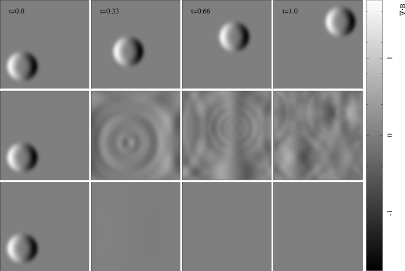
Figure 3.1: A fluid with uniform velocity has a blob of divergence introduced to the initial conditions. In the top row, no cleaning is applied and the divergence blob is advected exactly with the flow. Undamped cleaning (purely hyperbolic) is applied to the centre row and the divergence in the magnetic field is spread through the system as a system of interacting waves. In the bottom row, damped cleaning (mixed hyperbolic/parabolic) is utilised and the divergence in the magnetic field is rapidly removed.

3.4.1.1 Setup

The domain is a square area of fluid in the region $x,y\in[-0.5,1.5]$. The system has uniform density $\rho=1$, with pressure $P=6$ and $\gamma=5/3$. The velocity field is ${\bf v}=[1,1]$ and $B_{z}=1/\sqrt{4\pi}$. A perturbation is created in the x-component of the magnetic field of the form

$$B_{x}=\frac{1}{\sqrt{4\pi}}\left[\left(r/r_{0}\right)^{8}-2\left(r/r_{0}\right)^{4}+1\right];\hskip 28.45274ptr<r_{0},$$ (3.25)

where $r\equiv\sqrt{x^{2}+y^{2}}$ and $r_{0}$ specifies the radial extent. We set up the problem using $50\times 50$ particles on a square lattice, giving $h=1.2\Delta x=0.048$.

3.4.1.2 Results

Figure 3.1 shows renderings of $\nabla\cdot{\bf B}$ at various times from three calculations: no cleaning, undamped cleaning (purely hyperbolic), and damped cleaning (mixed hyperbolic/parabolic) with $r_{0}=1/\sqrt{8}$, following Dedner et al. (2002). These three calculations illustrate the basic ideas behind the divergence cleaning scheme: In the absence of any cleaning (top), the magnetic field and its divergence perturbation is advected without change on the particles. With the addition of hyperbolic cleaning (middle), the divergence errors are spread in a wave-like manner throughout the domain. Finally, the addition of the parabolic damping term (bottom row) acts to rapidly diffuse the divergence error to zero.

This is demonstrated more quantitatively in Figure 3.2, which shows the average and maximum values of $|\nabla\cdot{\bf B}|$ as a function of time for the three calculations. While purely hyperbolic cleaning can be seen to quickly reduce the maximum divergence error, the average error increases. The parabolic damping means that both the average and maximum values are reduced by an order of magnitude in roughly the time it takes for the hyperbolic waves to cross the simulation domain ($t\sim 0.3$), and by roughly 5 orders of magnitude after several crossing times ($t\gtrsim 2$). After this time the divergence error continues to decrease, but at a much slower rate (this is more obvious in Figure 3.3 for the case $r_{0}=h$). We attribute the turnover in the decay rate to the rapid removal of the short wavelength errors by the cleaning scheme, leaving only slowly decaying long-wavelength modes. This result suggests that such long-wavelength modes will decay on the order of the wave crossing time. We have confirmed this interpretation by verifying that the transition to a slow decay is independent of timestepping, resolution and is similar using the quintic (see Price, 2012) instead of the cubic spline kernel. See also Section 3.5.3.2 for further examination of this.

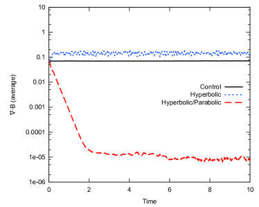
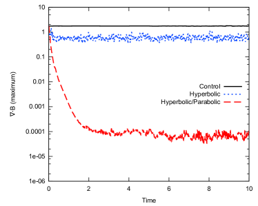
Figure 3.2: Average and maximum $\nabla\cdot{\bf B}$ in code units, measured using the difference operator (Equation 2.67), as a function of time for the divergence advection test with $r_{0}=1/\sqrt{8}$. Without cleaning, the divergence for this simple problem remains constant. Using undamped cleaning (purely hyperbolic), the maximum divergence is reduced with an increase in average throughout the system. With damped cleaning (mixed hyperbolic/parabolic), both average and maximum are rapidly reduced.

3.4.1.3 Optimal choice of damping parameter in 2D

As noted by PM05, the optimal choice of damping parameter, $\sigma_{\psi}$, for this problem with $r_{0}=1/\sqrt{8}$ is somewhat misleading, since in reality one expects divergence errors arising in simulations to have length scales of order the smoothing length. Thus, Figure 3.3 shows the average and maximum $\nabla\cdot{\bf B}$ in a series of calculations employing $r_{0}=h$ and values of $\sigma_{\psi}$ between 0.1 and 0.6. The results are similar to those shown in Figure 3.2, with best results obtained in this 2D case using $\sigma_{\psi}\sim$ 0.2–0.3.

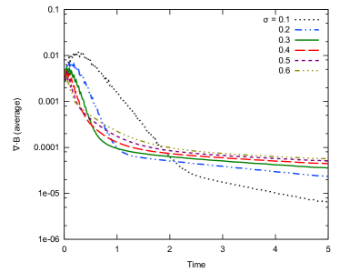
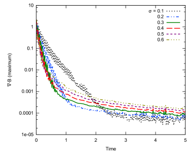
Figure 3.3: The effect of varying the damping parameter $\sigma_{\psi}$ on the average and maximum $\nabla\cdot{\bf B}$ for the divergence advection test with $r_{0}=h$. The best results for 2D are obtained for values between 0.2–0.3.

3.4.2 Static cleaning test: density jump

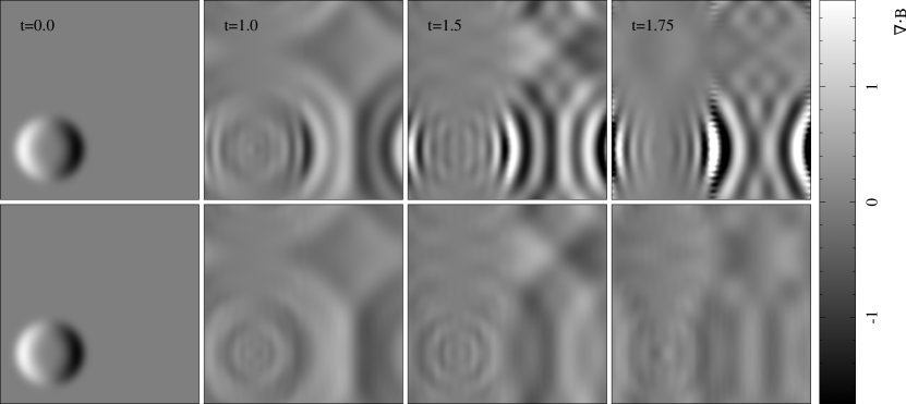
Figure 3.4: Results of the static cleaning test across a 2:1 density jump. Undamped non-conservative cleaning (top) increases the divergence of the magnetic field at the density jump, in turn leading to numerical instability (Figure 3.5). Using our constrained divergence cleaning method (bottom), the waves cross the density boundary without issue and the scheme remains stable.

Our second test is a variant on the divergence advection problem, with identical setup ($r_{0}=1/\sqrt{8}$) except that the right half of the domain has its density increased by a factor of two. The idea is to examine the reflection and refraction of the divergence waves as they transition between media of differing densities, as may frequently occur in applications of SPMHD. To simplify the test, we solve only the subset of equations given by Equations 3.1–3.2 — that is, the system can only evolve due to divergence cleaning.

3.4.2.1 Setup

The setup is performed in 2D with $25\times 50$ particles on a square lattice in the left half of the domain ($x<0.5$, $\rho=1$), and $35\times 70$ particles placed in the right half of the domain ($x>0.5$, $\rho=2$), with all particles of equal mass, giving a 2:1 density jump at $x=0.5$. The actual density on the particles is found in the usual manner by iterating the smoothing length and density self-consistently as described in Section 2.2.2. The velocity field is set to zero, all other system parameters are set as previously for the divergence advection test (Section 3.4.1), and periodic boundary conditions are employed.

3.4.2.2 Results

Figure 3.4 shows the propagation of purely hyperbolic ($\sigma_{\psi}=0$) divergence waves in this test using i) the non-energy conserving formulation with difference operators for both $\nabla\cdot{\bf B}$ (Equation 2.67) and $\nabla\psi$ (Equation 3.21), and ii) our new constrained hyperbolic divergence cleaning scheme with a difference operator for $\nabla\cdot{\bf B}$ and the conjugate, symmetric operator for $\nabla\psi$ (Equation 3.19). The corresponding time evolution of the maximum $|\nabla\cdot{\bf B}|$ is shown in Figure 3.5. Using the unconstrained formulation, the interaction of the divergence wave with the density jump causes amplification of the divergence errors (top row of Figure 3.4), in turn leading to exponential growth in the total energy and numerical instability (left panel of Figure 3.5). By contrast, our new conservative formulation remains stable and continues to reduce the divergence error throughout the domain (bottom row of Figure 3.4 and right panel of Figure 3.5).

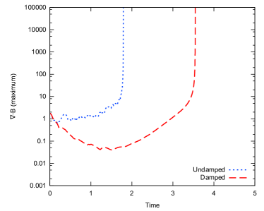
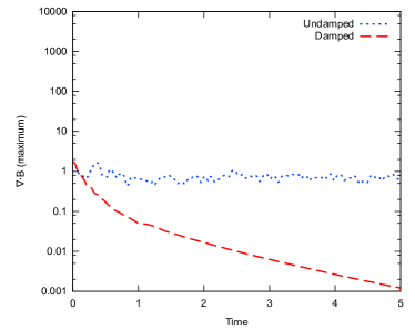
Figure 3.5: Maximum values of $\nabla\cdot{\bf B}$ (difference) for the density jump test for the non-conservative formulation (left) and the new constrained divergence cleaning (right). The interaction between the divergence waves and the density jump for the non-conservative formulation is unstable, for both damped and undamped cleaning. Using constrained divergence cleaning is stable across the density jump, with damped cleaning reducing $\nabla\cdot{\bf B}$ as in previous tests.

3.4.3 Static cleaning test: free boundaries

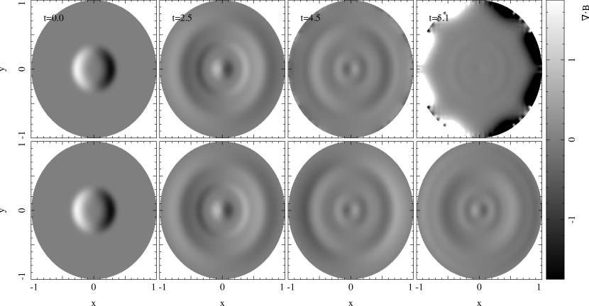
Figure 3.6: $\nabla\cdot{\bf B}$ of the static cleaning test using free boundaries. In the case of non-conservative cleaning (top row), the interaction of the divergence waves with the boundary cause unchecked divergence growth. Using constrained cleaning (bottom row), the boundary interaction is not problematic.

A further variant of the divergence advection test we consider replaces the periodic boundaries by a free boundary, since many applications of SPMHD involve free boundaries (e.g. the merger of two neutron stars, Price and Rosswog 2006, or studies of galaxy interactions, Kotarba et al. 2010, 2011).

3.4.3.1 Setup

The setup is identical to the divergence advection problem (Section 3.4.1) with $r_{0}=1/\sqrt{8}$, except that the domain is a circular area of fluid with $\rho=1$ for $r\leq 1$ and $\rho=0$ (no particles) for $r>1$, set up using a total of 1976 particles placed on a square lattice. The divergence perturbation is introduced at the centre of the circle, and the velocity field is set to zero. Rather than impose an external confining potential, we solve only Equations 3.1–3.2 without the full MHD equations, as in Section 3.4.2.

3.4.3.2 Results

Figure 3.6 shows the results of purely hyperbolic cleaning ($\sigma_{\psi}=0$) for this case. As in Figure 3.4, the top row shows the unconstrained and non-conservative difference/difference formulation, while the bottom row shows results using the conservative difference/symmetric combination. Similar results are also found in this case, with divergence errors piling up at the free boundary in the non-conservative formulation leading to numerical instability, but our constrained formulation remaining stable.

3.4.4 2D Blast wave in a magnetised medium

We now turn to tests that are more representative of the dynamics encountered in typical astrophysical simulations, beginning with a blast wave expanding in a magnetised medium. In this case the initial magnetic field is divergence-free, meaning that the only divergence errors are those created by numerical errors during the course of a simulation — rather than the artificial errors we have induced in the previous tests. Based on the results from the previous tests, in this and subsequent tests we apply cleaning only using constrained, energy-conserving formulations — that is, with conjugate operators for $\nabla\cdot{\bf B}$ and $\nabla\psi$. We use this problem to the examine the effectiveness of the divergence cleaning in the presence of strong shocks, as well as to investigate whether cleaning should be performed using the difference or symmetric $\nabla\cdot{\bf B}$ operator. As with the divergence advection test, a key goal is to find optimal values for the damping parameter $\sigma_{\psi}$.

3.4.4.1 Setup

The implementation of the blast wave follows that of Londrillo and Del Zanna (2000). The domain is a unit square with periodic boundaries, set up with $512\times 590$ particles on a triangular lattice with $\rho=1$. The fluid is at rest with magnetic field $B_{x}=10$. The pressure of the fluid is set to $P=1$, with $\gamma=1.4$, except a region of the centre of radius $0.125$ has its pressure increased by a factor of 100 by increasing its thermal energy. An adiabatic equation of state is used.

3.4.4.2 Results

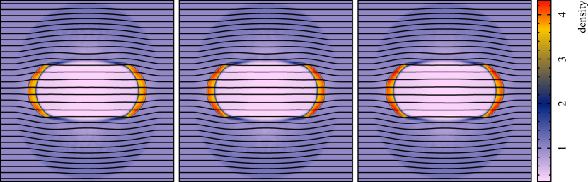
Figure 3.7: Renderings of the density together with overlaid magnetic field lines in the MHD blast wave problem at $t=0.03$, showing the control case with no resistivity and no cleaning (left), with resistivity (centre), and with divergence cleaning (right). Only minor differences in the density evolution are evident.

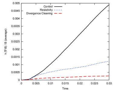
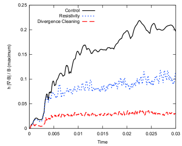
Figure 3.8: Average and maximum of $h|\nabla\cdot{\bf B}|/|{\bf B}|$ as a function of time for the blast wave test. At $t=0.03$, resistivity has reduced the average error by a factor of 4 compared to the control case, while divergence cleaning has reduced the average divergence error by a factor of 20. The maximum error has been reduced by a factor of 2 and 8, respectively.

Figure 3.7 shows the density and magnetic field lines at $t=0.03$ for i) the control case without cleaning and no artificial resistivity (left), ii) including artificial resistivity (centre) and iii) no resistivity, but cleaned using the difference operator (right). At this time, the MHD fast shock has expanded to fill the domain, yet has not crossed the periodic boundaries to begin interacting with itself, and the three cases show only minimal differences in density structure. The average and maximum divergence error as a function of time are shown in Figure 3.8. Although the density renderings at $t=0.03$ are quite similar, we can see that adding divergence cleaning has reduced the average and maximum divergence error by a factor of 20 and 8, respectively at $t=0.03$, compared to the control case, with factors of 5 and 4 improvement compared to the case with artificial resistivity alone. Thus, divergence cleaning is even more effective than resistivity at enforcing the divergence constraint.

3.4.4.3 Operator choice for $\nabla\cdot{\bf B}$

Control	Difference Cleaned	Symmetric Cleaned

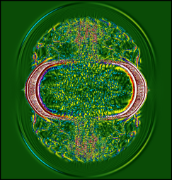
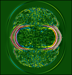
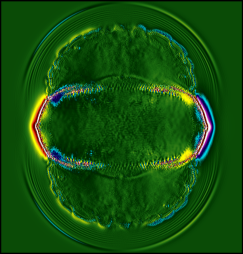
Figure 3.9: $\nabla\cdot{\bf B}$ in the blast wave problem at $t=0.03$ measured in code units using the symmetric $\nabla\cdot{\bf B}$ operator, showing the control case (left), $\nabla\cdot{\bf B}$ measured with the opposing operator to that used in the cleaning (centre) and $\nabla\cdot{\bf B}$ measured with the same operator used in the cleaning (right). Note in particular that the symmetric operator measures a divergence error around the leading edge of the fast MHD wave, even though the field is quite regular.

Control	Symmetric Cleaned	Difference Cleaned

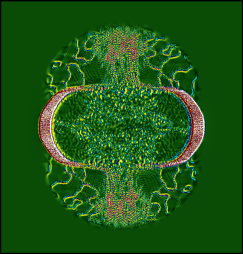
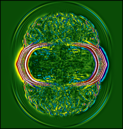
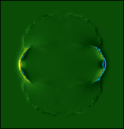
Figure 3.10: As in Figure 3.10, but showing $\nabla\cdot{\bf B}$ measured using the difference operator. With this operator, no $\nabla\cdot{\bf B}$ is measured along the leading edge of the magnetic edge for the control and difference-cleaned cases. However, symmetric cleaning produces spurious divergence in this region when measured with the difference operator, because changes have been induced in the magnetic field to compensate for particle disorder.

To answer the question of whether there is any advantage to cleaning with the symmetric $\nabla\cdot{\bf B}$ operator, the blast wave problem was simulated for three cases: no cleaning; cleaning using the difference operator for $\nabla\cdot{\bf B}$; and cleaning using the symmetric operator. The question is further complicated by fact that the operator used for cleaning may differ from the operator used to measure the error. We therefore show $\nabla\cdot{\bf B}$ for these three cases measured with both the symmetric (Figure 3.10) and difference (Figure 3.10) operators, so that the effect of cleaning using one operator can be seen in both.

The symmetric operator for $\nabla\cdot{\bf B}$ can be seen to pick up a non-zero divergence error on the leading edge of the magnetic wave from the blast (Figure 3.10) despite the fact that the magnetic field shows no error in this region when measured with the difference operator (Figure 3.10). This suggests that the symmetric operator is mainly reflecting the disordered particle arrangement. In turn, it can be seen that in this region, cleaning using the symmetric operator introduces divergence error when measured with the difference operator as it attempts to adjust the magnetic field based on the particle arrangement (centre panel of Figure 3.10). Nevertheless, it is true that cleaning with the symmetric operator does produce the greatest reduction in the divergence when measured in the symmetric operator, and may still have potential advantages in terms of momentum conservation (this is examined further in Section 3.4.5). However, we conclude that cleaning is best performed with the difference operator, since it shows not only the best results when measured with the difference operator (right panel of Figure 3.10), but also an improvement even when measured with the symmetric operator (centre panel of Figure 3.10).

3.4.4.4 Optimal damping values

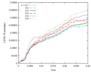
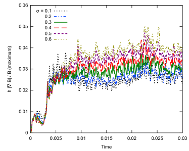
Figure 3.11: Average and maximum $h|\nabla\cdot{\bf B}|/|{\bf B}|$ for the blast wave test with varying damping strengths. The best results are obtained for values of $\sigma_{\psi}$ between 0.2–0.3.

Figure 3.11 shows the average and maximum divergence error as a function of time for differing strengths of the damping parameter $\sigma_{\psi}$ in the range $[0.1,0.6]$. The best results are obtained with $0.2<\sigma_{\psi}<0.3$, in agreement with the other two dimensional tests.

3.4.4.5 Tensile instability correction

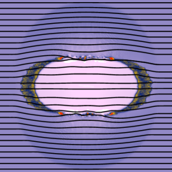
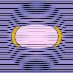
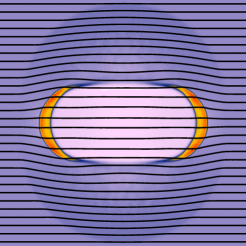
Figure 3.12: Density of the blast wave problem with overlaid magnetic field lines, without any divergence cleaning, but examining the impact of the $-\hat{\beta}{\bf B}(\nabla\cdot{\bf B})$ term used to correct the tensile instability. Results shown use $\hat{\beta}=0.5$ (left), $\hat{\beta}=0.75$ (centre) and $\hat{\beta}=1.0$ (right). Using only $\hat{\beta}=0.5$ is found to result in irregularities along the shock fronts, which are not present using $\hat{\beta}=1$. Thus, using $\hat{\beta}=0.5$ is not recommended.

Finally, we noticed important consequences in this test concerning the $\hat{\beta}{\bf B}(\nabla\cdot{\bf B})$ correction for the tensile instability (Section 2.2.8). Since using $\hat{\beta}=0.5$ is in principle sufficient to prevent the instability, its use has been suggested by Børve et al. (2004), Barnes et al. (2012), and Price (2012). However, we found this to be problematic in our simulations of the blast wave problem: Figure 3.12 shows the density with overlaid magnetic field lines at $t=0.03$ using ${\hat{\beta}}$ = 0.5, 0.75 and 1.0 (left to right). With only $\hat{\beta}=0.5$ (left panel), irregularities can be seen to form in the densest parts of the shockwave. These are not present when performing the full $\hat{\beta}=1$ subtraction (right panel).

3.4.5 Orszag-Tang Vortex

The final two dimensional test is the Orszag-Tang vortex (Orszag and Tang, 1979), which has been widely used as a test of MHD codes (e.g. Fromang et al., 2006; Stone et al., 2008; Dolag and Stasyszyn, 2009). It consists of a magnetic vortex superimposed onto a velocity vortex generating several classes of interacting shock waves. The complex dynamics provides an excellent test of the constrained hyperbolic divergence cleaning method. To measure the effectiveness of the method in this case, the results are compared against that of simulations using artificial resistivity (with particle independent strengths as described in Section 2.2.11.2) and Euler Potentials as measures of divergence control. This test is also used to examine whether or not cleaning using the symmetric operator for $\nabla\cdot{\bf B}$ provides any advantage in terms of momentum conservation. As previously, the damping parameter $\sigma_{\psi}$ is varied to find optimal values.

3.4.5.1 Setup

The problem is set up in a box with dimensions $x,y\in[0,1]$ with periodic boundary conditions. The initial gas state is set to $\rho=25/(36\pi)$, $P=5/(12\pi)$, $\gamma=5/3$, with velocity field ${\bf v}=[-\sin(2\pi y),\sin(2\pi x)]$. The initial magnetic field is ${\bf B}=[-\sin(2\pi y),\sin(4\pi x)]$. All examples presented use $512\times 590$ particles initially arranged on a triangular lattice.

3.4.5.2 Results

Control	Resistivity	Euler Potentials	Divergence Cleaning

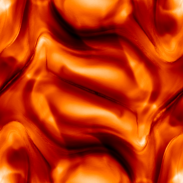
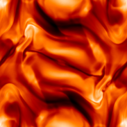
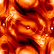
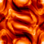
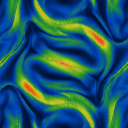
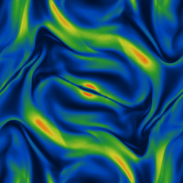
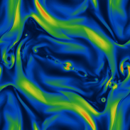
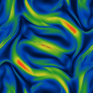
Figure 3.13: The density (top row), magnetic pressure (middle row), and the difference measurement of $\nabla\cdot{\bf B}$ (bottom row) in the Orszag-Tang vortex at $t=1.0$ comparing the control case (far left), including artificial resistivity (centre left), evolving the magnetic field using Euler Potentials (centre right), and applying the constrained divergence cleaning method (far right).

Figure 3.13 shows the density (top), magnetic pressure (middle row), and $\nabla\cdot{\bf B}$ (bottom row) at $t=1.0$ for four cases: i) control, ii) using artificial resistivity, iii) employing Euler Potentials, and iv) applying divergence cleaning. This time is chosen because the divergence errors in the control case are large enough to produce small scale disturbances in the density and magnetic pressure fields. By adding resistivity or using Euler Potentials, the average $h|\nabla\cdot{\bf B}|/|{\bf B}|$ is decreased by an order of magnitude (c.f. second and third panels in bottom row of Figure 3.13 and the left panel of Figure 3.14). When divergence cleaning is used, the average divergence error is reduced by almost two orders of magnitude (red/dashed line in left panel of Figure 3.14). In addition to the average and maximum divergence error for the above four cases, Figure 3.14 also presents the results from a case where artificial resistivity has been applied in tandem with divergence cleaning. In this case, the average $h|\nabla\cdot{\bf B}|/|{\bf B}|$ is reduced by nearly an order of magnitude compared to resistivity alone, and when compared to the control case, this results in two orders of magnitude reduction in the average together with an order of magnitude reduction in the maximum.

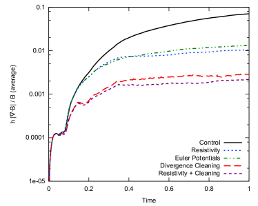
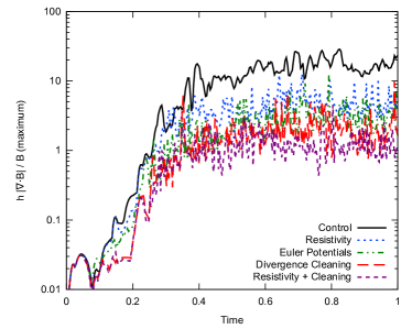
Figure 3.14: Average (left) and maximum (right) $h|\nabla\cdot{\bf B}|/|{\bf B}|$ in the Orszag-Tang vortex problem with (top to bottom in left panel) no divergence control, using Euler Potentials, adding an artificial resistivity, using divergence cleaning, and cleaning while including resistivity. Divergence cleaning has lower divergence error than when using Euler Potentials or artificial resistivity, and continues to reduce divergence error even when used in combination with artificial resistivity.

3.4.5.3 Cleaning using symmetric $\nabla\cdot{\bf B}$

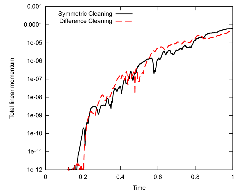
Figure 3.15: Total linear momentum for the Orszag-Tang vortex for divergence cleaning using the difference and symmetric operators of $\nabla\cdot{\bf B}$. There is no significant distinction between the two.

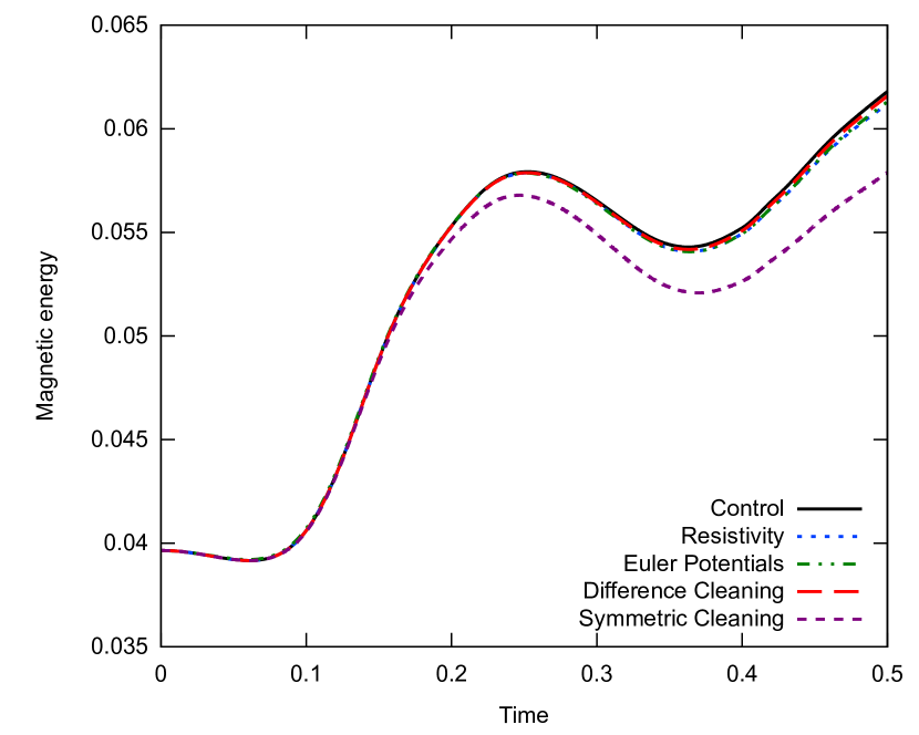
Figure 3.16: Magnetic energy as a function of time in the Orszag-Tang vortex test. Using the symmetric form of $\nabla\cdot{\bf B}$ for divergence cleaning leads to a $10\%$ reduction in magnetic energy by $t=0.5$ compared to the other schemes.

Since the symmetric operator for $\nabla\cdot{\bf B}$ is used in the momentum equation and tensile instability correction term, it was hoped that its use for cleaning would confer some advantage over the difference measure by way of improved momentum conservation. However, as shown in Figure 3.16, no significant difference in the momentum is found between cleaning with the symmetric operator compared to the difference operator. Figure 3.16 shows the magnetic energy profile of the system for $t\leq 0.5$, where all test cases (control, resistivity, Euler Potentials, difference cleaning) yield the same profile, except for symmetric cleaning which shows a $\sim 10\%$ reduction in magnetic energy compared to the other solutions. This occurs due to the symmetric operator removing magnetic energy to compensate for irregularities in particle position (which begin to occur at $t\sim 0.15$). Furthermore, although we have already shown in Section 3.4.4.3 that use of ${\hat{\beta}}=\tfrac{1}{2}$ in the tensile instability correction could result in numerical artefacts in the blast wave test, we also found large errors in the density and magnetic field profiles when ${\hat{\beta}}=\tfrac{1}{2}$ is used in combination with symmetric cleaning on the Orszag-Tang problem. For these reasons, we recommend using $\hat{\beta}=1$ and applying cleaning only with the difference $\nabla\cdot{\bf B}$ operator.

3.4.5.4 Optimal damping values

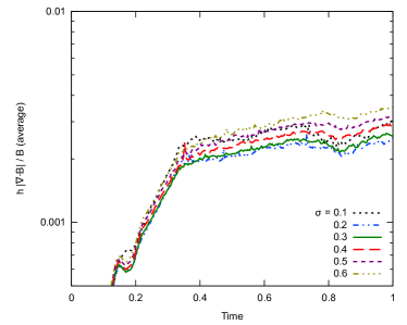
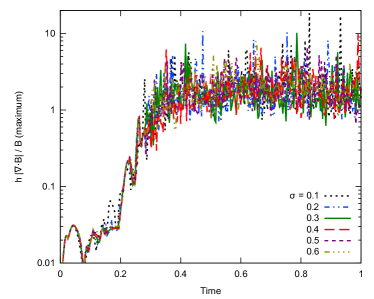
Figure 3.17: Average (left) and maximum (right) divergence error in the Orszag-Tang vortex problem, varying the damping parameter $\sigma_{\psi}$. The best results are obtained with values $\sim 0.2-0.3$.

As with the previous tests, the damping parameter $\sigma_{\psi}$ was varied to find the best results (Figure 3.17), which, as previously, were obtained for $0.2<\sigma_{\psi}<0.3$ for this 2D test.

3.4.5.5 Resolution study

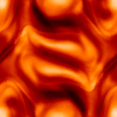
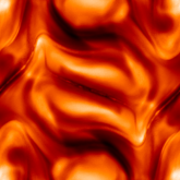
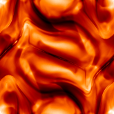
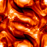
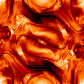
Figure 3.18: Density of the Orszag-Tang vortex at resolutions of $128\times 148$, $256\times 296$, $512\times 590$, and $1024\times 1182$ particles (left to right), with comparison to results obtained using the Athena code for $1024^{2}$ grid cells (far right). As the resolution is increased, high density islands begin to form which is also observed in results from the Athena code.

Finally, the Orszag-Tang vortex test was performed for a series of increasing resolution: $128\times 148$, $256\times 296$, $512\times 590$, and $1024\times 1182$ particles. Divergence cleaning, without resistivity, was used for all cases. The densities of these runs at $t=1.0$ are shown in Figure 3.18, along with results obtained using the Athena code (Stone et al., 2008) with $1024^{2}$ grid cells. In the largest resolution case, high density islands begin to form in the solution. These features arise from the tearing mode instability of non-ideal MHD (Furth et al., 1963), caused by magnetic reconnection along a current sheet. They are also exhibited in the results from the Athena code, and can be seen at lower resolutions in SPMHD when the Euler Potentials are used (see Figure 3.13 for an example). Despite the symmetrical initial state, the islands show artificial asymmetries resulting from momentum not being exactly conserved in SPMHD. Figure 3.19 shows the average and maximum divergence error (left and right panels, respectively). Though the maximum error remains similar for all cases, the average is seen to decrease with increasing resolution.

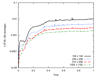
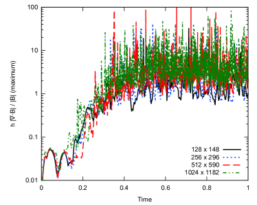
Figure 3.19: Average (left) and maximum (right) divergence error in the Orszag-Tang vortex at resolutions of $128\times 148$, $256\times 296$, $512\times 590$, and $1024\times 1182$ particles. The maximum divergence error remains similar for the different resolutions, but the average divergence error decreases with increasing resolution.

3.4.6 Three dimensional divergence advection

We now turn to 3D tests, beginning with a three dimensional generalisation of the divergence advection problem. In particular, we wish to determine the optimal values for $\sigma_{\psi}$ when the divergence waves propagate in three dimensions rather than two.

3.4.6.1 Setup

The principle of the test remains similar to 2D versions, except a cubic volume of fluid is used in the region $x,y,z\in[-0.5,1.5]$. The initial velocity field is extended to ${\bf v}=[1,1,1]$ to add drift in the $z$-direction. The magnetic field remains as previously, $B_{z}=1/\sqrt{4\pi}$, with a spherical perturbation introduced to the $x$-component of the field as given by Equation 3.25, except now using $r=\sqrt{x^{2}+y^{2}+z^{2}}$. The radial extent $r_{0}=h$ is chosen to mimic a divergence error at the resolution scale. The density and pressure remain unchanged, with $\rho=1$, $P=6$, and $\gamma=5/3$. The problem is set up on a cubic lattice with $50^{3}$ particles.

3.4.6.2 Optimal values of the damping parameter

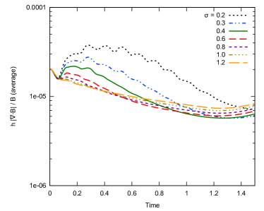
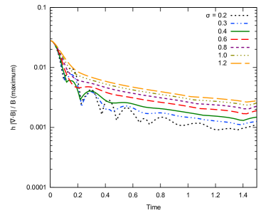
Figure 3.20: Average and maximum divergence error in the 3D advection test for varying strengths of the damping parameter, $\sigma_{\psi}$. The best results are obtained for $\sigma_{\psi}\sim$ 0.8–1.2.

This test was performed for $\sigma_{\psi}\in[0.2,1.2]$ with results of the average and maximum divergence given by Figure 3.20. The optimal cleaning is obtained for $\sigma_{\psi}\sim$ 0.8–1.2, which differs from the optimal values obtained for the 2D tests of $\sigma_{\psi}\sim$ 0.2–0.3. This is attributed to the hyperbolic wave spreading over a volume instead of an area, thus being more effective than in our 2D tests, and therefore requiring a higher value of $\sigma_{\psi}$ to achieve critical damping.

3.4.7 Gravitational collapse of a magnetised molecular cloud core

Our most complex test is drawn from our intended application: simulations of star formation that involve magnetic fields (Price et al., 2012). These simulations follow Price and Bate (2007), where an initial one solar mass sphere of gas with uniform magnetic field in the $z$-direction and in solid body rotation contracts under self-gravity to form a protostar with surrounding disc. However, at times near peak density, the magnetic field in the dense central region becomes strong and can produce high divergence errors. This has limited the range of initial magnetic field strengths which could be simulated, as if the divergence grows too large, the tensile instability correction term injects enough momentum into the system to erroneously eject the protostar out of its disc (Price and Federrath, 2010b). Thus, this simulation proves an excellent demonstration of the capabilities of the constrained hyperbolic divergence cleaning method to reduce divergence errors in realistic, 3D simulations.

3.4.7.1 Setup

This simulation uses the code, sphNG. The sphere of gas has radius $R=4\times 10^{16}\text{cm}$ with uniform density $\rho=7.43\times 10^{-18}$ g $\text{cm}^{-3}$ and is set in solid body rotation with $\Omega~{}=~{}1.77~{}\times~{}10^{-13}$ rad $\text{s}^{-1}$. A barotropic equation of state is used, as described in Price and Bate (2007). The magnetic field strength is set to give a mass-to-magnetic flux ratio of 5 times the critical value for magnetic fields to provide support against gravitational collapse. To avoid edge effects with the magnetic field, the sphere is embedded in a periodic box of length $4R$ containing material surrounding the sphere set in pressure equilibrium with density ratio 1:30. This test uses only a minimal amount of resistivity, with $\alpha_{B}\in[0,0.1]$. Self-gravity is simulated using a hierarchical binary tree where each node contains mutual nearest neighbours (Benz et al., 1990), with gravitational force softening using the SPH kernel as described by Price and Monaghan (2007). The free fall time is $\sim 24000$ years. A sink particle (Bate et al., 1995) is inserted once the gas density surpasses $\rho_{\text{sink}}=10^{-10}$ g $\text{cm}^{-3}$, and accretes particles within a radius of $6.7$ AU. The mass and momentum of accreted particles are added to the sink particle, but no information is retained about the magnetic field.

3.4.7.2 Results

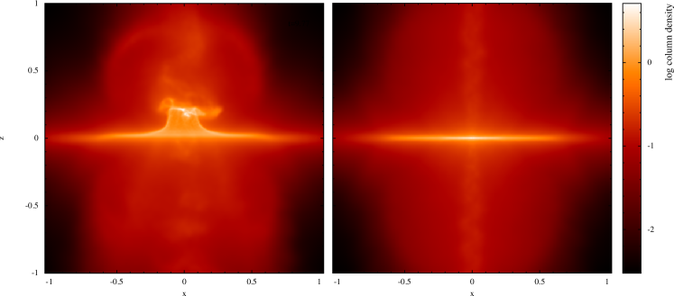
Figure 3.21: Renderings of the column density of the star formation simulation at $t=1.1$ free fall times. The simulation without cleaning (left) suffers a dramatic loss of momentum conservation (c.f. Figure 3.23) induced by high divergence errors (c.f. Figure 3.23). By contrast, the simulation with our new divergence cleaning scheme applied (right) remains stable and launches a steady, collimated outflow (Price et al., 2012).

Figure 3.21 shows column density comparisons of simulations with (right) and without (left) divergence cleaning at $t=1.1$ free fall time, showing that drastic improvements to the results are obtained by incorporating divergence cleaning. Most importantly, the protostar remains stable in its disc. The average and maximum divergence error are both reduced by roughly an order of magnitude (Figure 3.23), and this leads to a corresponding improvement in the momentum conservation of around two orders of magnitude (Figure 3.23).

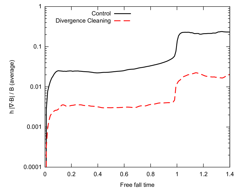
Figure 3.22: Average divergence error as a function of time for the star formation simulation, which shows that adding divergence cleaning reduces the divergence error by an order of magnitude.

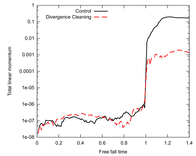
Figure 3.23: Magnitude of the total linear momentum in the star formation simulation. The system initially has zero net momentum, which increases due to the magnetic tensile instability correction and tree-based gravitational forces. After the protostar forms ($t=1$), the momentum conservation in the divergence cleaning case is improved by two orders of magnitude over the control case.

3.4.7.3 Optimal sigma values

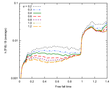
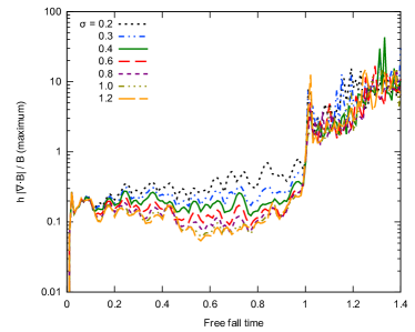
Figure 3.24: Average and maximum divergence error in the star formation simulation, varying the damping parameter in the range $\sigma_{\psi}\in[0.2,1.2]$. The best results are obtained with $\sigma_{\psi}\sim$ 0.8–1.2.

This simulation was repeated for several values of the damping parameter in the range $\sigma_{\psi}\in[0.2-1.2]$, with the results on average and maximum divergence error presented in Figure 3.24. Optimal results were obtained for $\sigma_{\psi}\sim$ 0.8–1.2, which agrees with values found for the 3D advection test (Section 3.4.6.2).

3.4.7.4 Inclusion of the $\tfrac{1}{2}\psi(\nabla\cdot{\bf v})$ term

Adding $\tfrac{1}{2}\psi(\nabla\cdot{\bf v})$ to the evolution equation for $\psi$ was motivated by energy conservation considerations, but the resulting question is what effect this has on divergence cleaning. The star formation simulation represents the ideal test case with which to examine this, with a large $\nabla\cdot{\bf v}$ present due to the gravitational collapse of the gas. We have performed this simulation both with and without this term, using $\sigma_{\psi}=0.8$, and found no distinguishable difference in the linear momentum, and average and maximum $h|\nabla\cdot{\bf B}|/|{\bf B}|$ profiles. Similar results were obtained also found in the other tests. We conclude that, although this term is necessary for strict energy conservation, it has almost zero effect on the effectiveness of the cleaning scheme.

3.4.8 Magnetised Mach 10 turbulence

To fully investigate the importance of the $\tfrac{1}{2}\psi(\nabla\cdot{\bf v})$ term, we turn to ‘turbulence in a box’ simulations of driven, magnetised, Mach 10 turbulence. Such a calculation will have many interacting shocks, and for this calculation, produces density variations up to $1000\times$ the initial density. There is substantial and continual compression and rarefaction of the gas, and as such, is the perfect testbed to test the effect of a term which includes $\nabla\cdot{\bf v}$. This test utilises the same simulation setup as in Section 4.2.6, with the full details and a comparison of results between SPMHD and grid-based methods presented in Chapter 5.

3.4.8.1 Setup

The system is set in a periodic box of unit length, $L=1$. The initial density is uniform $\rho=1$, and the initial velocity is ${\bf v}=0$. The initial magnetic field is set $B_{z}=\sqrt{2}\times 10^{-5}$. The equation of state is isothermal, $P=c_{\rm s}\rho$, with $c_{\rm s}=1$. The resolution is $128^{3}$ particles. The Morris and Monaghan (1997) switch for artificial viscosity has been used, along with the artificial resistivity switch developed in Chapter 4.

The turbulence is stochastically driven at large scales ($1<k<3$, peaked at $k=2$) by a force obtained from the Ornsetin-Uhlenbeck process (Eswaran and Pope, 1988; Federrath et al., 2010). This keeps the turbulence in a statistical steady state at rms velocity Mach 10 ($\mathcal{M}=10$). The autocorrelation time of the driving motion is one turbulent turnover time, $t_{\rm c}=L/(2\mathcal{M}c_{\rm s})$. The turbulence is driven using using only the solenoidal component of the driving force, obtained through construction in Fourier space.

The calculations have been run both with and without the $\tfrac{1}{2}\psi(\nabla\cdot{\bf v})$ term in the divergence cleaning. Both calculations use $\sigma_{\psi}=1.0$.

3.4.8.2 Results

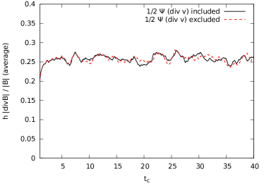
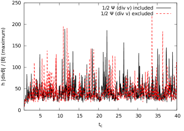
Figure 3.25: Average and maximum divergence error in the magnetised, Mach 10 turbulence calculation with and without the $\tfrac{1}{2}\psi(\nabla\cdot{\bf v})$ term in the $\psi$ evolution equation. No distinguishable difference is present between the calculations, and we conclude that this term is not important for the effectiveness of the cleaning method.

Figure 3.25 shows the average and maximum $h|\nabla\cdot{\bf B}|/|{\bf B}|$ over a period of 40$t_{\rm c}$. No distinguishable difference is found in the average and maximum divergence error. As with the star formation calculation, we conclude that the inclusion of this term does not improve the effectiveness of the cleaning and is not needed for stability. Even in the presence of strong compression and rarefaction of the gas, this term has no practical effect on the cleaning method.

3.5 Enhancing the cleaning method

The constrained implementation of mixed hyperbolic/parabolic divergence cleaning only approximately upholds the divergence-free constraint on the magnetic field. The maximum effectiveness of the cleaning is limited by the explicit timestep constraint, as it must obey the Courant condition in order to ensure stability of the hyperbolic waves. In the following section, we investigate two approaches to enhance the effectiveness of the cleaning method, in particular demonstrating how the method can be used to achieve $\nabla\cdot{\bf B}=0$.

3.5.1 Over-cleaning

The simplest approach to improve the effectiveness of the cleaning is to increase $c_{\rm h}$. Introducing a factor, $f_{\rm ovc}\geq 1$, the cleaning wave speed is adjusted to $c_{\rm h}\to f_{\rm ovc}c_{\rm h}$. This requires a corresponding reduction in timestep according to $\Delta t\to\Delta t/f_{\rm ovc}$. We call this method ‘over-cleaning’.

This incurs a significant computational cost as the full simulation is slowed down by a commensurate amount to the over-cleaning factor. If 10 times over-cleaning is used, then the simulation will run 10 times slower. This sacrifices the cheap computational cost of hyperbolic divergence cleaning, however the simplicity of this approach has found practical use by Bate et al. (2014b) who used 30$\times$ over-cleaning to reduce divergence errors in their simulations of protostar formation.

3.5.2 Sub-cycling

The second approach investigated is to cycle the cleaning equations in-between timesteps. After each timestep, the errors introduced into the magnetic field are removed by running the cleaning equations in isolation. The dynamics of the simulation halted during the sub-cycles. This is similar to the ‘static cleaning’ tests in Section 3.4.2 and 3.4.3.

This approach is significantly cheaper in computational expense compared to over-cleaning. It does not slow the evolution of the system down (timestep size remains as normal). Since the particle positions remain static during the sub-cycles, only one neighbour search is required to be performed at the start of the iterations.

A second advantage is that sub-cycling allows for the continual cleaning of the magnetic field until the error falls below a desired tolerance. This guarantees the divergence error to be below that tolerance at all times.

Implementing sub-cycling with individual timesteps requires special consideration. Consider the situation of a subset of particles which are ‘active’, surrounded by particles which are ‘inactive’. If sub-cycling is run on just the active set of particles, then the magnetic field near the boundary between the two sets of particles may be become distorted as the cleaning is unable to remove the errors on the adjacent inactive particles. Running sub-cycling on the full system is expensive (especially if the active regions constitute only a tiny fraction of the full system). One approach would be to perform iterations in a hierarchy according to the timestep bins. The particles on the smallest timestep bin could be cleaned every iteration, the particles on the second smallest timestep bin are cleaned every second iteration, and so on.

3.5.3 Numerical tests

Our tests compare the effectiveness of over-cleaning and sub-cycling. To allow direct comparison, sub-cycling is run for a fixed number of iterations so that it compares more directly to over-cleaning. However, tests are also performed where sub-cycling is run with a tolerance on the average $h|\nabla\cdot{\bf B}|/|{\bf B}|$. Following these tests, we consider a ‘static’ test of an evolved state of the Orszag-Tang vortex where the optimal value of $\sigma_{\psi}$ in the damping term for sub-cycling is investigated. We will show that sub-cycling is able to clean the magnetic field all the way to $\nabla\cdot{\bf B}=0$.

3.5.3.1 Orszag-Tang vortex

The effectiveness of over-cleaning and sub-cycling is investigated using the Orszag-Tang vortex. The initial state of the problem is described in Section 3.4.5. For these tests, we used $512^{2}$ particles arranged on a square lattice. In all cases, artificial resistivity is applied using the new resistivity switch described in Chapter 4.

The vortex is simulated using 10, 20, and 100$\times$ over-cleaning ($f_{\rm ovc}=10$, $20$, and $100$) and sub-cycling with 10, 20, and 100 iterations ($9$, $19$, and $99$ between timesteps plus the cleaning performed on the system timestep). These are intended to provide an overall level of cleaning that is comparable between the two approaches. A calculation using ‘normal’ hyperbolic divergence cleaning (with $\sigma_{\psi}=0.3$) is included to act as a reference.

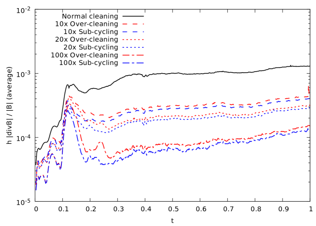
Figure 3.26: The Orszag-Tang vortex with $10$, $20$, and $100\times$ over-cleaning and $10$, $20$, and $100$ iterations of sub-cycling. Over-cleaning and sub-cycling have similar results when the over-clean factor and iteration count are the same. Each factor of 10 increase in the over-cleaning factor and sub-cycling iteration count yield half an order of magnitude reduction in average divergence error.

Figure 3.26 shows the average divergence error in the system, showing that over-cleaning and sub-cycling yield similar average divergence error when the over-cleaning factor and number of sub-cycling iterations are equal. Each factor of 10 increase in the over-cleaning factor and iteration count yield approximately half an order of magnitude decrease in average divergence error.

Table 3.1: Computational Cost of Over-cleaning and Sub-cycling

Calculation	cpu hours	Relative expense
Normal cleaning	17.6	1.0$\times$
10$\times$ over-cleaning	212.5	$12.1\times$
20$\times$ over-cleaning	460.3	$26.2\times$
100$\times$ over-cleaning	1956.0	$111.1\times$
10$\times$ sub-cycling	60.0	$3.4\times$
20$\times$ sub-cycling	96.5	$5.5\times$
100$\times$ sub-cycling	372.3	$21.2\times$
0.1% tolerance sub-cycling	25.3	$1.4\times$
0.05% tolerance sub-cycling	34.7	$2.0\times$
0.02% tolerance sub-cycling	125.1	$7.1\times$

The computational expense of the over-cleaning and sub-cycling calculations is given in Table 3.1. Over-cleaning is almost directly proportional to the over-cleaning factor used, with $10\times$ over-cleaning corresponding to $12\times$ increase in computation time. On the other hand, 10 iterations of sub-cycling only increases computation time by $3.4\times$. Overall, sub-cycling is ${\sim}~{}4$–$5$ times more computationally efficient than over-cleaning.

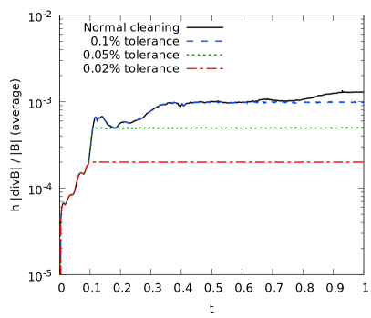
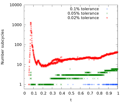
Figure 3.27: The average divergence error in the Orszag-Tang vortex when sub-cycling is used to keep the average error below $0.1\%$, $0.05\%$, and $0.02\%$. The right panel shows the number of iterations required per timestep. The large peak in the $0.02\%$ tolerance case at $t~{}{\sim}~{}0.15$ is due to the particles breaking off their initial lattice arrangement, requiring ${\sim}~{}1000$ iterations for this case to treat.

Additional simulations were performed where sub-cycling was run until the average divergence error was below $0.1\%$, $0.05\%$, and $0.02\%$. There was no limit placed on the number of iterations. Figure 3.27 shows the average divergence error is maintained at the specified tolerance.

The number of iterations per sub-cycle step is given in the second panel of Figure 3.27. The $0.1\%$ average error case requires no iterations until late in the simulation, and then only an extra 1 or 2 per timestep. The $0.05\%$ average error case is under 10 iterations at all time. However, the $0.02\%$ average error case requires ${\sim}1000$ iterations early when the particles first break off their initial lattice arrangement ($t~{}{\sim}~{}0.15$), after which $20$–$40$ iterations are performed on average. A simulation was performed where the tolerance on average divergence error was set to $0.01\%$, but this caused a prohibitive number of iterations at $t~{}{\sim}~{}0.15$ ($>10^{5}$ iterations). It would be advisable to impose a maximum number of iterations to prevent such situations from stalling the calculation.

We note that no high density islands form in any of the over-cleaning or sub-cycling calculations. These features appeared in the $512\times 590$ particle calculation using Euler Potentials (Figure 3.13), as well as the high resolution $1024\times 1182$ particle divergence cleaning calculation from Figure 3.18 and the Athena calculation in the same figure. They do not appear in the $2048^{2}$ particle calculations performed in Section 4.2.5, despite being even higher resolution. The difference in the $2048^{2}$ particle calculations is they included an artificial resistivity, whereas the $1024\times 1182$ particle calculation did not. The formation of these features is related to the tearing mode instability of non-deal MHD (Furth et al., 1963), whereby magnetic reconnection causes magnetic islands to form along current sheets. Thus, these features are related to the dissipation of the magnetic field, not from divergence errors in the magnetic field, though are sensitive to the degree of resistivity present. For example, they form in the $1024\times 1182$ particle calculation when no artificial resistivity is applied, yet do not form in the higher resolution $2048^{2}$ calculation when a minimal amount of artificial resistivity is present. They form in the $512\times 590$ particle Euler Potentials calculation, yet do not appear in the over-cleaning and sub-cycling calculations of similar resolution (but which contain artificial resistivity).

3.5.3.2 Static test: cleaning to $\nabla\cdot{\bf B}=0$

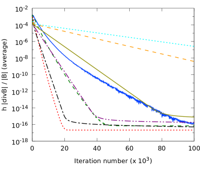
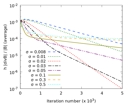
Figure 3.28: Comparing values of $\sigma_{\psi}$ in the damping parameter to obtain an optimal value for sub-cycling, with the left panel for $10^{5}$ iterations and right panel the first $5000$. Short wavelength errors are quickly removed using $\sigma_{\psi}=0.3$ (right panel), though performs poorly at removing slowly long wavelength modes (left panel). Using $\sigma_{\psi}=0.03$, though initially worse at reducing divergence error, is found to remove long wavelength errors in the shortest number of iterations.

The tolerance on average divergence error may be set arbitrarily low when performing sub-cycling, and it is possible to achieve $\nabla\cdot{\bf B}=0$ as we will show.

For this test, we take the $t~{}=~{}1$ evolved state of the Orszag-Tang vortex from the reference calculation in Section 3.5.3.1, and perform sub-cycling for $10^{5}$ iterations. Figure 3.28 shows the average divergence error versus iteration count for a set of calculations varying the $\sigma_{\psi}$ parameter in the damping term. Our results show that $\nabla\cdot{\bf B}=0$ is achievable to arbitrarily small precision in SPMHD, provided a sufficient number of iterations are performed.

The calculations requiring the minimum number of iterations to reach average divergence error below $10^{-15}$ are the $\sigma_{\psi}=0.02$–$0.03$ cases (${\sim}~{}10^{4}$ iterations). These $\sigma_{\psi}$ values are $10\times$ smaller than the optimal value of $\sigma_{\psi}$ found during the testing of the divergence cleaning method ($0.03$ to $0.3$). The $\sigma_{\psi}~{}=~{}0.3$ case still has not reached $<10^{-15}$ average divergence error after $10^{5}$ iterations. This difference may be understood through the differing rates on the removal of small and long wavelength errors. The right panel of Figure 3.28 shows the first 5000 iterations of these set of calculations, which shows that $\sigma_{\psi}~{}\sim~{}0.3$ provides the most rapid reduction of divergence error for the first ${\sim}~{}300$ iterations. Divergence error is introduced into the system at small wavelengths, which this level of damping is most effective at removing (and hence is optimal when the system is evolving and continually injecting divergence error). However, the reduction of average divergence error slows significantly after ${\sim}~{}300$ iterations because at that stage, only large wavelength errors remain which slowly decay. While $\sigma_{\psi}~{}{\sim}~{}0.03$ is initially worse, the hyperbolic waves are allowed to propagate more effectively, averaging the errors throughout the system, which in turn allows the diffusion term to become more effective at reducing the long wavelength modes.

To investigate this further, we performed a calculation using a static snapshot of the Orszag-Tang vortex where cleaning was performed each iteration using a range of damping values between $\sigma_{\psi}\in[0.01,0.4]$, with the value of $\sigma_{\psi}$ that yielded the largest reduction in divergence error being accepted and the magnetic field evolved one step with that value. This process was repeated each timestep, with the aim of mapping out the optimal values of $\sigma_{\psi}$ for high numbers of iterations. It was found that the $\sigma_{\psi}$ oscillated each iteration below the maximum value (0.4) and the minimum value (0.01) for ${\sim}~{}500$ iterations, then remained at $\sigma_{\psi}=0.01$ for ${\sim}~{}500$ iterations, with this pattern repeating. It initially yielded reduction of divergence error on par with the fixed $\sigma_{\psi}=0.3$ case, with long-term reduction similar, but not as rapid, as the fixed $\sigma_{\psi}=0.03$ case. Considering these results, it would be best to run sub-cycling with fixed $\sigma_{\psi}=0.3$ for several hundred iterations to remove short wavelength errors, then switch to $\sigma_{\psi}=0.03$ for the reduction of long wavelength errors.

We also make note that the choice of time integration scheme is important when taking $>10^{3}$–$10^{4}$ iterations. The errors introduced from Euler integration can become significant over this many iterations, corrupting the magnetic field. Leapfrog integration may be implemented with a predictor step for $\psi$ (as it depends upon both itself and ${\bf B}$) in a manner similar to Section 2.2.12. It does require derivative evaluations of $\nabla\psi$ (for ${\rm d}{\bf B}/{\rm d}t$) and $\nabla\cdot{\bf B}$ (for ${\rm d}\psi/{\rm d}t$) to occur out of phase with each other. The tests performed here use a second order Runge-Kutta scheme, which we find to be adequate.

3.6 Velocity divergence cleaning for weakly compressible SPH

Incompressible fluids are divergence-free in the velocity field, thus approaches utilised to satisfy the magnetic divergence constraint can be adapted to work with the velocity divergence constraint. A popular method is incompressible SPH (ISPH), which uses a projection method to construct a divergence-free velocity field via the solution of a Poisson equation (Cummins and Rudman, 1999). Another is weakly compressible SPH (WCSPH), where, rather than directly ensure the velocity field is divergence-free, a stiff equation of state is used to limit density variations. Both have advantages and disadvantages, as highlighted in the comparison of Lee et al. (2008). In short, WCSPH is simple to program, but ISPH tends to produce smoother velocity and pressure fields. ISPH has the computational expense of solving an elliptic equation, but WCSPH is also expensive because its high sound speed produces small timesteps due to the Courant condition. ISPH is known to produce numerical instability if particle distributions become highly disordered, though there have been attempts to modify ISPH to fix this issue (Shao and Lo, 2003; Hu and Adams, 2007; Lind et al., 2012). Xu et al. (2009) tested and compared a number of ISPH approaches.

In this section, the constrained hyperbolic divergence cleaning method is adapted for use on the velocity field, and test its effectiveness at reducing density variations in the weakly compressible approximation (see also Tricco and Price, 2012b).

3.6.1 Weakly compressible SPH

A common method for modelling incompressible fluid behaviour with SPH is to use a stiff equation of state with the standard Lagrangian SPH formulation. This sacrifices true incompressibility for simplicity of implementation. However, this does not imply computational efficiency as the high speed of sound ($\sim 10\times$ maximum fluid velocity as a minimum) necessitates small sized time steps for stability. Using the equation of state

$$P=\frac{c_{\rm s}^{2}\rho_{0}}{7}\left(\left(\frac{\rho}{\rho_{0}}\right)^{7}-1\right),$$ (3.26)

where $\rho_{0}$ is the reference density of the fluid and $c_{\rm s}$ is the sound speed, this typically results in density variations of $\sim 1\%$ (Monaghan, 1994).

The equations of motion which are solved are

$$\frac{{\rm d}{\bf v}_{a}}{{\rm d}t}=-\sum_{b}m_{b}\left(\frac{P_{a}}{\rho_{a}^{2}}+\frac{P_{b}}{\rho_{b}^{2}}\right)\nabla_{a}W_{ab}.$$ (3.27)

In this case, we evolve the density using the SPH equivalent of the continuity equation (Equation 2.41) rather than by summation, as this can lead to sharper profiles near free surfaces. The smoothing length of the particles is held constant, initially calculated according to Equation 2.43.

3.6.2 Hyperbolic divergence cleaning for the velocity field

Since the continuity equation relies on $\nabla\cdot{\bf v}$ to evolve density, minimising this quantity should lead to improvements in the representation of incompressibility. We now construct a formulation of divergence cleaning suitable for the velocity field. The cleaning equations to be solved are modified to become

$$\frac{{\rm d}{\bf v}}{{\rm d}t}= -\frac{\nabla\psi}{\rho},$$ (3.28)

$$\frac{{\rm d}\psi}{{\rm d}t}= -c_{\rm h}^{2}\rho\nabla\cdot{\bf v}-\frac{\psi}{\tau}.$$ (3.29)

As the intended application is for incompressible fluids, we assume throughout this section that the density is uniform and constant. Equations 3.28 and 3.29 still combine to produce the equivalent of the damped wave equation of Equation 3.3.

We follow a procedure in step with that of Section 3.2. Consider the closed system of equations given by Equations 3.28 & 3.29. The total energy of this velocity-cleaning subsystem is

$$E=\int\left[\frac{v^{2}}{2}+\tilde{e}_{\psi}\right]\rho{\rm d}V,$$ (3.30)

where $\tilde{e}_{\psi}$ is the energy of the $\psi$ field. Constraining the energy of this subsystem to be conserved implies

$$\frac{{\rm d}E}{{\rm d}t}=\int\left[{\bf v}\cdot\frac{{\rm d}{\bf v}}{{\rm d}t}+\chi\frac{{\rm d}\psi}{{\rm d}t}\right]\rho{\rm d}V=0,$$ (3.31)

where $\chi$ is an unspecified variable to be determined. Inserting Equation 3.28 and 3.29 yields

$$\int\left[-{\bf v}\cdot\frac{\nabla\psi}{\rho}-\chi c_{\rm h}^{2}\rho\nabla\cdot{\bf v}\right]\rho{\rm d}V=0.$$ (3.32)

Integrating the first term by parts, we obtain

$$\int\left[\frac{\psi}{\rho}-\chi c_{\rm h}^{2}\rho\right](\nabla\cdot{\bf v})\rho{\rm d}V+\int_{s}\psi{\bf v}\cdot{\rm d}\hat{s}=0,$$ (3.33)

which leads to $\chi=\psi/c_{\rm h}^{2}\rho^{2}$ and hence

$$\tilde{e}_{\psi}=\frac{\psi^{2}}{2c_{\rm h}^{2}\rho^{2}}.$$ (3.34)

Using this energy term in Equation 3.30 will yield ${\rm d}\rho/{\rm d}t$ terms, but we neglect the addition of these terms under the assumption of incompressibility.

3.6.3 Discretised hyperbolic velocity divergence cleaning

With the appropriate energy term for this cleaning system, the constrained SPH implementation may be constructed. We clean using the same $\nabla\cdot{\bf v}$ operator as in the continuity equation, that is,

$$\nabla\cdot{\bf v}_{a}=-\frac{1}{\rho_{a}}\sum_{b}m_{b}{\bf v}_{ab}\cdot\nabla_{a}W_{ab}.$$ (3.35)

The SPH discretised version of Equation 3.30 is

$$E=\sum_{a}m_{a}\left[\frac{v_{a}^{2}}{2}+\frac{\psi_{a}^{2}}{2c_{\rm h}^{2}\rho_{a}^{2}}\right].$$ (3.36)

Differentiating with respect to time and using Equations 3.29 and 3.35, we obtain

$$\sum_{a}m_{a}{\bf v}_{a}\frac{{\rm d}{\bf v}_{a}}{{\rm d}t}=\sum_{a}\frac{m_{a}\psi_{a}}{\rho_{a}^{2}}\sum_{b}m_{b}{\bf v}_{ab}\cdot\nabla_{a}W_{ab}.$$ (3.37)

By splitting the RHS into two halves, swapping summations on one half, then combining, it is concluded that

$$\frac{{\rm d}{\bf v}_{a}}{{\rm d}t}=-\sum_{b}m_{b}\left(\frac{\psi_{a}}{\rho_{a}^{2}}+\frac{\psi_{b}}{\rho_{b}^{2}}\right)\nabla_{a}W_{ab}.$$ (3.38)

As before, conjugate operators for $\nabla\cdot{\bf v}$ and $\nabla\psi$ become imposed. In addition to exactly conserving energy, this form for $\nabla\psi$ also conserves momentum. The evolution equation for $\psi$ is

$$\frac{{\rm d}\psi_{a}}{{\rm d}t}=c_{\rm h}^{2}\sum_{b}m_{b}{\bf v}_{ab}\cdot\nabla_{a}W_{ab}-\frac{\psi}{\tau}.$$ (3.39)

3.6.4 Oscillating water drop test

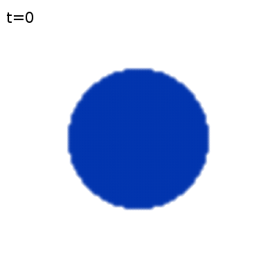
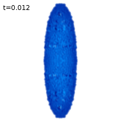
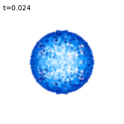
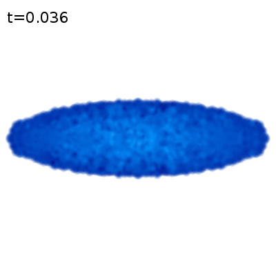
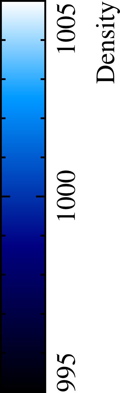
Figure 3.29: Snapshots of the oscillating water drop test. The circular drop has an initial velocity which squeezes it into an elliptical shape along the $y$-axis. A radial force is present which halts the expansion of the drop, then contracts it to its original shape before expanding along the opposite axis. This behaviour repeats causing the drop to oscillate alternately along the two axes.

To investigate the effectiveness of our velocity cleaning algorithm, it is applied to an oscillating elliptic water drop. The water drop is initially circular and is free standing. A radial force is exerted upon it, and with an initial velocity which is compressional along one axis, the drop oscillates, squeezing alternately along the two axes. This behaviour is demonstrated in Figure 3.29.

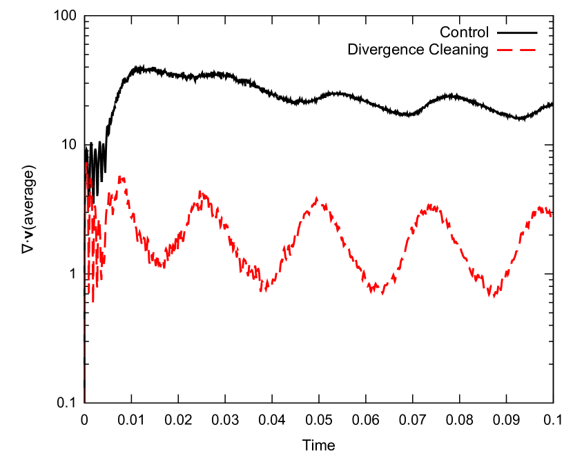
Figure 3.30: Average $\nabla\cdot{\bf v}$ of the elliptic water drop test. Average velocity divergence is reduced by approximately an order of magnitude when divergence cleaning is applied.

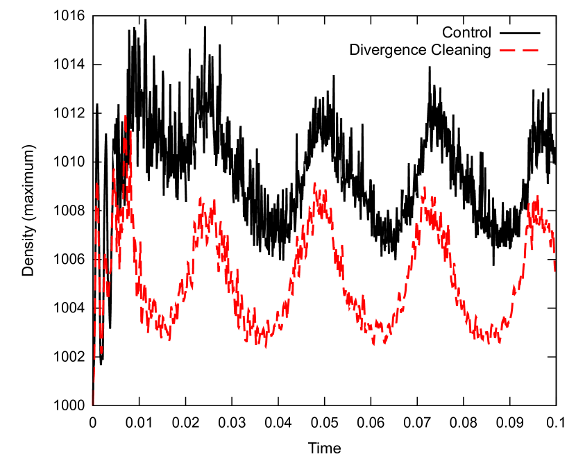
Figure 3.31: Maximum density variation during the elliptic water drop test. Applying divergence cleaning to the velocity field reduces density changes from the reference density by $\sim 0.5$.

The drop is modelled using the weakly compressible approximation (Equations 3.27 and 2.41 with Equation 3.26 as the equation of state). The reference density is $\rho_{0}=1000$ kg $\text{m}^{-2}$, and the initial velocity field is ${\bf v}=[-100x,100y]$. The radial force is $-100^{2}{\bf r}$. The drop has radius $R=1$, and a total of $1976$ particles are used arranged on a square lattice.

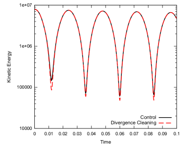
Figure 3.32: Total kinetic energy of the elliptic water drop test. No significant discrepancies exist between the control and divergence cleaned tests.

The evolution of the drop is tracked until $t=0.1$, approximately two oscillation periods. Figure 3.31 shows the average velocity divergence of the system as a function of time for both the cleaned and uncleaned systems. Applying cleaning reduces the average divergence by nearly an order of magnitude, similar to results obtained for magnetic field cleaning. This leads to a reduction in maximum density error by a factor of two (Figure 3.31). The dissipation of kinetic energy by the cleaning algorithm is insignificant, as shown in Figure 3.32.

3.7 Summary

In this chapter we have developed an implementation of Dedner et al. (2002)’s hyperbolic divergence cleaning for SPMHD that is constrained to be numerically stable and to always decrease the magnetic energy (see also Tricco and Price, 2012a). To achieve this, we first defined the energy associated with the scalar $\psi$ field (Section 3.2.2). This term was used to show that when the density varies over time, the evolution equation of $\psi$ should be modified to include a $-\tfrac{1}{2}\psi(\nabla\cdot{\bf v})$ term in order to conserve energy.

In Section 3.3.2 we derived an energy conserving formulation of divergence cleaning for SPMHD. By using the $\psi$ energy term, we showed that if a difference operator is chosen to discretise $\nabla\cdot{\bf B}$ in the ${\rm d}\psi/{\rm d}t$ equation, then the conjugate, symmetric operator for $\nabla\psi$ should be used (Section 3.3.2.1). Similarly, with symmetric $\nabla\cdot{\bf B}$, difference $\nabla\psi$ should be used in the induction equation (Section 3.3.2.2). Use of conjugate operators was found to be the key to a numerically stable formulation. In Section 3.3.2.3, we presented the correct SPMHD form of the $-\tfrac{1}{2}\psi(\nabla\cdot{\bf v})$ term, and in Section 3.3.3, demonstrated that parabolic damping will always lead to negative definite changes of energy.

Tests of our constrained hyperbolic divergence cleaning were presented in Section 3.4. The selection of tests were for both 2 and 3D, and were designed to evaluate our method in isolation using simple, idealised systems and also in more realistic applications. Our idealised 2D tests consisted of a divergence advection test (Section 3.4.1), and variants involving a density jump (Section 3.4.2) and free boundaries (Section 3.4.3). The more complex 2D tests were an MHD blast wave (Section 3.4.4) and the Orszag-Tang vortex (Section 3.4.5). A version of the divergence advection test extended to 3D was used in Section 3.4.6. Results from the gravitational collapse of a molecular cloud core, representing our most challenging test case and a gauge of divergence cleaning applied to “real” applications, were presented in Section 3.4.7. Calculations of magnetised, supersonic turbulence were examined in Section 3.4.8. From the results of these tests, we draw the following conclusions:

1. Constrained hyperbolic/parabolic divergence cleaning provides an effective method of maintaining the divergence constraint in SPMHD, typically maintaining the average $h|\nabla\cdot{\bf B}|/|{\bf B}|$ to between 0.1–1%.

2. The constrained formulation using conjugate operators for $\nabla\cdot{\bf B}$ and $\nabla\psi$ is stable at density jumps and free boundaries, in contrast to previous implementations.

3. We strongly recommend cleaning using the difference operator for $\nabla\cdot{\bf B}$. Cleaning using the symmetric operator was not found to provide any advantage over the difference operator in terms of momentum conservation and was found to dissipate physical components of the magnetic field as well as the divergence error.

4. Constrained divergence cleaning is more effective than artificial resistivity at reducing the divergence error, and still reduces the divergence error further when used in combination with resistivity.

5. Divergence cleaning can provide an improvement of up to two orders of magnitude in momentum conservation when applied to realistic, 3D simulations.

6. Optimal values for the damping parameter $\sigma_{\psi}$ were found to be $\sigma_{\psi}=$ 0.2–0.3 in 2D and $\sigma_{\psi}=$ 0.8–1.2 in 3D for all of the test problems considered in this thesis.

7. Addition of the $-\tfrac{1}{2}\psi\nabla\cdot{\bf v}$ term to the ${\rm d}\psi/{\rm d}t$ equation, while necessary for strict energy conservation of the hyperbolic cleaning equations, was found to have no noticeable effect even when the gas is strongly compacted, such as in simulations of star formation and magnetised, Mach 10 turbulence.

8. We found numerical artefacts in several problems when subtracting only $-\tfrac{1}{2}{\bf B}(\nabla\cdot{\bf B})$ in the momentum equation to counteract the tensile instability. Instead, we strongly recommend using the full $-{\bf B}(\nabla\cdot{\bf B})$ correction.

Two approaches were investigated to enhance the cleaning method in Section 3.5: Over-cleaning, where the cleaning wave speed is explicitly increased with a corresponding decrease in the size of the timestep, and sub-cycling, where the cleaning equations are solved in isolation between timesteps. Both reduce the average divergence error, yielding half an order of magnitude reduction per factor of ten increase in wave speed or number of sub-cycle iterations. Sub-cycling is able to keep average divergence error below a specified tolerance at all times, and it was shown that given enough iterations, the divergence error may be reduced to arbitrarily low limits. It was found that high number of iterations ($>300$), using $\sigma_{\psi}=0.03$ is optimal to reduce long wavelength errors.

In Section 3.6, we constructed cleaning equations for the velocity field for use in weakly compressible SPH simulations (see also Tricco and Price, 2012b). The velocity divergence cleaning equations conserve energy and momentum. When the velocity field was cleaned in weakly compressible SPH simulations of an oscillating water drop, density variations were reduced by half, with negligible kinetic energy dissipation. Though these results are encouraging, additional work is required, in particular, for cases involving boundary particles.

In summary, our constrained hyperbolic divergence cleaning scheme is a robust and effective method for enforcing the divergence constraint in SPMHD simulations, providing a pathway to accurate simulation of a wide range of magnetic phenomena in astrophysics and beyond.

Declaration for Chapter 4

Declaration by Candidate

In the case of Chapter 4, the nature and extent of my contribution to the work was the following:

Nature of Contribution	Extent of Contribution (%)
First author of 2013, “A switch to reduce resistivity in smoothed particle magnetohydrodynamics”, MNRAS 436, 2810–2817.	90

The following co-authors contributed to the work:

Name	Nature of Contribution	Extent of Contribution (%) for student co-authors
Daniel Price	PhD supervisor

The undersigned hereby certify that the above declaration reflects the nature and extent of the candidate’s and co-author’s contributions to this work.

Chapter 4 A switch to reduce resistivity

Magnetised shocks and discontinuities pervade the interstellar medium (Elmegreen and Scalo, 2004; Gaensler et al., 2011). Capturing these properly in numerical simulations is critical to accurately predicting the formation of stars from turbulent, magnetised, molecular clouds (Federrath and Klessen, 2012), and this necessitates adding numerical dissipation to simulations. On the other hand, estimates of the microscopic viscosity and resistivity in the interstellar medium suggest very high values of the kinematic and magnetic Reynolds numbers, respectively, typically orders of magnitude higher than can be achieved in numerical codes (c.f. Elmegreen and Scalo, 2004). Thus, it is important to minimise numerical dissipation in simulation codes. This is typically done by improving the shock capturing scheme so that dissipation away from shocks is reduced, though the Reynolds number near the shock may still be decreased.

The usual approach to shock-capturing in SPH is to treat discontinuities in fluid variables by adding dissipation terms which smooth the variable across sharp jumps in order to resolve the discontinuity (Section 2.2.10). Artificial viscosity for treatment of hydrodynamic shocks was developed by Monaghan and Gingold (1983). In this work, we use the form of artificial viscosity by Monaghan (1997), developed by analogy with Riemann solvers (Section 2.2.10.1). In SPMHD, an artificial resistivity for the magnetic field is included to capture magnetic shocks and discontinuities (i.e., current sheets) (Section 2.2.10.2). However, the choice of signal velocity in the artificial resistivity is less clear than for the artificial viscosity. Ideal MHD has three wave solutions but without reconstructing the full Riemann state it is not possible to determine the type of shock. Thus, this is typically chosen to be the speed of the fast MHD wave. Since this is rather dissipative, Price (2012) instead suggested using the averaged Alfvén velocity as the choice of signal velocity (though see Section 4.2.6)

A switch may be employed for $\alpha_{\text{B}}$ to reduce dissipation away from shocks. Price and Monaghan (2005) (PM05) suggested a switch based on analogy with Morris and Monaghan (1997) (see Section 2.2.11.2). This switch works satisfactorily for many problems, leading to sharper jump profiles and a decrease in the overall dissipation of the magnetic field. However, Price et al. (2012) noted in their star formation simulations that, even with this switch, excess dissipation could suppress the formation of protostellar jets.

Our need for a new resistivity switch is motivated by the failure of the PM05 switch in the limit where the Alfvén speed is much smaller than the sound speed, as will be shown in section 4.2.6. Since $\alpha_{\text{B}}\propto|\nabla\times{\bf B}|$ (assuming $\nabla\cdot{\bf B}$ is negligible), this means that $\alpha_{\text{B}}$ is related to the magnitude of the magnetic field. Thus, for weak fields $\alpha_{\text{B}}$ may remain quite small even in the presence of strong shocks.

In this chapter, we present a new switch for $\alpha_{\text{B}}$ that captures shocks in the magnetic field in both weak and strong fields. This addresses the deficiencies of the previous switch and results in less overall dissipation of magnetic energy. The chapter is organised as follows: In Section 4.1, the new resistivity formulation and implementation is described. Section 4.2 contains a suite of tests designed to test the efficacy of the new switch and to compare results against the previous switch. Section 4.3 extends the concept of the switch to develop switches for artificial viscosity and thermal conductivity. Results are summarised in Section 4.4.

4.1 Formulation

Our approach is to utilise $\nabla{\bf B}$, the $3\times 3$ gradient matrix of ${\bf B}$, as the shock indicator. For each particle, $\alpha_{\text{B}}$ is directly set to the dimensionless quantity

$$\alpha_{\text{B},a}=\frac{h_{a}|\nabla{\bf B}_{a}|}{|{\bf B}_{a}|}.$$ (4.1)

This is artificially restricted to the range $\alpha_{\rm B}\in[0,1]$ so that zero dissipation is applied in regions away from discontinuities.

By using the norm of the gradient of the magnetic field normalised by the magnitude of the magnetic field, the dependence on magnetic field strength is removed and this gives a relative measure of the strength of the discontinuity. This allows shocks and discontinuities to be robustly detected in both the weak and strong field regimes. It naturally produces values of $\alpha_{\text{B}}$ in the desired range and of the appropriate size for the discontinuity encountered, with regions away from shocks having negligible $\alpha_{\text{B}}$ values.

The numerical dissipation of the magnetic field in regions away from shocks should scale quadratically with resolution when using this switch. Consider a magnetic field which has a linear gradient, that is $\nabla{\bf B}$ is constant and resolution independent. It is clear then that the switch is proportional to the resolution length, that is, for example, $\alpha_{\rm B}$ will decrease by half when the resolution is doubled ($h$ is halved). Since artificial resistivity itself scales linearly with resolution, as is evident from Equation 2.95, it is clear that using Equation 4.1 will yield artificial resistivity that scales quadratically.

The switch produces the same $\alpha_{\text{B}}$ values for multiplicative increases in magnetic field strength, important for dynamo-type problems where the magnetic field grows in strength. This represents a significant advantage over the PM05 switch. Additive increases to the magnetic field, however, will yield different values of $\alpha_{\text{B}}$, and using this switch in relativistic contexts would require further consideration.

An obvious issue is what happens when $|{\bf B}|\to 0$. This situation occurs in current sheets or null points where the magnetic field undergoes a reversal in direction. In these cases, $\alpha_{\text{B}}\to 1$, which is the correct behaviour for current sheets since they represent a discontinuity in the magnetic field, but is not so for null points. Dividing by zero can be avoided by adding a small parameter $\epsilon$ to $|{\bf B}|$.

4.1.1 Implementation

Each component of the gradient matrix is estimated using a standard SPH first derivative operator (e.g., Equation 2.58),

$$\nabla{\bf B}_{a}\equiv\frac{\partial B^{i}_{a}}{\partial x^{j}_{a}}=-\frac{1}{\Omega_{a}\rho_{a}}\sum_{b}m_{b}({B}^{i}_{a}-{B}^{i}_{b})\nabla_{a}^{j}W_{ab}(h_{a}).$$ (4.2)

This operator yields an estimate which is exact for constant functions. We also investigated using an operator that is exact for linear functions, which may be obtained by performing a Taylor series expansion about ${\bf r}_{a}$ and solving a matrix inversion of the second error term (see Section 2.2.3). However, no difference was found for any of the tests shown in this thesis, suggesting that this is unnecessary.

The norm of $\nabla{\bf B}$ is calculated using the 2-norm,

$$|\nabla{\bf B}|\equiv\sqrt{\sum_{i}\sum_{j}\left|\frac{\partial B^{i}_{a}}{\partial x^{j}_{a}}\right|^{2}}.$$ (4.3)

Several choices for computing this norm were investigated, such as the 1-norm, but no significant differences were found.

We investigated using the curl of the magnetic field as the shock indicator. While tests found it to be just as effective at detecting isolated shocks, we found that it did not measure discontinuities as well as the full gradient in complicated shock interactions. The full gradient has further advantage in that the trace of the matrix produces the divergence of the field, meaning that dissipation will be applied if large divergence errors are present.

Finally, a Cullen and Dehnen (2010)-like approach was also investigated, whereby a time-dependent decay term for $\alpha_{\text{B}}$ was added, similar to that in other artificial viscosity switches (Section 2.2.11.1) and the PM05 switch. In this case, $\alpha_{\text{B}}$ was set using Equation 4.1 whenever this exceeded the current value, otherwise the existing value was retained and subsequently reduced on the next integration timestep using the decay term. The aim was to let $\alpha_{\text{B}}$ smoothly decay after a shock had passed to improve representation of the post-shock field. We found that using Equation 4.1 alone already gives a smooth distribution in $\alpha_{\text{B}}$ about the centre of the shock, indicating that a decay term is not necessary for resistivity.

4.1.2 Choice of signal velocity

Similar to Price (2012) we take the signal velocity to be an average of the wave speeds between the two particles

$$v^{B}_{\text{sig}}=0.5(v_{{\rm mhd},a}+v_{{\rm mhd},b}),$$ (4.4)

where $v_{\rm mhd}$ is an appropriate MHD wave speed. The $-\beta{\bf v}_{ab}\cdot\hat{{\bf r}}_{ab}$ term used in the viscosity signal velocity, which corrects for the relative velocity of the particles and prevents particle interpenetration, is not included. We find that for resistivity it is unnecessary and causes excessive dissipation. It may be noted that use of the averaged Alfvén speed for a signal velocity by Price (2012) also excluded this term.

Unlike Price (2012), we find that the best choice is to use the fast MHD wave speed, as in the original Price and Monaghan (2004a) formulation, such that

$$v_{\rm mhd}^{2}=\frac{1}{2}\left(c^{2}_{{\rm s},a}+v_{{\rm A},a}^{2}\right)+\frac{1}{2}\sqrt{(c_{{\rm s},a}^{2}+v_{{\rm A},a}^{2})^{2}-4c_{{\rm s},a}^{2}v_{{\rm A},a}^{2}(\hat{{\bf B}_{a}}\cdot\hat{{\bf r}}_{ab})},$$ (4.5)

which is a composition of the sound speed, $c_{\rm s}$, and the Alfvén speed, $v_{\rm A}=B/\sqrt{\mu_{0}\rho}$. See Section 2.1.4 for more information on MHD waves. If $c_{\rm s}\gg v_{\rm A}$, we find that Price (2012)’s suggestion to use the Alfvén speed in the applied resistivity is insufficient to capture fast wave shocks (see Section 4.2.6). When $v_{\rm A}\gtrsim c_{\rm s}$, the Alfvén speed and the fast wave speed will differ by less than a factor of 2.

4.1.3 Switches using a second derivative

In principle, a switch constructed using a higher derivative should provide a more reliable measure of the presence of a discontinuity in the magnetic field. One suggestion by Walter Dehnen (priv. commun.) is to use $\alpha_{\text{B}}=h|\nabla^{2}{\bf B}|/|\nabla{\bf B}|$. Another option could be $\alpha_{\text{B}}=h^{2}|\nabla^{2}{\bf B}|/|{\bf B}|$, which would scale quadratically with resolution.

The main difficulty in implementing higher derivative switches is calculating the second derivative in a way which is sufficiently free of noise from particle disorder. We investigated calculating $\nabla^{2}{\bf B}$ using the Brookshaw (1985) form, that is,

$$\nabla^{2}{\bf B}_{a}=\frac{2}{\Omega_{a}\rho_{a}}\sum_{b}m_{b}\left({\bf B}_{a}-{\bf B}_{b}\right)\frac{F_{ab}(h_{a})}{|r_{ab}|},$$ (4.6)

where $\nabla W_{ab}\equiv\hat{\bf r}_{ab}F_{ab}$, and also by taking two first derivatives as in Equation 4.2, which, by taking two successive first derivatives, should lead to a more smooth estimate of the second derivative. However, both of these simple estimates are significantly noisy when the particles are disordered, leading to high $\alpha_{\text{B}}$ and excessive dissipation. The M6 quintic spline kernel was used in an attempt to reduce this noise, both by yielding a more regular particle distribution and a more accurate derivative estimate, but did not change the results.

Therefore, a switch utilising the second derivative must use a higher order estimate in order to reduce noise from particle disorder, a conclusion similarly reached by Cullen and Dehnen (2010) and Read and Hayfield (2012). The most straightforward approach is to use two exact linear first derivatives which removes the $O(h)$ error term by taking a Taylor series expansion about ${\bf r}_{a}$ and performing a matrix inversion of the second error term. Specifically, after first calculating $\nabla{\bf B}$ in such a manner, we compute

$$\chi^{\sigma\gamma}\frac{\partial{\nabla{\bf B}}^{\alpha\beta}_{a}}{\partial{\bf x}^{\sigma}}=\sum_{b}m_{b}\left[(\nabla{\bf B})_{b}^{\alpha\beta}-(\nabla{\bf B})_{a}^{\alpha\beta}\right]\nabla^{\gamma}W_{ab}$$ (4.7)

to obtain $\nabla^{2}{\bf B}$, where $\chi^{\sigma\gamma}=\sum_{b}m_{b}({\bf r}_{b}-{\bf r}_{a})^{\sigma}\nabla^{\gamma}W_{ab}$ is the $3\times 3$ matrix that must be inverted (see Equations 2.59 and 2.60). This significantly improves the quality of the second derivative estimate, but requires two loops over the particles prior to the main loop where the resistivity term is calculated, meaning that it makes the overall SPMHD scheme $\sim 1.5\times$ more expensive. This is a hefty price to pay for a switch that only marginally improves over Equation 4.1. The second derivative evaluation proposed by Read and Hayfield (2012) is even more expensive, requiring a $10\times 10$ matrix inversion, and a minimum of 400 neighbours under the kernel.

Our overall conclusion is to prefer the simple switch of Equation 4.1 for general use. It performs robustly and effectively (see Section 4.2), yet is simple to implement and cost-effective.

4.2 Numerical Tests

Our choice of tests are designed to study the ability of the switch to i) properly capture and model shock phenomena, and ii) suppress dissipation in areas away from shocks. We have used three shocktube tests to study the former, using tests introduced by Dai and Woodward (1994) and Brio and Wu (1988) (corresponding to tests 1B, 2A, and 5A in Ryu and Jones (1995) (hereafter RJ95) whose naming convention we adopt). These tests contain fast and slow shocks, fast and slow rarefactions, rotational discontinuities, and compound shock structures and are chosen to test the switch’s ability to model all these separate shock types. We then compare the new switch to the PM05 switch for three separate test problems: Propagation of a circularly polarised Alfvén wave, the Orszag-Tang vortex, and Mach 10 shocks in a fluid with an extremely weak field. The last test is of particular interest because, as will be shown, the PM05 switch fails to recognise shocks in this weak field regime causing unphysical behaviour.

All our tests employ the constrained divergence cleaning algorithm of Chapter 3. The tests presented here serve to further validate this scheme.

4.2.1 Shocktube 1B

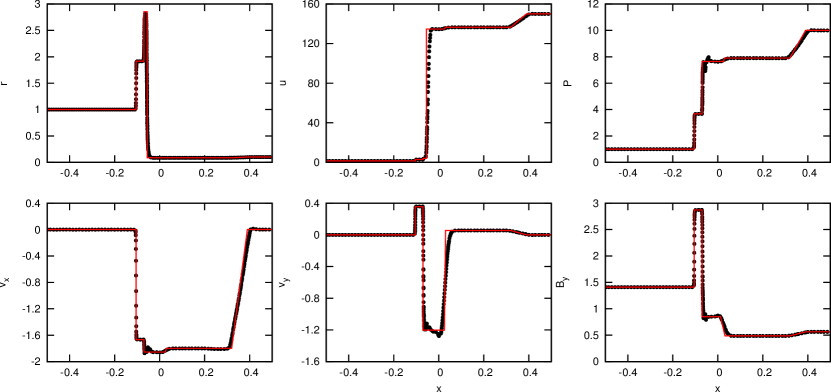
Figure 4.1: Shocktube test 1B from RJ95 performed in 2D with left state ($\rho$, $P$, $v_{x}$, $v_{y}$, $B_{y}$) $=$ (1, 1, 0, 0, $5/\sqrt{4\pi}$) and right state ($\rho$, P, $v_{x}$, $v_{y}$, $B_{y}$) $=$ (0.1, 10, 0, 0, $2/\sqrt{4\pi}$) with $B_{x}=3/\sqrt{4\pi}$ at $t=0.03$. Black circles are the particles and the red line is the solution from RJ95.

The first shocktube is a 2D test from Dai and Woodward (1994) which creates fast and slow shocks travelling in the -x direction, fast and slow rarefactions travelling in the +x direction, with a contact discontinuity in the centre. The initial state for $x<0$ (the ‘left state’) is ($\rho$, $P$, $v_{x}$, $v_{y}$, $B_{y}$) $=$ (1, 1, 0, 0, $5/\sqrt{4\pi}$), while for $x>0$ (the ‘right state’) is ($\rho$, P, $v_{x}$, $v_{y}$, $B_{y}$) $=$ (0.1, 10, 0, 0, $2/\sqrt{4\pi}$) with $B_{x}=3/\sqrt{4\pi}$ and $\gamma=5/3$.

For this particular test, the initial density profile was used to calculate the initial thermal energy so that it forms a smooth transition between the two states. This mitigates the presence of artificial pressure spikes in the initial conditions due to the high density contrast ($10$:$1$), seen also by Hubber et al. (2013) in their studies of Kelvin-Helmholtz instabilities.

The shocktube has been simulated with 800$\times$26 particles for the left state and 260$\times$8 particles for the right state arranged on a triangular lattice. Artificial viscosity has been applied with a constant $\alpha=1$, as has been for subsequent shocktube tests. Results at $t=0.03$ are shown in Figure 4.1 and may be compared with the RJ95 solution for the fast and slow shock and rarefactions (red line). The L1 error in the $B_{y}$ profile is $8.911\times 10^{-3}$. This compares to $9.547\times 10^{-3}$ if the shocktube is run using the PM05 switch.

For this shocktube test, it is worth noting that no difficulties were found with our divergence cleaning algorithm. Recently, Stasyszyn et al. (2013) published a different implementation and found that for this test it resulted in significant errors unless the cleaning was artificially limited. Their method is equivalent to using the PM05 implementation (that is, difference operators for both $\nabla\cdot{\bf B}$ and $\nabla\psi$), but with an artificial limiter that restricts corrections to the magnetic field to remain less than local changes due to the induction equation. As we have demonstrated in Sections 3.4.2–3.4.3, the PM05 implementation is numerically unstable and causes amplification of divergence error at sharp density contrasts. For the sharp $10:1$ density ratio in this shocktube, the artificial limiter used by Stasyszyn et al. (2013) inhibits the instability from corrupting the magnetic field at the interface. Our method instead inherently fixes the numerical stability, without the need for artificial limiters, by formulating the cleaning equations so that they manifestly conserve energy (see Chapter 3).

4.2.2 Shocktube 2A

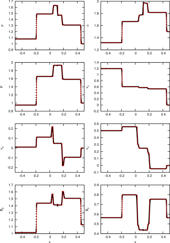
Figure 4.2: Shocktube test 2A from RJ95 performed in 3D with left state ($\rho$, $P$, $v_{x}$, $v_{y}$, $v_{z}$, $B_{y}$) $=$ (1.08, 0.95, 1.2, 0.01, 0.5, $3.6/\sqrt{4\pi}$) and right state ($\rho$, P, $v_{x}$, $v_{y}$, $v_{z}$, $B_{y}$) $=$ (1, 1, 0, 0, 0, $4/\sqrt{4\pi}$) with $B_{x}=B_{z}=2/\sqrt{4\pi}$ at $t=0.2$. Black circles are the particles and the red line is the solution from RJ95.

This 3D problem originally introduced by Dai and Woodward (1994) has three dimensional velocity and magnetic fields generating two fast and slow shocks travelling in both directions, two rotational discontinuities, and a contact discontinuity in the centre. It has left state ($\rho$, $P$, $v_{x}$, $v_{y}$, $v_{z}$, $B_{y}$) $=$ (1.08, 0.95, 1.2, 0.01, 0.5, $3.6/\sqrt{4\pi}$) and right state ($\rho$, P, $v_{x}$, $v_{y}$, $v_{z}$, $B_{y}$) $=$ (1, 1, 0, 0, 0, $4/\sqrt{4\pi}$) with $B_{x}=B_{z}=2/\sqrt{4\pi}$ and $\gamma=5/3$.

To fully capture the 3D velocity and magnetic fields, the test has been simulated in 3D with 800$\times$12$\times$12 particles on the left state and 500$\times$12$\times$12 particles on the right state arranged on close-packed triangular lattices. Results at $t=0.2$ are presented in Figure 4.2 with all shock features, with the red line giving the solution from RJ95. No post-shock noise in the magnetic field is evident, indicating that the applied artificial resistivity is sufficient. The L1 error in the $B_{y}$ profile is $3.086\times 10^{-3}$, compared to $3.358\times 10^{-3}$ if the PM05 switch is used instead, and for the $B_{z}$ profile is $5.33\times 10^{-3}$ for our new switch and $6.203\times 10^{-3}$ for the PM05 switch.

4.2.3 Shocktube 5A

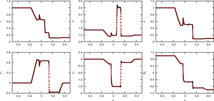
Figure 4.3: Shocktube test 5A from RJ95 performed in 2D with left state ($\rho$, $P$, $v_{x}$, $v_{y}$, $B_{y}$) $=$ (1, 1, 0, 0, 1) and right state ($\rho$, P, $v_{x}$, $v_{y}$, $B_{y}$) $=$ (0.125, 0.1, 0, 0, -1) with $B_{x}=0.75$ at $t=0.1$. Black circles are the particles and the red line is the solution obtained with the Athena code using $10^{4}$ grid cells.

The final shocktube originates from Brio and Wu (1988). It is another 2D shocktube, however it is of particular interest as it contains a compound shock/rarefaction structure. It has the same initial density and pressure profile as the standard Sod shocktube (Sod, 1978), but with the addition of a magnetic field. The left state is ($\rho$, $P$, $v_{x}$, $v_{y}$, $B_{y}$) $=$ (1, 1, 0, 0, 1) and right state ($\rho$, P, $v_{x}$, $v_{y}$, $B_{y}$) $=$ (0.125, 0.1, 0, 0, -1) with $B_{x}=0.75$. Here we use $\gamma=5/3$ instead of $2$ to follow the results of RJ95.

The shock has been simulated with 800$\times$30 particles for the right state and 300$\times$10 particles for the right state. Results at $t=0.1$ are presented in Figure 4.3. For this test, the Riemann solution of RJ95 does not contain the slow compound structure, so instead we compare our results against those from the Athena code (Stone et al., 2008) using $10^{4}$ grid cells. As previously, no post-shock noise in the magnetic field is found. The L1 error profile for $B_{y}$ is $4.231\times 10^{-3}$ when using our new switch, compared to $6.259\times 10^{-3}$ if the PM05 switch is used.

4.2.4 Polarised Alfvén Wave

We now examine the ability of the switch to reduce dissipation when no shocks are present. The test problem used is a circularly polarised Alfvén wave travelling in a 2D periodic box, following Tóth (2000). This is an exact solution to the ideal MHD equations, so the wave should return to its original state after each crossing. There are no discontinuities in the magnetic field in this test, but gradients in the magnetic field may cause the $\alpha_{\text{B}}$ switch to activate.

The simulation is set up using $1682$ particles arranged on a triangular lattice in a periodic domain of lengths $[x,y]=[1/\cos(\omega),1/\sin(\omega)]$ using $\omega=\pi/6$ which sets the direction of wave motion. The initial density and pressure are $\rho=1$ and $P=0.1$ with $\gamma=5/3$. The velocity and magnetic fields parallel and perpendicular to the wave are $[v_{\parallel},v_{\perp}]=[0,0.1\sin(2\pi x_{\xi})]$, and $[B_{\parallel},B_{\perp}]=[1,0.1\sin(2\pi x_{\xi})]$ where $x_{\xi}=x\cos(\omega)+y\sin(\omega)$. Velocity and magnetic field components oriented out of the plane are $v_{z}=B_{z}=0.1\cos(2\pi x_{\xi})$. Artificial viscosity is not applied in this test in order to minimise dissipation of energy in the system.

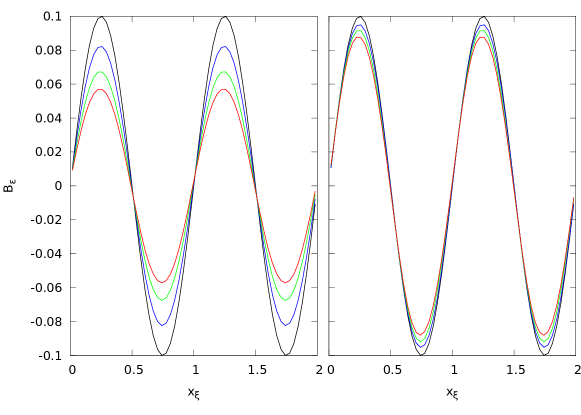
Figure 4.4: Results of the polarised Alfvén wave propagation test in 2D, with the exact solution in black, and at $t=2,4,6$ corresponding to 2, 4, and 6 periods. On the left, the PM05 switch has been used whereas on the right the new resistivity switch has been used. The maximum $\alpha_{\text{B}}$ values are $10\times$ higher for the PM05 switch than the new switch, and after 6 periods the amplitude of the wave has decayed over $40\%$ for the PM05 switch compared to only $10\%$ for the new switch.

The value of $\alpha_{\text{B}}$ produced using the new switch can be calculated from the initial conditions, which give $|\nabla{\bf B}|=0.2\pi$ and $|{\bf B}|=1$. Thus, for a smoothing length $h=1.2\Delta x$ where $\Delta x$ is the particle spacing, the new switch gives $\alpha_{\text{B}}\sim 0.02$ at this resolution. By contrast, the simulations using the PM05 switch produce maximum $\alpha_{\text{B}}$ values approximately $10\times$ higher ($0.22$ vs $0.02$), meaning that in this case the PM05 switch is an order of magnitude more dissipative at $t=0$.

After 6 periods, the amplitude of the wave has decayed by over $40\%$ using the PM05 compared to only $\sim 10\%$ for the new switch. Although the maximum $\alpha_{\text{B}}$ is $10\times$ higher with the PM05 switch than the new switch, this is not reflected in the wave amplitude after 6 periods because $|\nabla{\bf B}|$ and the source term in the PM05 switch (Equation 2.106) are reduced as the wave is damped. The rate of this reduction differs between the two switches since the PM05 switch damps the wave more heavily.

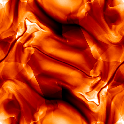
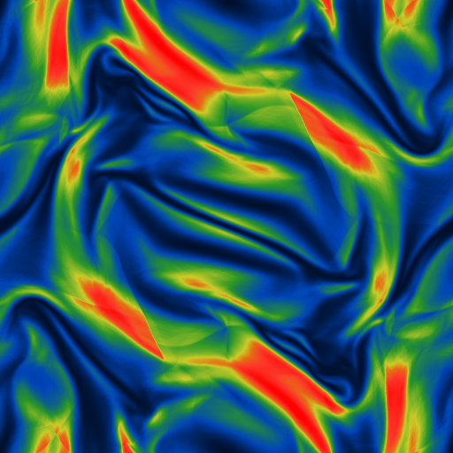
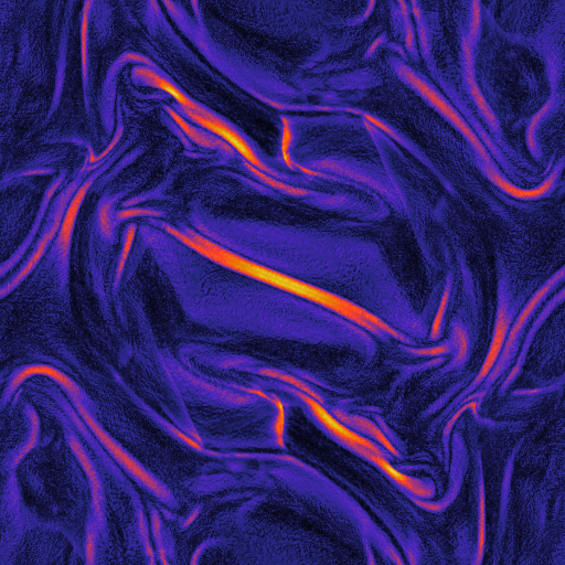
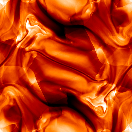
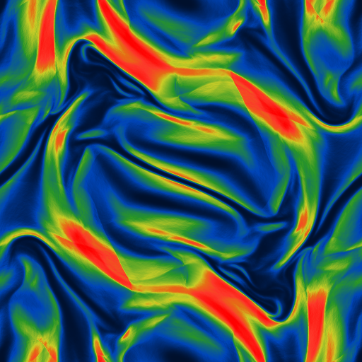
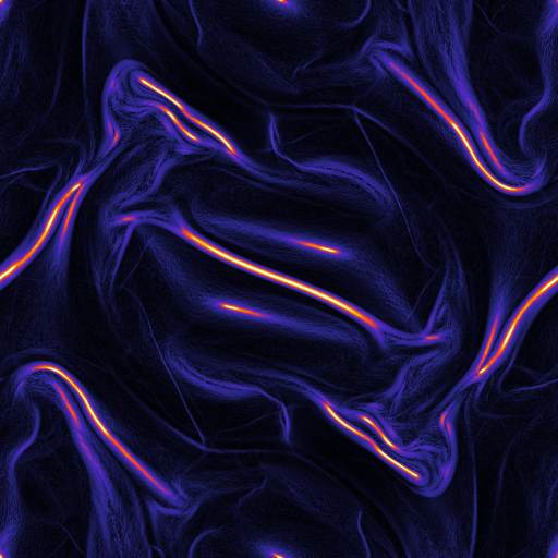
Figure 4.5: The density, magnetic pressure, and $\alpha_{\text{B}}$ (left to right panels) of the Orszag-Tang vortex at $t=1$ for the old (top row) and new (bottom row) resistivity switches. The new switch effectively traces the shock lines, with little or no dissipation between shocks. The low density regions are more sharply defined using the new switch due to the decreased dissipation of the magnetic field structure.

4.2.5 Orszag-Tang vortex

The Orszag-Tang vortex (Orszag and Tang, 1979) is a widely used test for many astrophysical MHD codes (e.g., Fromang et al., 2006; Stone et al., 2008; Dolag and Stasyszyn, 2009). The problem has an initial vortex structure creating several classes of interacting shock waves which evolve into turbulence, with the initial conditions as given in Section 3.4.5.

The test has been simulated using $512^{2}$, $1024^{2}$, and $2048^{2}$ particles initially arranged on a square lattice. The initial conditions are set up by first creating the particles in one quadrant of the domain, then mirroring the configuration to the other quadrants with appropriate sign changes in the velocity and magnetic fields as needed. This removes the slight discrepancies from floating point arithmetic, retaining exact symmetry in the initial conditions. The Morris and Monaghan (1997) switch for artificial viscosity has been used.

Results are presented at $t=1$ in Figure 4.5 which shows renderings of the density, magnetic pressure, and $\alpha_{\text{B}}$ in the domain for $1024^{2}$ particles. The new switch is effective at activating resistivity along the shock lines, yet keeps $\alpha_{\text{B}}$ minimal between shocks. By contrast, the PM05 switch results in broad regions with $\alpha_{\text{B}}\approx 1$ near shocks and a mean $\alpha_{\text{B}}$ twice as high ($\sim 0.2$ to $\sim 0.1$). This leads to a smoothing away of subtle magnetic features, particularly noticeable around the central magnetic feature, and in some of the low density regions which are less sharply defined.

Figure 4.6 shows the evolution of the magnetic energy as a function of time for $512^{2}$, $1024^{2}$, and $2048^{2}$ particles. This shows that the magnetic energy is dissipated less at higher resolution. Using the new artificial resistivity switch also leads to a lower dissipation rate compared to the PM05 switch, producing an effect equivalent to running the test at higher resolution.

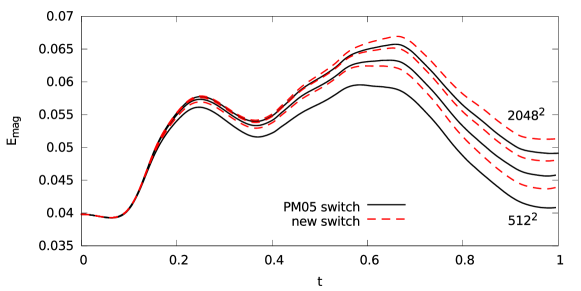
Figure 4.6: Evolution of the magnetic energy for the Orszag-Tang vortex using the PM05 resistivity switch (black, solid lines) and the new resistivity switch (red, dashed lines) at resolutions of $512^{2}$, $1024^{2}$, and $2048^{2}$ particles. The new switch is much less dissipative than the PM05 switch, producing an effect similar to increasing the resolution.

4.2.6 Mach 10 MHD turbulence

Our final test is of supersonic magnetised turbulence which is representative of conditions in molecular clouds (see reviews by Evans, 1999; Elmegreen and Scalo, 2004; McKee and Ostriker, 2007). A stochastic, solenoidal driving force is applied, generating turbulence with a root-mean-square Mach number of 10. It has an initially weak magnetic field, with the kinetic energy approximately 10 orders of magnitude larger than magnetic energy, which grows through dynamo amplification by the conversion of kinetic to magnetic energy (see review by Brandenburg and Subramanian, 2005). Our simulations follow the SPH Mach 10 turbulence study of Price and Federrath (2010a), but in the MHD case of turbulent dynamo amplification studied by Federrath et al. (2011). See Chapter 5 for further simulation details and for a comparison of SPMHD with grid-based methods on turbulent small-scale dynamo amplification.

The simulation is set up at a resolution of $128^{3}$ particles. The initial density is $\rho=1$ with an isothermal equation of state using a speed of sound of $c_{\rm s}=1$. The gas is initially at rest, and has a uniform magnetic field $B_{z}=\sqrt{2}\times 10^{-5}$ such that the initial plasma $\beta=10^{10}$. The Morris and Monaghan (1997) switch for artificial viscosity has been used.

To drive the turbulence, an acceleration based on an Ornstein-Uhlenbeck process is used (Eswaran and Pope, 1988; Federrath et al., 2010), which is a stochastic process with a finite autocorrelation timescale that drives motion at low wave numbers. The driving force is constructed in Fourier space, allowing it to be decomposed into solenoidal and compressive components and for this case we only use the solenoidal component.

Fixed $\alpha_{\text{B}}=1$	PM05 switch	New switch

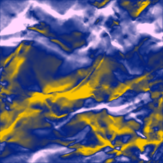
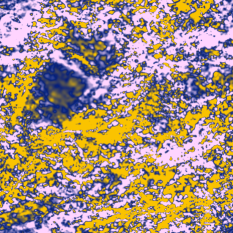
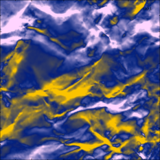
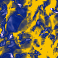
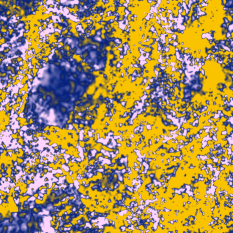
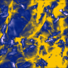
Figure 4.7: The column integrated $x$ & $z$ (top, bottom) magnetic field components using fixed $\alpha_{\text{B}}=1$ (left), the PM05 switch (centre), and the new switch (right) after two turbulent turnover times (i.e., the regime of fully developed turbulence). The magnetic field structure using the previous switch is dominated by unphysical noise due to the shocks failing to be captured (centre), whereas the new switch is able to capture the shocks and the magnetic field retains its physical structure (right).

The column integrated $x$ & $z$ components of the magnetic field are shown in Figure 4.7 at $t=2$ turbulent turnover times. The PM05 switch fails to raise $\alpha_{\text{B}}$ to appreciable levels ($\alpha_{\text{B}}\sim 10^{-5}$), and as demonstrated in Figure 4.7, the shocks in the magnetic field fail to be captured. This leads to break-up of the shocks, causing unphysical magnetic field growth until such a time as the field is strong enough to activate the switch. By contrast, the new switch is invariant to field strength meaning that it turns on resistivity in the shocked regions and the shocks are captured.

We also found for this simulation that using the averaged Alfvén speed as the signal velocity for resistivity produces the same behaviour (shocks breaking apart). In this instance, it is due to the large disparity between the Alfvén and sound speed meaning that the applied resistivity is too weak to capture the strong shocks properly. With the fast MHD wave speed in the signal velocity (Equation 4.5), the shocks are captured correctly.

4.3 Generalisation to other dissipation terms

In this section, we extend the design concept of the new artificial resistivity switch to the artificial viscosity and thermal conductivity dissipation terms, constructing new switches based on the general idea of a normalised shock indicator (see also Tricco and Price, 2013a).

4.3.1 New artificial viscosity switch

For the new artificial viscosity switch, we continue to use $-\nabla\cdot{\bf v}$ as the shock indicator as in the Morris and Monaghan (1997) approach. It would be unwise to use $|{\bf v}|$ for the normalisation as this would break Galilean invariance. Instead, the fast MHD wave speed is used (or sound speed in pure hydrodynamics), relating the quantity to the Mach number.

It is also important that artificial viscosity is applied to the wake of the shock to reduce post-shock oscillations of the particles (as discussed in Section 2.2.10.1). Therefore, $\alpha$ is reduced over time using an integrated decay term like in the Morris and Monaghan (1997), Cullen and Dehnen (2010), and Read and Hayfield (2012) approaches.

The resulting switch is therefore to set

$$\alpha_{a}=-\frac{h_{a}\nabla\cdot{\bf v}_{a}}{v_{\rm mhd}}$$ (4.8)

when greater than the current value of $\alpha_{a}$, otherwise $\alpha_{a}$ is reduced on the next time step according to

$$\frac{{\rm d}\alpha_{a}}{{\rm d}t}=-\frac{\alpha_{a}}{\tau},$$ (4.9)

where $\tau=h/\sigma_{v}v_{\rm mhd}$ has the same meaning as in the Morris and Monaghan (1997) switch (Equation 2.99). By following the considerations outlined above, this viscosity switch is quite similar in principle to the switch of Cullen and Dehnen (2010), albeit with a simpler version for Equation 4.8.

4.3.2 New thermal conductivity switch

A switch for thermal conductivity can be constructed by analogy to Equation 4.1. The gradient of thermal energy is chosen to detect discontinuities, setting

$$\alpha_{u,a}=\frac{h_{a}|\nabla u_{a}|}{|u_{a}|}.$$ (4.10)

As with artificial resistivity, it is expected that thermal conductivity only needs to be applied at the location of the discontinuity since there is no worry of oscillations in particle motion. Therefore, no time-integrated decay term is used.

4.3.3 Tests of artificial viscosity and thermal conductivity switches

The efficacy of the new artificial viscosity and thermal conductivity switches are examined using a standard Sod shocktube test, and a setup producing Kelvin-Helmholtz instabilities.

4.3.3.1 Viscosity: Sod shocktube

The Sod shocktube (Sod, 1978) has become a canonical test for hydrodynamic shocks. It consists of a fluid with a discontinuity in the density and pressure that sends a shock wave into the low density medium and a rarefaction into the high density medium, with a contact discontinuity in the centre. Artificial viscosity is required in this test in order to treat the shock wave.

The simulation has left state ($x<0$) $\rho=1$ and $P=1$ in contact with a fluid of $\rho=0.125$ and $P=0.1$ ($x>0$) with $\gamma=5/3$. Both states have zero initial motion. The shocktube is simulated in 1D using $1000$ and $125$ particles for the two states, respectively. Thermal conductivity is used with fixed $\alpha_{u}=1$, using the Price (2008) switch (see Section 2.2.11.3).

Results at $t=0.2$ are presented in Figure 4.8 along with the solution calculated from a Riemann solver. The SPH solution agrees well with the Riemann solution, though there are small post-shock oscillations in the velocity field, which may also be noticed when using the Morris and Monaghan (1997) switch (see also Cullen and Dehnen 2010). These can be reduced by adjusting the decay timescale for $\alpha_{\rm AV}$. The contact discontinuity is spread over $\sim 12$ particles, but this is not related to the artificial viscosity scheme.

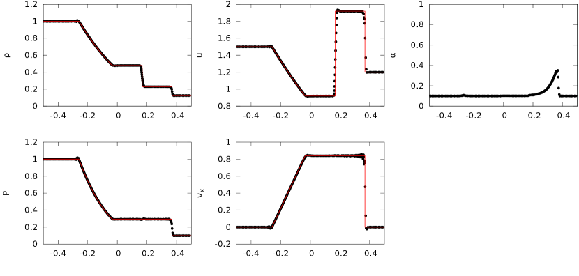
Figure 4.8: Sod shocktube results at $t=0.2$ using the new viscosity switch described in Section 4.3.1. The black circle are values from the particles with the red line the Riemann solution.

4.3.3.2 Thermal conductivity: Kelvin-Helmholtz instability

Kelvin-Helmholtz instabilities have been studied many times with SPH (e.g., Agertz et al., 2007; Price, 2008; Valcke et al., 2010; McNally et al., 2012; Hubber et al., 2013). The instability occurs when there is a velocity shear in a fluid, causing turbulence to form along the interface. An important aspect to simulating this correctly in SPH is application of thermal conductivity to treat thermal energy discontinuities across the interface. If ignored, spurious pressure is generated preventing the fluid from mixing properly. We use this test to investigate the ability of the new thermal conductivity switch to allow mixing of the fluids across the interface, and produce the “curls” which are emblematic of Kelvin-Helmholtz instabilities.

The test performed here follows the initial set up of Price (2008). The fluid contains two regions in a 2:1 density contrast. The domain is $x,y=[-0.5,0.5]$ and periodic boundary conditions are used creating two interfaces along which Kelvin-Helmholtz instabilities form. The initial density profile is

$$\rho=\begin{cases}2&\text{ }|y|<0.25,\\ 1&\text{ }|y|>0.25.\end{cases}$$ (4.11)

The two regions are in pressure equilibrium with uniform $P=2.5$ with $\gamma=5/3$. The $x$-velocity is $-0.5$ for the $\rho=2$ region, and $0.5$ for the $\rho=1$ region. The $y$-velocity is zero, however the $n=4$ instability is seeded with a perturbation across the interfaces by

$$v_{y}=\begin{cases}A\sin[-2\pi(x+0.5)/\lambda]&+0.225<y<+0.275,\\ A\sin[2\pi(x+0.5)/\lambda]&-0.225<y<-0.275,\end{cases}$$ (4.12)

where $A=0.025$ and $\lambda=1/6$.

The characteristic growth timescale of the instability depends on the densities of both fluids and the relative velocity shear. For an incompressible fluid, the timescale is (Chandrasekhar, 1961)

$$\tau_{\rm KH}=\frac{\lambda(\rho_{1}+\rho_{2})}{(\rho_{1}\rho_{2})^{1/2}|v_{1}-v_{2}|},$$ (4.13)

where $\rho_{1}$ and $v_{1}$ are the density and velocity of one fluid, with $\rho_{2}$ and $v_{2}$ the density and velocity of the other. For this calculation, the Kelvin-Helmholtz growth timescale is $\tau_{\rm KH}\approx 0.35$.

The particles are initially arranged on triangular lattices. A total of $454184$ particles are used, with a particle spacing of $\Delta=1/512$ in the low density region and $\Delta=1/724$ in the high density region. The Morris and Monaghan (1997) switch (Equation 2.99) is used for artificial viscosity. The initial thermal energy is calculated using the density of the particles so that the pressure is constant across the interfaces. The quintic spline has been used.

The calculations were run using four different thermal conductivity switches: two based on pressure discontinuities and two on the relative velocity between particles (as motivated by methods such as Wadsley et al. 2008; Shen et al. 2010; Valdarnini 2012; Read and Hayfield 2012). The four thermal conductivity switches tested are: the normalised thermal gradient switch developed in Section 4.3.2; the divergence of the velocity, $v_{\rm sig}^{u}=|{\bf v}_{ab}\cdot\hat{\bf r}_{ab}|$, as used by Valdarnini (2012); the curl of the velocity, $v_{\rm sig}^{u}=|{\bf v}_{ab}\times\hat{\bf r}_{ab}|$, which should perform better at detecting shear motions; and the approach of Price (2008) to set $v_{\rm sig}^{u}=\sqrt{|P_{a}-P_{b}|/\overline{\rho}_{ab}}$. A calculation was performed with no thermal conductivity to act as a reference.

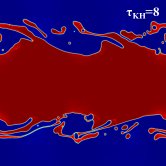
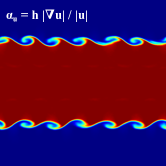
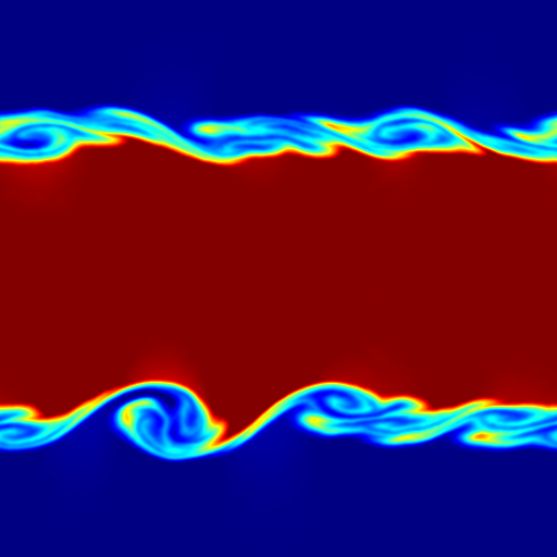
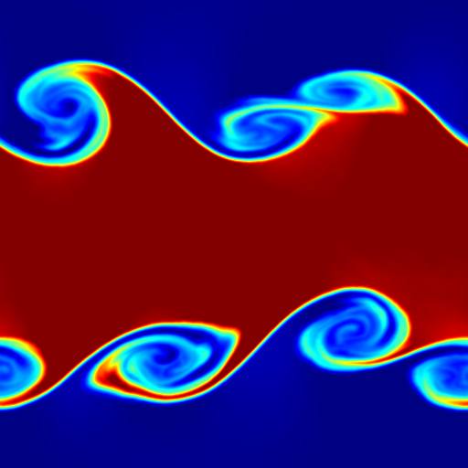
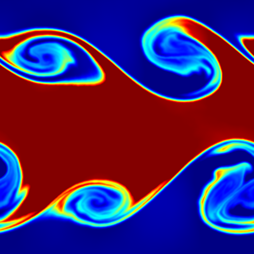
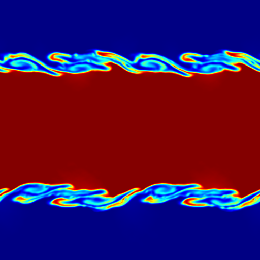
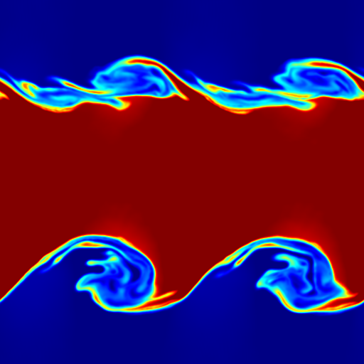
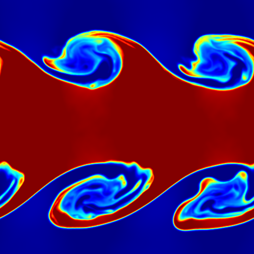
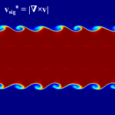
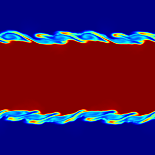
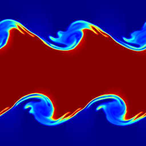
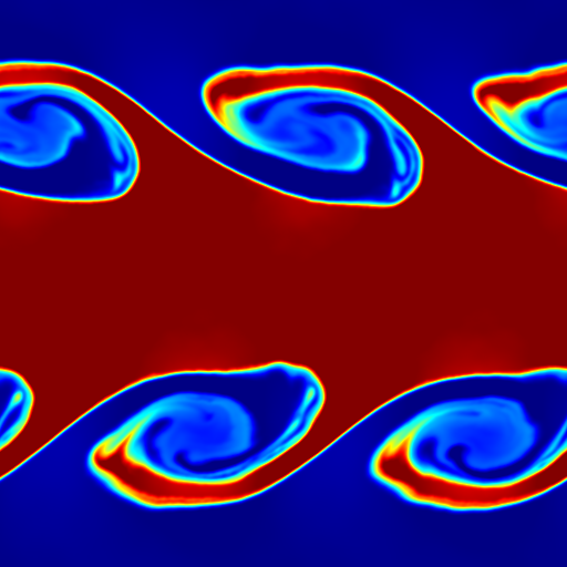
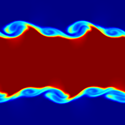
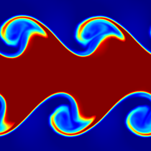
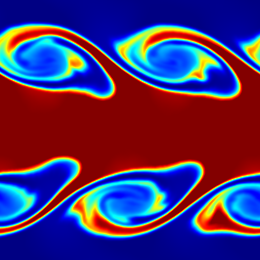
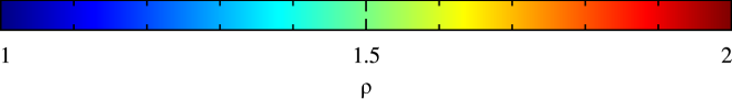
Figure 4.9: Results of the Kelvin-Helmholtz instability test using no thermal conductivity (first row), then thermal conductivity with the following switches: $\alpha_{u}=h|\nabla u|/|u|$ (second row), $v_{\rm sig}^{u}=|{\bf v}_{ab}\cdot\hat{\bf r}_{ab}|$ (third row), $v_{\rm sig}^{u}=|{\bf v}_{ab}\times\hat{\bf r}_{ab}|$ (fourth row), and $v_{\rm sig}^{u}=\sqrt{|P_{a}-P_{b}|/\overline{\rho_{ab}}}$ (fifth row). Times are shown for $\tau_{\text{KH}}=2,4,6,8$ (left to right). Instabilities form along the 2:1 density contrast interfaces due to a velocity shear. Without thermal conductivity, the discontinuity in thermal energy is untreated, leading to a spurious pressure that prevents mixing of the two regions. All conductivity switches allow the instability to form.

Figure 4.9 shows the results of the calculations at $\tau_{\text{KH}}=2,4,6,8$. The results without thermal conductivity demonstrate its necessity. The spurious pressure across the interface cause globs of the high density fluid to stretch and break off without mixing and the instability fails to correctly develop. All results using thermal conductivity are qualitatively similar — six small curls are formed along either interface, which coalesce to form two large curls. The interior structure of the large curls differ between the cases, which is to be expected due to the non-linearity of the problem. This initial configuration is known to be unstable at all wavelengths (Chandrasekhar, 1961), thus while the $\lambda=1/6$ wavelength is seeded and most prominent, secondary instabilities at other wavelengths will occur.

We find that the Price (2008) switch leads to the most symmetrical result. The new thermal gradient switch is effective at promoting mixing along the interface, though the curls at $\tau_{\rm KH}=8$ are all of different sizes. The $|{\bf v}_{ab}\cdot\hat{\bf r}_{ab}|$ is similar in that the curls are dissimilar in shape. In contrast, the $|{\bf v}_{ab}\times\hat{\bf r}_{ab}|$ has curls which are more uniform and like that of the Price (2008) switch case. We conclude that using a switch based on the thermal gradient is effective at promoting mixing, but performing further tests, particularly ones that have quantitative convergence, would be desirable. Our results do suggest, though, that a switch based on the curl of the velocity field performs better than one based on the divergence of the velocity.

4.4 Summary

We have developed a switch to dynamically regulate the amount of artificial resistivity applied to the magnetic field in smoothed particle magnetohydrodynamics simulations (see also Tricco and Price, 2013b). Since the purpose of artificial resistivity is to model magnetic shocks and discontinuities, the key is to minimise spurious dissipation in smooth parts of the field. Our switch accomplishes this by setting the artificial resistivity parameter $\alpha_{\text{B}}$ equal to the dimensionless quantity $h|\nabla{\bf B}|/|{\bf B}|$. This yields a simple, powerful and robust method for reducing magnetic dissipation away from shocks with no loss in shock-capturing ability. Importantly, it responds appropriately at all magnetic field strengths, a particular improvement over the PM05 switch which was found to inadequately capture shocks in weak fields.

Alternative switches using the second derivative of the magnetic field were also investigated, in particular $h|\nabla^{2}{\bf B}|/|\nabla{\bf B}|$ and $h^{2}|\nabla^{2}{\bf B}|/|{\bf B}|$. The key requirement to their success is a high order estimate of the second derivative, otherwise noise from particle disorder overwhelms the derivative estimate and causes excessive dissipation. Obtaining this higher order estimate, however, adds significant computational expense. In general, we recommend our first derivative switch for normal use since it is simple, yet performs robustly and effectively.

Three shocktube tests (Sections 4.2.1, 4.2.2, and 4.2.3) were used to establish that the switch correctly models a range of shock phenomena, including fast and slow shocks, fast and slow rarefactions, rotational discontinuities, and compound shock structures. The L1 error of the magnetic field profiles for all tests was lower when using this new switch compared to using the PM05 switch. These tests also demonstrated that the our new divergence cleaning algorithm is stable and robust in shocktube problems, in contrast to the version proposed by Stasyszyn et al. (2013).

In Section 4.2.4, the propagation of a travelling Alfvén wave was used to gauge the switch’s ability to reduce unwanted dissipation in situations not involving discontinuities, and was found to result in maximum $\alpha_{\text{B}}$ values 10$\times$ smaller than the PM05 switch ($\sim 0.02$ compared to $\sim 0.22$). After 6 periods, the amplitude of the wave using the PM05 switch was four times lower than using the new switch.

The Orszag-Tang vortex was used in Section 4.2.5 to examine the performance of the new switch when there are multiple interacting shocks, producing regions of $\alpha_{\text{B}}\sim 1$ that closely traced the shock lines. The new switch was found to decrease the spurious dissipation in smooth regions compared to the PM05 switch, leading to the subtle magnetic features being more sharply defined, equivalent to running the test at higher resolution.

Finally, in Section 4.2.6, a simulation of Mach 10 MHD turbulence was used to demonstrate the switch’s ability to capture magnetic shocks when a weak magnetic field is combined with strong hydrodynamic shocks. The PM05 switch was found to fail for the low field strengths present in this problem, causing the magnetic field to be dominated by unphysical noise. With the new switch the magnetic shocks remain coherent.

We found that it is very important to use the fast MHD wave speed as the characteristic signal velocity for artificial resistivity. Using the Alfvén speed as the characteristic signal velocity, as proposed by Price (2012), was found to inadequately capture fast MHD shocks in the highly super-Alfvénic regime, leading to unphysical effects (Figure 4.7).

In Section 4.3, the design concept of the switch was generalised for use with artificial viscosity and thermal conductivity (see also Tricco and Price, 2013a). The new artificial viscosity switch needed an integrated decay term to treat post-shock oscillations of particle motion, yielding a switch similar to that of Cullen and Dehnen (2010). Performance on a Sod shocktube was in agreement with the Riemann solution. The thermal conductivity switch was tested with a simulation of the Kelvin-Helmholtz instability. It was able to mitigate the spurious pressure force across the interface, forming the characteristic billowing curls, however had noticeable asymmetries. Results were compared against other thermal conductivity switches: the Price (2008) pressure difference formulation, and the divergence and curl of the velocity field. We found that the Price (2008) and the velocity curl switches performed best for this problem, in that they had the most mixing and retained the symmetry of the problem.

Our new switch is widely applicable to astrophysical SPMHD simulations, in particular for simulations involving weak fields such as in galaxy and cosmological simulations, and also for dynamo processes. In every case we tested, it produced lower magnetic dissipation than the PM05 switch, making it possible to achieve higher magnetic Reynolds numbers in simulations of the interstellar and intergalactic medium. The new switch thus supercedes the PM05 in every respect.

Declaration for Chapter 5

Declaration by Candidate

In the case of Chapter 5, the nature and extent of my contribution to the work was the following:

Nature of Contribution	Extent of Contribution (%)
First author of 2014, “A comparison between grid and particle methods on small-scale dynamo amplification of magnetic fields in supersonic turbulence”, Submitted to ApJ.	90

The following co-authors contributed to the work:

Name	Nature of Contribution	Extent of Contribution (%) for student co-authors
Daniel Price	Second author, PhD supervisor
Christoph Federrath	Third author, performed grid based calculations

The undersigned hereby certify that the above declaration reflects the nature and extent of the candidate’s and co-author’s contributions to this work.

Chapter 5 Turbulent dynamo amplification of magnetic fields

Supersonic turbulence regulates star formation (Mac Low and Klessen, 2004; McKee and Ostriker, 2007), producing the dense filaments that permeate molecular clouds along which dense cores and protostars form (e.g., Larson, 1981; Hartmann, 2002; Elmegreen and Scalo, 2004; Hatchell et al., 2005; André et al., 2010; Peretto et al., 2012). That the turbulence is magnetised cannot be ignored. Magnetic fields are no longer thought to prevent gravitational collapse altogether, but may still determine the rate and efficiency of star formation, even with weak magnetic fields i.e., super-Alfvénic turbulence (Nakamura and Li, 2008; Lunttila et al., 2009; Price and Bate, 2008, 2009; Padoan and Nordlund, 2011; Federrath and Klessen, 2012).

Magnetic fields grow in a turbulent environment by the conversion of kinetic energy into magnetic energy. This type of dynamo is small-scale, operating near the dissipation scale. It is there that the smallest motions can efficiently grow the magnetic field through rapid winding and twisting of the magnetic field lines, with the magnetic field as a whole growing exponentially through a reverse cascade from small to large scales (see review by Brandenburg and Subramanian, 2005). The magnetic field will saturate first on small scales due to the back-reaction of the Lorentz force on the turbulent flow, after which it enters a linear or quadratic growth phase, until the field finally reaches saturation on all scales (Cho et al., 2009; Schleicher et al., 2013). The growth rate is determined by the physical viscosity and magnetic resistivity of the plasma, which can be expressed as dimensionless numbers: the kinematic Reynolds number ($\mathrm{Re}$), the magnetic Reynolds number ($\mathrm{Rm}$), and the ratio of the two, the ‘magnetic Prandtl number’, ${\rm Pm}={\rm Rm}/{\rm Re}$ (Schekochihin et al., 2004a; Brandenburg and Subramanian, 2005; Schober et al., 2012a, b; Bovino et al., 2013). Using a large set of numerical simulations, Federrath et al. (2011) found that the dynamo growth rate also depends sensitively on the compressibility of the plasma, parameterised by the turbulent Mach number, and is more efficient for turbulence driven by solenoidal (rotational) flows rather than compression.

These processes involve highly non-linear dynamics and complex behaviours, making analytic study difficult (with notable exceptions; Sridhar and Goldreich 1994; Goldreich and Sridhar 1995). Furthermore, observations of magnetic fields in molecular clouds are time consuming and only yield field directions in the plane of the sky and magnitudes along the line of sight (e.g., Crutcher, 1999; Bourke et al., 2001; Heiles and Troland, 2005; Troland and Crutcher, 2008). Numerical simulations complement analytics and observations. It is therefore important to compare results from different codes and to establish the conditions under which those results are representative of the physical processes involved.

There have been several major code comparison projects related to supersonic turbulence. Tasker et al. (2008) compared two grid codes (Enzo, Flash) and two particle-based codes (Gadget2, Hydra) on simple test problems involving strong hydrodynamic shocks, finding comparable results when the number of particles were roughly equal to the number of grid cells. Kitsionas et al. (2009) studied decaying, supersonic, hydrodynamic (non-magnetised) turbulence, comparing four grid codes (Enzo, Flash, TVD, Zeus) and three particle codes (Gadget, Phantom, Vine). They found similar velocity power spectra and density probability distribution functions (PDF) when the number of resolution elements was comparable, though the particle codes were found to be more dissipative. Kritsuk et al. (2011) compared decaying, supersonic turbulence with magnetohydrodynamics (MHD) using nine different grid codes: Enzo, Flash, KT-MHD, LL-MHD, Pluto, PPML, Ramses, Stagger, and Zeus. They found that all methods produced physically consistent results, with the quality of results improved with higher-order numerical solvers, and by exactly rather than approximately maintaining the divergence-free constraint on the magnetic field.

A key shortcoming of both the Kitsionas et al. (2009) and Kritsuk et al. (2011) comparisons was that they studied decaying turbulence. Interpolating the initial conditions obtained by driving the turbulence in one code introduced discrepancies between codes before the numerical experiments even started. Those discrepancies in the initial conditions were most severe between grid and particle methods, but also for different grid discretisations (e.g. staggered vs. unstaggered meshes), and is problematic in the MHD case since one must enforce $\nabla\cdot{\bf B}=0$. Furthermore, it is difficult to obtain a statistically significant sample of simulation snapshots in the absence of a statistical steady-state, given that supersonic turbulence decays within a few crossing times. This limitation means that intermittent, intrinsic fluctuations of the turbulence largely exceeded systematic differences in the numerical schemes, which we want to quantify.

Price and Federrath (2010a) (hereafter PF10) addressed these issues in a hydrodynamic comparison by using driven instead of decaying turbulence, enabling the calculations to start from a well-defined initial state and allowing time-averaged statistical comparisons. They compared two codes: the grid code, Flash, and the smoothed particle hydrodynamics (SPH) code, Phantom, taken as broadly representative of the two classes of hydrodynamical methods used in astrophysics: grid-based versus particle-based. Both codes used exactly the same turbulence driving routine and sequence to prevent any bias from different implementation of driving or from different initial conditions: both codes start with a gas of uniform density at rest. They found similar resolution requirements to previous studies, but that grid-based methods were better at resolving volumetric statistics at a given resolution, while SPH better sampled density-weighted quantities. However, this comparison was limited to hydrodynamic turbulence.

Phantom was initially entered for the Kritsuk et al. (2011) comparison, but was withdrawn because, at the time, the best approach to maintaining $\nabla\cdot{\bf B}=0$ in smoothed particle magnetohydrodynamics (SPMHD) used the Euler potentials, ${\bf B}=\nabla\alpha\times\nabla\beta$ (Price and Bate, 2007; Rosswog and Price, 2007). This formulation was incompatible with the initial conditions used in the comparison (see discussion in Rosswog and Price 2007) and excludes dynamo processes by construction because the Euler potentials method cannot represent and follow wound-up magnetic field structures (Price and Bate, 2008; Brandenburg, 2010; Price, 2012). Results evolving the magnetic field directly were poor (no $\nabla\cdot{\bf B}$ control). These difficulties have now been resolved. In Chapter 3, we developed a new constrained hyperbolic divergence cleaning method for SPMHD that maintains $\nabla\cdot{\bf B}=0$ to sufficient accuracy for a wide range of problems, without the topological restrictions associated with the Euler potentials. In particular, this has enabled successful simulations of jets and outflows during protostar formation (Price et al., 2012; Bate et al., 2014b) which involve winding up of magnetic fields. In Chapter 4, we have further improved the magnetic shock-capturing algorithm, particularly when dealing with weak magnetic fields. Hence, it is now possible to simulate magnetic dynamos with SPMHD.

This chapter presents a comparison between Flash and Phantom on the direct numerical simulation of small-scale dynamo amplification of a weak magnetic field from driven, supersonic turbulence. We investigate the dependence of the growth rate on the numerical resolution, a measure of the numerical dissipation properties of each code. We also study the statistical properties of super-Alfvénic turbulence after the magnetic field has saturated. The comparison is otherwise identical to PF10, using the same driving routine and Mach number, so that any differences are from the MHD implementations only. In order to capture the growth of the magnetic field and obtain time-averaged statistics after it has saturated, the calculations are evolved for one hundred crossing times, in contrast to only ten in PF10. This is another motivation for performing driven turbulence calculations, rather than revisit the decaying turbulence simulations of the Kritsuk et al. (2011) comparison. Such simulations can only be evolved for a few turbulent crossing times before the turbulence decays.

In Section 5.1, we describe the equations to be solved, the initial state, and the driving routine. Section 5.2 introduces the numerical details of Flash and Phantom. Results of the simulations are analysed in Section 5.3, focusing on the transient phase during which the turbulence is formed (Section 5.3.1), the growth of magnetic energy from the turbulent dynamo (Section 5.3.2), and after the magnetic energy reaches its saturation value (Section 5.3.3). A summary of our results is presented in Section 5.4.

5.1 Comparison details

The aim is to compare grid and particle methods on the growth and saturation behaviour of a magnetic field that is amplified by a turbulent dynamo. We solve the ideal MHD equations (Section 2.1.3). The continuum equations have zero viscous and resistive dissipation (hence ideal). Since the growth rate of the small-scale dynamo is set by the dissipation of the system, it may seem strange to perform a comparison using the ideal MHD equations. However, it is common to use the ideal MHD equations for astrophysical simulations, and some amount of dissipation is inevitably introduced when solving these equations numerically. In grid-based methods, numerical dissipation is introduced by the discretisation of the advection term in the material derivative. By contrast, in Lagrangian particle-based methods the material derivative is computed exactly. The shock-capturing scheme is the other source of numerical dissipation. Modern grid-based methods use Riemann solvers which introduce a numerical dissipation related to the accuracy of the shock reconstruction. The approach in particle methods is to explicitly add viscous and resistive terms in order to capture shocks, using switches to tune the dissipation to the relevant discontinuity. Since the small-scale turbulent dynamo is sensitive to both viscous and resistive dissipation, and the ratio of these two (${\rm Pm}=\nu/\eta$), it can be used to quantify and compare the numerical dissipation between codes.

The initial state is simple so that both codes start from the same initial conditions. The system is initialised with a uniform density field, $\rho_{0}=1$, and zero velocity field. The system is contained in a periodic box of length $L=1$. An isothermal equation of state, $P~{}=~{}c_{\rm s}^{2}\rho$, is used to calculate the pressure with sound speed $c_{\rm s}=1$. The magnetic field is set to $\sqrt{2}\times 10^{-5}$ in the $z$ - direction. With $\mu_{0}=1$, this yields an initial plasma beta, the ratio of thermal to magnetic pressure, of $\beta=P/P_{\rm mag}=10^{10}$.

As in PF10, supersonic turbulence is initiated and sustained at a root mean square (rms) Mach number of $\mathcal{M}=10$ by an imposed driving force generated from an Ornstein-Uhlenbeck process (Eswaran and Pope, 1988; Schmidt et al., 2009; Federrath et al., 2010). This is a stochastic process with a finite autocorrelation timescale. By using this approach, the driving force can be decomposed in Fourier space into longitudinal and solenoidal modes. For this comparison, only the solenoidal component of the force is used, and therefore the turbulence is driven primarily by vorticity rather than compression (see Federrath et al. 2011; Federrath 2013 for a study on the effect of different driving). However, 1/3 of the kinetic energy will still be contained in compressive modes due to the high Mach number of the turbulence (Pan and Scannapieco, 2010; Federrath et al., 2010).

Consistency of the driving pattern between codes is achieved by pre-generating the time-sequence of the Ornstein-Uhlenbeck modes, with both codes reading the pattern from file. The driving is at large scales, with a parabolic weighting of modes between $k_{\rm min}=1$ and $k_{\rm max}=3$, with smaller structures forming through turbulent cascade. The autocorrelation timescale is $1t_{\rm c}$, with $t_{\rm c}$ as defined in Equation 5.1. The input parameters used to generate the pattern file are specified in Table 5.1. The stirring energy is used to obtain the variance of the Ornstein-Uhlenbeck process, corresponding to the autocorrelation time and energy input rate.

Table 5.1: Stirring Routine Input Parameters.

Parameter	Value
spectral form	1 (Parabola)
solenoidal weight	1
stirring energy	8.0
autocorrelation time	0.05
minimum wavenumber	6.28
maximum wavenumber	18.90
original random seed	1

The relevant physical timescale is the turbulent crossing time, which we define according to

$$t_{\rm c}\equiv\frac{L}{2\mathcal{M}c_{\rm s}},$$ (5.1)

corresponding to $t_{\rm c}=0.05$ in code units. The turbulence is simulated for 100 crossing times, covering the full growth phase of the dynamo up until the magnetic energy reaches its saturation level, with at least half of the total time spent in the saturation phase. The set of simulations use $128^{3}$, $256^{3}$, and $512^{3}$ resolution elements (grid points and particles, respectively).

5.2 Numerical codes and methods

We compare the codes Flash and Phantom. Both solve the ideal MHD equations but with fundamentally different numerical approaches: Flash discretises all fluid variables into fixed grid points, whereas Phantom discretises the mass of the fluid into a set of Lagrangian particles that move with the fluid velocity. We take these two codes to be representative of the general class of Eulerian, grid-based methods (Flash) and Lagrangian, particle-based methods (Phantom).

5.2.1 Flash

Flash is a grid-based code using a finite volume scheme for solving the MHD equations (Fryxell et al., 2000; Dubey et al., 2008). Although Flash can be used with adaptive mesh refinement (AMR, Berger and Colella, 1989), our simulations employ a fixed and uniform cartesian grid for simplicity. We here use Flash with the HLL3R approximate Riemann solver for ideal MHD, based on a MUSCL-Hancock scheme (Waagan et al., 2011). This is a predictor-corrector scheme and is second-order accurate in both space and time. Waagan et al. (2011) further show that this MHD scheme maintains $\nabla\cdot{\bf B}\sim 0$ to within negligible errors, by using divergence cleaning in the form of the parabolic cleaning method of Marder (1987) (see also Dedner et al., 2002). The MHD solver is particularly efficient and robust, because it uses a relaxation technique that guarantees positive density and gas pressure and thus avoids unphysical states, by construction.

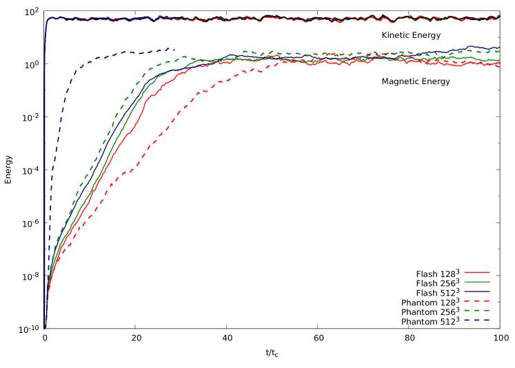
Figure 5.1: Growth and saturation of the magnetic energy for Flash and Phantom at resolutions of $128^{3}$, $256^{3}$, and $512^{3}$. The top lines are the kinetic energy for the six calculations. Flash has similar growth rates across the resolutions simulated, while Phantom exhibits faster growth rates with increasing resolution. This resolution dependence is a consequence of the artificial dissipation terms. Both codes saturate the magnetic energy at similar levels.

5.2.2 Phantom

Phantom is a smoothed particle magnetohydrodynamics (SPMHD) code. The MHD equations (Equations 2.22–2.24) are implemented as described in Price and Monaghan (2004a, b, 2005) and Price (2012), using Børve et al. (2001)’s method of subtracting ${\bf B}(\nabla\cdot{\bf B})$ from the momentum equation to keep the magnetic tensional force stable. This implementation of momentum and induction equations resolves issues related to non-zero $\nabla\cdot{\bf B}$ in a manner that is equivalent to the Powell 8-wave approach (Powell, 1994; Powell et al., 1999).

The divergence of the magnetic field is kept close to zero by using the constrained hyperbolic divergence cleaning method developed in Chapter 3, which is an SPMHD adaptation and improvement of the cleaning algorithm by Dedner et al. (2002). The cleaning wave speed is set to the local fast MHD wave speed. During the course of this work, it was found that if the wave speed included the term involving the relative velocity of particles (as in the artificial viscosity), then the individual timestepping scheme could introduce significant errors to the magnetic field. This occurred when particles were interacting on timestep bins that were spaced too far apart. Using a timestep limiter (i.e., Saitoh and Makino, 2009) can prevent these errors, but for these calculations we instead chose the simpler solution of just reducing the cleaning speed by excluding the relative velocity.

Shocks are captured by adding an artificial viscosity, as described by Price and Monaghan (2004a, 2005) and based on the Monaghan (1997) formulation. It is important that the signal velocity, defining the characteristic speed of information propagation, include a term involving the relative motion of particles to prevent particle interpenetration, and it was found by Price and Federrath (2010a) that for Mach 10 shocks, it was necessary to increase this by setting the dimensionless constant $\beta_{\rm AV}=4$ (as opposed to the common $\beta_{\rm AV}=2$). We use the Morris and Monaghan (1997) switch to reduce dissipation away from shocks.

Discontinuities in the magnetic field are treated with an artificial resistivity. Phantom uses the new switch developed in Chapter 4 to reduce dissipation of the magnetic field away from discontinuities. This switch solves problems with the switch proposed by Price and Monaghan (2005), namely that it is able to capture shocks when the sound speed is significantly higher than the Alfvén speed (i.e., in the super-Alfvénic regime when the magnetic field is very weak). This is done by using the dimensionless quantity $h|\nabla{\bf B}|/|{\bf B}|$, which measures the relative strength of the discontinuity in the magnetic field.

The smoothing length (resolution length), $h$, of each particle is calculated in the usual manner by iteration of the density summation with $h=1.2(m/\rho)^{1/3}$ using a Newton-Raphson solver (Section 2.2.2). This means that the numerical resolution scales with the density. For these set of simulations, the resolution increases by $4$–$8\times$ in the highest density regions, with a decrease in resolution of about $2\times$ in the lowest density regions. Timesteps are set individual to each particle in a scheme that is block hierarchical in powers of two, with each particle setting its timestep based on its local Courant condition. Second order leapfrog time integration is used (Section 2.2.12).

5.2.3 Computational cost

The Flash calculations used $90$, $1600$, and $40~{}000$ cpu-hours for the $128^{3}$, $256^{3}$, and $512^{3}$ simulations. The Phantom calculations used $2700$ and $44~{}000$ cpu-hours for the $128^{3}$ and $256^{3}$ simulations, with the $512^{3}$ calculation using $125~{}000$ cpu-hours for $t=0\to 20$. It is expected that each factor of 2 increase in resolution should increase the computational expense by $16\times$, since there are $8\times$ more resolution elements and the Courant condition should reduce the timestep by half, and both codes exhibit a scaling behaviour that is close to this. For Phantom, the particles are spread over $\sim 6$, $7$, and $8$ individual timestep bins for the $128^{3}$, $256^{3}$, and $512^{3}$ resolution calculations, respectively. Approximately $35\%$ of the computational expense in the Phantom calculations is spent on neighbour finding. The driving routine adds negligible computational expense ($\sim 2\%$ of overall cpu-hours). As in PF10, we find that the $256^{3}$ Phantom calculation takes approximately an equivalent amount of computational time as the $512^{3}$ Flash calculation.

5.2.4 Analysis methods

5.2.4.1 Power spectra

Power spectra are calculated using the same analysis tool for both codes to ensure that results are comparable. The Flash data is directly analysed with this tool, while the power spectrum of Phantom data is obtained by interpolating the particles to a grid of double the particle resolution (i.e., $256^{3}$ particles are interpolated to $512^{3}$ grid points). A higher resolution grid is chosen in order to represent the energy contained in the highest density structures, which are up to $4$–$8\times$ higher than the initial resolution. Appendix B investigates the effect of the resolution of the interpolated grid, in addition to the difference between mass and volume weighted interpolation. We found that the magnetic field was satisfactorily represented by a grid which has twice the resolution of the particle calculation.

5.2.4.2 Probability distribution functions

Computing a volume-weighted PDF from grid methods simply involves binning the cells according to the value of the quantity and normalising such that the integral under the PDF is unity. For SPH this is more complicated since the resolution is tied to the mass rather than the volume. PF10 computed the PDF directly from the SPH particles by weighting the contribution of each particle, $i$, by the volume element $m_{i}/\rho_{i}$. Price et al. (2011) later found that this was inaccurate at high Mach number because $\sum_{i}m_{i}/\rho_{i}$ has no requirement that it equals the total volume. Instead, one should interpolate to a fixed volume using the SPH kernel $W$, since $m_{i}/\rho_{i}$ is only meaningful when multiplied by the kernel (since SPH is derived assuming $\sum_{i}m_{i}/\rho_{i}W({\bf r}-{\bf r}_{i},h)=1$). However, interpolation to a fixed grid (e.g. Kitsionas et al., 2009) is also problematic since the resolution in our simulations is 4–8$\times$ higher in the densest regions compared to a fixed grid with the same number of resolution elements. Hence, sampling the high density tail of the SPH calculation would require a commensurably high resolution grid. We follow Price et al. (2011) in using an adaptive mesh to compute the PDF from the SPH particles, where the mesh is refined until the cell size is smaller than the smoothing length. The SPH PDF is then computed and normalised directly from this adaptive mesh.

$128^{3}$	$256^{3}$	$512^{3}$

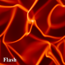
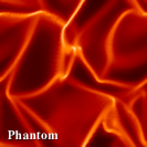
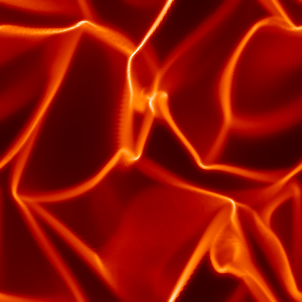
$128^{3}$	$256^{3}$	$512^{3}$

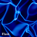
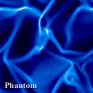
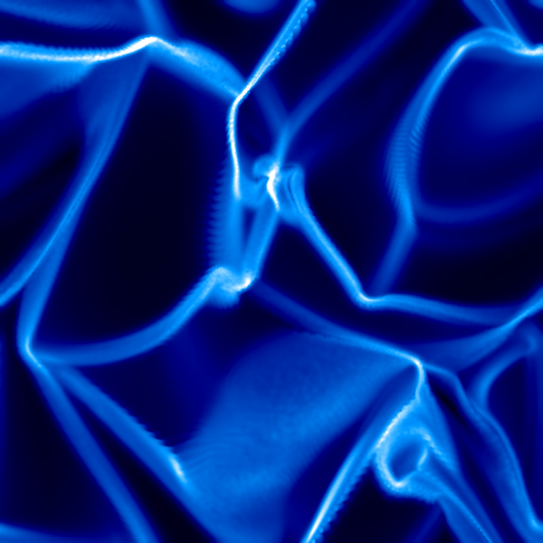
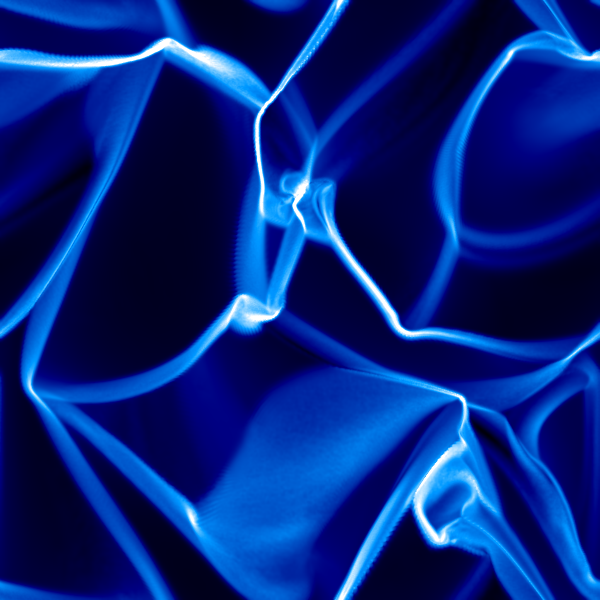
Figure 5.2: Slices of $\rho$ and $|B|$ in the $z=0.5$ mid-plane at $t/t_{\rm c}=1$ during the transient phase. The results from Flash (top row) and Phantom (bottom row) are shown for resolutions of $128^{3}$, $256^{3}$, and $512^{3}$ (left to right). As the resolution is increased, the shock lines become more well defined. The regions with highest magnetic field strength are in the dense shocks.

5.3 Results

Since this comparison uses the same codes, initial conditions, and turbulent driving routine as the hydrodynamic turbulence comparison of PF10, our analysis focuses on the magnetic properties of the turbulence. Hence, analyses performed by PF10 have only been repeated where the addition of magnetic fields would be expected to alter the result (i.e., for the density PDF).

A focus of our analysis is the effect of numerical resolution on the dynamo. Since we assume ideal MHD, the kinetic and magnetic Reynolds numbers vary with resolution. This affects the growth rate and saturation level of magnetic energy, enabling us to contrast the scaling behaviour of the two methods.

The evolution of the magnetic field in the simulations may be divided into three different phases — transient growth, exponential growth, and saturation. These phases can be seen in Figure 5.1 which shows the magnetic and kinetic energy as a function of time for the calculations from both Phantom and Flash using $128^{3}$, $256^{3}$ and $512^{3}$ resolution elements (see legend). We analyse each of these phases in detail below.

5.3.1 Initial transient growth; $t/t_{\rm c}\lesssim 2$

The simulations begin with a brief transient phase while turbulence is generated by the driving routine. Slices of $\rho$ and $|B|$ at $z=0.5$ for $t/t_{\rm c}=1$ are shown in Figure 5.2, shortly after the large shocks created by the driving routine have begun to interact. Magnetic fields are strongest where the density is highest, due to compression of the magnetic field in the shocks. Conversely, the low density regions exhibit relatively weaker magnetic fields.

Approximately half a crossing time is required for the kinetic energy to saturate (see Figure 5.1), though it takes another turbulent crossing time before the turbulence is fully developed. The magnetic energy is amplified by two orders of magnitude during this phase (Figure 5.1). This occurs in two steps: The first ($t/t_{\rm c}\lesssim 1$) is a sharp rise in magnetic energy caused by the formation of large-scale shocks (Figure 5.2). The second occurs during the generation of small-scale structure in the density and magnetic fields caused by the interaction of the shocks. During the second step, from $t/t_{\rm c}\approx 1$–2, the magnetic energy increases exponentially similar to the growth phase (Section 5.3.2), but at a rate higher by a factor of 2–3.

The initial transient growth of the magnetic field is resolution dependent, with higher resolutions yielding higher magnetic energy. For example, the magnetic energy in the $512^{3}$ Phantom calculation increases by an additional $3$–$4$ orders of magnitude compared to the other calculations. We have investigated whether this is a numerical artefact of the timestepping by re-doing the initial phase with a reduction in the Courant factor, and also by using global timesteps instead of individual timesteps. These did not alter our results. Additionally, we have checked if this growth is driven by spurious generation of divergence of the magnetic field by both turning off the hyperbolic divergence cleaning, and conversely by increasing the hyperbolic cleaning wave speed by a factor of $10$ ($10\times$ over-cleaning, see Section 3.5). These showed the same fast transient magnetic field growth, so this is not caused by a high $\nabla\cdot{\bf B}$. Hence, the growth of magnetic energy in the Phantom simulations appears to be physical, originating from the explicitly added dissipation terms rather than occurring due to numerical error or instability.

Table 5.2: Slope of Magnetic Energy Growth and Saturated Energy Values

Calculation	$E_{m}$ growth rate	$\langle E_{\rm k}\rangle_{\text{sat}}$	$\langle E_{\rm m}\rangle_{\text{sat}}$
Flash $128^{3}$	0.30	51.11 $\pm$ 5.51	1.20 $\pm$ 0.31
Flash $256^{3}$	0.32	51.19 $\pm$ 4.81	1.46 $\pm$ 0.20
Flash $512^{3}$	0.32	52.17 $\pm$ 5.15	2.36 $\pm$ 1.02
Phantom $128^{3}$	0.20	50.30 $\pm$ 4.80	1.52 $\pm$ 0.48
Phantom $256^{3}$	0.34	51.17 $\pm$ 5.34	2.31 $\pm$ 0.47
Phantom $512^{3}$	0.71	50.65 $\pm$ 4.20	2.62 $\pm$ 0.19

Flash

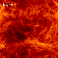
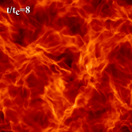
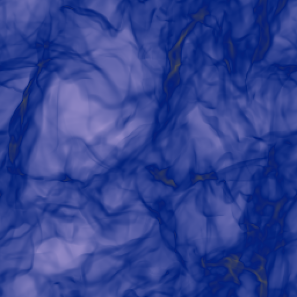
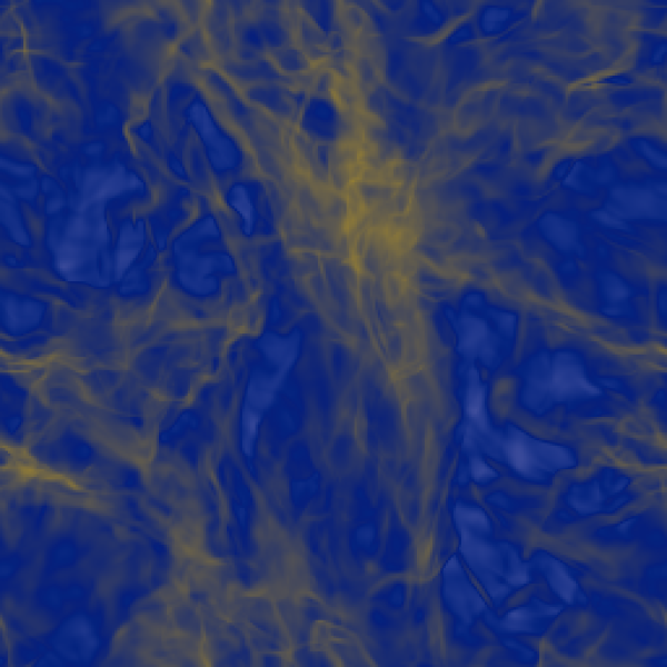
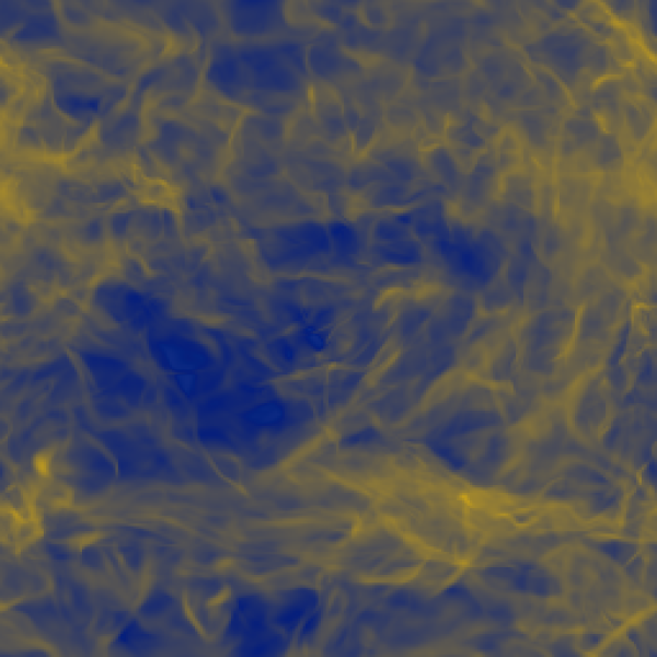
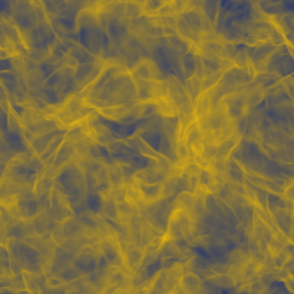
Phantom

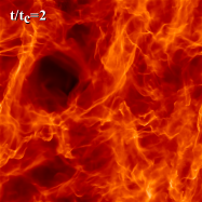
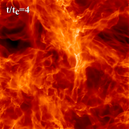
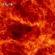
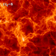
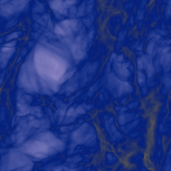
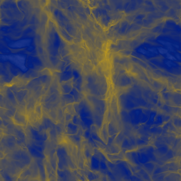
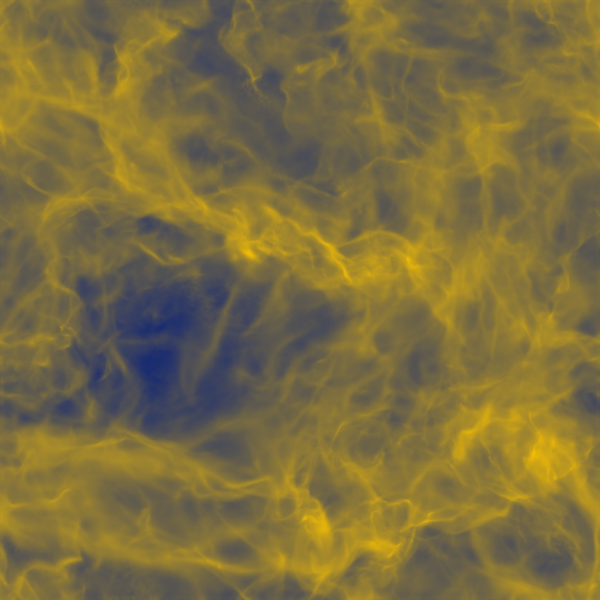
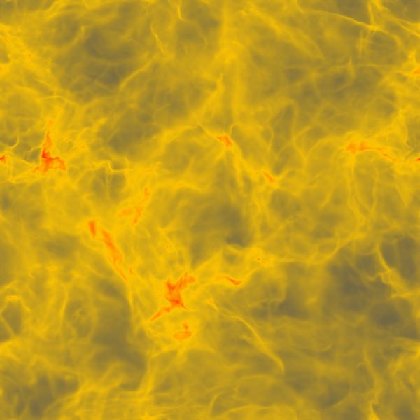
Figure 5.3: $z$-column integrated $\rho$ and $|B|$, defined $<B>=\int|B|{\rm d}z/\int{\rm d}z$, for Flash (top) and Phantom (bottom) at resolutions of $256^{3}$ for $t/t_{\rm c}=2,4,6,8$. The density field has similar structure in both codes at early times, but diverge at late times due to the non-linear behaviour of the turbulence. The magnetic field is strongest in the densest regions, while the mean magnetic field strength also increases with time.

5.3.2 Growth phase; $2\lesssim t/t_{\rm c}\lesssim 10$–$40$

Once the hydrodynamic turbulence is fully developed, the magnetic field is exponentially amplified at a steady rate via the small-scale dynamo. During this phase the magnetic energy is amplified by approximately $8$ orders of magnitude until it reaches its saturation level, occurring when the conversion of kinetic to magnetic energy is balanced by the dissipation of magnetic energy and the back-reaction by the Lorentz force resists further winding of the field. The reservoir of kinetic energy is maintained by continual driving of large-scale motions via the driving routine. The magnetic energy saturates at $t/t_{\rm c}\sim 30$ for all three Flash calculations, but the time of saturation in the Phantom calculations varies from $t/t_{\rm c}=12$ to $t/t_{\rm c}=45$ depending on the resolution. In all cases, the saturation occurs when $v_{\rm A}\sim c_{\rm s}$.

5.3.2.1 Correlation with the density field

Figure 5.3 shows a time sequence of column density and column integrated $|B|$ from $t/t_{\rm c}=2$–$8$, comparing Flash (top figure) and Phantom (bottom figure) calculations at $256^{3}$ since the growth rates are similar at this resolution (c.f. Figure 5.1 and Table 5.2). Both codes show similar patterns in column density and magnetic field for the first few crossing times (left two columns), but eventually the patterns diverge due to the chaotic nature of turbulence (right two columns; this was also found in PF10). Nevertheless, there exists a definite correlation between the density and the magnetic field when compared at a fixed time for each code individually. The mean magnetic field strength can be seen to increase with time in both the low and high density regions.

5.3.2.2 Magnetic energy growth rates

Table 5.2 compares the slope of a line fitted to the magnetic energy for each of the six calculations during the growth phase (defined between $t/t_{\rm c}=3$ and the onset of the slow growth phase).

Analytic studies of the small-scale dynamo have shown that for $\text{Pm}\ll 1$, the growth rate scales with $\text{Rm}^{1/2}$, while for $\text{Pm}\gg 1$, it scales with $\text{Re}^{1/2}$ (Bovino et al., 2013). Theoretical predictions of the growth rate for $\text{Pm}\sim 1$, which is the Prandtl number regime for numerical codes in the absence of explicit dissipation terms, are more uncertain. Federrath et al. (2011) measured the effective Prandtl number in Flash through comparison with calculations with physical dissipation terms, finding that $\text{Pm}\sim 2$. This is in agreement with similar experiments by Lesaffre and Balbus (2007). For Phantom, the effective Prandtl number can be estimated analytically from the artificial dissipation terms, for which we find that $\text{Pm}\sim 1$ for these calculations (see Appendix C for further discussion).

Figure 5.4: Left panel: A $128^{3}$ Phantom calculation where the artificial viscosity and resistivity parameters are systematically increased (no switches are used). With increasing dissipation, the growth rate decreases, producing the same behaviour as changing the resolution. Right panel: Comparing $128^{3}$ Phantom calculations where the viscous and resistive dissipation parameters scale equally ($\alpha=\alpha_{\rm B}$ set to $1$ and $10$) to calculations where one is scaled independent of the other ($\alpha=1$, $\alpha_{\rm B}=10$ and $\alpha=10$, $\alpha_{\rm B}=1$). The growth rate appears to depend upon both Reynolds numbers — specifically, being set by whichever is higher.

To investigate the growth rate dependence on resolution for Phantom, we performed a series of calculations where the dimensionless parameters $\alpha$ and $\alpha_{\rm B}$ in the artificial viscosity and resistivity terms were fixed to different values. We found that the growth rate depended sensitively on the amount of artificial dissipation applied, producing an effect equivalent to changing the resolution (left panel of Figure 5.4). Since the dissipation in Phantom is proportional to resolution, we conclude that the growth rates obtained in our comparison are consistent with the expected resolution scaling of the artificial dissipation terms. Interestingly, the growth rate only changed when both dissipation parameters were varied. Changing only one left the growth rate largely unchanged (right panel of Figure 5.4), suggesting that the growth depends upon the higher of ${\rm Re}$ and ${\rm Rm}$. A worthwhile follow-up would be to compare growth rates with physical dissipation terms that are resolution independent.

Given that the growth rates in the $256^{3}$ calculations are comparable (see Table 5.2 and Figure 5.1), we perform quantitative analysis of our results during the growth phase using the $256^{3}$ resolution calculations. This allows for direct comparison of results.

5.3.2.3 Magnetic energy power spectra

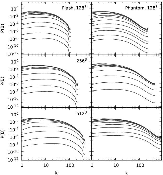
Figure 5.5: Spectra of the magnetic energy during the growth phase for Flash (left) and Phantom (right) for resolutions of $128^{3}$, $256^{3}$, and $512^{3}$ (top to bottom). Each spectral line is sampled at intervals of $5t/t_{\rm c}$ up to $t/t_{\rm c}=50$, except for the $512^{3}$ Phantom run which is sampled every $t/t_{\rm c}$ (from $t/t_{\rm c}=2$–$12$). The magnetic field grows equally at all spatial scales for all calculations.

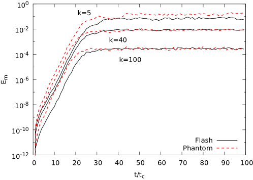
Figure 5.6: Spectra of the magnetic energy at the $k=5$, $40$, and $100$ bands as a function of time for the $256^{3}$ resolution calculations of Flash (black lines) and Phantom (red dashed lines). The growth rate at these different wavenumbers is nearly identical. The saturation level is the same between the two codes for $k=40$ and $100$, with Phantom containing ${\sim}2$ times as much energy in the large-scale $k=5$ band.

That the total magnetic field is growing in strength — and not just in isolated regions — may be quantified by examining the power spectra of the magnetic energy, ${\rm P}(B)$. The magnetic energy spectra during the growth phase for the six calculations is shown in Figure 5.5. The magnetic energy can be seen to grow uniformly at all spatial scales in all six calculations (indicated by the translation of the power spectrum along the y-axis in the plots with minimal change in the shape), behaviour consistent with the small-scale dynamo (Brandenburg and Subramanian, 2005). All of the spectra have the same general shape, with a decrease in spectral energy at and above the driving scale ($k\leq 3$) and a more-or-less flat spectrum (${\rm P}(B)\approx$ constant) between $3<k<10$ for the $128^{3}$ calculations, extending to $k\sim 20$ and $k\sim 40$ for the $256^{3}$ and $512^{3}$ calculations. The dissipation range in the Phantom results extends further to smaller scales than the Flash results for a particular resolution. The maximum in the magnetic energy spectrum in both codes occurs at high wavenumbers, as expected for small-scale dynamos (Cho and Vishniac, 2000; Brandenburg et al., 2012), occurring around the high $k$ end of the ‘relatively’ flat region of the spectra.

Figure 5.6 shows a cross section of the power spectrum evolution at $k=5$, $40$, and $100$ for the $256^{3}$ calculations. These scales were chosen to represent the large, medium, and small-scale structure. This shows that the magnetic field grows in the same manner at all scales in both codes.

5.3.2.4 Approach to saturation

Figure 5.5 shows that the magnetic energy saturates first at small scales. This is characteristic of the small-scale dynamo since this is where magnetic energy is being generated (Cho et al., 2009). It is expected that the magnetic energy will grow linearly at this stage, though for Burgers turbulence, which is closer to the regime our simulations are in, it is expected that the magnetic energy growth will be closer to quadratic (Schleicher et al., 2013). This slow growth phase lasts until the reverse cascade of magnetic energy saturates all spatial scales. This turnover in magnetic energy growth may be clearly seen in the $128^{3}$ and $512^{3}$ Phantom growth curves in Figure 5.1. It is also evident from Figure 5.6 that the magnetic field enters the slow growth phase first at high wavenumbers.

5.3.2.5 PDFs of $B^{2}$

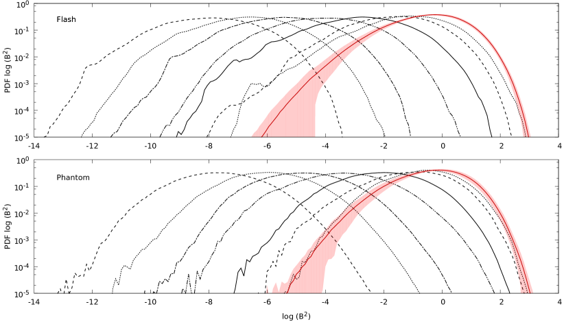
Figure 5.7: PDF of $\log(B^{2})$ during the growth phase, with the red line time averaged during the saturation phase. The top panel shows the Flash calculation, with the bottom panel the Phantom calculation. The PDF has a log-normal distribution during the growth phase, maintaining its width while the peak smoothly translates to higher magnetic field strengths. During the saturation phase, the PDFs of both codes have the similar peaks and high-end tails, with Flash exhibiting a slightly extended low-end tail.

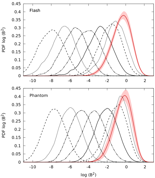
Figure 5.8: PDF of $\log(B^{2})$ during the growth phase, with the red line time averaged during the saturation phase. This is equivalent to Figure 5.7 but on a linearly scaled plot. In the saturation phase, the distribution is skewed with smaller deviation of magnetic field strengths.

Figure 5.7 shows the time evolution of the PDF of $B^{2}$ for the $256^{3}$ calculations. The instantaneous PDFs are shown from $t/t_{\rm c}=4$–$28$ at intervals of $\Delta t=4$, with the time-averaged PDF during the saturation phase given by the red line. The shape of the PDF remains mostly log-normal during the growth phase. As the dynamo amplifies the magnetic field, the PDF maintains its width and shape, with the peak simply translating to higher magnetic field strengths (see also Schekochihin et al., 2004b). In other words, the PDF does not become distorted during the exponential growth phase but only during the slow growth phase as it approaches saturation (see below). This may also be seen in Figure 5.8 which shows the PDF of $B^{2}$ on a linear scale. Figure 5.7 additionally shows that Flash is able to sample lower magnetic field strengths compared to Phantom, which was noted by PF10 in the density PDFs and was attributed to the better weighting of resolution elements towards low density regions in the grid code.

The approach to saturation changes the shape of the PDF of $B^{2}$. It follows a log-normal distribution during the exponential growth phase, but once the dynamo enters the slow growth regime, it is no longer able to amplify the magnetic field on small-scales. Thus, the high-end tail of the distribution remains anchored, and is “squeezed” as the peak and low-end tail continue increasing. This produces a lop-sided distribution (Schekochihin et al., 2004b). Both codes show this behaviour as the magnetic field saturates.

5.3.3 Saturation phase; $15\lesssim t/t_{\rm c}\lesssim 100$

The magnetic energy plateaus once the injection of energy balances its dissipation. While the magnetic field topology changes due to the turbulence during this phase, the magnetic energy remains in a statistical steady state.

5.3.3.1 Magnetic energy saturation level

The mean magnetic energy in the saturation phase is approximately $2$–$4\%$ of the mean kinetic energy (Table 5.2). The mean magnetic energy shows a trend of increasing with resolution, with the $512^{3}$ calculations twice as high as the corresponding calculations at $128^{3}$ (for both Flash and Phantom), though remains within the standard deviation. We note that the $512^{3}$ Phantom calculation is averaged over a shorter time (${\sim}7t_{\rm c}$ compared to $50$–$70t_{\rm c}$), which is reflected by its smaller standard deviation. The $512^{3}$ Flash calculation shows a long-term variation, with a $50\%$ increase in mean energy above $80t_{\rm c}$. This is reflected in the wider standard deviation in this calculation (${\sim}1.0$ compared to $0.2$–$0.3$ in the $128^{3}$ and $256^{3}$ calculations). Overall, while the statistical ranges of mean energy overlap between resolutions, it does appear that Phantom yields higher mean magnetic energy during the saturation phase than Flash at comparable resolution.

The mean magnetic energy in both codes increases with resolution. Given that the Prandtl number in Flash does not scale with resolution (Section 5.3.2), this suggests that the saturation level of the magnetic energy does not depend exclusively on the Prandtl number (Federrath et al., 2014). Instead, our results suggest that it depends on either the kinetic or magnetic Reynolds numbers.

To investigate this further, we performed a set of Phantom simulations, keeping the same artificial viscosity parameters but turning off the artificial resistivity switch developed in Chapter 4 (i.e., using a constant artificial resistivity parameter, $\alpha_{\rm B}=1$), thereby increasing the amount of resistive dissipation. This reduced the mean magnetic energy in the saturation phase at all three resolutions ($128^{3}$: 1.52 to 1.01, $256^{3}$: 2.31 to 1.32, $512^{3}$: 2.62 to 1.40). This, along with the Flash results, suggests that the magnetic Reynolds number is primarily responsible for determining the saturation level of the magnetic field.

5.3.3.2 Alfvénic Mach number

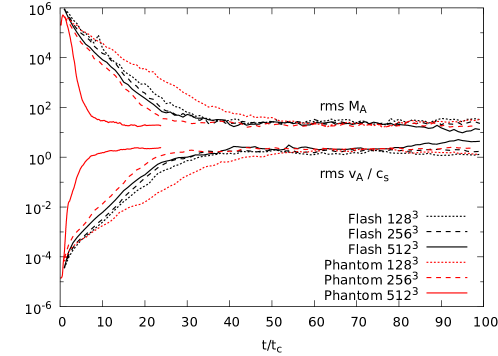
Figure 5.9: Time evolution of the rms Alfvén speed and Alfvénic Mach number. For all calculations, the time averaged rms Alfvén speed in the saturation phase is $v_{\text{A}}\sim 2c_{\rm s}$. The rms Alfvénic Mach numbers is $M_{\text{A}}\sim 20$. This differs noticeably from the rms Alfvén speed divided by the rms velocity (${\sim}5$).

Figure 5.9 shows the time evolution of the rms Alfvén speed, $v_{\rm A}$, and rms Alfvénic Mach number. The rms Alfvén speed in the saturation phase is approximately twice the sound speed. In other words, the turbulence remains super-Alfvénic even once the magnetic field has reached saturation. It is worth noting that the rms $\mathcal{M}_{\rm A}$ in Figure 5.9 is calculated by taking the rms of the local $\mathcal{M}_{\rm A}$ as calculated per grid cell or particle. In the saturation phase, calculating the rms in this manner yields $\mathcal{M}_{\rm A}\sim 20$, which is different (by a factor of 4) to that calculated by dividing the rms velocity ($10$) by the rms $v_{\rm A}$ (yielding ${\sim}5$).

5.3.3.3 Power spectra

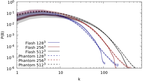
Figure 5.10: Time averaged spectra of the magnetic energy in the saturation phase for Flash (solid lines) and Phantom (dashed lines) at resolutions of $128^{3}$ (blue), $256^{3}$ (red), and $512^{3}$ (black). Shaded regions represent the standard deviation. The Phantom calculations systematically contain more magnetic energy (approximately $2\times$) in large-scale structure ($k<10$) compared to Flash, and have an extended tail at high $k$ due to the adaptive resolution.

Figure 5.10 shows the time-averaged spectra of the magnetic energy from all six calculations in the saturation phase, with the shaded regions showing one standard deviation of the time-average. In each case 50 spectra have been averaged over a minimum of $50t_{\rm c}$. The spectra of Flash and Phantom can be seen to be similar in shape, except that the Phantom calculations contain approximately twice as much magnetic energy in large-scale structure ($k<10$). This is consistent with the higher mean magnetic energy in the Phantom calculations in Table 5.2, indicating that this energy is stored in the largest scales of the field.

The peak of the magnetic energy spectra for both codes is at $k\sim 3$–$4$, occurring just above the driving scale. As the resolution is increased, both codes extend the spectra further towards small scales. The Flash power spectra drop sharply at the Nyquist frequency, while the Phantom power spectra reaches higher wavenumbers than Flash for the same number of resolution elements. While, in SPH, the smoothing kernel will distribute power to higher wavenumbers, the Phantom calculations have adaptive resolution that reach $4$–$8\times$ that of the Flash calculation in the densest regions. For that reason, the Phantom power spectra has been analysed on a grid that is twice the resolution of the Flash grid (see Appendix B for why this resolution was chosen), and it is expected that these power spectra correspond to resolved structures.

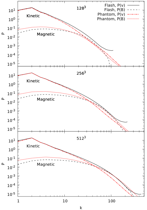
Figure 5.11: Time averaged kinetic and magnetic spectra in the saturated phase for Flash (black lines) and Phantom (red lines). As the resolution is increased, the magnetic energy spectra begins to overtake the kinetic energy spectra at high $k$ as found by Haugen et al. (2004).

Figure 5.11 compares the magnetic spectra to the kinetic energy spectra. It is characteristic for the small-scale dynamo for the peak in the magnetic energy spectrum to be at a wavenumber just above the peak in the kinetic energy spectrum (Cho and Vishniac, 2000; Brandenburg et al., 2012). This is clearly seen in Figure 5.11. The sharp peak at $k=2$ in the kinetic energy spectra is due to the driving force, and at all resolutions the peak of the magnetic energy spectra occurs just above this scale ($k\sim 3$–$4$).

The relative amount of energy in the magnetic field increases with resolution in both codes. For Phantom, the magnetic energy exceeds the kinetic energy at high $k$ at all three resolutions. For Flash, the magnetic energy spectra approaches the kinetic energy spectra with increasing resolution, overtaking it only in the $512^{3}$ calculation. Haugen et al. (2004) found that the magnetic energy spectra overtook the kinetic energy spectra at high $k$ in their ${\rm Pm}=1$ simulations, consistent with the Phantom results, though we note that the exact nature of this behaviour will certainly depend upon the magnetic Prandtl number.

5.3.3.4 PDFs of $B^{2}$

The red line in Figure 5.7 shows the time-averaged PDF of $B^{2}$ during the saturation phase, with the shaded region representing the standard deviation of the time-averaging. The distributions for Flash and Phantom peak at similar magnetic field strengths, agreeing to within 10% on the maximum of the peak, with similar ranges on the high-end tail of the distribution. The maximum magnetic field achievable agrees to within 10%. Similar to the growth phase, the low-end tail extends further for Flash, and has a larger standard deviation. From the linearly scaled plots of Figure 5.8, it is seen that the probability of being at the mean magnetic field strength increases by ${\sim}20\%$ once the magnetic field has saturated, corresponding to a reduced variance in the distribution of magnetic field strengths. This occurs due to the saturation of the strongest magnetic fields (Schekochihin et al., 2004b).

5.3.3.5 Density PDFs

Figure 5.12 compares the PDFs of the density contrast, $s\equiv\ln(\rho/\rho_{0})$ (for a motivation of this choice of variable, see Vazquez-Semadeni 1994; Federrath et al. 2008), during the growth phase, while the magnetic field is dynamically weak, to the saturation phase when the magnetic field is at its strongest. The PDFs in the growth phase were time-averaged during the first half of the growth phase while $E_{\rm m}<10^{-4}$ (excluding the initial transient growth). This allows for statistical averaging of a number of crossing times while the magnetic field is still dynamically weak. The PDFs in the saturation phase were averaged over at least $50t_{\rm c}$. The standard deviation from the time averaging is shown for the highest resolution calculations by the shaded regions (black for Flash, red for Phantom).

It has been noted many times that, for supersonic turbulence, the PDF of $s$ follows a log-normal distribution (e.g., Vazquez-Semadeni, 1994; Padoan et al., 1997; Passot and Vázquez-Semadeni, 1998; Nordlund and Padoan, 1999; Klessen, 2000; Lemaster and Stone, 2008; Federrath et al., 2008, 2010; Price and Federrath, 2010a; Federrath and Klessen, 2013). This is a consequence of the density at a location being perturbed randomly and independently over time. According to the central limit theorem, the PDF will converge to a log-normal distribution (Papoulis, 1984; Vazquez-Semadeni, 1994). Other processes may affect the shape of the PDF. Self-gravity has been demonstrated to add power-law tails at high densities (e.g., Klessen, 2000; Li et al., 2003; Federrath and Klessen, 2012), magnetic fields can narrow the width of the distribution effectively decreasing the compressibility of the gas (Collins et al., 2012; Molina et al., 2012; Federrath and Klessen, 2013), non-isothermal equations of state can introduce power-law tails at high and low densities (Passot and Vázquez-Semadeni, 1998; Li et al., 2003), and different forcing mechanisms (compressive vs solenoidal) influence the shape of the distribution (Federrath et al., 2008, 2010).

Both codes show PDFs close to a log-normal distribution in both the growth and saturation phases. As expected, Flash can be seen to sample a lower range of densities, while Phantom samples a higher range. This behaviour is similar to that found by PF10, and occurs because Phantom uses adaptive resolution based on the density. The stronger magnetic field in the saturation phase reduces the low-end tail of the distribution, making it more log-normally distributed, consistent with previous findings (Kowal et al., 2007; Lemaster and Stone, 2008; Price et al., 2011; Molina et al., 2012; Federrath and Klessen, 2013). The peak and high-end tail of the distribution remain quite similar during both the growth and saturation phases. Figure 5.13 shows the PDFs of $s$ on a linear scale. As before, the extended low-end tail for Flash is visible, but from this it is also clear that the mean of the distribution is higher for Phantom. This was also noted by PF10.

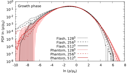
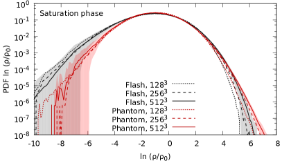
Figure 5.12: Time averaged density PDFs during the growth phase (top panel, for $t/t_{\rm c}=2$–$10$) and during the saturation phase (bottom panel, for $t/t_{\rm c}=30$–$100$, only $t\geq 50$ for the $128^{3}$ Phantom calculation). The peaks and high end tail of the PDF are similar for both cases, but the low density tail is less extended when the magnetic field has reached saturation.

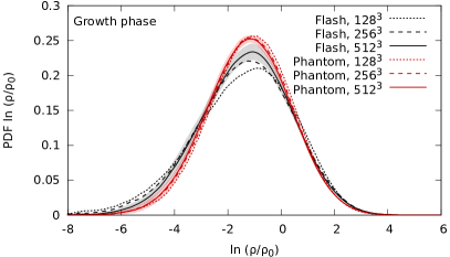
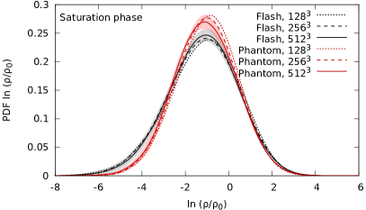
Figure 5.13: Time averaged density PDFs during the growth phase (top panel, for $t/t_{\rm c}=2$–$20$) and during the saturation phase (bottom panel, for $t/t_{\rm c}=30$–$100$, only $t/t_{\rm c}\geq 50$ for the $128^{3}$ Phantom calculation). This is equivalent to Figure 5.12 but on a linearly scaled plot. The peaks and high end tail of the PDF are similar for both cases, but the low density tail is less extended when the magnetic field has reached saturation.

5.4 Conclusions

We have performed a comparison between grid-based (Flash) and particle-based (Phantom) MHD methods on the small-scale dynamo amplification of magnetic fields. The calculations used supersonic turbulence driven at rms Mach 10 in an isothermal fluid contained in a periodic box. The initial magnetic field was uniform and had an energy $12$ orders of magnitude smaller than the mean kinetic energy.

Our conclusions are as follows:

i) Both codes exhibited similar qualitative behaviour. The initially weak magnetic field was exponentially amplified at a steady rate over a period of tens of turbulent crossing times, saturating when the magnetic energy was $2$–$4$% of the kinetic energy.

ii) The growth rate of magnetic energy in the Flash calculations varies only slightly with resolution (5–10%), while the Phantom calculations are sensitive to resolution (nearly doubling with each factor of two increase in resolution). This is due to the resolution scaling of the artificial dissipation terms.

iii) For ${\rm Pm}\sim 1$, the saturation level of magnetic energy appears to primarily depend on the magnetic Reynolds number, with little variation as the magnetic Prandtl number varies.

iv) Although Phantom is more computationally expensive, with the $256^{3}$ Phantom calculation taking as many cpu-hours as the $512^{3}$ Flash calculation, our results indicate the mean magnetic energy at saturation is comparable to Flash calculations at higher resolution.

v) Both codes show magnetic energy spectra at saturation that is relatively flat at large-scale, peaking around $k\sim 3$–$5$.

vi) During the growth phase, both codes produce a log-normal PDF of $B^{2}$ which linearly translates to higher magnetic field strengths over time.

vii) During the saturation phase, the PDF of $B^{2}$ in both codes becomes skewed, sampling a smaller range of magnetic field strengths.

This comparison has shown that SPMHD is capable of simulating the small-scale dynamo amplification of magnetic fields. We have performed this comparison using the ideal MHD equations, as many astrophysical simulations are performed under the assumption of ideal MHD. The most pressing follow-up to this work would be to perform a comparison using fixed physical dissipation terms in order to obtain agreement on the physical scaling of the growth rates.

Chapter 6 Conclusion

In this thesis, methods have been developed to improve the representation of magnetic fields in smoothed particle magnetohydrodynamics (SPMHD). The ideal MHD equations can be straightforwardly added to SPH with naive simplicity, however the resulting algorithm has numerical difficulties in simulating real astrophysical applications. The difficulty stems from the divergence-free constraint of the magnetic field. Maxwell’s equations cleanly state $\nabla\cdot{\bf B}=0$, but the induction equation, which describes the evolution of a magnetic field, does not manifestly enforce this.

6.1 Summary

6.1.1 Chapter 2 — Smoothed particle magnetohydrodynamics

Chapter 2 provided an overview of SPMHD. Insight into the numerical challenges surrounding $\nabla\cdot{\bf B}$ was obtained by deriving the ideal MHD equations in the continuum limit from the Euler fluid equations, Maxwell’s equations, and the Lorentz force law. Developing the discretisation of these equations into SPMHD started with the density estimate and variable smoothing length formulation. Using basic interpolation theory, the discretised version of the induction, energy, and momentum equations were obtained. Through understanding of the continuum equations, the instability present in the momentum equations was understood as arising from the inclusion of a term proportional to $\nabla\cdot{\bf B}$. Strategies to address this instability were presented. Methods for capturing shocks and discontinuities were also discussed.

6.1.2 Chapter 3 — Constrained hyperbolic divergence cleaning

In Chapter 3, we developed a constrained implementation of mixed hyperbolic/parabolic divergence cleaning based on the Dedner et al. (2002) method (see also Tricco and Price, 2012a). The premise is to couple a scalar field, $\psi$, to the magnetic field via a set of hyperbolic equations. These are used to propagate divergence through the magnetic field as a series of waves, with a parabolic diffusion term removing divergence error from the magnetic field. The hyperbolic waves make the parabolic diffusion more effective, as it increases the volume on which it can act.

In developing the numerical implementation of the cleaning system, it was useful to consider the physical picture of how it operates. Energy is transferred from the magnetic field into the $\psi$ field, then transported to a different location in a wavelike manner. It is key that energy be conserved in this process, otherwise, the waves might contain more energy than they did initially, leading to an increase in divergence error. This behaviour was indeed found by Price and Monaghan (2005) in their implementation. One circumstance where this may occur is at sharp density contrasts, where it can lead to a catastrophic increase in energy (see shocktube test 1B in Stasyszyn et al. 2013; also Section 3.4.2). Stasyszyn et al. (2013) used an artificial limiter to restrict the cleaning scheme in an attempt to reduce the severity of this error, but this does not address the fundamental issue of spurious energy production and reduces the overall effectiveness of the scheme.

Our method is ‘constrained’ in that it manifestly conserves the energy in the hyperbolic system of equations, inherently preventing spurious increases in the divergence of the magnetic field (consider again shocktube test 1B using our method in Section 4.2.1 and in Tricco and Price, 2013b). This was accomplished by defining the energy content of the $\psi$ field, then including it in the system Lagrangian. This allowed the discretised version of the hyperbolic equations to be obtained in the same manner as the SPMHD equations of motion — yielding versions which are guaranteed to conserve energy and to always decrease divergence error. This implementation was found to significantly increase the stability and robustness of the method, in particular solving issues with sharp density contrasts and free boundaries. This divergence cleaning scheme was found to yield an order of magnitude reduction of average divergence error on most test problems and astrophysical applications, and was responsible for the successful simulation of jets during the first hydrostatic core phase of star formation (Price et al. 2012, see also Tricco et al. 2013b; Bate et al. 2014a), and outflows during stellar core formation (Bate et al. 2014b, see also Price et al. 2013).

Enhancing the effectiveness of the divergence cleaning method was tested in two ways. One, by explicitly increasing the hyperbolic wave speed, with a corresponding reduction in timestep (over-cleaning). Two, by iterating the cleaning equations in-between timesteps (sub-cycling). We found that both approaches yield similar reductions in divergence error for the same number of steps (i.e., a factor of 10 increase in wave speed yields results similar to 10 iterations of sub-cycling the cleaning equations). Using sub-cycling, the divergence of the magnetic field may be set arbitrarily low provided a sufficient number of iterations are taken.

A formulation of the constrained hyperbolic divergence cleaning method was developed for the velocity field, for use in weakly compressible SPH simulations (see also Tricco and Price, 2012b). The aim is to improve the representation of incompressibility. Tests on an oscillating water drop reduced the magnitude of density variations by half, with negligible kinetic energy dissipation.

6.1.3 Chapter 4 — A switch to reduce resistivity

In Chapter 4, a new switch was developed and tested that dynamically regulates the amount of artificial resistivity applied to the magnetic field (see also Tricco and Price, 2013b). The motivation for a new switch arose during the course of a comparison of supersonic magnetised turbulence (Chapter 5). It was discovered that the PM05 switch completely failed to work for highly super-Alfvénic shocks. Therefore, a new switch was required which could detect discontinuities in the magnetic field regardless of the magnetic field strength. The new switch accomplished this by measuring the gradient of the magnetic field at the resolution scale normalised by the magnitude of the magnetic field. This measures the relative size of the jump in magnetic field strength, allowing it to detect discontinuities regardless of the absolute magnetic field strength.

This switch not only solved problems in detecting shocks in very weak magnetic fields, but was found to out-perform the PM05 switch in every respect. It reduced the L1 error by $7$–$45\%$ in a number of shocktube tests (containing a variety of magnetic shock types) compared to the PM05 switch. It resulted in lower magnetic energy dissipation in simulations of a circularly polarised Alfvén wave and the Orszag-Tang vortex problem. We concluded that it should be adopted for general use in SPMHD simulations.

The concept of the switch — using a normalised shock indicator — was used to construct switches for artificial viscosity and thermal conductivity (see also Tricco and Price, 2013a). The new artificial viscosity switch required a slow decay of $\alpha$ in order to treat post-shock oscillations, and was found to reproduce correct shock profiles in the Sod shocktube test.

6.1.4 Chapter 5 — Turbulent dynamo amplification of magnetic fields

In Chapter 5, we compared SPMHD (using the code Phantom) with grid-based methods (Flash) on the simulation of the turbulent small-scale dynamo amplification of a magnetic field (see also Tricco et al. 2014, and some early work which appeared in Tricco et al. 2013a, b). The turbulent motions on the smallest length scale efficiently twist and wind the magnetic field, imparting kinetic energy from the motion of the fluid into magnetic energy. The magnetic field as a whole grows through a reverse cascade, with energy being transported from small into large scales. This dynamo is an example of a fast dynamo, in that it leads to exponential amplification of the magnetic field. Since the dynamo operates near the smallest scales in the system, its growth rate is set by the combination of kinetic and resistive dissipation (kinetic and magnetic Reynolds numbers, and the ratio of the two, the magnetic Prandtl number). Once the magnetic field saturates on small scales, it enters a linear or quadratic growth phase as the reverse cascade continues to amplify large scales. The magnetic field fully saturates once the conversion of kinetic energy to magnetic energy is balanced by the dissipation of energy.

The simulations used supersonic turbulence to drive the dynamo. The conditions were representative of the interior of molecular clouds — the gas was isothermal, and had root mean square velocity of Mach 10. The turbulence was sustained through a stochastic driving force, with the pattern pre-generated so that both codes followed the same pattern as closely as possible. The initial conditions — uniform density, zero velocity, and a uniform magnetic field — were simple for the same reason. The simulations used a box of unit length with periodic boundary conditions, and were performed at three resolutions: $128^{3}$, $256^{3}$, and $512^{3}$.

Both methods had similar qualitative behaviour, with the magnetic energy being steadily amplified at an exponential rate until saturation. The saturation level of the mean magnetic energy was consistent at around $2$–$4\%$ of the mean kinetic energy, increasing with higher magnetic Reynolds numbers (i.e., higher resolution), though the saturation energy in the Phantom calculations was approximately equal to the Flash calculations at double the resolution.

The spectra of the magnetic energy had similar shape between the two methods, showing a relatively flat spectrum at low wavenumbers ($k<10$). In all calculations, the dynamo saturated the magnetic energy at smallest scales first. This marked the onset of the linear growth phase, during which the reverse cascade of magnetic energy slowly saturated the large scales. The saturated level of magnetic energy was similar at medium and small scales between the methods, though with the Phantom calculations containing twice as much magnetic energy at large scales ($k<10$) compared to Flash.

The rate of magnetic energy amplification differed between the two methods. For Flash, similar growth rates were obtained for the three resolutions simulated (within 5–10% difference). However, Phantom showed a stronger resolution dependence, with the growth rate nearly doubling with each factor of two increase in resolution. This effect was determined to be caused by the artificial viscosity and resistivity. Changing the dimensionless parameters in the dissipation terms ($\alpha$ and $\alpha_{\rm B}$) lead to the same effect as changing the resolution.

The probability distribution function (PDF) of magnetic field strengths was log-normal during the amplification phase. Its width remained constant, with the mean smoothly translating to higher field strengths over time. As the magnetic field approached saturation, the dynamo was unable to continue amplifying the strongest regions of the fields and the high-end tail of the distribution anchored in place. However, the low-end tail continued to increase, leading to a skewed distribution as the high-end tail became ‘squeezed’. Both methods exhibited this behaviour, agreeing to within 10% on the width and peak of the distributions, and on the location of the ‘anchor’ point of the high-end tail.

6.2 Future work

The direct extension to this thesis would be to continue developing the algorithms of SPMHD. The need for continued development will be best determined through application of the current methods to astrophysical problems. While the methods developed here have given a path forward on many problems, stress testing them through application will illuminate any weaknesses that need be addressed.

There are several aspects of the method that could be thought about further. The tensile instability in the equations of motion is understood as arising from the term proportional to $\nabla\cdot{\bf B}$ in the continuum equations. Subtracting this term solves the instability, and is attractive for its simplicity and physical motivation, though creates equations of motions which do not conserve momentum. It is not clear how to improve upon this aside from employing better methods to uphold the divergence-free constraint on the magnetic field.

In addition, the shock capturing methods used in SPMHD are rather crude in comparison to grid-based methods. As such, the numerical dissipation in SPMHD is typically higher than ‘standard’ grid-based methods. One issue is that artificial resistivity uses the fast MHD wave speed for the capture of all shock types, introducing a level of dissipation in excess of what is required for pure Alfvén waves. Iwasaki and Inutsuka (2011) developed a Godunov style shock solver for SPMHD that yields lower dissipation, and it would be interesting to investigate such approaches further.

The resolution of the magnetic field is tied to the mass. This is typically not a problem, as for the majority of astrophysical systems the regions of high mass are the most relevant. However consider the case of a neutron star. The magnetic field outside the neutron star is important, yet the density contrast at the surface is so large that the resolution of the magnetic field outside will be essentially absent if using equal mass particles. Also, consider the case of an accretion disc. SPH can simulate free boundaries easily, however, if the magnetic field is vertically aligned, then the field lines on the top and bottom boundaries of the disc are unphysically cut.

The immediate research plans for the future are for the following investigations:

6.2.1 Exactly upholding $\nabla\cdot{\bf B}=0$

The first is to find a suitable method to exactly maintain the divergence-free constraint of the magnetic field. The constrained hyperbolic divergence cleaning method only approximately upholds the divergence-free constraint, and it would be better to exactly maintain it. The Euler potentials and vector potential approaches have been already investigated as possible solutions, but neither are tenable in practice, and it is not clear how to adapt constrained transport to a particle method. Revisiting projection methods offer the best hope. PM05 have already developed scalar and vector projection methods, and testing these further would be of considerable interest. The difficulty is the computational cost involved, which only becomes trickier when dealing with individual timesteps.

Figure 6.1: Snapshots of $B_{\phi}$ at $t=1$, $20$, and $25\Omega$ for the $512^{2}$ 2D shearing box MRI test. Random small motions in the velocity lead to perturbations in the magnetic field ($t=1\Omega$). These coalesce to form large structures ($t=20\Omega$), which lead to the generation of turbulence ($t=25\Omega$). Renderings are not all on the same scale.

6.2.2 Magneto-rotational instability

The second research plan is to investigate SPMHD’s ability to simulate the magneto-rotational instability (MRI). A significant amount of work has been performed with grid-based methods on local simulations of accretion discs using the shearing box approximation. However, this has been shown to be deficient in capturing the global physics of accretion discs (e.g., Fromang and Papaloizou, 2007; King et al., 2007; Parkin and Bicknell, 2013). Due to its excellent angular momentum conservation and ability to simulate complex geometries and free boundaries, SPH is quite natural for simulating global accretion discs. Demonstrating that SPMHD can simulate the MRI would open a wide range of physical problems for future study.

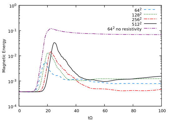
Figure 6.2: The evolution of magnetic energy for the 2D shearing box test. After several orbits, the stretching of the magnetic field lines triggers the MRI leading to exponential growth of magnetic energy.

Preliminary work has been performed on simulating the MRI in SPMHD. Vanaverbeke et al. (2014) used simulations of the MRI to test their SPMHD code, finding their results to have qualitative agreement with the grid-based simulations of Guan and Gammie (2008). In the following, we describe the results of simulations of the MRI in 2D shearing boxes. The initial density is uniform $\rho=1$. The equation of state is isothermal. The initial magnetic field is a sine wave in the $z$-direction, with amplitude defined to have plasma beta $\beta=1348$ ($B_{z}\approx 0.0358$). Random perturbations are introduced to the velocity field on the scale of $0.01~{}c_{\rm s}$. We note that these simulations use the quintic spline kernel in order to adequately resolve these small perturbations. These conditions mimic the fiducial model of Guan and Gammie (2008) and model S1 of Hawley and Balbus (1992). We perform the simulations for $100$ orbital periods ($t=100\Omega$ where $\Omega$ is the orbital frequency) at resolutions of $64^{2}$, $128^{2}$, $256^{2}$, and $512^{2}$. Since the flow is subsonic, we used the averaged Alfvén speed in the artificial resistivity signal velocity, rather than the fast MHD wave speed. We found that at low resolutions, the dissipation from using the fast MHD wave speed can prevent the instability from activating. Similarly, Vanaverbeke et al. (2014) comment that they use only the $\nabla\cdot{\bf B}$ source term when using the PM05 switch in order to avoid excessive dissipation.

Snapshots of the $\phi$ component of the magnetic field at $t=1$, $20$, and $25\Omega$ are presented in Figure 6.1. The correct qualitative behaviour is obtained: random motions in the initial conditions induce small perturbations in the magnetic field, which coalesce leading to turbulent motion. The magnetic energy as a function of time is given by Figure 6.2. The MRI leads to an exponential increase in magnetic energy which decays once turbulence has formed. The location of the peak is in agreement with Guan and Gammie (2008). It occurs later for higher resolutions because the energy contained in the perturbations is at smaller scales, requiring more time for the perturbations to coalesce into large structures. The maximum magnetic energy achieved increases with resolution due to the reduction in numerical dissipation. Notably, the decay in magnetic energy is more rapid than in the grid-based results. This is due to the level of magnetic energy dissipation. The switch developed in Chapter 4 will activate when the field undergoes reversals in direction (${\bf B}\to 0$), which is the correct behaviour at current sheets, but adds an unnecessary level of dissipation for this problem. We have performed a $64^{2}$ resolution calculation with no artificial resistivity applied, the results of which are included in Figure 6.2. The maximum energy level achieved is over an order of magnitude higher than the same resolution with artificial resistivity, with only a slow decay in magnetic energy after. This preliminary work shows promise that SPMHD can activate the MRI, though further work is needed.

6.3 Conclusion

The methods developed in this thesis have significantly advanced SPMHD as a numerical method capable of performing astrophysical MHD simulation. The proof is in the pudding: they have already lead to published work on the role of magnetic fields in the formation of protostars (Price et al., 2012; Bate et al., 2014b). To quote Price and Monaghan (2005),

Our results suggest that the method is ripe for application to problems of current theoretical interest, such as that of star formation.

Appendix A Artificial $\psi$-dissipation term

Although the hyperbolic divergence cleaning method developed in Chapter 3 already includes a damping term to reduce $\psi$, we have investigated the addition of a new dissipation term, analogous to artificial resistivity or viscosity, of the form

$$\left(\frac{{\rm d}\psi_{a}}{{\rm d}t}\right)_{\text{diss}}=\rho_{a}\sum_{b}m_{b}\frac{c_{\rm h}\alpha_{\psi}}{\overline{\rho}_{ab}^{2}}\left(\psi_{a}-\psi_{b}\right)F_{ab},$$ (A.1)

where $\nabla W_{ab}=\hat{\bf r}_{ab}F_{ab}$. This dissipation term is mainly designed to capture discontinuities in the $\psi$ field, motivated by our neglect of the surface integral term in Equation 3.9. The term is essentially an SPH expression for a diffusion term of the form $\eta_{\psi}\nabla^{2}\psi$, where $\eta_{\psi}\propto\alpha_{\psi}c_{\rm h}h$, which in comparison to the damping term, acts more strongly to smooth relative differences in $\psi$. This artificial $\psi$-dissipation can be used in conjunction with the damping term, however since both the damping and diffusion terms dissipate $\psi$, it is important that values of $\alpha_{\psi}$ and $\sigma_{\psi}$ be chosen carefully to avoid overdamping the system. For example, we found that in our two dimensional tests that propagation of divergence waves were damped too severely with $\alpha_{\psi}=1$, and that using $\alpha_{\psi},\sigma_{\psi}=[0.1,0.2]$ or $[0.2,0.1]$ yielded near critical damping (see Figure A.1).

For this dissipation term, the energy loss is given by

$$\sum_{a}m_{a}\frac{\psi_{a}}{\mu_{0}\rho_{a}c_{\rm h}^{2}}\left(\frac{{\rm d}\psi_{a}}{{\rm d}t}\right)_{\text{diss}}=\sum_{a}m_{a}\frac{\psi_{a}}{\mu_{0}c_{\rm h}}\sum_{b}m_{b}\frac{\alpha_{\psi}}{\overline{\rho}_{ab}^{2}}\left(\psi_{a}-\psi_{b}\right)F_{ab}.$$ (A.2)

This can be shown to be negative definite by splitting the RHS into two halves, performing a change of summation indices on the second half, then rejoining to obtain

$$-\frac{1}{2}\sum_{a}m_{a}\frac{\alpha_{\psi}}{\mu_{0}c_{\rm h}}\sum_{b}m_{b}\frac{\left(\psi_{a}-\psi_{b}\right)^{2}}{\overline{\rho}_{ab}^{2}}F_{ab},$$ (A.3)

which, since $F_{ab}$ is negative for positive kernels, gives a negative definite contribution to the total energy (and conversely would give a positive definite heat contribution).

Inclusion of the dissipation term was tried with all test cases presented in Section 3.4. Similar reductions in the divergence error were obtained, however no results were improved beyond that of using the damping alone (Fig. A.1).

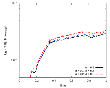
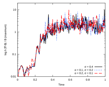
Figure A.1: Average and maximum divergence error when including the new, artificial $\psi$ dissipation term in the Orszag-Tang vortex test. Values of $\alpha_{\psi}$ and $\sigma_{\psi}$ are chosen so that the combination is close to critical damping, however no benefit is noted over use of the regular damping term.

Appendix B Interpolating particle data to a grid

The power spectra of kinetic and magnetic energy of the Phantom calculations (Chapter 5) are computed by interpolating the particle data to a grid using an SPH kernel weighted summation over neighbouring particles. We have investigated whether using mass weighted or volume weighted interpolation changes the results. Furthermore, we have tested grids of varying resolution to find the optimal grid resolution to properly represent the magnetic field.

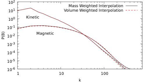
Figure B.1: Time averaged kinetic and magnetic spectra of the $256^{3}$ particle Phantom calculation interpolated to a grid using mass weighted and volume weighted interpolation. Both approaches yield the same result.

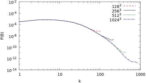
Figure B.2: Conversion of a $128^{3}$ particle Phantom snapshot to grids of resolutions from $128^{3}$ to $1024^{3}$ grid points. Each resolution agrees well on the large-scale structure, but captures more of the small-scale structure as the resolution is increased. We find that the $256^{3}$ sufficiently the total magnetic energy, therefore choose grids with double the number the grid points as particles for our analysis.

The volume weighted interpolation of a quantity $A$ (in this case, the magnetic field ${\bf B}$) may be computed according to

$${\bf B}({\bf r})=\frac{\sum_{b}\dfrac{m_{b}}{\rho_{b}}{\bf B}_{b}W(|{\bf r}-{\bf r}_{b}|,h_{b})}{\sum_{c}\dfrac{m_{c}}{\rho_{c}}W(|{\bf r}-{\bf r}_{c}|,h_{c})}.$$ (B.1)

The denominator is the normalisation condition. A mass weighted interpolation may be computed as

$${\bf B}({\bf r})=\frac{\sum_{b}m_{b}{\bf B}_{b}W(|{\bf r}-{\bf r}_{b}|,h_{b})}{\sum_{c}m_{c}W(|{\bf r}-{\bf r}_{c}|,h_{c})}.$$ (B.2)

Figure B.1 shows the kinetic and magnetic energy spectra for the $128^{3}$ Phantom calculation computed from a grid using volume weighted and mass weighted interpolations, respectively. The spectra between the two interpolation methods are nearly indistinguishable, differing from each other by less than 1% at all $k$ and deviating only near the resolution scale. We conclude that either approach is acceptable, and for the spectra generated in Chapter 5, we have used the mass weighted interpolation.

The smoothing length in the calculations in Chapter 5 can decrease by up to $8\times$ in the highest density regions, therefore we have tested the effect of different grid resolutions on the magnetic spectra. Figure B.2 shows magnetic energy spectra from a $128^{3}$ particle Phantom calculation interpolated to grids with resolutions of $128^{3}$ to $1024^{3}$. Our results show that the large-scale structure ($k<50$) is nearly identical at all grid resolutions, with the spectra differing on the order of $0.1\%$ at each $k$-band. The only difference is that the spectra extends to higher $k$ as the resolution is increased. We find that the magnetic energy contained on the $128^{3}$ grid differs by $1\%$ of the energy contained on the particles, while the $256^{3}$ grid resolution differs by only $0.1\%$. Higher resolutions only minimally change the energy content of the magnetic field. Our conclusion is that a grid with double the resolution of the Phantom calculation is sufficient for computing the magnetic energy spectra accurately.

Appendix C Effective magnetic Prandtl numbers in grid and particle methods

C.1 Prandtl numbers in Eulerian schemes

The primary source of numerical dissipation in Eulerian schemes is from the discretisation of advection terms. Consider a simple example of the contents of one grid cell advecting into an adjacent grid cell. If only a partial amount is transferred into the adjacent cell, then the contents must be reconstructed from the flux across the boundary. This approximation introduces diffusion due to its truncation error (e.g., Robertson et al., 2010). The diffusion term in the first-order upwind scheme of Courant et al. (1952), for example, scales according to $\propto v\Delta x(1-|C|)$, where $C=v\Delta t/\Delta x$ is the Courant number. Higher order methods will change the scaling of the diffusion, but in all schemes it depends upon the resolution, time step size, and fluid velocity.

Quantifying the effective numerical dissipation may be done by comparing simulations against analytic solutions. Lesaffre and Balbus (2007) compared the analytic solution of a linear mode of the magneto-rotational instability (MRI) to shearing box simulations in order to calibrate their version of Zeus3D. They varied the size of the time step and investigated resolutions from $32^{3}$ to $128^{3}$, determining that the total numerical dissipation (viscous and resistive) scaled linearly with time and quadratically with resolution. They found the magnetic Prandtl number to be approximately 2 (though in the context of this comparison, these simulations are for subsonic flows). In a similar manner, Fromang et al. (2007) performed simulations of the MRI with and without physical viscous and resistive dissipation terms. They found that the results of their ideal MHD simulations (dissipation is purely numerical) corresponded to ${\rm Pm}\approx 2$, though cautioned that this depends upon the nature of the flow.

The effective Prandtl number for the version of Flash used in Chapter 5 was calibrated by Federrath et al. (2011). Using simulations of the small-scale dynamo amplification of a magnetic field, they compared results from ideal MHD simulations to simulations employing a fixed dissipation (at varying resolution). They found that ${\rm Pm}\approx 2$ for flows of Mach numbers $0.4$ and $2$. Thus, it is expected that the Flash calculations in our comparison will have a similar Prandtl number.

C.2 Prandtl numbers in smoothed particle magnetohydrodynamics

In SPMHD, the equations of motion are derived from the discretised Lagrangian (Price and Monaghan, 2004b; Price, 2012). Advection is computed exactly. Hence, the only sources of numerical dissipation are from the explicit sources of artificial viscosity and resistivity, which can be used to estimate the Reynolds and Prandtl numbers.

Artificial viscosity and resistivity in SPMHD are discretisations of physical dissipation terms, but with diffusion parameters that depend on resolution. Artymowicz and Lubow (1994) and Murray (1996) analytically derived the amount of corresponding physical dissipation from the Monaghan and Gingold (1983) form of artificial viscosity (see also Monaghan 2005; Lodato and Price 2010). The artificial viscosity acts as both a shear and bulk viscosity. In these calculations, we use the Monaghan (1997) form of artificial viscosity, which is similar except for the absence of a factor $h/|r_{ab}|$. Meru and Bate (2012) calculated the amount of viscosity this adds in the continuum limit, and have shown that for the Monaghan (1997) form of viscosity, it is approximately 18% stronger for the $\alpha$ term. Using this approach, they also derived the coefficients for the $\beta_{\rm AV}$ term in the signal velocity. Hence, the shear viscosity in the simulations in Chapter 5 corresponds to

$$\nu_{\rm AV}=\frac{62}{525}\alpha v_{\rm sig}h+\frac{9}{35\pi}\beta_{\rm AV}|\nabla\cdot{\bf v}|h^{2}.$$ (C.1)

where

$$v_{\rm sig}=\sqrt{c_{\rm s}^{2}+v_{\rm A}^{2}}.$$ (C.2)

The bulk viscosity will be $5/3\times$ this value (Lodato and Price, 2010).

We note that these coefficients are twice the values quoted by Meru and Bate (2012). Their work is derived in the context of a Keplerian accretion disc, in which they safely assume that half the particles inside a particle volume are approaching while the other half are receding. It is standard in SPH to apply artificial viscosity only to approaching particles. In this paper, we calculate Reynolds numbers for particles where $\nabla~{}\cdot~{}{\bf v}~{}<~{}0$, and use the full value of the coefficient as it is expected that inside a shock, nearly all particles will be approaching. The bulk viscosity will be important for supersonic flows, which will affect the Reynolds number. In order to compare Reynolds numbers with Flash, we compute the Reynolds numbers using only the shear viscosity. Including this term in the estimate of the Reynolds number would lead to larger ${\rm Pm}$ values.

The corresponding physical dissipation from the artificial resistivity can be calculated in a similar manner (Section 2.2.10.2). Artificial resistivity corresponds to a physical resistivity given by

$$\eta_{\rm AR}=\frac{1}{2}\alpha_{\rm B}v_{\rm sig}h.$$ (C.3)

We note, as concluded in Chapter 4, that the $\beta_{\rm AV}$ term in the artificial viscosity is not required for artificial resistivity. It is added to artificial viscosity to prevent particle interpenetration in high Mach number shocks, and otherwise leads to unnecessary dissipation if added to artificial resistivity.

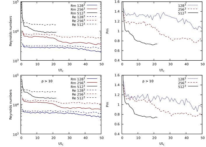
Figure C.1: The kinetic and magnetic Reynolds numbers (left plots) and Prandtl numbers (right plots) for Phantom. The top row shows the averaged numbers for particles which have $\nabla\cdot{\bf v}<0$, while the bottom row is averaged for regions where $\rho>10\rho_{0}$. The higher density regions have approximately double the kinetic and magnetic Reynolds numbers. The drop in Reynolds and Prandtl numbers over time is due to the fast MHD wave speed increasing in the signal velocity of the artificial dissipation terms. The Prandtl numbers are about unity, though decrease with resolution.

Since the dissipation terms use the local signal velocity, and our simulations use switches to dynamically adjust the values of $\alpha$ and $\alpha_{\rm B}$ for each particle, $\nu_{\rm AV}$ and $\eta_{\rm AR}$ are calculated per particle. In Figure C.1, we show the average kinetic Reynolds, magnetic Reynolds, and magnetic Prandtl numbers on the particles for our simulations. We find that the mean Prandtl number in these set of SPMHD calculations is approximately unity. The Prandtl number decreases with resolution, a consequence of the quadratic scaling of the $\beta_{\rm AV}$ term, which is present in the artificial viscosity but not artificial resistivity. The Prandtl number also decreases with time. This results from the signal velocity scaling behaviour, as the dissipation from the $\alpha$ term increases as the magnetic field is amplified ($v_{\rm A}$ increasing). The $\beta_{\rm AV}$ term is unaffected by this. For high-density regions ($\rho>10$), we note that the Reynolds numbers are increased by approximately a factor of 2, directly corresponding to the reduction in $h$.

References

- Agertz et al. (2007) Agertz, O., B. Moore, J. Stadel, D. Potter, F. Miniati, J. Read, L. Mayer, A. Gawryszczak, A. Kravtsov, Å. Nordlund, F. Pearce, V. Quilis, D. Rudd, V. Springel, J. Stone, E. Tasker, R. Teyssier, J. Wadsley, and R. Walder: 2007, ‘Fundamental differences between SPH and grid methods’. MNRAS 380, 963–978.
- André et al. (2010) André, P., A. Men’shchikov, S. Bontemps, V. Könyves, F. Motte, N. Schneider, P. Didelon, V. Minier, P. Saraceno, D. Ward-Thompson, J. di Francesco, G. White, S. Molinari, L. Testi, A. Abergel, M. Griffin, T. Henning, P. Royer, B. Merín, R. Vavrek, M. Attard, D. Arzoumanian, C. D. Wilson, P. Ade, H. Aussel, J.-P. Baluteau, M. Benedettini, J.-P. Bernard, J. A. D. L. Blommaert, L. Cambrésy, P. Cox, A. di Giorgio, P. Hargrave, M. Hennemann, M. Huang, J. Kirk, O. Krause, R. Launhardt, S. Leeks, J. Le Pennec, J. Z. Li, P. G. Martin, A. Maury, G. Olofsson, A. Omont, N. Peretto, S. Pezzuto, T. Prusti, H. Roussel, D. Russeil, M. Sauvage, B. Sibthorpe, A. Sicilia-Aguilar, L. Spinoglio, C. Waelkens, A. Woodcraft, and A. Zavagno: 2010, ‘From filamentary clouds to prestellar cores to the stellar IMF: Initial highlights from the Herschel Gould Belt Survey’. A&A 518, L102.
- Artymowicz and Lubow (1994) Artymowicz, P. and S. H. Lubow: 1994, ‘Dynamics of binary-disk interaction. 1: Resonances and disk gap sizes’. ApJ 421, 651–667.
- Balbus and Hawley (1991) Balbus, S. A. and J. F. Hawley: 1991, ‘A powerful local shear instability in weakly magnetized disks. I - Linear analysis. II - Nonlinear evolution’. ApJ 376, 214–233.
- Balsara (1995) Balsara, D. S.: 1995, ‘von Neumann stability analysis of smooth particle hydrodynamics–suggestions for optimal algorithms’. J. Comput. Phys. 121, 357–372.
- Barnes et al. (2012) Barnes, D. J., D. Kawata, and K. Wu: 2012, ‘Cosmological simulations using GCMHD+’. MNRAS 420, 3195–3212.
- Batchelor (2000) Batchelor, G.: 2000, An Introduction to Fluid Dynamics, Cambridge Mathematical Library. Cambridge University Press.
- Bate et al. (1995) Bate, M. R., I. A. Bonnell, and N. M. Price: 1995, ‘Modelling accretion in protobinary systems’. MNRAS 277, 362–376.
- Bate et al. (2014a) Bate, M. R., D. J. Price, and T. S. Tricco: 2014a, ‘Modelling Magnetised Protostellar Jets with SPH’. In: D. Stamatellos, S. Goodwin, and D. Ward-Thompson (eds.): The Labyrinth of Star Formation, Vol. 36 of Astrophysics and Space Science Proceedings. Springer International Publishing, pp. 101–104.
- Bate et al. (2014b) Bate, M. R., T. S. Tricco, and D. J. Price: 2014b, ‘Collapse of a molecular cloud core to stellar densities: stellar-core and outflow formation in radiation magnetohydrodynamic simulations’. MNRAS 437, 77–95.
- Beck et al. (2013) Beck, A. M., K. Dolag, H. Lesch, and P. P. Kronberg: 2013, ‘Strong magnetic fields and large rotation measures in protogalaxies from supernova seeding’. MNRAS 435, 3575–3586.
- Beck et al. (2012) Beck, A. M., H. Lesch, K. Dolag, H. Kotarba, A. Geng, and F. A. Stasyszyn: 2012, ‘Origin of strong magnetic fields in Milky Way-like galactic haloes’. MNRAS 422, 2152–2163.
- Bellan (2006) Bellan, P.: 2006, Fundamentals of Plasma Physics. Cambridge University Press.
- Benz et al. (1990) Benz, W., A. G. W. Cameron, W. H. Press, and R. L. Bowers: 1990, ‘Dynamic mass exchange in doubly degenerate binaries. I - 0.9 and 1.2 solar mass stars’. ApJ 348, 647–667.
- Berger and Colella (1989) Berger, M. J. and P. Colella: 1989, ‘Local adaptive mesh refinement for shock hydrodynamics’. J. Comput. Phys. 82, 64–84.
- Biermann (1950) Biermann, L.: 1950, ‘Über den Ursprung der Magnetfelder auf Sternen und im interstellaren Raum (miteinem Anhang von A. Schlüter)’. Zeitschrift Naturforschung Teil A 5, 65.
- Blandford and Payne (1982) Blandford, R. D. and D. G. Payne: 1982, ‘Hydromagnetic flows from accretion discs and the production of radio jets’. MNRAS 199, 883–903.
- Bonafede et al. (2011) Bonafede, A., K. Dolag, F. Stasyszyn, G. Murante, and S. Borgani: 2011, ‘A non-ideal magnetohydrodynamic GADGET: simulating massive galaxy clusters’. MNRAS 418, 2234–2250.
- Bonet and Lok (1999) Bonet, J. and T.-S. L. Lok: 1999, ‘Variational and momentum preservation aspects of smooth particle hydrodynamic formulations’. Comput. Methods Appl. Mech. Eng. 180(1-2), 97–115.
- Børve et al. (2001) Børve, S., M. Omang, and J. Trulsen: 2001, ‘Regularized Smoothed Particle Hydrodynamics: A New Approach to Simulating Magnetohydrodynamic Shocks’. ApJ 561, 82–93.
- Børve et al. (2004) Børve, S., M. Omang, and J. Trulsen: 2004, ‘Two-dimensional MHD Smoothed Particle Hydrodynamics Stability Analysis’. ApJS 153, 447–462.
- Bourke et al. (2001) Bourke, T. L., P. C. Myers, G. Robinson, and A. R. Hyland: 2001, ‘New OH Zeeman Measurements of Magnetic Field Strengths in Molecular Clouds’. ApJ 554, 916–932.
- Bovino et al. (2013) Bovino, S., D. R. G. Schleicher, and J. Schober: 2013, ‘Turbulent magnetic field amplification from the smallest to the largest magnetic Prandtl numbers’. New J. Phys. 15(1), 013055.