A New Catalog of Variable Stars in the Field of the Open Cluster M37

Abstract

We present a comprehensive re-analysis of stellar photometric variability in the field of the open cluster M37 following the application of a new photometry and de-trending method to MMT/Megacam image archive. This new analysis allows a rare opportunity to explore photometric variability over a broad range of time-scales, from minutes to a month. The intent of this work is to examine the entire sample of over 30,000 objects for periodic, aperiodic, and sporadic behaviors in their light curves. We show a modified version of the fast $\chi^{2}$ periodogram algorithm (F$\chi^{2}$) and change-point analysis (CPA) as tools for detecting and assessing the significance of periodic and non-periodic variations. The benefits of our new photometry and analysis methods are evident. A total of 2306 stars exhibit convincing variations that are induced by flares, pulsations, eclipses, starspots, and unknown causes in some cases. This represents a 60% increase in the number of variables known in this field. Moreover, 30 of the previously identified variables are found to be false positives resulting from time-dependent systematic effects. New catalog includes 61 eclipsing binary systems, 92 multiperiodic variable stars, 132 aperiodic variables, and 436 flare stars, as well as several hundreds of rotating variables. Based on extended and improved catalog of variables, we investigate the basic properties (e.g., period, amplitude, type) of all variables. The catalog can be accessed through the web interface (http://stardb.yonsei.ac.kr/).

1 Introduction

The rich open cluster M37 (NGC 2099) in the constellation Auriga has been photometrically monitored to search for new variables with different motivations (Kiss et al., 2001; Kang et al., 2007; Messina et al., 2008; Hartman et al., 2008a). The combination of short and deep exposures with similar sky coverage allowed time-series photometry of hundreds to thousands of stars from the brightest to the dimmest within the cluster field ($10<V<23$). Their studies indicate that the fraction of variable sources $f_{\mathrm{var}}$ increases as photometric precision of the survey gets better.

Kiss et al. (2001) performed the first variability survey for the central ($29\arcmin\times 18\arcmin$) field of the M37 with a $R_{C}$-filter photometry and found 7 variable stars among 2300 stars ($f_{\mathrm{var}}\sim 0.3\%$). Due to poor photometric quality, their variables were with large variability and included three W UMa-type eclipsing binaries (EBs), two high-amplitude pulsating stars, and two long-period detached EB candidates.

Kang et al. (2007) and Messina et al. (2008) used the same data set to search for short-period pulsating variables (e.g., $\delta$ Scuti- and $\gamma$ Doradus-type stars) and rotating variables of later spectral types (F–K), respectively. Using $V$-band time-series observations, these two studies found the total of 153 variable stars among 12,000 stars ($f_{\mathrm{var}}\sim 1.3\%$), including seven previously known variables, in the field of the cluster ($22.2\arcmin\times 22.2\arcmin$).

Lastly, the most extensive variability studies in this field were carried out by Hartman et al. (2008b, 2009a, 2009b) as the by-products of a deep survey for transiting planets in the M37 field ($24\arcmin\times 24\arcmin$) with the 6.5m MMT telescope. The number of known variable stars increased by a factor of $\sim$10. By applying several statistical algorithms, they identified 1445 variables among 23,000 stars ($f_{\mathrm{var}}\sim 6.3\%$), of which 99% were new discoveries (Hartman et al., 2008b). This catalog of variable stars provides the largest homogeneous set of stellar rotation periods for a cluster older than 500 Myr, which showed the crucial role of the rotation in the stellar angular momentum evolution (Hartman et al., 2009a).

In this paper, we search new variable phenomena from the same data set of Hartman et al. (2008a) with vastly improved photometric method (Chang et al. 2015, hereafter Paper I). In Section 2, we give a brief description of new light curves and its temporal properties. We present a comprehensive re-analysis of photometric variability in Section 3. In Section 4, we present a new catalog of variable stars and various variability characteristics. We compare our findings with previous works and discuss the nature of each variability class separately in Section 5.

Figure 1: Observational cadence of the MMT transit survey, showing cumulative fraction function of time intervals $\Delta T_{\mathrm{mjd}}$ between two consecutive frames (top left) and the exposure times $T_{\mathrm{exp}}$ (top right). We use logarithmic scale for the horizontal axis in these two panels. The bottom panel is the distribution of exposure times as a function of the modified Julian date (MJD).

2 Data description

We refer the reader to Paper I for a detailed description of our photometric reduction and light curve production applied to the archival imaging data of MMT transit survey. Here we provide only a brief summary of the key features. In Paper I, we introduced new methods for robust high-precision photometry from well-sampled images of a non-crowded field with strongly varying PSF. The archival light curves from the original image subtraction procedure exhibit many unusual outliers, and more than 20% of data get rejected by the simple filtering algorithm adopted by early analysis. We note that some of these outliers are results of intrinsic variability of short time scales. In order to achieve better photometric precisions and also to utilize all available data, the entire imaging database were re-analyzed with our multi-aperture indexing photometry and a set of sophisticated calibration procedures. This algorithm finds an optimal aperture for each star with a maximum signal-to-noise ratio, and also treat peculiar situations where photometry returns misleading information with more optimal photometric index. We also applied photometric de-trending algorithm based on a hierarchical clustering method. Our method removes systematic variations that are shared by light curves of nearby stars while true variabilities are preserved. Consequently, our method utilizes nearly 100% of available data and reduce the RMS scatter several times smaller than original analysis for brighter stars.

Our new data set includes 30,294 objects, including both point and extended sources. For blended targets, the original image subtraction light curve is still of higher precision than the present aperture photometry light curves, and thus for these objects the archival light curve is used. In order to pick out such cases, we utilized a simple method for quantifying the level of blending (see Irwin et al. 2007).

$$b=\frac{\chi^{2}-\chi_{poly}^{2}}{\chi^{2}}$$

where

$$\chi^{2}=\sum_{p}\frac{(\sum m_{p}-\bar{m}_{j})^{2}}{\sigma_{p}^{2}}$$ (1)

for light curve points $m_{p}$ with uncertainties $\sigma_{p}$, and $\chi_{poly}^{2}$ is the same statistic measured with respect to a 4th order polynomial fit. We adopt the value $b>0.6$ for selecting significant blended light curves, and then count the number of blended ones (3746 objects).

Figure 1 shows that the cumulative fraction function of temporal intervals $\Delta T_{mjd}$ between two consecutive frames and the exposure times $T_{exp}$. This observing cadence is sensitive to variability on timescales ranging from tens of seconds (30 seconds) to one month ($\sim$31.7 days). In particular, the time resolution allows an analysis of the short-term variability, which is less than $\sim$80 seconds over 50% of the data and $\sim$150 seconds over 90% of the data.

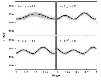
(a)

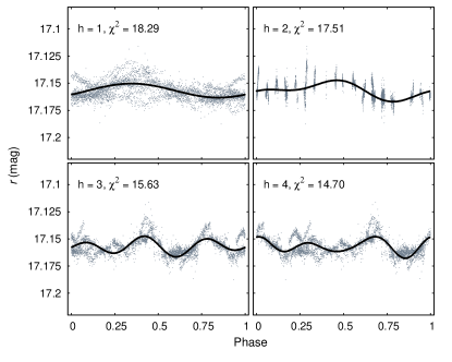
(b)

Figure 2: Example light curves of a periodic star (four plots at left panel) and another quasi-periodic star (four plots at right panel) with different periods detected by the first feature detection algorithm, respectively. The shape of periodic feature is varied widely by the selected harmonic model $h$ (from 1 to 4), but we can choose the best candidate with $\chi^{2}$ statistics.

3 Variability-analysis methods

Variability features can be divided into two broad categories: periodic and non-periodic feature. The former is easier to detect and model using statistical and model-specific fitting procedures as a form of Fourier series (e.g., Debosscher et al. 2007, 2009; Richards et al. 2011). But the latter is rather ambiguous, since it is not always possible to characterize flux variation and to define a reliable range for some parameters. To overcome this difficulty, Richards et al. (2011) calculated many basic statistics that can describe the distribution of fluxes even in the limit of few data points. One interesting approach is to select stochastically varying features in quasar-like sources. The correlated variability of quasars is well parameterized by a damped random walk model, providing a simple statistical description of their characteristic timescales and amplitudes (e.g., Kelly et al. 2009; Butler & Bloom 2011). In this work we use a modified version of the fast $\chi^{2}$ periodogram algorithm (F$\chi^{2}$) and the change-point analysis (CPA) method for detecting and assessing the significance of periodic and non-periodic signals, respectively.

3.1 Generic periodic feature detection

We first searched a periodic feature by F$\chi^{2}$ technique that calculates the minimized $\chi^{2}$ as a function of frequency at the desired number of harmonics (Palmer, 2009). With the best-fit frequency, we compared the ratio between the variance of the data after subtracting the best-fit model and full-amplitude of model function. This algorithm use a Fourier series truncated at harmonic $h$ as a model function:

$$\Phi_{h}=A_{0}+\sum_{h=1}^{\mathrm{4}}A_{2h-1}\sin(h2\pi ft)+A_{2h}\cos(h2\pi ft)$$ (2)

The fitting coefficients ($A_{0}$, $A_{2h}$, and $A_{2h-1}$) obtained in each harmonic model provide a reasonable description of a generic periodic feature, irrespective of the feature shape, as discussed by Debosscher et al. (2009). Figure 2 shows example light curves of both periodic (new variable star; V1983) and long-term (V1092) variable stars in our sample, respectively. Because the optimal choice of $h$ depends on the true shape of the signal, the fit quality is evaluated for each model with standard $\chi^{2}$ statistics, and then checked the residual (phase-folded) light curves after the subtraction of the best-fit model. To test the significance of a signal, we use the ratio between the full-amplitude of the model function ($\mathrm{Famp}$ = $m_{max}-m_{min}$) and the RMS scatter ($\sigma_{a}$) of the data after model subtraction:

$$\mathrm{Famp}\geq\lambda\sigma_{a}.$$ (3)

The lower limit for the ratio is empirically set to $\lambda$ = 0.95 based on light curve inspections. $\lambda$-values less than 0.95 indicate that we do not expect any significant (semi-) periodic signals for a given light curve. Even when the source is poorly described by the harmonic fit, this indicator provides a hint of a generic periodic signal (see right panel of Figure 2).

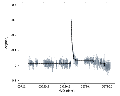
(a)

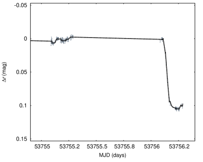
(b)

Figure 3: Example light curves of flare-like (left panel) and eclipsing-like (right panel) events detected by the second feature detection algorithm. We used the default values of the variable parameters ($N_{1}$=3, $N_{2}$=1, $N_{3}$=3) as the detection thresholds. The CPA model is over-plotted in dashed lines.

3.2 Arbitrary-shaped and sporadic event detection

3.2.1 Change-point analysis (CPA)

Most variability detection methods require conventional models that are mainly focused on the periodic signals, and are not suitable for the study of arbitrary-shaped, non-periodic, and sporadic variations. Also, in many cases, signal estimation is equated with smoothing of data for de-noising. This sometimes discards vital information in time series data. We introduce a non-parametric method to extract all significant features based on the CPA using local statistics.

Change-point analysis is a method to identify abrupt variations in sequential data. It is widely used in the statistics and data mining communities as well as in the field of time domain astronomy (see e.g., Schütz & Holschneider 2011 and reference therein). Using a combination of cumulative sum scheme (CUSUM) and bootstrap rank statistics (Taylor, 2000), we produce a series of estimated change-points which correspond to the moments of apparent systematic changes. For a given dataset {$x_{1}$, $x_{2}$, $\cdots$, $x_{n}$} of size $n$, the CUSUM values are given by

$$S_{t}=\sum_{i=1}^{t}(x_{i}-\bar{x})$$ (4)

for $t$ = $0,1,\cdots,n$, where $S_{0}$ = 0 and the mean value $\bar{x}$ for the sample of $n$ values of $x_{i}$. An inflection point at which the sign of the CUSUM slope changes is used to determine whether a given interval of data should be kept as one ($\bar{x}_{1}$=$\bar{x}_{2}$=$\cdots$=$\bar{x}_{n}$=$\bar{x}$) or subdivided into two subintervals ($\bar{x}_{1}$=$\cdots$=$\bar{x}_{p}$$\neq$$\bar{x}_{p+1}$=$\bar{x}_{n}$). Based on $N(\geq 1,000)$ bootstrap samples that are randomly re-ordered original values, we estimate the confidence level (c.l.) to reduce the false positives by random noise. Here are the main procedure of each bootstrap process:

• We generate a bootstrap sample of $n$ dataset, denoted {$x_{1}^{b}$, $x_{2}^{b}$, $\cdots$, $x_{n}^{b}$}, by randomly re-ordering the original $n$ values without replacement.

• Based on the bootstrap dataset, we calculate the bootstrap CUSUM $S_{t}^{b}$ by using equation (4), and then obtain the maximum, minimum, and difference of the bootstrap CUSUM.

  $$S_{diff}^{b}=S_{max}^{b}-S_{min}^{b},$$ (5)

  where

  $$S_{max}^{b}=\operatorname*{max}\{S_{0}^{b},S_{1}^{b},\cdots,S_{n}^{b}\},$$

  $$S_{min}^{b}=\operatorname*{min}\{S_{0}^{b},S_{1}^{b},\cdots,S_{n}^{b}\}.$$

• We check whether the bootstrap difference $S_{diff}^{b}$ is less than the original difference $S_{diff}=S_{max}-S_{min}$.

It is straightforward to derive estimates of confidence level as follows:

$$\mathrm{c.l.}=100\times\frac{\sum X_{b}}{N}\%,$$ (6)

where

$$X_{b}=\left\{\begin{array}[]{l l}1&\quad\text{if $S_{diff}^{b}<S_{diff}$}\\ 0&\quad\text{if $S_{diff}^{b}\geq S_{diff}$}\end{array}\right.$$

Typically more than 90% confidence level is suitable for most cases. When a sudden change is detected, the location of change-point is initially determined as follow:

$$p_{t}=\operatorname*{arg\,max}_{t\in\left[0,n\right]}\left|S_{t}\right|,$$ (7)

where $p_{t}$ denotes the last point before the change occurred. The time-series data is split into two segments on each side of the change point, and the analysis is repeated for each segment until no more significant change point is detected.

Once this set is generated, all the change-point locations and their confidence levels are re-estimated in a backward elimination manner. Using only the sample in the segment bounded by adjacent change-points, we re-calculate these parameters detected by the forward procedure to obtain more accurate estimations. When any initial change-point fails the criteria in the backward procedure, we eliminate this change-point estimate. This process repeats until no further improvement is possible. The final change points thus define the segments (i.e., piecewise constant level sets), characterized by the start and end time of a given interval with its mean and variance. After this procedure, signal detection process is performed for each segment separately.

3.2.2 Example of flare-like or eclipse-like event detection

To detect significant outlying features occurring at specific levels in light curve, we adopt a simple criteria similar to Micro-lensing Alert system (Glicenstein, 2001) in the presence of hetero-scedastic measurement errors ($w_{i}$):

$$x_{i}-{\bar{x}_{L}}<0,$$ (8a)

$$\frac{\left|x_{i}-{\bar{x}_{L}}\right|}{\sigma_{L}}\geq N_{1},$$ (8b)

$$\frac{\left|x_{i}-{\bar{x}_{\mathrm{L}}}+w_{i}\right|}{\sigma_{L}}>N_{2},$$ (8c)

$$ConM\geq N_{3},$$ (8d)

where the mean $$\bar{x}_{L} \sigma_{L} w_{i} i ConM N_{1,2,3} N_{1,2,3}$$ and deviation are the local statistics for a given segment, is the photometric error at epoch , and is the number of consecutive points which satisfy the equations (8a–8c). The different combination of values are used for maximize the detection efficiency of significant outlying features. The values of were taken to be at least larger than 3, 1, and 3, respectively. As a result, statistically significant events were flagged as candidate flare sources if at least three contiguous points satisfy the above criteria.

Example of flare-like feature detection is shown in the left panel of Figure 3. By applying the CPA method to the entire light curves, we efficiently identified several hundred instances of abrupt brightness changes without any smoothing or interpolation of the raw data.

We use the same limits of CPA thresholds to find eclipsing-like event detection, except the first term of equation (8), i.e., $x_{i}-{\bar{x}_{L}}>0$. The CPA method is useful to detect the moments of eclipse ingress, center, or egress in cases where the eclipsing pattern is not repeated or the coverage is not sufficient for the detection through conventional period analysis (e.g., Box-fitting Least-Squares method). Example of eclipsing-like feature detection is shown in the right panel of Figure 3. We will discuss this issue further in Section 5.1.

(a)

(b)

(c)

Figure 4: Examples of power spectrum measurement and its corresponding phased diagram with period at the highest peak (arrows) in power spectrum. The scales of $y$-axis are normalized to the maximum value. One case shows that all periods are identical within errors (left panel; V2256), while in the other cases the derived period differs a lot.

3.3 Periodicity analysis

For periodicity, we first used the VARTOOLS light curve analysis program to determine likely periods of variable stars. This code computes three different periodograms for the light curves;(i) Lomb-Scargle (LS: Lomb 1976; Scargle 1982; Press & Rybicki 1989; Press et al. 1992), (ii) Analysis of Variance (AoV: Schwarzenberg-Czerny 1989; Devor 2005), and (iii) Box-fitting Least-Squares (BLS: Kovács et al. 2002) algorithms. Because each method is sensitive to different types of periodic variables, it is often useful to combine results from many different analysis of periodicity. Basically we adopt the similar treatment as in Hartman et al. (2008b). We limited the search range of these algorithms to periods between 0.01 and 30 days with relatively fine frequency resolution of less than 0.01/$T$ ($T$ is the time-span of the light curve).

We also obtained period estimates from the statistical technique SigSpec (Reegen, 2007). It calculates the spectral significance (sig) levels based on the analytical solution for discrete Fourier transform amplitude spectrum, including dependencies on frequency and phase. In recent years, this package is mainly used in the study of stellar pulsation (i.e., asteroseismology), which shows up as small, periodic variations in the brightness of the stars (e.g., Gruberbauer et al. 2007; Benkő et al. 2010; Guggenberger et al. 2012). In order to further crosscheck results of periodicity analysis, we also performed a multi-step period search algorithm MS_Period (Shin & Byun, 2004).

Figure 4 shows examples of three selected light curves; power spectrum and phased diagram corresponding to the highest peak. The differences in the various algorithms depend strongly on the shape of variation. One case (V2256) shows that all periods are essentially identical ($P\simeq$ 0.0784 days), while in the other cases the derived period differ a lot. Visual inspections are necessary for V2173 and V1482 to choose the most plausible periods; $P\sim 0.726$ and 2.595 respectively.

4 New catalog of variable stars in M37 field

We provide a catalog of the total 2306 stars that exhibits convincing variations that are induced by flares, pulsations, eclipses, starspots, or in some cases, unknown causes. This catalog is made available in electronic form at http://stardb.yonsei.ac.kr/. Table A1 gives the basic information about previously known and new variable stars that we detected in the field of M37. The columns are as follows:

VarID: The variable star IDs for the first 1483 stars are from the numbering system of Hartman et al. (2008b). New variable ID numbers are given in ascending order by their right ascension from V1484 to V2306.

Object designation: Each object is designated by the combination of right ascension and declination for J2000 epoch (e.g., 055536.78+323345.97).

Period: We basically used the dominant periods which were highly scored by several methods. For EBs, we checked the existence of secondary eclipse when phased at twice the period. In cases where our periodicity analysis is affected by a large scatter of light curves due to photometric bias or source blending, we used periods taken from the previous catalog (Hartman et al., 2008b), and then denoted by ${\dagger}$ in that column. We also found evidences of multiperiodicity in some pulsating stars (see Section 5.2).

Amplitude: The range of variability for periodic variables was derived from phase diagram in which the shape of the light curve was modeled by equation (2). This amplitude is defined as the full-amplitude of model function ($\mathrm{Amp}$ = $m_{max}-m_{min}$). When this was not possible, i.e., cases of EBs and irregulars, we used the original light curve to estimate the amplitude.

Magnitudes: $ugrizJHK_{s}$ magnitudes for many of our stars are available from the Sloan Digital Sky Survey Data Release 7 (SDSS DR7) and Two Micro All Sky Survey (2MASS). Each catalog is positionally matched to MMT sources with an average distance of 0.6^′′. In the case of SDSS, the photometric quality at low Galactic latitudes is not guaranteed to be accurate to the SDSS quoted limits of 2% in color, and photometric depths are about two magnitude shallower than our data. Similarly, 2MASS is not deep enough to detect low-mass members in the cluster.

VarType: We assigned five variability types similar to the variability classification scheme proposed by the GCVS (Samus et al., 2009). Variable stars are grouped according to major astrophysical reasons for variability, such as flare (F), pulsating (P), rotating (R), eclipsing binary (EB), and aperiodic variables (A), including variable candidates (:). Further details are given in Section 5. If a variable belongs to more than one type of variability, it is indicated by combination of individual types, e.g., F+EB, P+EB:.

A total of 30 stars listed as variables in Hartman et al. (2008b) turned out to be not real variable in our study. Their new amplitude spectrum often does not show anything significant (Figure 5) and no apparent periodicity in the light curve. These false positives are listed in Table 1.

Table 1: List of 30 stars whose variability turn out to be false

		StarID	Chip	$r$	Period
No.	VarID	(J2000)	(#)	(mag)	(days)
1	V27 0	055118.34+323201.71	320	20.938	16.364
2	V85 0	055125.32+324341.29	280	20.862	7.668
3	V88 0	055125.46+324315.32	280	21.820	1.646
4	V120 0	055128.52+322339.10	350	17.196	6.859
5	V155 0	055131.10+323756.98	300	16.847	7.424
6	V166 0	055131.96+323600.24	310	20.895	10.451
7	V224 0	055137.29+324011.78	290	18.165	4.571
8	V230 0	055138.02+324011.65	290	16.690	4.595
9	V250 0	055139.59+324013.27	290	17.282	4.551
10	V330 0	055151.25+323527.70	220	16.831	5.428
11	V337 0	055151.72+323510.02	220	17.920	5.442
12	V342 0	055152.18+323522.44	220	19.061	5.438
13	V347 0	055152.55+323536.03	220	15.574	5.500
14	V367 0	055153.88+323459.77	220	17.463	5.515
15	V390 0	055155.42+323523.56	220	18.268	5.481
16	V408 0	055156.77+323534.61	220	15.733	5.481
17	V433 0	055157.99+323528.59	220	16.617	5.481
18	V492 0	055202.16+324517.30	190	20.849	16.586
19	V973 0	055235.48+322104.58	180	16.847	5.089
20	V1076 0	055241.54+322107.71	180	20.262	10.927
21	V1237 0	055258.14+322152.09	90	16.775	5.692
22	V1260 0	055300.53+323445.47	40	19.851	15.895
23	V1282 0	055303.05+323621.95	40	21.530	1.666
24	V1305 0	055305.05+323447.83	40	18.166	7.966
25	V1330 0	055306.74+323442.52	40	18.061	8.143
26	V1371 0	055310.61+323748.13	30	20.902	9.934
27	V1372 0	055310.65+323740.82	30	20.985	10.633
28	V1400 0	055312.89+323005.46	60	16.770	$\cdots$
29	V1421 0	055314.64+322656.12	70	20.735	15.013
30	V1423 0	055315.29+323051.00	60	20.728	12.388

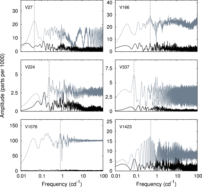
Figure 5: Amplitude spectrum of the archival (gray) and our new light curves (black). Mean noise levels are greatly reduced in new analysis.

4.1 Variability fractions

In this work, we found 823 new variables (V1484–V2306) and identified types of their variability. The discovery rate of new variables is increased by 60% in comparison with the existing catalog. The new variables are primarily 436 flaring stars, 30 sharp EBs, 48 low-amplitude pulsating variables, and 65 aperiodic variables, as well as many other rotating variables.

We briefly explored how variability fractions depends on their brightness/period and variable types. As shown in Figure 6, short-period, low-amplitude pulsating stars and episodic flare events are dominantly found at the bright- and faint-end of magnitude, respectively. In Figure 7, we plot variability fraction as a function of period. The period range of new variables is very similar to that reported by Hartman et al. (2008b). Of these, most of new pulsating candidates show $\delta$ Scuti-like characteristics ($P<$ 0.3 days). Also the majority of periodic variability can be explained by rotational modulation of surface features (i.e., starspots).

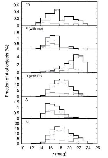
Figure 6: Variability fraction as a function of $r$ magnitude. Previously known variables (V1–V1483), newly detected variables (V1484–V2306), and total number of observed stars are marked with dashed lines, gray solid lines, and black solid lines, respectively.

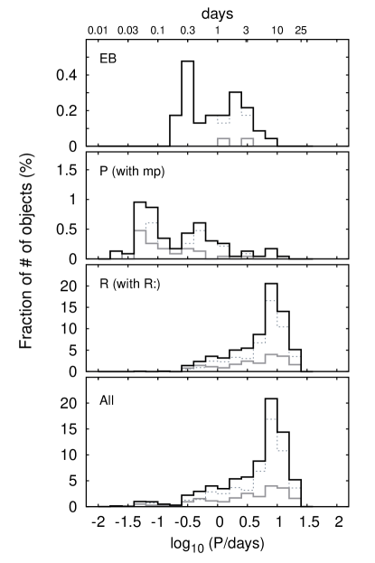
Figure 7: Variability fraction as a function of period. The representation of the lines is same as Figure 6.

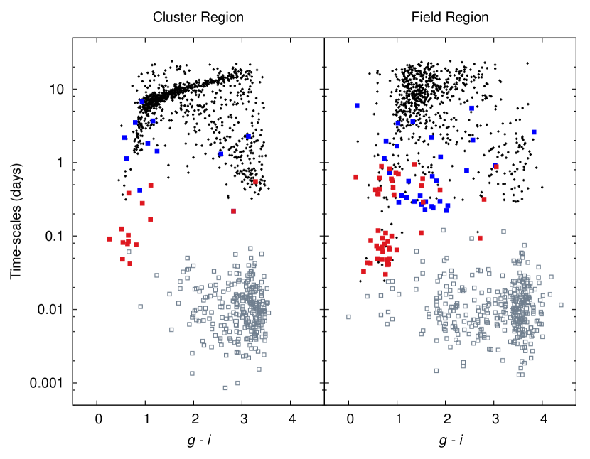
(a)

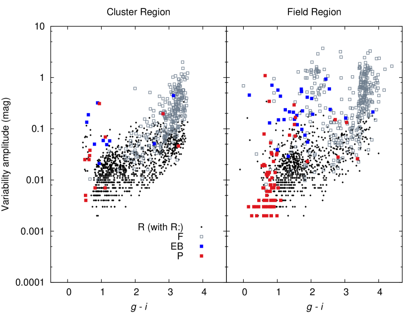
(b)

Figure 8: $g-i$ color vs. variability time-scales and amplitude relations for all periodic variables (black points) in the cluster and field region, respectively. For comparison purposes, we also show the parameter distributions of 625 flare events (gray squares). The flare time-scale is defined as the time duration of flare events at 80% of its peak level ($\tau_{0.2}$), and the flare amplitude is magnitude at the moment of flare maximum.

4.2 Time-scales and amplitudes of the variability

Time-scales and amplitudes of variability are intrinsic properties of the star and are independent of the distance (Eyer & Mowlavi, 2008). These two quantities can easily be measured from the light curves. We extracted the basic properties (e.g., period, amplitude) of all periodic variables using the Fourier decomposition technique. For comparison purposes, we utilized the flare parameters: (i) flare duration $\tau_{0.2}(=t_{0.2,rise}+t_{0.2,decay})$ that is defined as the time-scales of flare events at 80% of its peak level, and (ii) flare amplitude $\Delta$m_peak that is magnitude at the moment of flare maximum (S. -W. Chang et al., in preparation, hereafter Paper III).

We separate the variable objects into photometrically selected candidate cluster and field members provided by Hartman et al. (2008b), respectively. Since the $g-i$ color covers a relatively wide range from $-0.5$ to 4.5, we used $g-i$ as a separator between a sequence of cluster and that of field population. As can be seen in Figure 8, short period ($<$ 1 day), small amplitude pulsating stars are found at the blue-end of the distribution of both cluster and field sources, while episodic flare events are dominantly found from the sources in the red color range.

Our new data strengthen the relationship between the color of stars and their variability parameters derived for cluster members previously (Figure 8). The cluster members show a tight and nearly linear relation between color index and rotation period in the range of 1 $<$ $\log P$ $<$ 20 days, although the change in slope occurs after the knee point at $P$ $\simeq$ 7 days. This sequence forms a curved, diagonal band from bright blue stars to faint red ones, whose periods are increasing with increasing color index (or magnitude), while for non-cluster members there is no clear correlation.

The color-amplitude relation for the cluster members shows that, statistically, cooler stars have greater amplitudes in the case of both periodic variables and flares. As in the previous study on stellar rotation (see Section 6 and Figures 14, 15 and 17 in Hartman et al. 2009a), there is a strong correlation between Rossby number and amplitude, which can be interpreted as stars rotating faster having more spots, larger spots, and/or greater spot-photosphere contrast than slower rotating stars. Cooler stars have on average lower Rossby numbers at a particular age, so they end up having larger amplitudes.

4.3 Color-magnitude diagram of variable stars

Figure 9 illustrates the color-magnitude diagram (CMD) for all objects and all variable stars in the M37 field. In the new catalog, we found that about half of variable objects are distributed along the cluster main-sequence, and the other half are located in the field or in the outskirts of the cluster sequence. In order to identify the latter stars, we compared our data with the TRILEGAL model to reproduce the CMD at this location of the Galaxy. Most of the input parameters are described in the Girardi et al. (2005). For this analysis, we set the pointing parameters for the field center ($l=177.635$; $b=3.091$) and total field area ($\square$ = 0.16 deg²), a limiting magnitude as $r$ = 23.5 and a Salpeter initial mass function with cutoff at 0.01 M_☉. The remaining parameter values are fixed to default values that correspond to their model calibration. The model output consists mostly of thin disk stars (96%) with small contribution of old stars in the thick disk and halo (4%). Non-member, variable stars may be related in some way to the thin disk population, but their distributions are not fully explained by the model.

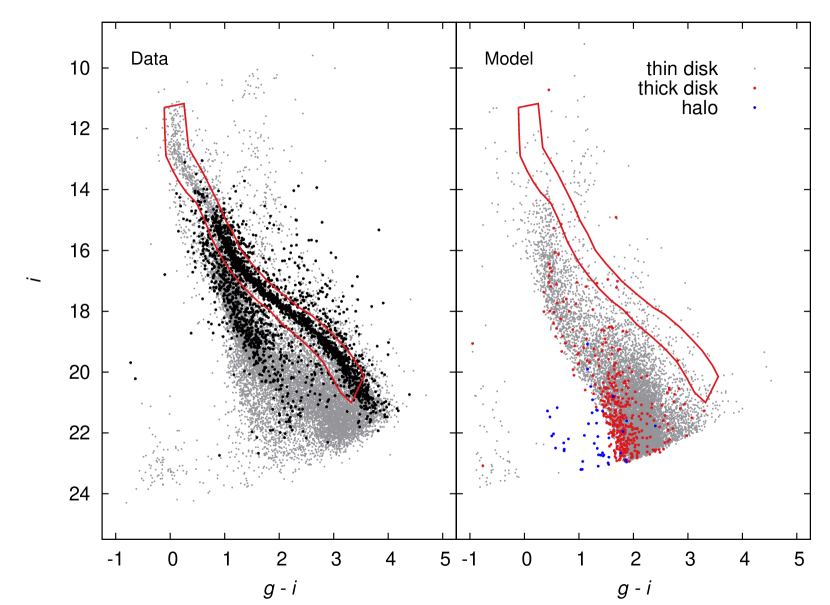
Figure 9: Color-magnitude diagram with marked positions of variables (black dots) found in the M37 field. We compare the $g-i$ vs. $i$ diagram of both observed (left) and simulated (right) data. Photometrically selected cluster region is plotted as red line in both panels.

5 Types of variability

In the following subsections, we investigate the nature of each variability class: (i) 61 EB systems, (ii) 92 multiperiodic variable stars, (iii) 132 aperiodic variables, and (iv) 436 flare stars, respectively. In order to understand variability properties, we utilized both color-magnitude and color-color diagrams to separate variable objects into broad magnitude ranges or spectral classes, to the extent possible.

5.1 Eclipsing binary star systems

Our photometric time-series data provide the light curves of 61 EBs. Figure 10 shows phased light curves of 8 newly discovered EBs. We categorize EBs into three groups according to the shape of phased light curves, and discuss each group below.

Figure 10: Phased light curves of 8 newly discovered eclipsing binaries.

5.1.1 Detached or Semi-detached EBs

EBs in this category are either Algol-type systems or $\beta$ Lyrae-type systems. To derive their geometric parameters, we used the Detached Eclipsing Binary Light curve (DEBiL) fitter by Devor (2005), which employs a simple model of a perfectly detached binary system in a classical 2-body orbit. Table 2 lists parameters derived for all detached/semi-detached binaries in the M37 field. EBs with well determined periods are included in DEBiL analysis. Special notes are given below for interesting features.

V2

This bright EB system was missed by previous study due to magnitude cut, but it clearly shows evidences of eclipse in our new light curve.

V587

The light curve of this EB system contains two distinct periodic signals, the 3.6173 days modulation with a small amplitude ($\Delta m$ $\simeq$ 0.056 mag) and an additional period at 3.2857 days (orbital period). Since an ellipsoidal variation should have the same period as the orbit, the first signal is more likely a consequence of starspots and rotational modulation.. After 3.6173-d modulation is removed, the light curve clearly shows the signature of a typical Algol-type binary with both primary and secondary eclipses.

V1482

This EB system is a newly recognized Algol-type binary with a $\delta$ Sct-type pulsating component. We have clearly detected an orbital period of 2.5972 days including multiple primary and secondary eclipses. The short period variability caused by stellar pulsation is shown in the out-of-eclipse light curves. In order to determine the oscillation modes of the pulsation, a frequency analysis was performed in the out-of-eclipse data using the program PERIOD04 (Lenz & Breger, 2005). Our analysis not only shows peaks as a consequence of binary effects ($f_{1}$ = 2.5638 and $f_{2}$ = 1.3006) but also reveals the presence of the dominant pulsation frequency $f_{3}$ = 0.0465 with a small amplitude ($\Delta m$ = 0.0035 mag).

Table 2: Parameters for 22 Detached and Semi-detached EB systems

		$r$	$P_{orb}$				$m_{1}$	$m_{2}$			$\omega$
No.	VarID	(mag)	(days)	$e$	$R_{1}/a$	$R_{2}/a$	(mag)	(mag)	sin($i$)	$t_{0}$	(deg)	Note
1	V1 (catalog V* V541 Aur)0	13.677	$\cdots$	$\cdots$	$\cdots$	$\cdots$	$\cdots$	$\cdots$	$\cdots$	$\cdots$	$\cdots$	Not enough data 0
2	V2 (catalog V* V540 Aur)0	14.840	$\cdots$	$\cdots$	$\cdots$	$\cdots$	$\cdots$	$\cdots$	$\cdots$	$\cdots$	$\cdots$	Not enough data 0
3	V55 (catalog Cl* NGC 2099 HGH V55)0	22.549	0.7780	$\leq$0.08	0.17	0.15	22.81	24.12	1.00	0.65	283.4	D0
4	V146 (catalog Cl* NGC 2099 HGH 330224)0	20.463	0.6477	$\cdots$	$\cdots$	$\cdots$	$\cdots$	$\cdots$	$\cdots$	$\cdots$	$\cdots$	SD; No secondary minimum? 0
5	V226 (catalog NGC 2099 HGH V226)0	22.121	0.9123	$\leq$0.01	0.10	0.04	22.23	24.59	1.00	0.53	129.5	D 0
6	V395 (catalog NGC 2099 HGH V395)0	17.392	3.4460	0.01	0.10	0.08	17.96	18.35	1.00	0.33	232.1	D0
7	V457 (catalog NGC 2099 HGH V457)0	19.474	2.1995	$\leq$0.08	0.08	0.07	20.15	20.30	1.00	0.75	239.7	D0
8	V485 (catalog 2MASS J05520131+3232509)0	17.080	1.6676	$\cdots$	$\cdots$	$\cdots$	$\cdots$	$\cdots$	$\cdots$	$\cdots$	$\cdots$	D; No secondary minimum? 0
9	V587 (catalog Cl* NGC 2099 HGH V587)0	16.572	3.2857	0.52	0.06	0.02	16.58	21.24	1.00	0.31	209.4	D + RM (P=3.6173 days) (new)0
10	V692 (catalog Cl* NGC 2099 HGH V692)0	16.669	1.8324	0.06	0.28	0.06	16.73	19.80	0.98	0.01	77.2	SD 0
11	V716 (catalog Cl* NGC 2099 HGH V716)0	21.635	2.0272	$\cdots$	$\cdots$	$\cdots$	$\cdots$	$\cdots$	$\cdots$	$\cdots$	$\cdots$	D; No secondary minimum?0
12	V733 (catalog Cl* NGC 2099 HGH V733)0	17.383	0.7310	$\leq$0.04	0.43	0.34	17.61	18.91	0.99	0.77	73.3	D 0
13	V965 (catalog Cl* NGC 2099 HGH V965)0	16.736	1.9732	0.00	0.16	0.05	16.75	21.05	1.00	0.27	357.0	SD (new) 0
14	V1028 (catalog 2MASS J05523843+3223296)0	18.730	5.4956	0.03	0.04	0.04	19.21	19.84	1.00	0.55	267.5	D + RM0
15	V1141 (catalog 2MASS J05524614+3239336)0	16.977	3.6948	$\leq$0.66	0.06	0.01	16.98	22.60	1.00	0.29	268.3	D0
16	V1182 (catalog Cl* NGC 2099 HGH V1182)0	21.869	2.2834	0.05	0.07	0.06	22.40	22.87	1.00	0.16	268.3	D (new)0
17	V1187 (catalog Cl* NGC 2099 HGH V1187)0	19.742	1.1919	$\leq$0.41	0.12	0.02	19.77	23.56	1.00	0.86	271.6	D0
18	V1380 (catalog 2MASS J05531108+3224434)0	14.874	2.1898	$\leq$0.05	0.16	0.06	15.01	17.19	0.99	0.84	280.1	D + $\gamma$ Doradus component (P=0.941/1.174 days)0
19	V1456 (catalog Cl* NGC 2099 HGH S2)0	17.006	5.9680	0.12	0.07	0.07	17.47	18.15	1.00	0.54	89.3	D0
20	V14820	15.597	2.5972	0.02	0.14	0.08	15.71	18.14	0.99	0.17	76.1	D + $\delta$ Scuti component (P=0.0465 days) (new)0
21	V21380	14.181	3.4051	0.04	0.09	0.04	14.28	16.85	1.00	0.63	191.7	D (new)0
22	V22970	15.863	3.5109	$\leq$0.01	0.12	0.02	15.88	20.42	1.00	0.32	229.7	D (new)0

Note. — The column description is as follows. $e$: Orbital eccentricity; $R_{1}/a$: Radius of large star (in units of semimajor axis); $R_{2}/a$: Radius of small star (in units of semimajor axis); $m_{1}$: Brightness of large star (magnitudes); $m_{2}$: Brightness of small star (magnitudes); sin($i$): Sine of inclination; $t_{0}$: Phased epoch of periastron; $\omega$: Argument of periastron (in degrees).

5.1.2 Contact EBs

The light curves of contact binary stars (also known as W UMa-type variable stars; EW) are very much different from those for detached binaries. Our new catalog lists 22 contact binaries of which four are new discoveries (V840, V1031, V1250, V1463).

V37, V706, V1031

These systems are one of the fastest orbiting contact binary systems ($P$ $\simeq$ 0.22 days). It is known that observed distribution of orbital periods has a cut-off period limit at 0.22 days (e.g., Rucinski 1992, 2002; Molnar et al. 2013). We have not found anything faster in our study.

(a)

(b)

Figure 11: Zoomed-in light curve collection of eclipse candidates. Short vertical lines in the middle of each panel mark epochs of eclipses. The numbers in the upper right denote the duration ($\Delta t$) between the start time of eclipse and the end.

Table 3: List of new 15 eclipsing binary candidates from CPA analysis

		Star	$r$	$N_{\mathrm{event}}$	$t_{\mathrm{0}}$	$\Delta t$	$d$
No.	VarID	(J2000)	(mag)	(#)	(day)	(hour)	(mag)
1	V791 (catalog 2MASS J05522390+3228262)0	055223.89+322826.470	15.604	10	53732.28145	1.0	0.011
				20	53734.26454	2.6	0.142
				30	53756.09692	3.1	0.134
2	V827 (catalog 2MASS J05522624+3240446)0	055226.24+324044.620	15.774	10	53731.14064	1.1	0.074
				20	53745.26403	4.7	0.171
3	V926 (catalog Cl* NGC 2099 HGH V926)0	055232.65+322208.160	16.348	10	53755.08741	2.2	0.046
4	V985 (catalog Cl* NGC 2099 HGH V985)0	055236.13+323001.130	16.012	10	53734.15888	2.2	0.054
				20	53756.24427	1.1	0.051
5	V1018 (catalog Cl* NGC 2099 HGH V1018)0	055237.96+323415.640	16.569	10	53732.14053	1.5	0.019
				20	53756.17928	1.8	$<$ 0.030
6	V1483 (catalog Cl* NGC 2099 HGH S29)0	055311.98+322353.580	17.717	10	53726.20141	0.4	0.208
				20	53730.29695	0.7	0.146
				30	53733.22359	1.6	0.184
				40	53734.41413	0.4	0.159
				50	53737.34213	1.2	0.161
				60	53740.33536	0.9	0.124
				70	53753.25941	0.7	0.203
				80	53756.17828	1.2	0.157
7	V17310	055157.49+324534.900	15.823	10	53728.25931	3.3	0.233
				20	53732.11914	2.5	0.282
8	V17480	055159.96+322433.640	14.846	10	53740.46821	0.5	0.012
				20	53742.46911	0.5	0.015
9	V17570	055201.06+322408.790	17.189	10	53731.14064	0.4	0.022
10	V18890	055216.11+322822.950	14.971	10	53742.42521	1.6	0.100
				20	53756.13038	3.8	0.082
11	V18920	055216.39+322609.000	19.328	10	53734.15888	2.0	0.178
12	V19090	055218.62+324100.160	13.281	10	53731.34461	0.0	0.019
				20	53753.15826	2.0	0.291
13	V19150	055218.84+324434.080	21.189	10	53755.21194	1.9	0.273
14	V22130	055301.96+323744.910	16.433	10	53725.17392	2.0	0.230
				20	53733.15900	0.5	0.025
15	V2214 (catalog Cl* NGC 2099 HGH 80009)0	055302.02+322327.620	15.094	10	53732.11914	2.6	0.091
				20	53735.16000	1.9	0.087
				30	53754.14737	0.8	0.051

5.1.3 New EB candidates with eclipsing-like features

With our CPA analysis, we discovered 15 new eclipsing binary candidates that have eclipsing-like or transit-like features undergoing eclipse, eclipse-ingress, or eclipse-egress phases. Table 3 summarize observed eclipsing features of the light curves, which are missed by the standard analysis software. Their orbital periods are not well constrained. The light curve of each event can be described by the first time of dimming points $t_{\mathrm{0}}$, the time duration between the start time of eclipse and the end time of eclipse $\Delta t$, and the depth of observed dimming points $d$. Figure 11 illustrates examples of light curves of this category.

V791

This detached EB system has deep primary and secondary eclipses (12–13% and 1%, respectively), and has out-of-eclipse variability at the 2% level with period $\sim$4.0631 days. After pre-whitening with the rotational modulation, our analysis indicates possible orbital period $P_{\mathrm{orb}}$ = 2.4277 days.

V926

This object was known to be a long-period (16.5777 days) variable star. Our LS analysis supports the conclusion of previous study, but it has sinusoidal-shaped periodic signal in our light curve. The LS periodogram shows two power peaks with periods similar to previous one (rank 1 = 15.7291 days) and another shorter than one day (rank 2 = 0.9376 days). One sudden eclipse event was caught during its return to quiescence brightness.

Figure 12: Phased light curves of V985, V1483, V1731, and V1889. The mid-eclipse is set to the orbital phase of 0.5. The estimated orbital period is given in the upper right of each panel.

V1018

We caught two eclipses, but the star seems to vary all the time in a strange manner.

5.1.4 Grazing EB candidates

By using the Plavchan algorithm (Plavchan et al., 2008) provided in NASA Exoplanet Archive Periodogram Service, we identified two types of systems which can be confused with a transiting planetary system. One type is connected with the grazing EBs, and it shows V- or U-shape eclipses. The other type is the eclipsing binary systems with a large primary star, in which case the eclipse produces a flat bottomed light curve with small deeming. Figure 12 shows the phased light curves of actual cases of these contaminants. The observed shapes of the eclipsing events resemble transit-like signals, but depths of mid-eclipse are more than a few % of the total light (V985: 5%; V1483: 14%; V1731: 24%; V1889: 10%).

5.2 Multiperiodic variable stars

Multi-periodicity is a common feature found in nearly all type of pulsating stars such as $\delta$ Scuti stars, RR Lyraes, and Cepheids. Our catalog contains many examples of multiperiodic variable stars which deserve in-depth analysis.

We performed multiple-frequency analysis of 92 short-periodic variables with the program PERIOD04 (Lenz & Breger, 2005), looking for the presence of multi-periodicity. With an iterative pre-whitening procedure, discrete Fourier transformations are calculated until there is no meaningful change in the fit residuals. Each light curve was fitted using an equation of the form:

$$y(t)=A_{0}+\sum_{j=1}^{n}A_{j}\cos(2\pi f_{j}t-\phi_{j})$$ (9)

where $A_{0}$ is a mean level and $f_{j}$, $A_{j}$, and $\phi_{j}$ are the frequency, amplitude, and phase for each successive peak found in the amplitude spectrum. We adopt a conservative approach in selecting the statistical significant peaks from the amplitude spectrum. In general, a signal/noise (S/N) amplitude ratio of 4.0 is a good criterion for independent frequencies, equivalent to 99.9% certainty of variability (Breger et al., 1993; Kuschnig et al., 1997). For combination modes with known values, the S/N amplitude ratio of $\sim$3.5 is used which is equivalent to 90% certainty. After removal of all significant peaks in the amplitude spectrum, the noise level was estimated on the residual amplitude spectrum over 5 c/d boxes around each frequency. The resulting light curve of one example multiperiodic variable is shown in Figure 13. The multi-period model is in excellent agreement with the observed light curve.

Figure 13: Example light curve of multiperiodic variable V1898. The fit of the 16-frequency solution presented in the Table A2 is shown as a solid curve. The full amplitude of this variation is about 0.04 mag in $r$-band light curve.

Table A2 summarizes all candidate frequencies identified in 92 multiperiodic light curves with their fitted Fourier parameters. All the detected frequencies are classified as independent modes ($f_{1}$, $f_{2}$, $f_{3}$, $\cdots$), combination modes ($af_{i}\pm bf_{j}$), and harmonic mode ($hf_{j}$).

5.3 Aperiodic variability

By using the method described in Section 3.1, we detected long-term aperiodic variability of 132 variable candidates with time-scales similar to the total observing time span ($\sim$31 days). We visually inspected each light curve to confirm its variable nature, and this result is illustrated in terms of time sequence (Figure 14). Due to the lack of periodicity, the light curves of aperiodic variables are simply characterized by the level of photometric variability ($\Delta m$), the dispersion about the mean level ($\sigma_{m}$), and the reduced chi-square assuming a constant median value for the light curve ($\chi_{\nu}^{2}$).

$$\chi_{\nu}^{2}=\frac{1}{N-1}\sum_{i}^{N}\frac{(x_{i}-\bar{x})^{2}}{\sigma_{i}^{2}}$$ (10)

where $\sigma_{i}$ is the photometric uncertainty of each data point $x_{i}$, and $N$ is the total number of measurements. The full parameters are described in Table A3. These variables show relatively low levels of variability with $\Delta m$ $<$ 0.03 mag (60%) and $\Delta m$ $<$ 0.05 mag (80%), respectively.

Figure 14: Examples of aperiodic light curves showing variations about the mean, in addition to a relatively long-term variability on timescales similar to the total observing time span ($\sim$31 days).

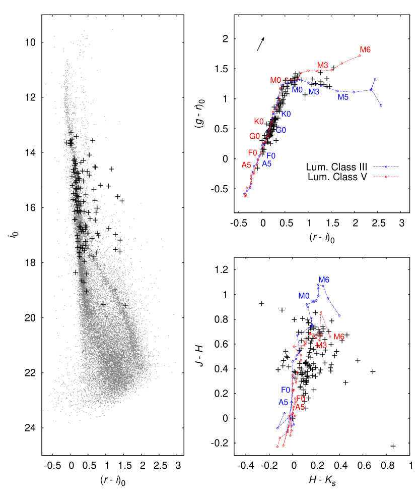
Figure 15: Color-magnitude diagram and color-color diagrams of aperiodic variable candidates (black points). The color index distributions follow the locus of normal stars taken from Covey et al. (2007). The two lines show the location of the median stellar locus of dwarf (V) and giant (III) stars having solar-metallicity. The cluster’s extinction is taken into account for SDSS color-color diagram. In order to derive $A_{\lambda}/A_{V}$ values for SDSS photometry system, we used the extinction coefficients compiled in Girardi et al. (2004).

We used the combined SDSS and 2MASS photometry to identify basic properties of these sources. Since color ranges are much smaller in the near-infrared color-color diagram, the stellar locus is not as well defined as in optical color-color diagram (Figure 15). We infer spectral types from Covey et al. (2007), in which stars in this sample cover spectral types from approximately A5 to M5 and can be either main-sequence and giant stars. The CMD indicates that many of these aperiodic stars are field stars not associated with M37.

The origin of aperiodic nature is difficult to explain. Possible speculations include that (i) some of these may be cases where long-period field giants are detected as low-amplitude photometric variables on timescales of weeks or longer (e.g., Henry et al. 2000; Ciardi et al. 2011), (ii) some of them may be semi-regular variables exhibiting both fast and slow variabilities (e.g., Andronov & Chinarova 2013), and (iii) as mentioned in Hartman et al. (2008b), the rapid amplitude variation may be flickering, nova-like outbursts seen in many symbiotic variables (e.g., Gromadzki et al. 2009, 2013). Further observations of much longer duration will be necessary to properly characterize these aperiodic variables.

5.4 Flare stars

Earlier analysis of M37 data (Hartman et al. 2008a) could not address flare events properly because many data points were removed as outliers. Our new pipeline, with nearly 100% data utilization, offers opportunity to investigate flare stars more thoroughly.

By CPA analysis, we found that 436 stars (625 flare events) show flaring activity characterized by a rapid flux increase and a slower decay. As expected, the location of these flaring stars on color-magnitude and color-color diagrams suggest that most of them are late-type main-sequence stars (K4–M6) in M37 open cluster (Figure 16). Flares are also observed from earlier spectral types (A0–K3), but these are only a few and probably belong to field stars.

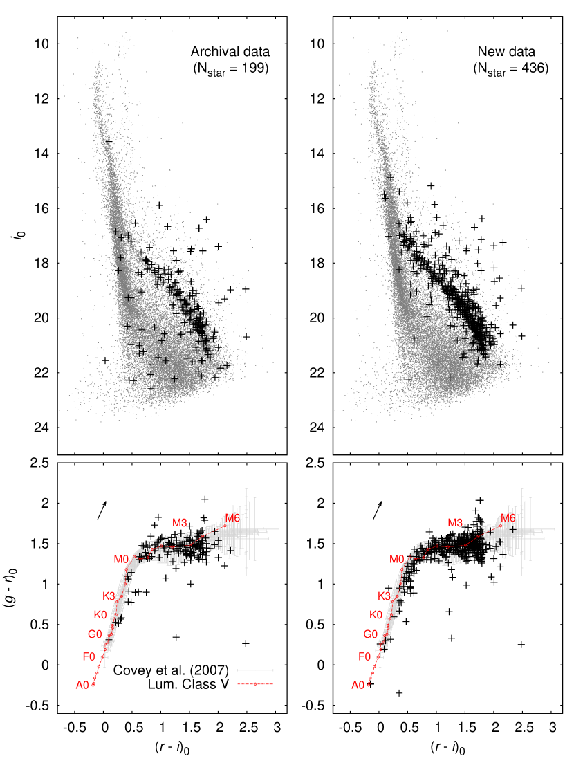
Figure 16: Color-magnitude and color-color diagrams of flaring stars, detected in archival (left panels) and our new data (right panels), respectively. The red lines represent the main-sequence stellar locus with solar metallicity (Covey et al., 2007). Most of these stars can be regarded as late-type main sequence stars (K4–M6) in the M37 open cluster.

The underlying mechanism of flares in stars cooler than about F5 is essentially the same as in the Sun. It is believed that these cool stars can generate a magnetic field through a dynamos at the interface between the radiative core and the convective envelope (Benz & Güdel, 2010). Thus, flaring is an inevitable result of strong magnetic field. But flares in hot stars, especially in A-type stars, are not easy to explain in the context of dynamo process because these stars should not generate strong magnetic fields in their thin convection layer and are incapable of storing larger energy in that region (Balona, 2012).

The observed flare signature of one A-type star (V72) might be the result of binarity. If an A-type main sequence star has an active M dwarf secondary star, such binary star would look like a flare-generating A-type star.

The number of flare events is increased by a factor of two in the new analysis because our new calibration procedure provides more accurate $r$-band light curves (Figure 17). In Table A4 and Figure 18, we list the parameters of flare events discovered by our CPA analysis. They have a broad range of peak amplitude ($\Delta m_{\mathrm{peak}}$ = $0.006\sim 3.719$ mag) and typical durations of a few minutes to several hours, irrespective of their spectral type. More detailed analysis of flare statistics and its relation to magnetic activity and stellar rotation will be presented in subsequent papers.

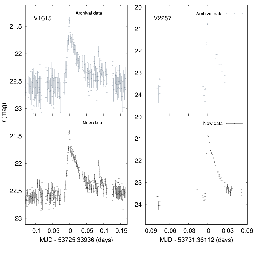
Figure 17: Comparison between our and archival light curves of the two flare events. As shown in Paper I, new analysis provides more improved $r$-band data in terms of both photometric accuracy and data recovery rate.

(a)

(b)

(c)

Figure 18: Various light curves of discovered flare events selected by color cut ($(g-r)_{0}<1$). Most of them show a sharp rise and subsequent exponential decay.

6 Conclusion

We cataloged and investigated a variety of photometric variables in the field of M37 using our new light curves, which were obtained from archival imaging data of one-month long exo-planet transit survey with the 6.5-m MMT telescope. This new dataset allows a rare opportunity to explore different types of variability of short ($\sim$minutes) and long ($\sim$one-month) time-scales simultaneously.

We find 61 eclipsing binary systems (EB), 92 multiperiodic variable stars (mp), 132 aperiodic variables (A), and 436 flare stars (F), as well as several hundreds of rotating variables (R). Our work has increased the number of known variable stars in this field by 60%. The new variable catalog has been made available on the web (http://stardb.yonsei.ac.kr/).

Table A1: New catalog of 2306 variable stars in M37 field

	StarID	Period	Amp	$u$	$r$	$g-r$	$r-i$	$z$	$V$	$B-V$	$J$	$J-H$	$H-K_{s}$
VarID	(J2000)	(days)	(mag)	(mag)	(mag)	(mag)	(mag)	(mag)	(mag)	(mag)	(mag)	(mag)	(mag)	VarType
V1 (catalog V* V541 Aur)0	055220.39+323319.650	$\cdots$	$\cdots$	$\cdots$	13.677	0.285	0.191	$\cdots$	13.406	0.609	12.447	0.270	0.063	EB0
V2 (catalog V* V540 Aur)0	055216.58+322815.320	$\cdots$	$\cdots$	16.792	14.840	0.564	0.290	14.471	14.653	0.688	13.539	0.287	0.134	EB0
V3 (catalog V* V542 Aur)0	055233.01+323241.910	0.4225	0.320	17.982	15.789	0.560	0.329	15.284	16.051	0.728	14.267	0.355	0.012	EB0
V4 (catalog V* V544 Aur)0	055253.26+323301.470	0.5582	0.235	18.079	15.634	0.762	0.477	15.093	15.948	0.938	13.951	0.497	0.101	EB0
V5 (catalog V* V545 Aur)0	055300.63+322450.810	0.2788	0.310	18.036	15.915	0.459	0.481	15.235	16.184	0.585	14.421	0.359	0.084	mp0
V6 (catalog V* V539 Aur)0	055150.53+323234.700	0.1098	0.343	18.218	15.973	0.591	0.173	15.622	$\cdots$	$\cdots$	14.739	0.342	-0.009	mp0
V7 (catalog Cl* NGC 2099 HGH V7)0	055239.09+323631.270	0.3577	0.433	19.858	17.252	1.039	0.056	17.065	17.890	0.815	15.779	0.446	0.196	EB0
V8 (catalog Cl* NGC 2099 KV 1)0	055234.32+323218.700	0.1195	$\cdots$	$\cdots$	$\cdots$	$\cdots$	$\cdots$	$\cdots$	$\cdots$	$\cdots$	$\cdots$	$\cdots$	$\cdots$	U0
V9 (catalog 2MASS J05521491+3224415)0	055214.91+322441.350	0.0909	$\cdots$	14.873	13.233	0.137	0.128	13.114	13.298	0.370	12.348	0.171	0.042	P0
V10 (catalog 2MASS J05520049+3236481)0	055200.49+323648.190	0.9432	0.075	16.844	14.151	0.928	0.436	13.493	14.762	0.531	12.356	0.567	0.131	P0

Note. — Table A1 is published in its entirety in the electronic edition of Astronomical Journal. A portion is shown here for guidance regarding its form and content.

Table A2: Candidate frequencies identified in 92 multiperiodic light curves

		Star	$r$	Frequency	Frequency	$A_{r}$	$\phi$
No.	VarID	(J2000)	(mag)	(cd-1)	name	(mmag)	(deg)	S/N	Note
1	V5 (catalog V* V545 Aur)0	055616.79+322514.200	15.915	3.5872	f10	310.1	0.3331	68.9
				7.1768	f2(=2f1)0	35.4	0.2906	11.3
				10.7619	f3(=3f1)0	22.8	0.0418	10.3
				5.6768	f40	19.5	0.2369	5.7
				14.3473	f50	13.8	0.9990	7.1
2	V6 (catalog V* V539 Aur)0	055506.89+323303.200	15.973	9.1040	f1(=f3-f2)0	343.4	0.5433	172.7
				18.2081	f2(=f3-f1)0	89.9	0.2201	53.6
				27.3122	f3(=f1+f2)0	27.6	0.9237	19.7
				8.7545	f40	15.4	0.5801	8.1
				11.9319	f50	14.5	0.5557	6.3
				36.4178	f6(=2f2)0	10.1	0.0527	10.4
				14.9868	f70	8.8	0.9887	4.5
				16.8695	f80	7.9	0.7280	4.5
3	V11 (catalog 2MASS J05520338+3235136)0	055519.81+323541.230	15.245	8.4261	f10	79.0	0.9052	84.8
				16.8561	f2(=2f1)0	7.6	0.6488	8.3
				17.7044	f30	8.0	0.5895	9.1
				16.4751	f40	6.9	0.5617	7.3
				8.8787	f50	4.9	0.4440	5.2
				12.0801	f60	4.8	0.8357	5.0
				9.2640	f70	5.9	0.6453	6.4
				10.6455	f80	5.4	0.0597	6.0
				13.5604	f90	4.8	0.8005	4.9
				16.2578	f100	5.1	0.6379	5.3
				8.0470	f110	4.5	0.8268	4.7
				2.3825	f120	5.2	0.7274	3.6
				4.3812	f130	4.3	0.3942	4.2
				14.9483	f140	3.9	0.8404	4.0
4	V12 (catalog 2MASS J05524469+3230167)0	055600.99+323041.250	15.873	12.7176	f10	14.4	0.0994	8.1
				7.8896	f20	13.8	0.4901	6.0
				12.7698	f30	10.5	0.0175	6.0	close to f10
				14.4564	f40	9.6	0.0884	6.5
5	V13 (catalog 2MASS J05521116+3225159)0	055527.32+322543.010	16.511	10.0341	f1(=f12-f2)0	23.0	0.4259	137.9
				10.4706	f2(=f12-f1)0	13.0	0.8171	77.9
				17.1389	f30	8.7	0.9050	51.9
				14.0376	f40	6.1	0.6801	33.6
				13.0968	f50	3.7	0.1837	20.9
				12.8019	f60	3.1	0.2056	17.4
				15.0841	f70	2.1	0.7887	11.6
				13.6263	f80	1.3	0.1260	7.1
				11.1091	f90	1.4	0.2454	8.7
				27.1718	f100	1.0	0.7296	6.7

Note. — Table A2 is published in its entirety in the electronic edition of Astronomical Journal. A portion is shown here for guidance regarding its form and content.

Table A3: Long-term 132 aperiodic variable candidates with timescales of $>$1 month

		Star	$r$	$\sigma_{m}$	$\Delta$$m$
No.	VarID	(J2000)	(mag)	(mag)	(mag)	$\chi^{2}_{\nu}$	NLC	Note
1	V58 (catalog Cl* NGC 2099 HGH V58)0	055122.14+322942.400	16.742	0.009	0.096	443.5	4730	$\cdots$
2	V70 (catalog Cl* NGC 2099 HGH V70)0	055123.93+324357.220	15.837	0.003	0.017	14.0	4706	$\cdots$
3	V75 (catalog Cl* NGC 2099 HGH V75)0	055124.73+324312.360	18.360	0.004	0.028	1.8	4730	13.260
4	V87 (catalog Cl* NGC 2099 HGH V87)0	055125.42+323600.450	17.564	0.002	0.017	1.6	4730	21.199
5	V107 (catalog Cl* NGC 2099 HGH V107)0	055127.04+323225.570	15.458	0.002	0.010	7.7	4592	$\cdots$
6	V114 (catalog Cl* NGC 2099 HGH V114)0	055128.19+322931.140	17.854	0.004	0.029	3.4	4730	$\cdots$
7	V131 (catalog Cl* NGC 2099 HGH V131)0	055129.26+323235.440	18.515	0.005	0.029	1.4	4730	$\cdots$
8	V147 (catalog Cl* NGC 2099 HGH V147)0	055130.48+324053.050	18.348	0.005	0.033	1.9	4730	7.709
9	V157 (catalog Cl* NGC 2099 HGH V157)0	055131.24+323059.610	17.688	0.008	0.046	12.9	4730	$\cdots$
10	V163 (catalog Cl* NGC 2099 HGH V163)0	055131.87+324233.830	17.482	0.004	0.026	5.1	4730	$\cdots$

Note. — Table A3 is published in its entirety in the electronic edition of Astronomical Journal. A portion is shown here for guidance regarding its form and content.

Table A4: 436 flare stars

		Star	$r$	Flareevent	$t_{\mathrm{peak}}$	$\Delta$mpeak	$\tau_{0.2}$
No.	VarID	(J2000)	(mag)	(No.)	(days)	(mag)	(hours)	Note
1	V42 (catalog Cl* NGC 2099 HGH V42)0	055120.47+322200.750	20.690	10	53742.40307	0.093	0.17
				20	53742.46247	0.135	0.08
2	V50 (catalog Cl* NGC 2099 HGH V50)0	055121.46+322856.900	19.990	10	53730.34740	0.221	0.55
				20	53733.19093	0.176	0.21
				30	53735.19767	0.039	0.49
				40	53737.33376	0.188	0.30
3	V69 (catalog Cl* NGC 2099 HGH V69)0	055123.45+322948.830	20.809	10	53732.22482	0.061	0.32
				20	53732.35513	0.133	1.11
				30	53742.35427	0.281	0.23
4	V72 (catalog Cl* NGC 2099 HGH V72)0	055124.44+324407.710	15.143	10	53730.32306	0.010	1.47
5	V76 (catalog Cl* NGC 2099 HGH V76)0	055124.78+323440.560	18.368	10	53728.24480	0.026	0.17
				20	53742.44376	0.117	0.24
				30	53753.25302	0.139	0.16
6	V78 (catalog Cl* NGC 2099 HGH V78)0	055124.82+322937.320	20.017	10	53726.39533	0.046	0.10	Var0
7	V86 (catalog Cl* NGC 2099 HGH V86)0	055125.41+323800.030	18.086	10	53726.27563	0.041	0.58	Var0
				20	53727.30272	0.025	0.46
8	V91 (catalog Cl* NGC 2099 HGH V91)0	055125.71+323106.380	20.553	10	53734.23990	0.072	0.20	Var0
				20	53756.08268	0.079	0.60
9	V104 (catalog Cl* NGC 2099 HGH V104)0	055126.78+324024.730	17.971	10	53726.43908	0.030	0.29
10	V112 (catalog Cl* NGC 2099 HGH V112)0	055127.86+322854.790	22.181	10	53727.19210	0.360	0.58	Var0

Note. — Table A4 is published in its entirety in the electronic edition of Astronomical Journal. A portion is shown here for guidance regarding its form and content.

References

- Abazajian et al. (2009) Abazajian, K. N., Adelman-McCarthy, J. K., Agűeros, M. A., et al. 2009, ApJS, 182, 543
- Andronov & Chinarova (2013) Andronov, I. L. & Chinarova, L. L. 2013, arXiv:1308.1129
- Balona (2012) Balona, L. A. 2012, MNRAS, 423, 3420
- Benkő et al. (2010) Benkő, J. M., Kolenberg, K., Szabó, R., et al. 2010, MNRAS, 409, 1585
- Benz & Güdel (2010) Benzm, A. O. & Güdel, M. 2010, ARA&A, 48, 241
- Breger et al. (1993) Breger, M., Stich, J., Garrido, R., et al. 1993, A&A, 271, 482
- Butler & Bloom (2011) Butler, N. R. & Bloom, J. S. 2011, AJ, 141, 93
- Chang et al. (2015) Chang, S.-W., Byun, Y.-I., & Hartman, J. D. 2015, AJ, 149, 135 (Paper I)
- Ciardi et al. (2011) Ciardi, D. R., Braun, K. V., Bryden, G., et al. 2011, AJ, 141, 108
- Covey et al. (2007) Covey, K. R., Ivezić, Ž., Schlegel, D., et al. 2007, AJ, 134, 2398
- Cutri et al. (2003) Cutri, R. M., Skrutskie, M. F., van Dyk, S., et al. 2003, The IRSA 2MASS All-Sky Point Source Catalog, NASA/IPAC Infrared Science Archive, http://irsa.ipac.caltech.edu/applications/Gator/
- Debosscher et al. (2007) Debosscher, J., Sarro, L. M., Aert, C., et al. 2007, A&A, 475, 1159
- Debosscher et al. (2009) Debosscher, J., Sarro, L. M., López, M., et al. 2009, A&A, 506, 519
- Devor (2005) Devor, J. 2005, ApJ, 628, 411
- Eyer & Mowlavi (2008) Eyer, L. & Mowlavi, N. 2008, J. Phys. Conf. Ser., 118, 012010
- Girardi et al. (2004) Girardi, L., Grebel, E. K., Odenkirchen, M., & Chiosi, C. 2004, A&A, 422, 205
- Girardi et al. (2005) Girardi, L., Groenewegen, M. A. T., Hatziminaoglou, E., & da Costa, L. 2005, A&A, 436, 895
- Glicenstein (2001) Glicenstein, J. -F. 2001, in ASP Conf. Ser. 239, Microlensing 2000: A New Era of Microlensing Astrophysics, ed. J. W. Menzies & Penny D. Sackett. (San Francisco, CA:ASP), 28
- Gromadzki et al. (2009) Gromadzki, M., Mikołajewska, J., Whitelock, P., & Marang, F. 2009, Acta Astron., 59, 169
- Gromadzki et al. (2013) Gromadzki, M., Mikolajewska, J., & Soszynski, I. 2013, arXiv:1312.6063
- Gruberbauer et al. (2007) Grubrbauer, M., Kolenberg, K., Rowe, J. F., et al. 2007, MNRAS, 379, 1498
- Guggenberger et al. (2012) Guggenberger, E., Kolenberg, K., Nemec, J. M., et al. 2012, MNRAS, 424, 649
- Hartman et al. (2008a) Hartman, J. D., Gaudi, B. S., Holman, M. J., et al. 2008a, ApJ, 675, 1233
- Hartman et al. (2008b) Hartman, J. D., Gaudi, B. S., Holman, M. J., et al. 2008b, ApJ, 675, 1254
- Hartman et al. (2009a) Hartman, J. D., Gaudi, B. S., Pinsonneault, M. H., et al. 2009a, ApJ, 691, 342
- Hartman et al. (2009b) Hartman, J. D., Gaudi, B. S., Holman, M. J., et al. 2009b, ApJ, 695, 336
- Henry et al. (2000) Henry, Gregory W., Fekel, Francis C., Henry, Stephen M., & Hall, Douglas S. 2000, ApJS, 130, 201
- Irwin et al. (2007) Irwin, J., Irwin, M., Aigrain, S., et al., MNRAS, 375, 1449
- Kalirai et al. (2001) Kalirai, J. S., Ventura, P., Richer, H. B., et al. 2001, AJ, 122, 3239
- Kang et al. (2007) Kang, Y. B., Kim, S.-L., Rey, S.-C., et al. 2007, PASP, 119, 239
- Kelly et al. (2009) Kelly, B. C., Bechtold, J., & Siemiginowska, A. 2009, ApJ, 698, 895
- Kiss et al. (2001) Kiss, L. L., Szabó, Gy. M., Sziládi, K., Fürész, G., Sárneczky, K., & Csák, B. 2001, A&A, 376, 561
- Kovács et al. (2002) Kovács, G., Zucker, S., & Mazeh, T. 2002, A&A, 391, 369
- Kuschnig et al. (1997) Kuschnig, R., Weiss, W. W., Gruber, R., Bely, P. Y., Jenkner, H. 1997, A&A, 328, 544
- Lenz & Breger (2005) Lenz P., Breger M. 2005, CoAst, 146, 53
- Lomb (1976) Lomb, N. R. 1976, Ap&SS, 39, 447
- Messina et al. (2008) Messina, S., Distefano, E., Parihar, P., et al. 2008, A&A, 483, 253
- Molnar et al. (2013) Molnar, Lawrence A., Van Noord, Daniel M., & Steenwyk, Steven D. 2013, arXiv:1310.0539
- Richards et al. (2011) Richards, J. W., Starr, D. L., Butler, N. R., et al. 2011, ApJ, 733, 10
- Rucinski (1992) Rucinski, S. M. 1992, AJ, 103, 960
- Rucinski (2002) Rucinski, S. M. 2002, PASP, 114, 1124
- Palmer (2009) Palmer, D. M. 2009, ApJ, 695, 496
- Plavchan et al. (2008) Plavchan, P., Jura, M., Kirkpatrick, D., Cutri, Roc M., & Gallagher, S. C. 2008, ApJS, 175, 191
- Press & Rybicki (1989) Press, W.H. & Rybicki, G.B. 1989, ApJ, 338, 277
- Press et al. (1992) Press, W. H., Teukolsky, S. A., Vetterling, W. T., & Flannery, B. P. 1992, Numerical Recipes in C. 2nd ed. (New York: Cambridge University Press)
- Reegen (2007) Reegen, P. 2007, A&A, 467, 1353
- Samus et al. (2009) Samus, N. N., Durlevich, O. V., Kazarovets, E. V., et al. 2009, VizieR Online Data Catalog:B/gcvs, 1, 2025
- Scargle (1982) Scargle, J. D. 1982, ApJ, 263, 835
- Schütz & Holschneider (2011) Schütz, N. & Holschneider, M. 2011, Phys. Rev. E, 84, 021120
- Schwarzenberg-Czerny (1989) Schwarzenberg-Czerny, A. 1989, MNRAS, 241, 153
- Shin & Byun (2004) Shin, M.-S. & Byun, Y.-I. 2004, JKAS, 37, 79
- Taylor (2000) Taylor, W. 2000, in Change-Point Analyzer 2.0 shareware program, Taylor Enterprises, Libertyville, Illinois., http://www.variation.com/cpa