Comparing Large Covariance Matrices under Weak Conditions on the Dependence Structure and its Application to Gene Clustering

Abstract

Comparing large covariance matrices has important applications in modern genomics, where scientists are often interested in understanding whether relationships (e.g., dependencies or co-regulations) among a large number of genes vary between different biological states. We propose a computationally fast procedure for testing the equality of two large covariance matrices when the dimensions of the covariance matrices are much larger than the sample sizes. A distinguishing feature of the new procedure is that it imposes no structural assumptions on the unknown covariance matrices. Hence the test is robust with respect to various complex dependence structures that frequently arise in genomics. We prove that the proposed procedure is asymptotically valid under weak moment conditions. As an interesting application, we derive a new gene clustering algorithm which shares the same nice property of avoiding restrictive structural assumptions for high-dimensional genomics data. Using an asthma gene expression dataset, we illustrate how the new test helps compare the covariance matrices of the genes across different gene sets/pathways between the disease group and the control group, and how the gene clustering algorithm provides new insights on the way gene clustering patterns differ between the two groups. The proposed methods have been implemented in an R-package HDtest and is available on CRAN.

1 Introduction

The problem of comparing two large population covariance matrices has important applications in modern genomics, where growing attentions have been devoted to understanding how the relationship (e.g. dependencies or co-regulations) among genes vary between different biological states. Our interest in this problem is motivated by a microarray study on human asthma (Voraphani et al., 2014). This study consists of 88 asthma patients and 20 controls. It is known that genes tend to work collectively in groups to achieve certain biological tasks. Our analysis focuses on such groups of genes (gene sets) defined with the gene ontology (GO) framework, which are referred to as GO terms. Identifying GO terms with altered dependence structures between disease and control groups provides critical information on differential gene pathways associated with asthma. Many of the GO terms contain a large number of (in the asthma data, as many as 8,070) genes. The large dimension of microarray data and the complex dependence structure among genes make the problem of comparing two population matrices extremely challenging.

In conventional multivariate analysis where the dimension $p$ is fixed, testing the equality of two unknown covariance matrices $\boldsymbol{\Sigma}_{1}$ and $\boldsymbol{\Sigma}_{2}$ based on the samples with sample sizes $n$ and $m$ has been extensively studied, see for example Anderson (2003) and the references therein. In the high-dimensional setting where $p>\max(n,m)$, recently several authors have developed new tests other than the traditional likelihood ratio test. Considering multivariate normal data, Schott (2007) and Srivastava and Yanagihara (2010) constructed tests using different distances based on traces of the covariance matrices; Li and Chen (2012) proposed a $U$-statistic based test for a more general multivariate model. These tests are effective for dense alternatives, but often suffer from low power when $\boldsymbol{\Sigma}_{1}-\boldsymbol{\Sigma}_{2}$ is sparse. We are more interested in this latter situation, as in genomics the difference in the dependence structures between populations typically involves only a small number of genes.

For sparse alternatives, Cai et al. (2013) investigated an $L_{\infty}$-type test. They proved that the distribution of the test statistic converges to a type I extreme value distribution under the null hypothesis and the test enjoys certain optimality property. Motivated by this work, we propose in this paper a perturbed variation of the $L_{\infty}$-type test statistic. We verify that the conditional distribution of the perturbed $L_{\infty}$-statistic provides a high-quality approximation to the distribution of the original $L_{\infty}$-type test, which has important implications in achieving accurate performance in finite sample size. In contrast, the convergence rate to the extreme-value distribution of type I is of order $O\{\log(\log n)/\log n\}$ (Liu et al., 2008).

The asymptotic validity of our proposed new procedure does not require any structural assumptions on the unknown covariances. It is valid under weak moment conditions. On the other hand, the aforementioned work all require certain parametric distributional assumptions or structural assumptions on the population covariances in order to derive an asymptotically pivotal distribution. Assumptions of this kind are not only difficult to be verified but also often violated in real data. It is known that expression levels of the genes regulated by the same pathway (Wolen and Miles, 2012) or associated with the same functionality (Katsani et al., 2014) are often highly correlated. Also, in the microarray and sequencing experiments, most genes are expressed at very low levels while few are expressed at high levels. This implies that the distribution of gene expressions is most likely heavy-tailed regardless of the normalization and transformations (Wang et al., 2015).

For testing $H_{0}:\boldsymbol{\Sigma}_{1}=\boldsymbol{\Sigma}_{2}$ in high dimensions, the new procedure is computationally fast and adaptive to the unknown dependence structures. Section 2 introduces the new testing procedure and investigates its theoretical properties. In Section 3, we compare its finite sample performance with several competitive procedures. A gene clustering algorithm is derived in Section 4, which aims to group hundreds or thousands of genes based on the expression patterns (Sharan et al., 2002) without imposing restrictive structural assumptions. We apply the proposed procedures to the human asthma dataset in Section 5. Section 6 discusses our results and other related work. Proofs of the theoretical results and additional numerical results are provided in the Supplementary Material. The proposed methods have been implemented in the R package HDtest and is currently available on CRAN (http://cran.r-project.org).

2 The new testing procedure

2.1 The $L_{\infty}$-statistic

Let ${\mathbf{X}}=(X_{1},\ldots,X_{p})^{{\mathrm{\scriptscriptstyle T}}}$ and ${\mathbf{Y}}=(Y_{1},\ldots,Y_{p})^{{\mathrm{\scriptscriptstyle T}}}$ be two $p$-dimensional random vectors with means $\boldsymbol{\mu}_{1}=(\mu_{11},\ldots,\mu_{1p})^{{\mathrm{\scriptscriptstyle T}}}$ and $\boldsymbol{\mu}_{2}=(\mu_{21},\ldots,\mu_{2p})^{{\mathrm{\scriptscriptstyle T}}}$, and covariance matrices $\boldsymbol{\Sigma}_{1}{=(\sigma_{1,k\ell})_{1\leq k,\ell\leq p}}$ and $\boldsymbol{\Sigma}_{2}{=(\sigma_{2,k\ell})_{1\leq k,\ell\leq p}}$, respectively. We are interested in testing

$$H_{0}:\boldsymbol{\Sigma}_{1}=\boldsymbol{\Sigma}_{2}~{}~{}~{}~{}\text{versus}~{}~{}~{}~{}H_{1}:\boldsymbol{\Sigma}_{1}\neq\boldsymbol{\Sigma}_{2}$$ (2.1)

based on independent random samples $\mathcal{X}_{n}=\{{\mathbf{X}}_{1},\ldots,{\mathbf{X}}_{n}\}$ and $\mathcal{Y}_{m}=\{{\mathbf{Y}}_{1},\ldots,{\mathbf{Y}}_{m}\}$ drawn from the distributions of ${\mathbf{X}}$ and ${\mathbf{Y}}$, respectively. For each $i$ and $j$, we write ${\mathbf{X}}_{i}=(X_{i1},\ldots,X_{ip})^{{\mathrm{\scriptscriptstyle T}}}$ and ${\mathbf{Y}}_{j}=(Y_{j1},\ldots,Y_{jp})^{{\mathrm{\scriptscriptstyle T}}}$. Let $\widehat{\boldsymbol{\Sigma}}_{1}=(\hat{\sigma}_{1,k\ell})_{1\leq k,\ell\leq p}=n^{-1}\sum_{i=1}^{n}({\mathbf{X}}_{i}-\bar{{\mathbf{X}}})({\mathbf{X}}_{i}-\bar{{\mathbf{X}}})^{{\mathrm{\scriptscriptstyle T}}}$ and $\widehat{\boldsymbol{\Sigma}}_{2}=(\hat{\sigma}_{2,k\ell})_{1\leq k,\ell\leq p}=m^{-1}\sum_{j=1}^{m}({\mathbf{Y}}_{j}-\bar{{\mathbf{Y}}})({\mathbf{Y}}_{j}-\bar{{\mathbf{Y}}})^{{\mathrm{\scriptscriptstyle T}}}$ be the sample analogues of $\boldsymbol{\Sigma}_{1}$ and $\boldsymbol{\Sigma}_{2}$, where $\bar{{\mathbf{X}}}=(\bar{X}_{1},\ldots,\bar{X}_{p})^{{\mathrm{\scriptscriptstyle T}}}=n^{-1}\sum_{i=1}^{n}{\mathbf{X}}_{i}$ and $\bar{{\mathbf{Y}}}=(\bar{Y}_{1},\ldots,\bar{Y}_{p})^{{\mathrm{\scriptscriptstyle T}}}=m^{-1}\sum_{j=1}^{m}{\mathbf{Y}}_{j}$.

For each $(k,\ell)$, a straightforward extension of the two-sample $t$-statistic for the marginal hypothesis $H_{0,k\ell}:\sigma_{1,k\ell}=\sigma_{2,k\ell}$ versus $H_{1,k\ell}:\sigma_{1,k\ell}\neq\sigma_{2,k\ell}$ is given by

$$\hat{t}_{k\ell}=\frac{\hat{\sigma}_{1,k\ell}-\hat{\sigma}_{2,k\ell}}{(n^{-1}\hat{s}_{1,k\ell}+m^{-1}\hat{s}_{2,k\ell})^{1/2}},$$ (2.2)

where $\hat{s}_{1,k\ell}=n^{-1}\sum_{i=1}^{n}\{(X_{ik}-\bar{X}_{k})(X_{i\ell}-\bar{X}_{\ell})-\hat{\sigma}_{1,k\ell}\}^{2}$ and $\hat{s}_{2,k\ell}=m^{-1}\sum_{j=1}^{m}\{(Y_{jk}-\bar{Y}_{k})(Y_{j\ell}-\bar{Y}_{\ell})-\hat{\sigma}_{2,k\ell}\}^{2}$ are estimators of $s_{1,k\ell}=\mbox{$\mathbb{V}$ar}\{(X_{k}-\mu_{1k})(X_{\ell}-\mu_{1\ell})\}$ and $s_{2,k\ell}=\mbox{$\mathbb{V}$ar}\{(Y_{k}-\mu_{2k})(Y_{\ell}-\mu_{2\ell})\}$, respectively.

Since the null hypothesis in (2.1) is equivalent to $H_{0}:\max_{1\leq k\leq\ell\leq p}|\sigma_{1,k\ell}-\sigma_{2,k\ell}|=0$, a natural test statistic that is powerful against sparse alternatives in (2.1) is the $L_{\infty}$-statistic

$$\widehat{T}_{\max}=\max_{1\leq k\leq\ell\leq p}|\hat{t}_{k\ell}|.$$ (2.3)

2.2 A new testing procedure

One way to base a testing procedure on the $L_{\infty}$-statistic is to reject the null hypothesis (2.1) when $\widehat{T}_{\max}^{2}-4\log p+\log(\log p)>q_{\alpha}$, where $q_{\alpha}=-\log(8\pi)-2\log\log(1-\alpha)^{-1}$ corresponds to the $(1-\alpha)$-quantile of the type I extreme value distribution. Cai et al. (2013) proved that this leads to a test that maintains level $\alpha$ asymptotically and enjoys certain optimality.

In this section, we propose a new test that rejects (2.1) when $\widehat{T}_{\max}>{c}_{\alpha}$, where ${c}_{\alpha}$ is obtained using a fast-computing data perturbation procedure. The new procedure resolves two issues at once. First, it achieves better finite sample performance by avoiding the slow convergence of $\widehat{T}_{\max}^{2}-4\log p+\log(\log p)$ to the type I extreme value distribution. Second and more importantly, our procedure relaxes the conditions on the covariance matrices required in Cai et al. (2013) (particularly, their Conditions (C1) and (C3)). Note that their Condition (C1) essentially requires that the number of variables that have non-degenerate correlations with others should grow no faster than the rate of $p$. Although this condition is reasonable in some applications, it is hard to be justified for data from the microarray or transcriptome experiments, where the genes can be divided into gene sets with varying sizes according to functionalities, and usually genes from the same set have relatively high (sometimes very high) intergene correlations compared to those from different sets. This corresponds to an approximate block structure. Many sets can contain several thousand genes, a polynomial order of $p$. This kind of block structure with growing block size may violate Condition (C1) in Cai et al. (2013). The crux of the derivation of the asymptotic type I extreme value distribution in (Cai et al., 2013) is that the $\hat{t}_{k\ell}$’s are weakly dependent under $H_{0}$ under certain regularity conditions. In contrast, the new procedure we present below automatically takes into account correlations among the $\hat{t}_{k\ell}$’s.

Specifically, we propose the following procedure to compute $c_{\alpha}$ with the dependence among $\hat{t}_{k\ell}$’s incorporated.

(I). Independent of $\mathcal{X}_{n}$ and $\mathcal{Y}_{m}$, we generate a sequence of independent $N(0,1)$ random variables $g_{1},\ldots,g_{N}$, where $N=n+m$ is the total sample size.

(II). Using the $g_{i}$’s as multipliers, we calculate the perturbed version of the test statistic

$$\widehat{T}^{\dagger}_{\max}=\max_{1\leq k\leq\ell\leq p}|\hat{t}_{k\ell}^{\,\dagger}|,$$ (2.4)

where $\hat{t}_{k\ell}^{\,\dagger}=(n^{-1}\hat{s}_{1,k\ell}+m^{-1}\hat{s}_{2,k\ell})^{-1/2}(\hat{\sigma}^{\dagger}_{1,k\ell}-\hat{\sigma}^{\dagger}_{2,k\ell})$ with $\hat{\sigma}^{\dagger}_{1,k\ell}=n^{-1}\sum_{i=1}^{n}g_{i}\{(X_{ik}-\bar{X}_{k})(X_{i\ell}-\bar{X}_{\ell})-\hat{\sigma}_{1,k\ell}\}$ and $\hat{\sigma}^{\dagger}_{2,k\ell}=m^{-1}\sum_{j=1}^{m}g_{n+j}\{(Y_{jk}-\bar{Y}_{k})(Y_{j\ell}-\bar{Y}_{\ell})-\hat{\sigma}_{2,k\ell}\}.$

(III). The critical value ${c}_{\alpha}$ is defined as the upper $\alpha$-quantile of $\widehat{T}^{\dagger}_{\max}$ conditional on $\{\mathcal{X}_{n},\mathcal{Y}_{m}\}$; that is, $c_{\alpha}=\inf\big{\{}t\in\mathbb{R}:\mathbb{P}_{g}(\widehat{T}_{\max}^{\dagger}>t)\leq\alpha\big{\}},$ where $\mathbb{P}_{g}$ denotes the probability measure induced by the Gaussian random variables $\{g_{i}\}_{i=1}^{N}$ with $\mathcal{X}_{n}$ and $\mathcal{Y}_{m}$ being fixed.

This algorithm combines the ideas of multiplier bootstrap and parametric bootstrap. The principle of parametric bootstrap allows $\hat{t}_{k\ell}^{\,\dagger}$’s constructed in step (II) to retain the covariance structure of $\hat{t}_{k\ell}$’s. The validity of multiplier bootstrap is guaranteed by the multiplier central limit theorem, see van der Vaart and Wellner (1996) for traditional fixed- and low-dimensional settings and Chernozhukov et al. (2013) for more recent development in high dimensions.

For implementation, it is natural to compute the critical value ${c}_{\alpha}$ via Monte Carlo simulation by ${c}_{B,\alpha}=\inf\{t\in\mathbb{R}:1-\widehat{F}_{B}(t)\leq\alpha\}$, where $\widehat{F}_{B}(t)=B^{-1}\sum_{b=1}^{B}I(\widehat{T}^{\dagger}_{b}\leq t)$ and $\widehat{T}_{1}^{\dagger},\ldots,\widehat{T}_{B}^{\dagger}$ are $B$ independent realizations of $\widehat{T}_{\max}^{\dagger}$ in (2.4) by repeating steps (I) and (II). For any prespecified $\alpha\in(0,1)$, the null hypothesis (2.1) is rejected whenever $\widehat{T}_{\max}>{c}_{B,\alpha}$.

The main computational cost of our procedure for computing the critical value $c_{B,\alpha}$ only involves generating $NB$ independent and identically distributed $N(0,1)$ variables. It took only 0.0115 seconds to generate one million such realizations based on a computer equipped with Intel(R) Core(MT) i7-4770 CPU $@$ 3.40GHz. Hence even taking $B$ to be in the order of thousands, our procedure can be easily accomplished efficiently when $p$ is large.

2.3 Theoretical properties

The difference between ${c}_{\alpha}$ and its Monte Carlo counterpart ${c}_{B,\alpha}$ is usually negligible for a large value of $B$. In this section, we study the asymptotic properties of the proposed test $\Psi_{\alpha}=I\{\widehat{T}_{\max}>c_{\alpha}\}$ under both the null hypothesis (2.1) and a sequence of local alternatives.

For the asymptotic properties, we only require the following relaxed regularity conditions. Let $K>0$ be a finite constant independent of $n,m$ and $p$.

• $\{\mathbb{E}(|X_{k}|^{2r})\}^{1/r}\leq K\sigma_{1,kk}$, $\{\mathbb{E}(|Y_{k}|^{2r})\}^{1/r}\leq K\sigma_{2,kk}$ uniformly in $k=1,\ldots,p$, for some $r\geq 4$.

• $\max_{1\leq k\leq p}\mathbb{E}\{\exp(\kappa X_{k}^{2}/\sigma_{1,kk})\}\leq K$ and $\max_{1\leq\ell\leq p}\mathbb{E}\{\exp(\kappa Y_{\ell}^{2}/\sigma_{2,\ell\ell})\}\leq K$ for some $\kappa>0$.

• $\min_{1\leq k\leq\ell\leq p}{s_{1,k\ell}}/(\sigma_{1,kk}\sigma_{1,\ell\ell})\geq c$ and $\min_{1\leq k\leq\ell\leq p}{s_{2,k\ell}}/(\sigma_{2,kk}\sigma_{2,\ell\ell})\geq c$ for some $c>0$.

• $n$ and $m$ are comparable, i.e. ${n}/{m}$ is uniformly bounded away from zero and infinity.

Assumptions (C1) and (C2) specify the polynomial-type and exponential-type tails conditions on the underlying distributions of ${\mathbf{X}}$ and ${\mathbf{Y}}$, respectively. Assumption (C3) ensures that the random variables $\{(X_{k}-\mu_{1k})(X_{\ell}-\mu_{1\ell})\}_{1\leq k,\ell\leq p}$ and $\{(Y_{k}-\mu_{2k})(Y_{\ell}-\mu_{2\ell})\}_{1\leq k,\ell\leq p}$ are non-degenerate. The moment assumptions, (C1)–(C3), for the proposed procedure are similar to Conditions (C2) and (C2^∗) in Cai et al. (2013). Assumption (C4) is a standard condition in two-sample hypothesis testing problems. As discussed before, no structural assumptions on the unknown covariances are imposed for the proposed procedure. Theorem 2.1 below shows that, under these mild moment and regularity conditions, the proposed test $\Psi_{\alpha}$ with $c_{\alpha}$ defined in Section 2.2 has an asymptotically $\alpha$.

Theorem 2.1

Suppose that Assumptions (C3) and (C4) hold. If either Assumption (C1) holds with $p=O(n^{r/2-1-\delta})$ for some constant $\delta>0$ or Assumption (C2) holds with $\log p=o(n^{1/7})$, then as $n,m\rightarrow\infty$, $\mathbb{P}_{H_{0}}(\Psi_{\alpha}=1)\rightarrow\alpha$ uniformly over $\alpha\in(0,1)$.

Remark 2.2

The asymptotic validity of the proposed test is obtained without imposing structural assumptions on $\boldsymbol{\Sigma}_{1}$ and $\boldsymbol{\Sigma}_{2}$, nor do we specify any a priori parametric shape constraints of the data distributions, such as Condition A3 in Li and Chen (2012) or Conditions (C1) and (C3) in Cai et al. (2013).

Next, we investigate the asymptotic power of $\Psi_{\alpha}$. It is known that the $L_{\infty}$-type test statistics are preferred to the $L_{2}$-type statistics, including those proposed by Schott (2007) and Li and Chen (2012), when sparse alternatives are under consideration. As discussed in Section 1, the scenario in which the difference between $\boldsymbol{\Sigma}_{1}$ and $\boldsymbol{\Sigma}_{2}$ occurs only at a small number of locations is of great interest in a variety of scientific studies. Therefore, we focus on the local sparse alternatives characterized by the following class of matrices

$$\mathcal{M}(\gamma) =\bigg{\{}(\boldsymbol{\Sigma}_{1},\boldsymbol{\Sigma}_{2}):\,\boldsymbol{\Sigma}_{1}\mbox{ and }\boldsymbol{\Sigma}_{2}\mbox{ are positive semi-definite matrices satisfying }$$

$$\qquad\qquad\qquad\quad\mbox{Assumption (C3) and}\max_{1\leq k\leq\ell\leq p}\frac{|\sigma_{1,k\ell}-\sigma_{2,k\ell}|}{(n^{-1}s_{1,k\ell}+m^{-1}s_{2,k\ell})^{1/2}}\geq(\log p)^{1/2}\gamma\bigg{\}}.$$

Theorem 2.3 below shows that, with probability tending to 1, the proposed test $\Psi_{\alpha}$ is able to distinguish $H_{0}$ from the alternative $H_{1}$ whenever $(\boldsymbol{\Sigma}_{1},\boldsymbol{\Sigma}_{2})\in\mathcal{M}(\gamma)$ for some $\gamma>2$.

Theorem 2.3

Suppose that Assumptions (C3) and (C4) hold. If either Assumption 1 holds with $p=O(n^{r/2-1-\delta})$ for some constant $\delta>0$ or Assumption 2 holds with $\log p=o(n^{1/2})$, then as $n,m\rightarrow\infty$, $\inf_{(\boldsymbol{\Sigma}_{1},\boldsymbol{\Sigma}_{2})\in\mathcal{M}(\gamma)}\mathbb{P}_{H_{1}}(\Psi_{\alpha}=1)\rightarrow 1$ for any $\gamma>2$.

Theorem 2 of Cai et al. (2013) requires $\gamma=4$ to guarantee the consistency of their procedure. Moreover, they showed that the rate $(\log p)^{1/2}n^{-1/2}$ for the lower bound of the maximum magnitude of the entries of $\boldsymbol{\Sigma}_{1}-\boldsymbol{\Sigma}_{2}$ is minimax optimal, that is, for any $\alpha,\beta>0$ satisfying $\alpha+\beta<1$, there exists a constant $\gamma_{0}>0$ such that $\inf_{(\boldsymbol{\Sigma}_{1},\boldsymbol{\Sigma}_{2})\in\mathcal{M}(\gamma_{0})}\sup_{T_{\alpha}\in\mathcal{T}_{\alpha}}\mathbb{P}_{H_{1}}(T_{\alpha}=1)\leq 1-\beta$ for all sufficiently large $n$ and $p$, where $\mathcal{T}_{\alpha}$ is the set of $\alpha$-level tests over the collection of distributions satisfying Assumptions (C1) and (C2). Hence, our proposed test also enjoys the optimal rate and is powerful against sparse alternatives.

3 Simulation studies

In this section, we compare the finite-sample performance of the proposed new test with that of several alternative testing procedures, including Schott (2007) (Sc hereafter), Li and Chen (2012) (LC hereafter) and Cai et al. (2013) (CLX hereafter). We generated two independent random samples $\{{\mathbf{X}}_{i}\}_{i=1}^{n}$ and $\{{\mathbf{Y}}_{j}\}_{j=1}^{m}$ such that ${\mathbf{X}}_{i}=\boldsymbol{\Sigma}_{1,*}^{1/2}{\mathbf{Z}}_{i}^{(1)}$ and ${\mathbf{Y}}_{j}=\boldsymbol{\Sigma}_{2,*}^{1/2}{\mathbf{Z}}_{j}^{(2)}$ with ${\mathbf{Z}}_{i}^{(1)}=(Z_{i1}^{(1)},\ldots,Z_{ip}^{(1)})^{\mathrm{\scriptscriptstyle T}}$ and ${\mathbf{Z}}_{j}^{(2)}=(Z_{j1}^{(2)},\ldots,Z_{jp}^{(2)})^{\mathrm{\scriptscriptstyle T}}$, where $Z_{i1}^{(1)},\ldots,Z_{ip}^{(1)}$ and $Z_{j1}^{(2)},\ldots,Z_{jp}^{(2)}$ are two sets of independent and identically distributed (i.i.d.) random variables with variances $\sigma_{Z,1}^{2}$ and $\sigma_{Z,2}^{2}$, such that $\boldsymbol{\Sigma}_{1}=\sigma_{Z,1}^{2}\boldsymbol{\Sigma}_{1,*}$ and $\boldsymbol{\Sigma}_{2}=\sigma_{Z,2}^{2}\boldsymbol{\Sigma}_{2,*}$. We assess the performance of the aforementioned tests under the null hypothesis (2.1). Let $\boldsymbol{\Sigma}_{1,*}=\boldsymbol{\Sigma}_{2,*}=\boldsymbol{\Sigma}_{*}$ and consider the following four different covariance structures for $\boldsymbol{\Sigma}_{*}$.

• M1 (Block diagonals): Set $\boldsymbol{\Sigma}_{*}={\mathbf{D}}^{1/2}{\mathbf{A}}{\mathbf{D}}^{1/2}$, where ${\mathbf{D}}$ is a diagonal matrix whose diagonals are i.i.d. random variables drawn from $\mbox{Unif}(0.5,2.5)$. Let ${\mathbf{A}}=(a_{k\ell})_{1\leq k,\ell\leq p}$, where $a_{kk}=1$, $a_{k\ell}=0.55$ for $10(q-1)+1\leq k\neq\ell\leq 10q$ for $q=1,\ldots,\lfloor p/10\rfloor$, and $a_{k\ell}=0$ otherwise.

• M2 (Slow exponential decay): Set $\boldsymbol{\Sigma}_{*}=(\sigma_{k\ell,*})_{1\leq k,\ell\leq p}$, where $\sigma_{k\ell,*}=0.99^{|k-\ell|^{1/3}}$.

• M3 (Long range dependence): Let $\boldsymbol{\Sigma}_{*}=(\sigma_{k\ell,*})_{1\leq k,\ell\leq p}$ with i.i.d. $\sigma_{kk,*}\sim\mbox{Unif}(1,2)$, and $\sigma_{k\ell,*}=\rho_{\alpha}(|k-\ell|)$, where $\rho_{\alpha}(d)=\{(d+1)^{2H}+(d-1)^{2H}-2d^{2H}\}/2$ with $H=0.85$.

• M4 (Non-sparsity): Define matrices ${\mathbf{F}}=(f_{k\ell})_{1\leq k,\ell\leq p}$ with $f_{kk}=1,f_{k,k+1}=f_{\ell+1,\ell}=0.5$, ${\mathbf{U}}\sim\mathcal{U}(\mathcal{V}_{p,k_{0}})$, the uniform distribution on the Stiefel manifold (i.e. ${\mathbf{U}}\in\mathbb{R}^{p\times k_{0}}$ and ${\mathbf{U}}^{{\mathrm{\scriptscriptstyle T}}}{\mathbf{U}}={\mathbf{I}}_{k_{0}}$, the $k_{0}$-dimensional identity matrix), and diagonal matrix ${\mathbf{D}}$ with diagonal entries being i.i.d. $\mbox{Unif}(1,6)$ random variables. We took $k_{0}=10$ and $\boldsymbol{\Sigma}_{*}={\mathbf{D}}^{1/2}({\mathbf{F}}+{\mathbf{U}}{\mathbf{U}}^{{\mathrm{\scriptscriptstyle T}}}){\mathbf{D}}^{1/2}$.

In practice, non-Gaussian measurements are particularly common for high throughput data, such as data with heavy tails in microarray experiments and data of count type with zero-inflation in image processing. To mimic these practical scenarios, we considered the following three models of innovations $Z_{ik}^{(1)}$ and $Z_{jk}^{(2)}$ to generate data.

• (D1) Let $Z_{ik}^{(1)}$ and $Z_{jk}^{(2)}$ be Gamma random variables: $Z_{ik}^{(1)},Z_{jk}^{(2)}\sim\text{Gamma}(4,10)$.

• (D2) Let $Z_{ik}^{(1)}$ and $Z_{jk}^{(2)}$ be zero-inflated Poisson random variables: $Z_{ik}^{(1)},Z_{jk}^{(2)}\sim\text{Pois}(1000)$ with probability $0.15$ and equals to zero with probability $0.85$.

• (D3) Let $Z_{ik}^{(1)}$ and $Z_{jk}^{(2)}$ be Student’s $t$ random variables: $Z_{ik}^{(1)}\sim t_{5}$ and $Z_{jk}^{(2)}\sim t_{5}(\mu)$ with non-central parameter $\mu$ drawn from $\textrm{Unif}(-2,2)$.

For the numerical experiments, $(n_{1},n_{2})$ was taken to be $(45,45)$ and $(60,80)$, and the dimension $p$ took value in $\{80,280,500,1000\}$. To compute the critical value for the proposed test $\Psi_{B,\alpha}$, $B$ was taken to be $1500$.

Table 1: Empirical sizes of the proposed test $\Psi_{B,\alpha}$ along with those of the tests by Li and Chen (2012) (LC), Schott (2007) (Sc), and Cai et al. (2013) (CLX) for data generated by data models D1–D3 with covariance structures M1 and M2. Results are based on 1000 replications with $\alpha=0.05$, $(n_{1},n_{2})=(45,45)$ and $(60,80)$.

	D1				D2				D3
$p$	80	280	500	1000	80	280	500	1000	80	280	500	1000
	Covariance structure M1 with $(n_{1},n_{2})=(45,45)$
$\Psi_{B,\alpha}$	0.053	0.053	0.053	0.059	0.072	0.072	0.094	0.077	0.032	0.028	0.029	0.032
LC	0.066	0.057	0.056	0.059	0.089	0.084	0.073	0.059	0.326	0.325	0.300	0.309
Sc	0.119	0.109	0.104	0.115	0.611	0.566	0.616	0.608	1.000	1.000	1.000	1.000
CLX	0.045	0.038	0.027	0.031	0.069	0.062	0.047	0.064	0.015	0.009	0.009	0.007
	Covariance structure M1 with $(n_{1},n_{2})=(60,80)$
$\Psi_{B,\alpha}$	0.038	0.033	0.037	0.032	0.035	0.045	0.050	0.052	0.017	0.029	0.025	0.027
LC	0.060	0.065	0.057	0.055	0.042	0.069	0.055	0.059	0.345	0.369	0.361	0.371
Sc	0.104	0.087	0.111	0.101	0.622	0.641	0.613	0.651	1.000	1.000	1.000	1.000
CLX	0.036	0.027	0.024	0.026	0.031	0.034	0.046	0.028	0.010	0.013	0.003	0.004
	Covariance structure M2 with $(n_{1},n_{2})=(45,45)$
$\Psi_{B,\alpha}$	0.053	0.057	0.052	0.068	0.051	0.064	0.090	0.090	0.035	0.027	0.032	0.038
LC	0.056	0.068	0.067	0.080	0.096	0.091	0.077	0.088	0.336	0.328	0.348	0.310
Sc	0.076	0.079	0.086	0.089	0.348	0.325	0.166	0.115	1.000	1.000	1.000	1.000
CLX	0.054	0.041	0.033	0.037	0.041	0.056	0.049	0.070	0.014	0.007	0.009	0.010
	Covariance structure M2 with $(n_{1},n_{2})=(60,80)$
$\Psi_{B,\alpha}$	0.044	0.039	0.032	0.032	0.037	0.033	0.043	0.053	0.020	0.013	0.022	0.028
LC	0.076	0.090	0.093	0.086	0.086	0.079	0.059	0.091	0.325	0.344	0.338	0.374
Sc	0.118	0.080	0.091	0.078	0.454	0.137	0.342	0.142	1.000	1.000	1.000	1.000
CLX	0.040	0.042	0.026	0.027	0.032	0.023	0.034	0.042	0.012	0.005	0.008	0.004

Table 2: Empirical sizes of the proposed test $\Psi_{B,\alpha}$ along with those of the tests by Li and Chen (2012) (LC), Schott (2007) (Sc), and Cai et al. (2013) (CLX) for data generated by data models D1–D3 with covariance structures M3 and M4. Results are based on 1000 replications with $\alpha=0.05$, $(n_{1},n_{2})=(45,45)$ and $(60,80)$.

	D1				D2				D3
$~{}p$	80	280	500	1000	80	280	500	1000	80	280	500	1000
	Covariance structure M3 with $(n_{1},n_{2})=(45,45)$
$\Psi_{B,\alpha}$	0.052	0.062	0.041	0.056	0.065	0.072	0.075	0.081	0.029	0.028	0.033	0.037
LC	0.064	0.067	0.058	0.058	0.101	0.065	0.055	0.054	0.321	0.302	0.311	0.323
Sc	0.114	0.104	0.108	0.114	0.580	0.611	0.626	0.595	1.000	1.000	1.000	1.000
CLX	0.041	0.046	0.033	0.033	0.059	0.065	0.042	0.071	0.016	0.010	0.012	0.006
	Covariance structure M3 with $(n_{1},n_{2})=(60,80)$
$\Psi_{B,\alpha}$	0.039	0.038	0.036	0.040	0.038	0.043	0.043	0.053	0.018	0.023	0.024	0.025
LC	0.066	0.063	0.074	0.040	0.086	0.053	0.072	0.068	0.337	0.335	0.343	0.342
Sc	0.108	0.104	0.134	0.098	0.651	0.674	0.644	0.662	1.000	1.000	1.000	1.000
CLX	0.034	0.032	0.029	0.031	0.028	0.035	0.035	0.025	0.006	0.011	0.006	0.005
	Covariance structure M4 with $(n_{1},n_{2})=(45,45)$
$\Psi_{B,\alpha}$	0.054	0.056	0.056	0.078	0.052	0.079	0.086	0.086	0.021	0.031	0.031	0.027
LC	0.063	0.068	0.055	0.060	0.064	0.070	0.070	0.053	0.323	0.311	0.343	0.318
Sc	0.117	0.107	0.098	0.120	0.595	0.606	0.632	0.621	1.000	1.000	1.000	1.000
CLX	0.049	0.049	0.043	0.037	0.045	0.066	0.040	0.076	0.009	0.011	0.004	0.004
	Covariance structure M4 with $(n_{1},n_{2})=(60,80)$
$\Psi_{B,\alpha}$	0.044	0.050	0.036	0.042	0.047	0.042	0.047	0.055	0.029	0.013	0.022	0.024
LC	0.053	0.058	0.054	0.055	0.104	0.049	0.070	0.051	0.340	0.334	0.335	0.341
Sc	0.110	0.100	0.117	0.111	0.618	0.650	0.641	0.682	1.000	1.000	1.000	1.000
CLX	0.038	0.036	0.036	0.032	0.036	0.037	0.039	0.025	0.016	0.004	0.006	0.004

Tables 1 and 2 display the empirical sizes of $\Psi_{B,\alpha}$, the LC test, Sc test and CLX test. For both the Gamma and zero-inflated Poisson data (models D1 and D2), the Sc test fails to maintain the nominal size while the other three tests maintain the significance level reasonably well. For the $t$-distributed data (model D3), both the Sc and LC tests had distorted empirical sizes. In contrast, the proposed test $\Psi_{B,\alpha}$ has empirical size closer to the nominal level for the $t$-distributed data while the CLX test is more conservative. This confirms the early discussions that the limiting distribution based approach for $L_{\infty}$-type test procedure can sometimes be conservative. Compared to the existing methods, $\Psi_{B,\alpha}$ has a much wider applicability as it requires no structural assumptions on the unknown covariances and circumvents the issue of slow convergence of $L_{\infty}$-type statistic to its limiting distribution. Overall, $\Psi_{B,\alpha}$ maintains the nominal size in finite sample reasonably well and is robust against unknown covariance structures as well as data generation mechanisms.

To evaluate the power performance against relatively sparse alternatives, we define a perturbation matrix ${\mathbf{Q}}$ with $\lfloor 0.05p\rfloor$ random non-zero entries. Half of the non-zero entries are randomly allocated in the upper triangle part of ${\mathbf{Q}}$ and the others are in its lower triangle part by symmetry. The magnitudes of non-zero entries are randomly generated from $\mbox{Unif}(\tau/2,3\tau/2)$ with $\tau=8\max\{\max_{1\leq k\leq p}\sigma_{kk,*},(\log p)^{1/2}\}$, where $\sigma_{kk,*}$’s are the diagonal entries of $\boldsymbol{\Sigma}_{*}$ specified before. We take $\boldsymbol{\Sigma}_{1,*}=\boldsymbol{\Sigma}_{*}+\lambda_{0}{\mathbf{I}}_{p}$ and $\boldsymbol{\Sigma}_{2,*}=\boldsymbol{\Sigma}_{*}+{\mathbf{Q}}+\lambda_{0}{\mathbf{I}}_{p}$, where $\lambda_{0}=|\min\{\lambda_{\text{min}}(\boldsymbol{\Sigma}_{*}+{\mathbf{Q}}),\lambda_{\text{min}}(\boldsymbol{\Sigma}_{*})\}|+0.05$ with $\lambda_{\text{min}}({\mathbf{A}})$ denoting the smallest eigenvalue of matrix ${\mathbf{A}}$. For the Gamma and zero-inflated Poisson data (panels for D1 and D2 in Figure 1(c)), only the proposed test $\Psi_{B,\alpha}$, the LC and CLX tests are considered since the Sc test is no longer applicable due to inflated sizes; and similarly, for the $t$-distributed data (panels for D3 in Figure 1(c)), only $\Psi_{B,\alpha}$ and the CLX test are considered.

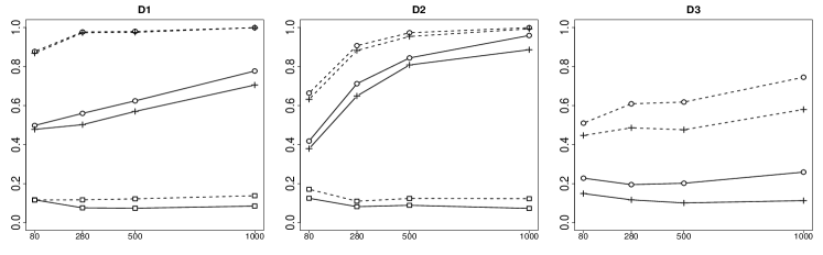
(a) Covariance structure M1

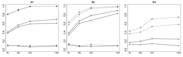
(b) Covariance structure M2

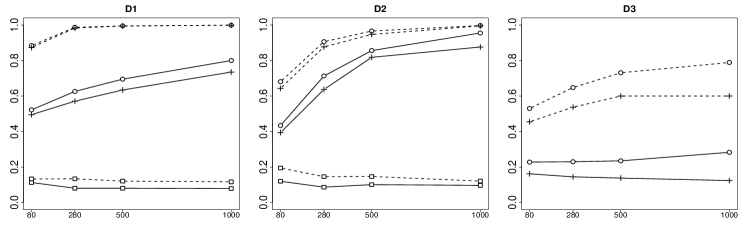
(c) Covariance structure M3

Figure 1: Comparison of empirical powers for data generated by data models D1–D3 with different covariance structures. In each panel, horizontal and vertical axes depict dimension $p$ and empirical powers, respectively; and unbroken lines and dashed lines represent the results for $(n_{1},n_{2})=(45,45)$ and $(60,80)$, respectively. The different symbols on the lines represent different tests experimented in the study, where $\circ$, $\oblong$, and $+$ indicate the proposed test, tests by Li and Chen (2012) and Cai et al. (2013), respectively. Results are based on 1000 replications with $\alpha=0.05$.

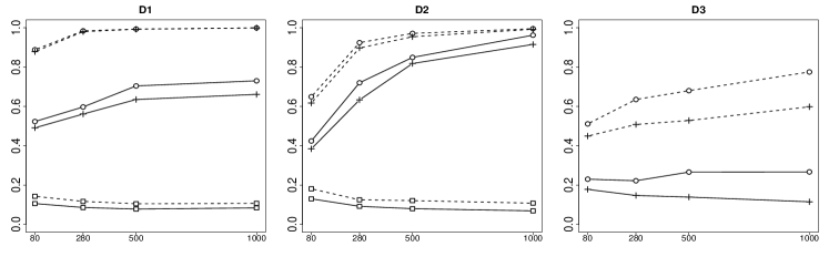
(d) Covariance structure M4

Figure 1(c) displays empirical power comparisons. We see that the proposed test $\Psi_{B,\alpha}$ and the CLX test are substantially more powerful than the LC test against sparse alternatives for the Gamma and zero-inflated Poisson data (data models D1 and D2) under different covariance structures. As the number of non-zero entries of $\boldsymbol{\Sigma}_{1}-\boldsymbol{\Sigma}_{2}$ grows in $p$, both the proposed test $\Psi_{B,\alpha}$ and the CLX test gain powers while the LC test do not gain much due to the sparsity of $\boldsymbol{\Sigma}_{1}-\boldsymbol{\Sigma}_{2}$. For the Gamma and zero-inflated Poisson data, the proposed test is slightly more powerful than the CLX test when the sample size is small and the two tests are closely comparable as the sample size increasing. For $t$-distributed data (data model D3), $\Psi_{B,\alpha}$ is more powerful than the CLX test and gains more powers along increasing sample sizes and dimensions. In summary, $\Psi_{B,\alpha}$ outperforms the other three for sparse alternatives of interest. More simulation results are reported in the supplementary material.

4 Application of the proposed procedure in gene clustering

The primary goal of gene clustering is to group genes with similar expression patterns together, which usually provides insights on their biological functions or regulatory pathways. In genomic studies, gene clustering has been employed for detecting co-expression gene sets (D’haeseleer, 2005; Sharan et al., 2002), identifying functionally related genes (Yi et al., 2007), and discovering large groups of genes suggestive of co-regulation by common factors, among other applications.

Consider a random sample $\mathcal{X}_{n}=\{{\mathbf{X}}_{1},\ldots,{\mathbf{X}}_{n}\}$ of $n$ independent observations from ${\mathbf{X}}=(X_{1},\ldots,X_{p})^{{\mathrm{\scriptscriptstyle T}}}$ with covariance $\boldsymbol{\Sigma}_{1}=(\sigma_{1,k\ell})_{1\leq k,\ell\leq p}$ and correlation ${\mathbf{R}}_{1}=(\rho_{1,k\ell})_{1\leq k,\ell\leq p}$, where ${\mathbf{X}}_{i}$ records the expression levels of $p$ genes from subject $i$. To cluster the genes based on their expression levels, some dissimilarity or proximity measure for the $p$ genes, or equivalently, the $p$ variables, is calculated based on $\mathcal{X}_{n}$, to which clustering algorithms are applied. Gene clustering can therefore be achieved via clustering the variables. To discover the clustering structure of variables, it is intuitive that variables $X_{k}$ and $X_{\ell}$ will be clustered in the same group if $|\rho_{1,k\ell}|$ is large and separated otherwise (Wagaman and Levina, 2009). Specifically, if there are some clustering structures among variables, then there exists a partition of $\{1,\ldots,p\}$ upon potential permutations, denoted by $\{B_{t}\}_{t=1}^{m}$ for some $1\leq m\leq p$, such that $\min_{k,\ell\in B_{t}}|\rho_{1,k\ell}|>c_{1}$, and for any $1\leq t\neq t^{\prime}\leq m$, $\max_{k\in B_{t},\ell\in B_{t^{\prime}}}|\rho_{1,k\ell}|<c_{2}$, where $c_{1},c_{2}>0$ are positive constants. The problem is then closely related to testing one-sample hypotheses that for a given $\Lambda\subseteq\mathcal{I}_{p}=\{(1,1),\ldots,(1,p),(2,1),\ldots,(2,p),\ldots,(p,p)\}$, $H_{0}^{\Lambda}:\rho_{1,k\ell}=0~{}\text{for any}~{}(k,\ell)\in\Lambda$ versus $H_{1}^{\Lambda}:\rho_{1,k\ell}\neq 0~{}\text{for some}~{}(k,\ell)\in\Lambda$, which is equivalent to

$$H_{0}^{\Lambda}:{\sigma_{1,k\ell}}=0~{}\text{for any}~{}(k,\ell)\in\Lambda\quad\mbox{versus}\quad H_{1}^{\Lambda}:{\sigma_{1,k\ell}}\neq 0~{}\text{for some}~{}(k,\ell)\in\Lambda.$$ (4.1)

Testing the hypothesis (4.1) facilitates recovering the dissimilarity patterns among variables; that is, failing to reject $H_{0}^{\Lambda}$ indicates the segregation between $X_{k}$ and $X_{\ell}$ whenever $(k,\ell)\in\Lambda$.

Motivated by the block-wise estimation method of Caragea and Smith (2007), we define $\Lambda$ in the following way. First, we place the covariance matrix $\boldsymbol{\Sigma}_{1}$ on a $p\times p$ grid indexed by $\mathcal{I}_{p}$ and partition it with blocks of moderate size. Due to symmetry, we only focus on the upper triangle part. Second, we construct blocks of size $s_{0}\times s_{0}$ along the diagonal and note that the last block may be of a smaller size if $s_{0}$ is not a divisor of $p$. Next, we create new blocks of size $s_{0}\times s_{0}$ successively toward the top right corner. Similarly as before, blocks to the most right may be of smaller size. The grid, or equivalently, the index set $\mathcal{I}_{p}$, is partitioned into $S=\lceil p/s_{0}\rceil(\lceil p/s_{0}\rceil+1)/2$ sub-regions and we denote by $\Lambda_{1},\ldots,\Lambda_{S}$ the partition of the upper triangle indices $\{(k,\ell):1\leq k<\ell\leq p\}$.

On each of the sub-regions, we modify the proposed procedure for testing local hypotheses $H_{0}^{\Lambda_{s}}:\sigma_{1,k\ell}=0$ for any $(k,\ell)\in\Lambda_{s}$ versus $H_{1}^{\Lambda_{s}}:\sigma_{1,k\ell}\neq 0$ for some $(k,\ell)\in\Lambda_{s}$, $s=1,\ldots,S$. We then apply the Benjamini-Hochberg (BH) procedure to control the false discovery rate (FDR) for simultaneously testing $S$ hypotheses. For each $s$, failing to reject the null $H_{0}^{\Lambda_{s}}$ indicates a segregation between $X_{k}$ and $X_{\ell}$ for $(k,\ell)\in\Lambda_{s}$ and zero will be assigned as the similarity between $X_{k}$ and $X_{\ell}$. We summarize this procedure as follows.

(I) Compute the sample covariance matrix $\widehat{\boldsymbol{\Sigma}}_{1}=(\hat{\sigma}_{1,k\ell})_{1\leq k,\ell\leq p}$ and $\widehat{\mathbf{T}}=(\tilde{t}_{k\ell})_{1\leq k,\ell\leq p}$, where $\tilde{t}_{k\ell}=n^{1/2}\hat{s}_{1,k\ell}^{-1/2}\hat{\sigma}_{1,k\ell}$ for $\hat{s}_{1,k\ell}$ defined in Section (2.2).

(II) Independent of $\mathcal{X}_{n}$, simulate a sample of size $B$, where for each $b=1,\ldots,B$ and $1\leq k\leq\ell\leq p$, compute $\tilde{t}^{\,\dagger}_{b,k\ell}=(n^{-1}\hat{s}_{1,k\ell})^{-1/2}\sum_{i=1}^{n}g_{b,i}\{(X_{ik}-\bar{X}_{k})(X_{i\ell}-\bar{X}_{\ell})-\hat{\sigma}_{1,k\ell}\},$ where $\{g_{b,1},\ldots,g_{b,n}\}$ is a sequence of i.i.d. standard normal random variables.

(III) Partition the $p\times p$ grid as discussed before by $S$ blocks. For each block with entries indexed by $\Lambda_{s}\subset\mathcal{I}_{p}$, compute the approximated $p$-value as $\hat{p}_{s}=1-\widehat{F}_{B}\left(\max_{(k,\ell)\in\Lambda_{s}}\tilde{t}_{k\ell}\right),$ where $\widehat{F}_{B}$ denotes the empirical (conditional) distribution function of $\max_{(k,\ell)\in\Lambda_{s}}\tilde{t}_{k\ell}$ given $\mathcal{X}_{n}$ using the simulated samples $\{\max_{(k,\ell)\in\Lambda_{s}}\tilde{t}^{\,\dagger}_{b,k\ell}\}_{b=1}^{B}$.

(IV) Estimate the $q$-values for $\{\hat{p}_{s}\}_{s=1}^{S}$ using the BH procedure, denoted by $\{\hat{q}_{s}\}$. For a prespecified cut-off $\pi$, define the dissimilarity measure by

$$d_{k\ell}=1-\frac{\tilde{t}_{k\ell}I(\hat{q}_{s}<\pi)}{\max\{\max_{(k,\ell)\in\Lambda_{s}}\tilde{t}_{k\ell},1\}}~{}~{}~{}\textrm{for any}~{}~{}(k,\ell)\in\Lambda_{s}.$$ (4.2)

Based on the measure in (4.2), we can apply clustering algorithms such as the hierarchical clustering for clustering variables and obtain gene clustering. To specify the blocks, we propose the following data-driven selection of $s_{0}$. The $S$ local hypotheses to be tested simultaneously admit unknown complex dependencies so that the FDR, controlled by the BH procedure, satisfies the general upper bound ${\rm FDR}\leq(\pi S_{0}\log S)/S$ where $S_{0}$ denotes the number of true null local hypotheses (Benjamini and Yekutieli, 2001). To control the FDR at the nominal level $\pi$, we need $S\geq S_{0}\log S$ which is automatically satisfied when $S=1$ or $s_{0}$ is large. Therefore, we define a data-driven $s_{0}$ by $s_{0}=\max\{\lceil\log p\rceil,\min(s:\widehat{S}_{0}(s)\leq S(s)[\log\{S(s)\}]^{-1})\}$, where $S(s)=\lceil p/s\rceil(\lceil p/s\rceil+1)/2$ and $\widehat{S}_{0}$ is an estimate for the number of true null local hypotheses. In practice, we may also reorder the variables first using methods such as the Isoband algorithm by Wagaman and Levina (2009). A demonstration of the proposed clustering algorithm, as well as comparisons of $d_{k\ell}$ with traditional dissimilarity measures based on the human asthma data, is displayed in the Supplementary Materials.

5 Application to analysis of human asthma data

5.1 Background

As a common chronic inflammatory disease of the airways, asthma is caused by a combination of complex genetic and environmental interactions and affects more than 200 million people worldwide as of 2013 as shown in 2013 World Health Organization Fact Sheet No. 307. The mechanism and regulatory pathways remain unclear. We illustrate the proposed new procedures using the human asthma data from the microarray experiment reported by Voraphani et al. (2014), which was aimed to understand the regulatory pathway and mechanism for high nitrative stress, a major characteristic of human severe asthma. Voraphani et al. (2014) identified several novel pathways, including discovering that the Th1 cytokine, IFN-$\gamma$, along or with Th2 regulations, are critical immune agents for the disease development by amplifying epithelial NAD/NADPH thyroid oxidase expression and aiding the production of nitrite.

The original microarray gene expression data are available at the NCBI’s Gene Expression Omnibus database with the Gene Expression Omnibus Series accession number GSE43696. The data consist of $n_{1}=20$ health samples and $n_{2}=88$ patients suffering from moderate or severe asthmatics. We focused on identifying disease-associated GO terms. After preliminary filtering steps using the approach in Gentleman et al. (2005) and removing genes without appropriate annotations, there remained $24,520$ genes. We excluded GO terms with missing information or less than 10 genes. There retained $3,290$ GO terms from the original dataset whose sizes vary from 11 to $8,070$ genes. For $g=1,\ldots,G$ with $G=3,290$, denote by $\boldsymbol{\mu}_{h,g}$ and $\boldsymbol{\mu}_{a,g}$ the mean gene expression levels, and $\boldsymbol{\Sigma}_{h,g}$ and $\boldsymbol{\Sigma}_{a,g}$ the covariance matrices for the $g^{\text{th}}$ GO term in the control and disease groups, respectively.

5.2 Differential expression analysis

A commonly used method in differential analysis is the mean-based test that selects interesting GO terms by testing the null hypothesis that overall gene expressions within a GO term are similar across populations (Chen and Qin, 2010; Chang et al., 2014; Wang et al., 2015). Though the mean-based procedure has been successful in detecting differential expressed genes based on the changes in the expression level, recent developments in genomic analysis have revealed the importance to detect genes with changing relationships with other genes in different biological states, and particularly GO terms that change the dependence structures across populations (de la Fuente, 2010). The discovery of those GO terms with altered dependence structures provides information on critical gene regulation pathways. Consider all the GO terms, we applied the proposed method $\Psi_{B,\alpha}$ to test the global hypotheses

$$H^{c}_{0g}:\boldsymbol{\Sigma}_{h,g}=\boldsymbol{\Sigma}_{a,g}\quad\mbox{versus}\quad H^{c}_{1g}:\boldsymbol{\Sigma}_{h,g}\neq\boldsymbol{\Sigma}_{a,g}.$$ (5.1)

For a comparison, we also applied the LC and CLX tests.

Here, $B=5,000$ Monte Carlo replications were employed to compute the $p$-values for $\Psi_{B,\alpha}$. By controlling the FDR at $2.5\%$ (Benjamini and Yekutieli, 2001), the proposed test $\Psi_{B,\alpha}$ declared 969 GO terms significant while the LC and CLX tests declared 290 and 524 GO terms significant, respectively. The proposed test $\Psi_{B,\alpha}$ has found more significant GO terms and is less conservative than the others, which is also reflected by the histograms of $p$-values for the three tests displayed in the Supplementary Material. Table 3 displays the top 15 most significant GO terms declared by $\Psi_{B,\alpha}$ and also highlights those GO terms that were not detected by the LC and CLX tests. For example, GO:0005887 (integral to plasma membrane) is functionally relevant to the dual oxidases (DUOX2)-thyroid peroxidase interaction and is important to the mechanism of asthma development (Voraphani et al., 2014). It is worth noticing that $\Psi_{B,\alpha}$ is able to discover this biologically important GO term that is missed by the others. This further highlights the good performance of our proposed test.

Table 3: Top 15 most significant GO terms detected by $\Psi_{B,\alpha}$ with FDR controlled at $2.5\%$, $\flat$ and ${\dagger}$ refer to the GO terms not being declared significant by the CLX test and the LC test, respectively.

GO ID	GO term name
GO:0006886	intracellular protein transport †
GO:0008565	protein transporter activity †
GO:0030117	membrane coat †
GO:0005515	protein binding♭,†
GO:0016032	viral reproduction♭,†
GO:0005829	cytosol†
GO:0000278	mitotic cell cycle†
GO:0006334	nucleosome assembly†
GO:0034080	CenH3-containing nucleosome assembly at centromere
GO:0006974	response to DNA damage stimulus†
GO:0016874	ligase activity†
GO:0032007	negative regulation of TOR signaling cascade†
GO:0005887	integral to plasma membrane♭,†
GO:0006997	nucleus organization†
GO:0030154	cell differentiation†

In addition, we compared the study on changing intergene relationships across biological states with the traditional differential analysis based on mean expression levels. The proposed test on intergene relationships discovered 268 significant GO terms that were missed by the traditional differential analysis. This reflects the lately growing demands on analyzing gene dependence structures. More details on this comparison are retained in the supplement.

5.3 Gene clustering study on GO terms of interest

Voraphani et al. (2014) revealed a novel pathway involving epithelial iNOS, dual oxidases, TPO and the cytokine INF-$\gamma$ to understand the mechanism of human asthma. Multiple transcripts, together with their variants, are related, while their co-regulation mechanisms are less clear. The proposed gene clustering algorithm provides a way to study gene interactions.

For illustration, we focus on the GO terms that were declared significant via testing (5.1) and are related to IFN-$\gamma$ or TPO, and apply our clustering procedure to the sample from the health and disease groups separately to study how the gene clustering alters across two populations. For IFN-$\gamma$, we consider the GO terms 0032689 (negative regulation of IFN-$\gamma$ production), 0060333 (IFN-$\gamma$-mediated signaling pathway) and 0071346 (cellular response to IFN-$\gamma$). For TPO, the GO terms have been considered include 0004601 (peroxidase activity), 0042446 (hormone biosynthetic process), 0035162 (embryonic hemopoiesis), 0006979 (response to oxidative stress), and 0009986 (cell surface). Their sizes vary from 17 to 439.

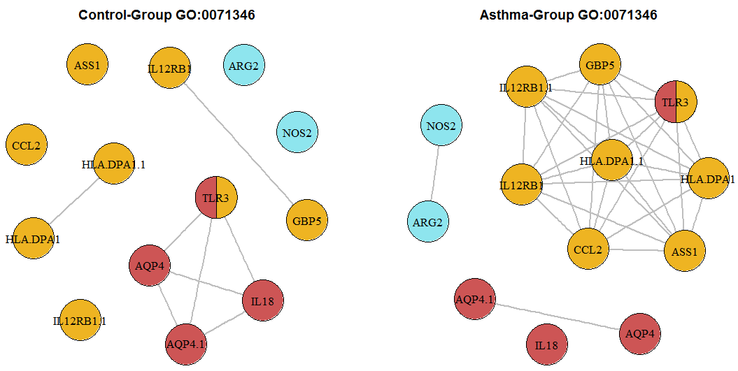
(a) GO:0071346, cellular response to INF-$\gamma$

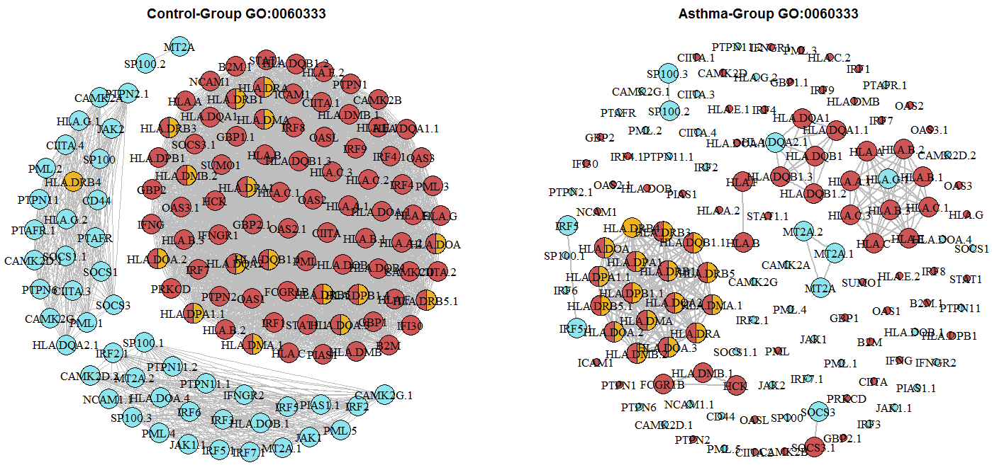
(b) GO:0060333, INF-$\gamma$-mediated signaling pathway

Figure 2: Comparison of clustering structures of GO:0071346, cellular response to INF-$\gamma$ and GO:0060333, INF-$\gamma$-mediated signaling pathway, between health and disease groups using the proposed gene clustering procedure. This figure appears in color in the electronic version of this article.

We take $B=5,000$, $\alpha=0.05$ and use hierarchical clustering algorithm with average linkage. The $\widehat{S}_{0}$ is estimated using the censored Beta-Uniform mixture model by Markitsis and Lai (2010) for selecting block size $s_{0}$. Figures 2–3 display comparisons of gene clustering between the health and disease groups (more comparisons are included in the Supplementary Material). Each vertex in the figures represents a gene or its variant and is labelled by the corresponding ID. Vertexes connected by edges in gray are clustered into one group, and vertexes in red and yellow belong respectively to the maximum clique in the health and disease groups. Vertexes in both colors belong to the maximum cliques for both groups.

From Figure 2 we see that for GO:0071346, regarding the cellular response to INF-$\gamma$, genes tend to function more in clusters in the asthma group than those in the health group. Gene TLR3 actively appears in the largest gene clusters for both the health and asthma groups, while gene IL18 is isolated in the asthma group. Gene NOS2 is involved in asthma by co-regulating with ARG2. These suggest that these four genes are important signatures for understanding the effect of INF-$\gamma$ on the asthma progression. Regarding the INF-$\gamma$-mediated signaling pathway, Figure 2 also shows that compared to the health group, genes seem to preferentially function separately in the asthma group. The original dominating gene clusters are broken into small groups in the presence of the disease. The different configurations in primary gene clusters between the health and asthma groups for GO:0060333 provide further information on how INF-$\gamma$ influences the iNOS pathway. For the critical enzyme TPO, Figure 3 shows that genes also tend to function in clusters in the disease group. In the presence of asthma, the gene cluster HBB-HBA2.1-HBA2 is preserved and the gene IPCEF1 is isolated from the original largest gene cluster for GO:0004601. It is interesting to notice that the DUOX2 genes are isolated in the health group but do interact with many genes, particularly with TPO, in the presence of asthma as documented in Voraphani et al. (2014). The identified DUOX2 gene cluster provides a candidate pathway to understand how TPO catalyzes the iNOS-DUOX2-thyroid peroxidase pathway discovered by Voraphani et al. (2014). Last but not least, it can be seen from Figure 3 that the overall co-regulation patterns remain similar across populations, while those of TPO alters in the presence of asthma.

In summary, based on the proposed procedure, not only can we test the difference in gene dependence, we can also discover the disparity in gene clustering, which reflects the difference in gene clustering patterns between the health and disease groups.

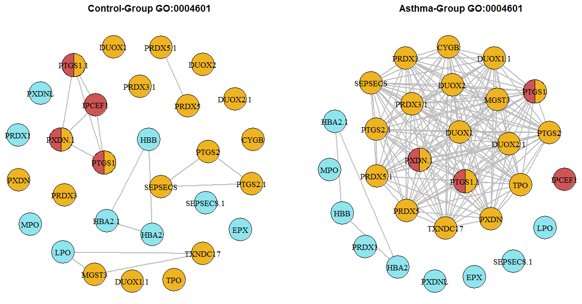
(a) GO:0004601, peroxidase activity

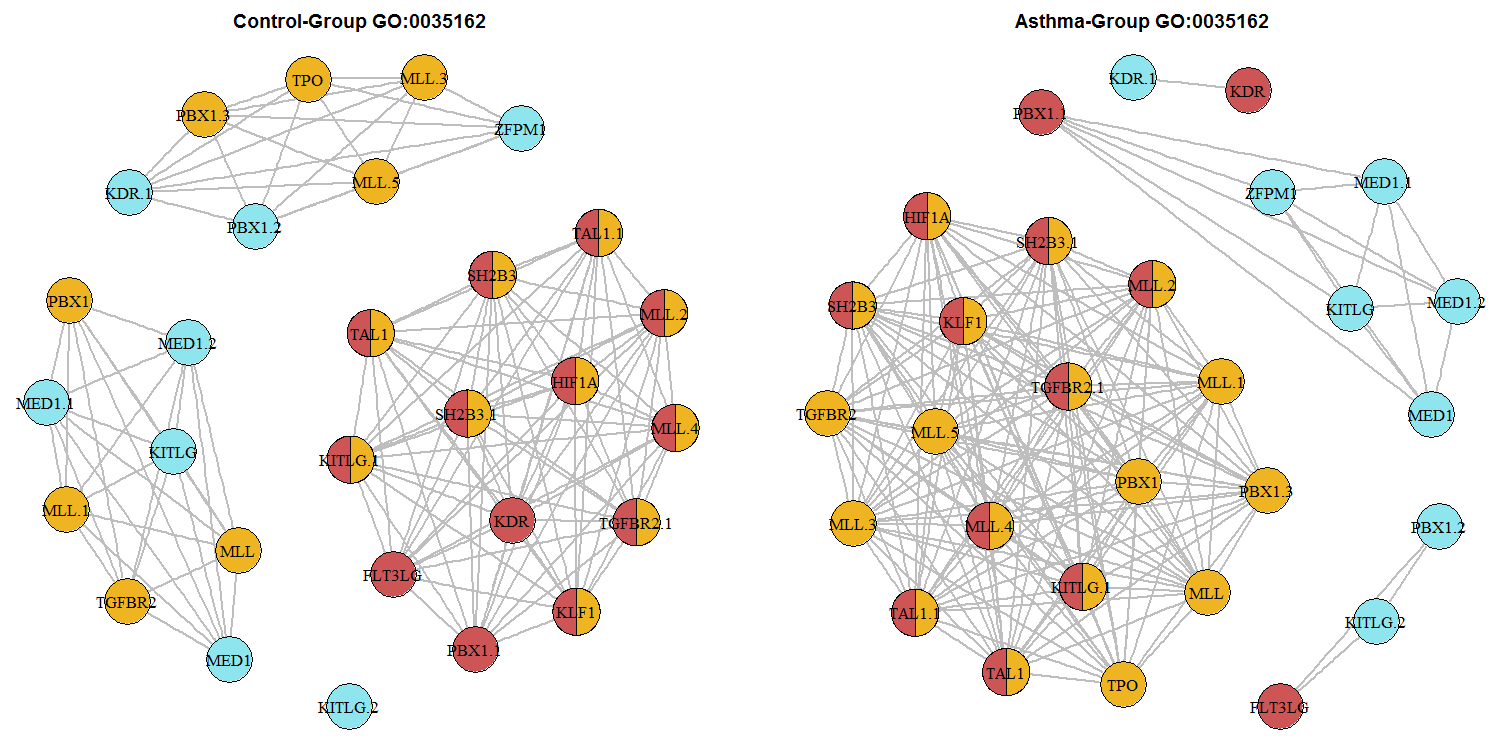
(b) GO:0035162, embryonic hemopoiesis

Figure 3: Comparison of clustering structures of GO:0004601, peroxidase activity and GO:0035162, embryonic hemopoiesis, between health and disease groups using the proposed gene clustering procedure. This figure appears in color in the electronic version of this article.

6 Conclusion and discussion

In this paper, we proposed a computationally fast and effective procedure for testing the equality of two large covariance matrices. The proposed procedure is powerful against sparse alternatives corresponding to the situation where the two covariance matrices differ only in a small fraction of entries. Compared to existing tests, the proposed procedure requires no structural assumptions on the unknown covariance matrices and remains valid under mild conditions. These appealing features grant the proposed test a vast applicability, particularly for real problems arising in genomics. As an important application, we introduced a gene clustering algorithm that enjoys the same nice feature of avoiding imposing structural assumptions on the unknown covariance matrices.

Another interesting and related problem is testing the equality of two precision matrices, which was recently studied by Xia et al. (2015). In the literature of graphical models, it is common to impose the Gaussian assumption on data so that the conditional dependency can be inferred based on the precision matrix. When the discrepancy between two precision matrices is believed to be sparse, the data-dependent procedure considered in this paper can be extended to comparing them by utilizing the similar $L_{\infty}$-type statistic discussed in Xia et al. (2015). It is interesting to investigate whether our method can be applied to testing precision matrices in the presence of heavy-tailed data, which is often modeled by the elliptical distribution family. We leave this to future work.

7 Supplementary Materials

Web Appendices, which include proofs of the main theorems and additional numerical results referenced in Sections 2, 3 and 5 are available with this paper on the Biometrics website on Wiley Online Library.

References

- Anderson (2003) Anderson, T. W. (2003). An Introduction to Multivariate Statistical Analysis. 3rd edition. New York: Wiley-Interscience.
- Benjamini and Yekutieli (2001) Benjamini, Y. and Yekutieli, D. (2001). The control of the false discovery rate in multiple testing under dependency. The Annals of Statistics 29, 1165–1188.
- Cai et al. (2013) Cai, T. T., Liu, W., and Xia, Y. (2013). Two-sample covariance matrix testing and support recovery in high-dimensional and sparse settings. Journal of the American Statistical Association 108, 265–277.
- Caragea and Smith (2007) Caragea, P. and Smith, R. (2007). Asymptotic properties of computationally efficient alternative estimators for a class of multivariate normal models. Journal of Multivariate Analysis 98, 1417–1440.
- Chang et al. (2014) Chang, J., Zhou, W., and Zhou, W.-X. (2014). Simulation-based hypothesis testing of high dimensional means under covariance heterogeneity. Available at arXiv:1406.1939.
- Chen and Qin (2010) Chen, S. X. and Qin, Y. (2010). A two-sample test for high-dimensional data with applications to gene-set testing. The Annals of Statistics 38, 808–835.
- Chernozhukov et al. (2013) Chernozhukov, V., Chetverikov, D., and Kato, K. (2013). Gaussian approximations and multiplier bootstrap for maxima of sums of high-dimensional random vectors. The Annals of Statistics 41, 2786–2819.
- de la Fuente (2010) de la Fuente, A. (2010). From differential expression to differential networking – identification of dysfunctional regulatory networks in diseases. Trends in Genetics 26, 326–333.
- D’haeseleer (2005) D’haeseleer, P. (2005). How does gene expression clustering work? Nature Biotechnology 23, 1499–1501.
- Gentleman et al. (2005) Gentleman, R., Irizarry, R. A., Carey, V. J., Dudoit, S., and Huber, W. (2005). Bioinformtics and Computational Biology Solutions Using R and Bioconductor. New York: Springer-Verlag.
- Katsani et al. (2014) Katsani, K. R., Irimia, M., Karapiperis, C., Scouras, Z. G., Blencowe, B. J., Promponas, V. J., and Ouzounis, C. A. (2014). Functional genomics evidence unearths new moonlighting roles of outer ring coat nucleoporins. Scientific Reports 4, 4655.
- Li and Chen (2012) Li, J. and Chen, S. X. (2012). Two-sample tests for high-dimensional covariance matrices. The Annals of Statistics 40, 908–940.
- Liu et al. (2008) Liu, W., Lin, Z. Y. and Shao, Q.-M. (2008). The asymptotic distribution and Berry-Esseen bound of a new test for independence in high dimension with an application to stochastic optimization. The Annals of Applied Probability 18, 2337–2366.
- Markitsis and Lai (2010) Markitsis, A. and Lai, Y. (2010). A censored beta mixture model for the estimation of the proportion of non-differentially expressed genes. Bioinformatics 26, 640–646.
- Schott (2007) Schott, J. R. (2007). A test for the equality of covariance matrices when the dimension is large relative to the sample size. Computational Statistics and Data Analysis 51, 6535–6542.
- Sharan et al. (2002) Sharan, R., Elkon, R., and Shamir, R. (2012). Cluster analysis and its applications to gene expression data. Ernst Schering Research Foundation Workshop 38, 83–108.
- Srivastava and Yanagihara (2010) Srivastava, M. S. and Yanagihara, H. (2010). Testing the equality of several covariance matrices with fewer observations than the dimension. Journal of Multivariate Analysis 101, 1319–1329.
- van der Vaart and Wellner (1996) van der Vaart, A. W. and Wellner, J. A. (1996). Weak Convergence and Empirical Processes: With Applications to Statistics. New York: Springer.
- Voraphani et al. (2014) Voraphani, N., Gladwin, M. T., Contreras, A. U., Kaminski, N., Tedrow, J. R., Milosevic, J., Bleecker, E. R., Meyers, D. A., Ray, A., Ray, P., Erzurum, S. C., Busse, W. W., Zhao, J., Trudeau, J. B., and Wenzel, S. E. (2014). An airway epithelial iNOS-DUOX2-thyroid peroxidase metabolome drives Th1/Th2 nitrative stress in human severe asthma. Mucosal Immunology 7, 1175–1185.
- Wolen and Miles (2012) Wolen, A. R. and Miles, M. F. (2012). Identifying gene networks underlying the neurobiology of ethanol and alcoholism. Alcohol Research: Current Reviews 34, 306–317.
- Wagaman and Levina (2009) Wagaman, A. S. and Levina, E. (2009). Discovering sparse covariance structures with the Isomap. Journal of Computational and Graphical Statistics 18, 551–572.
- Wang et al. (2015) Wang, L., Peng, B., and Li., R. (2015). A high-dimensional nonparametric multivariate test for mean vector. Journal of the American Statistical Association 110, 1658–1669.
- Xia et al. (2015) Xia, Y., Cai, T., and Cai, T. T. (2015). Testing differential networks with applications to the detection of gene-gene interactions. Biometrika 94, 247–266.
- Yi et al. (2007) Yi, G., Sze, S.-H., and Thon, M. (2007). Identifying clusters of functionally related genes in genomes. Bioinformatics 23, 1053–1060.