On a spatial-Temporal Decomposition of Optical Flow

Abstract

In this paper we present a decomposition algorithm for computation of the spatial-temporal optical flow of a dynamic image sequence. We consider several applications, such as the extraction of temporal motion features and motion detection in dynamic sequences under varying illumination conditions, such as they appear for instance in psychological flickering experiments. For the numerical implementation we are solving an integro-differential equation by a fixed point iteration. For comparison purposes we use a standard time dependent optical flow algorithm, which in contrast to our method, constitutes in solving a spatial-temporal differential equation.

Aniello Raffaele Patrone^∗

Computational Science Center

University of Vienna

Oskar-Morgenstern Platz 1, 1090 Vienna, Austria

Otmar Scherzer

Computational Science Center

University of Vienna

Oskar-Morgenstern Platz 1, 1090 Vienna, Austria

and

Johann Radon Institute for Computational and Applied Mathematics

(RICAM)

Altenbergerstraße 69, 4040 Linz, Austria

1 Introduction

Analyzing the motion in a dynamic sequence is of interest in many fields of applications, like human computer interaction, medical imaging, psychology, to mention but a few. In this paper we study the extraction of motion in dynamic sequences by means of the optical flow, which is the apparent motion of objects, surfaces, and edges in a dynamic visual scene caused by the relative motion between an observer and the scene. There have been proposed several computational approaches for optical flow computations in the literature. In this paper we emphasize on variational methods. In this research area the first method is due to Horn & Schunck [15]. Like many alternatives and generalizations, the Horn & Schunck method calculates the flow from two consecutive frames. Here, we are calculating the optical flow from all available frames simultaneously. Spatial-temporal optical flow methods were previously studied by Weickert & Schnörr [28, 29], [11], [26] and [2], to name but a few. However, in contrast to these paper we emphasize on a decomposition of the optical flow into components, instead of calculating the flow itself.

Variational modeling of patterns in stationary images has been initialized with the seminal book of Y. Meyer [20]. In the context of total variation regularization, reconstructions of patterns was studied first in [24]. Here, we are implementing similar ideas as have been used before for variational image denoising [3, 4, 5, 6, 7, 13, 25] and optical flow decomposition [1, 18, 30, 31, 32]. However, a conceptual difference is that we aim for extracting temporal features, while, in all the cited papers the decomposition was for finding spatial components of the flow. We emphasize that the proposed method is one of very few variational optical flow algorithms in a space-time regime and within this class, this algorithm is the only spatial-temporal decomposition algorithm.

The outline of this paper is as follows: In Section 2 we review the optical flow equation. In Section 3 we present analytical examples of the optical flow equation in case of illumination changes. In Section 4 we introduce the new model for spatial-temporal optical flow decomposition. We formulate it as a minimization problem and derive the optimality conditions for a minimizer. In Section 5 we derive a fixed point algorithm for numerical minimization of the energy functional. Finally in Section 6 and Section 7 we present experiments, results and a discussion of them.

2 Registration and optical flow

The problem of aligning dynamic sequences $f(\cdot,t)$, $t\in(0,1)$ can be formulated as the operator equation for finding a flow $\Psi$ of diffeomorphisms,

$$\Psi(\cdot,t):\Omega\to\Omega,\quad\forall\,t\in(0,1),$$

such that

$$f(\Psi(\vec{x},t),t)=f(\vec{x},0),\qquad\forall\,\vec{x}\in\Omega\text{ and }t\in(0,1).$$ (1)

For the sake of simplicity of presentation we consider the time interval as the unit interval all along the paper.

Differentiation of (1) with respect to $t$ for a fixed $\vec{x}$ gives

$$\nabla f(\Psi(\vec{x},t),t)\cdot\partial_{t}\Psi(\vec{x},t)+\partial_{t}f(\Psi(\vec{x},t),t)=0,\qquad\forall\,\vec{x}\in\Omega\text{ and }t\in(0,1).$$ (2)

Switching from a Lagrangian to an Eulerian description we obtain the optical flow equation (OFE) on $\Omega$:

$$\nabla f(\vec{x},t)\cdot\vec{u}(\vec{x},t)+\partial_{t}f(\vec{x},t)=0,\qquad\forall\,\vec{x}\in\Omega\text{ and }t\in(0,1).$$ (3)

Although the derivation is based on a constant brightness assumption along characteristics, mathematically, (3) even makes sense under varying illumination conditions. However, as we show in simple examples below, standard regularity assumptions on the optical flow are violated when the characteristics degenerate (collapse or originate) or when the illumination changes. Instead of solving (3) usually the relaxed problem is considered, which consists in minimizing the functional

$$\text{argmin }S(\vec{u}):=\int_{\Omega}(\nabla f(\vec{x},t)\cdot\vec{u}(\vec{x},t)+\partial_{t}f(\vec{x},t))^{2}\,\mathrm{d}\vec{x}\,,\qquad\forall t\in(0,1),$$ (4)

subject to appropriate constraints.

3 The optical flow equation in case of illumination changes

In this section we are providing simple motivating examples explaining properties of the solution of the optical flow equation (3) under changing illumination conditions. Here we are restricting attention to a spatial domain $\emptyset\neq\Omega=(0,1)\subset\mathbbm{R}$.

The following two examples simulate a day to night illumination situation. The optical flow is calculated analytically, and the level lines of $f$ are visualized, which represent the trajectories $\Psi$ of constant brightness. As we show, smoothness of the optical flow is affected by changing illumination and in the first example also by joining of characteristic curves.

Example 1.

In this example the flow is not even an element of the Bochner-space $L^{2}((0,1);H^{-1}(\Omega))$, meaning that the anti-derivative of $u$ with respect to time is not in $L^{2}((0,1);L^{2}(\Omega))$. Because $L^{2}((0,1);H^{-1}(\Omega))$ is a strict superset of $L^{2}((0,1);L^{2}(\Omega))$, the elements have in general less regularity (smoothness). The next Example 2 provides a flow where $f$ models again changing illumination. Here the flow is in $L^{2}((0,1);H^{-1}(\Omega))$ but not in $L^{2}((0,1);L^{2}(\Omega))$. We conjecture from the difference of the two examples that the difference in smoothness is caused by the fact that in the first example two characteristics are joining during the evolution.

We consider the 1D optical flow equation, to solve for $u$ in

$$\partial_{x}f(x,t)u(x,t)+\partial_{t}f(x,t)=0,\quad\forall(x,t)\in(0,1)\times(0,1)$$ (5)

for the specific data

$$f(x,t)=\tilde{f}(x)g(t),\quad\forall(x,t)\in(0,1)\times(0,1).$$ (6)

$f$ represents a static scene $\tilde{f}$, which is affected by brightness variations over time, described by $g$. We are more specific and take:

$$\tilde{f}(x)=x(1-x)\text{ and }g(t)=1-t,\quad\forall(x,t)\in(0,1)\times(0,1).$$ (7)

The function $f$ and the level lines are plotted in Figure 1 and the optical flow can be calculated explicitly:

$$u(x,t)=\frac{x(1-x)}{1-2x}\frac{1}{1-t},\quad\forall(x,t)\in(0,1)\times(0,1),$$

indicates a transport of intensities from outside to the center $1/2$. We observe that $u(1/2,t)$ and $u(x,1)$ are singularities of the optical flow.

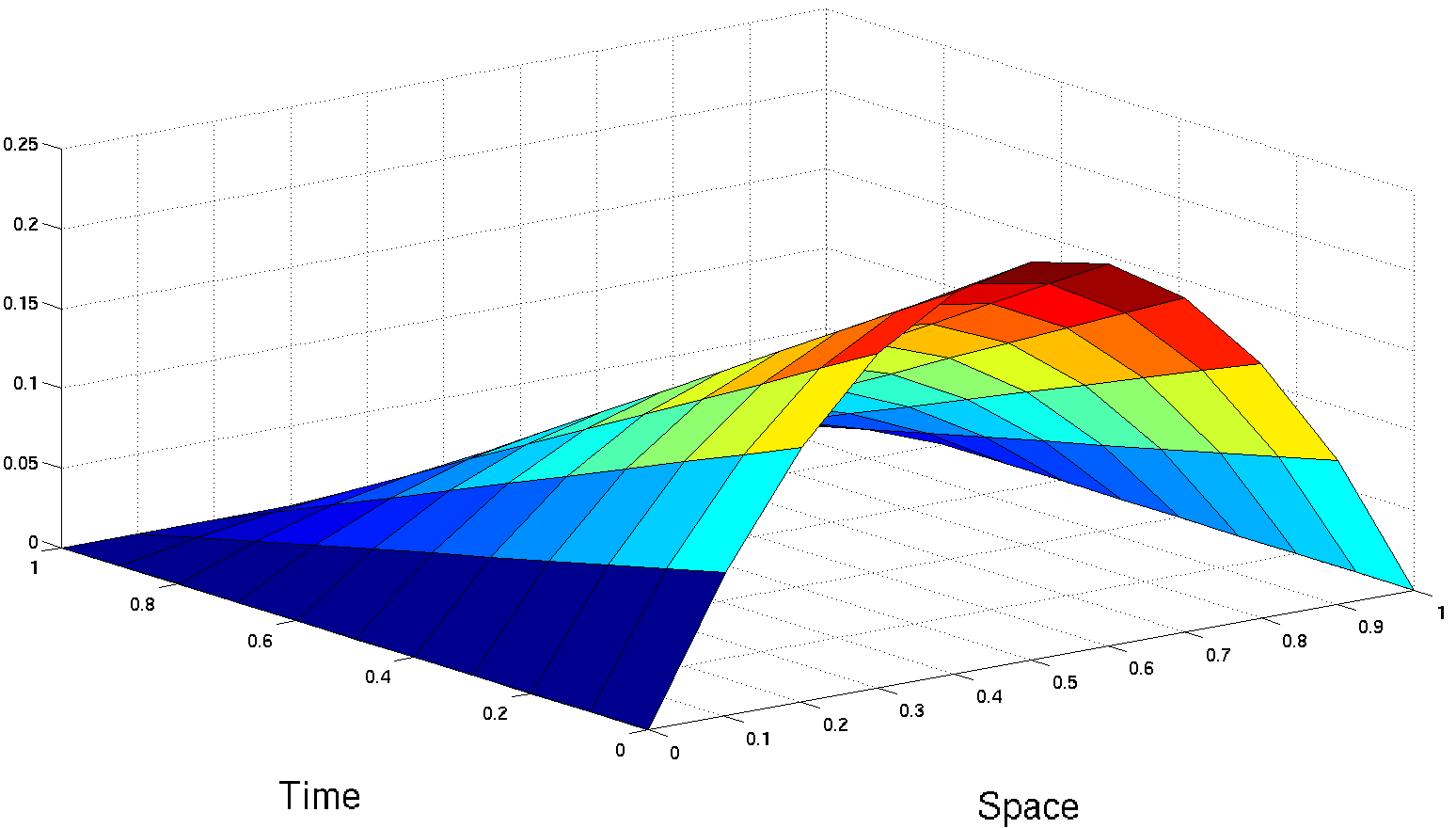
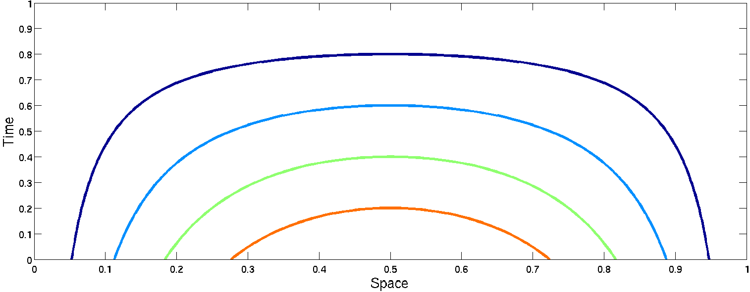
Figure 1: $f(x,t)=x(1-x)(1-t)$ from (7). Level lines of $f$ are parametrized by $(\Psi(x,t),t)$.

From the definition of $u$ it follows that

$$\hat{u}(x,t):=\int_{0}^{t}u(x,\tau)\,\mathrm{d}\tau=-\frac{x(1-x)}{1-2x}\log(1-t),\quad\forall(x,t)\in(0,1)\times(0,1)$$

and thus

$$\left\|\hat{u}\right\|_{L^{2}((0,1)^{2})}^{2}=\int_{0}^{1}\frac{x^{2}(1-x)^{2}}{(1-2x)^{2}}\,\mathrm{d}x\int_{0}^{1}\log^{2}(1-t)\,\mathrm{d}t\\ =2\int_{0}^{1}\frac{x^{2}(1-x)^{2}}{(1-2x)^{2}}\,\mathrm{d}x=\infty,$$

or in other words $\hat{u}\notin L^{2}((0,1)^{2})$.

Example 2.

This example is similar to Example 1, and simulates again a day to night illumination, with the difference that characteristics of $f$ never join. We consider input data $f$ of the form (6) with

$$\tilde{f}(x)=x(1-x)\text{ and }g(t)=\exp\left\{-\frac{1}{\beta}(1-t)^{\beta}\right\}\text{ with some }0<\beta<1$$ (8)

for $(x,t)\in\hat{\Omega}:=(0,1/4)\times(0,1)$. The optical flow is given by

$$u(x,t)=-\frac{x(1-x)}{1-2x}(1-t)^{\beta-1}.$$

Integrating this function over time gives

$$\hat{u}(x,t):=\int_{0}^{t}u(x,\tau)\,\mathrm{d}\tau=\frac{x(1-x)}{1-2x}\frac{1}{\beta}((1-t)^{\beta}-1),$$

Figure 2: $g(t)=\exp\left\{-\frac{1}{\beta}(1-t)^{\beta}\right\}$

and consequently with

$$C:=\int_{0}^{1/4}\frac{x^{2}(1-x)^{2}}{(1-2x)^{2}}\,\mathrm{d}x<\infty\,,$$

we get

$$\left\|u\right\|_{L^{2}(\hat{\Omega})}^{2} =C\int_{0}^{1}t^{2\beta-2}\,\mathrm{d}t=\left\{\begin{array}[]{rl}C\frac{1}{2\beta-1}&\text{ if }\beta>\frac{1}{2}\,,\\ \infty&\text{else}\;.\end{array}\right.$$

$$\left\|\hat{u}\right\|_{L^{2}(\hat{\Omega})}^{2} =\frac{C}{\beta^{2}}\int_{0}^{1}t^{2\beta}-2t^{\beta}+1\,\mathrm{d}t=\frac{C}{\beta^{2}}\left(\frac{1}{2\beta+1}-\frac{2}{\beta+1}+1\right) \text{ if }\beta>0\,.$$

This shows that $u\notin L^{2}(\hat{\Omega})$ for every $\beta\in(0,\frac{1}{2}]$, but $\hat{u}\in L^{2}(\hat{\Omega})$ for all $\beta\in(0,1)$.

The bottom line of these examples is that illumination changes, such as flickering, may result in singularities of the optical flow and a violation of standard smoothness assumptions of the optical flow (such as $\vec{u}\in L^{2}((0,1);H^{s}(\Omega))$ for some $s>0$). The potential appearance of the singularities motivates us to consider regularization terms for optical flow computations, which allow for singularities over time, such as negative Sobolev-norms.

4 Optical flow decomposition: basic setup and formalism

In this paper we derive an optical flow model which allows for decomposing the flow field into spatial and temporal components. We consider each frame of the movie $\left\{f(\cdot,t):t\in(0,1)\right\}$ defined on the two-dimensional spatial domain $\Omega=(0,1)^{2}$.

We assume that the optical flow field is a compound of two flow field components

$$\vec{u}(\vec{x},t)= \vec{u}^{(1)}(\vec{x},t)+\vec{u}^{(2)}(\vec{x},t)=\left(\begin{array}[]{c}u_{1}^{(1)}(\vec{x},t)\\ u_{2}^{(1)}(\vec{x},t)\end{array}\right)+\left(\begin{array}[]{c}u_{1}^{(2)}(\vec{x},t)\\ u_{2}^{(2)}(\vec{x},t)\end{array}\right),$$

$$\forall\vec{x}\in\Omega\text{ and }t\in(0,1).$$

Because there appears a series of indices and variables we specify the notation in Table 1.

$\vec{x}=(x_{1},x_{2})$	vector in two-dimensional Euclidean space
$\partial_{k}=\frac{\partial}{\partial x_{k}}$	differentiation with respect to spatial variable $x_{k}$
$\partial_{t}=\frac{\partial}{\partial t}$	differentiation with respect to time
$\nabla=(\partial_{1},\partial_{2})^{T}$	gradient in space
$\nabla_{3}=(\partial_{1},\partial_{2},\partial_{t})^{T}$	gradient in space and time
$\nabla\cdot=\partial_{1}+\partial_{2}$	divergence in space
$\nabla_{3}\cdot=\partial_{1}+\partial_{2}+\partial_{t}$	divergence in space and time
$\vec{n}$	outward pointing normal vector to $\Omega$
$f$	input sequence
$f(\cdot,t)$	movie frame
$\vec{u}^{(i)}$	optical flow module, $i=1,2$
$\vec{u}=\vec{u}^{(1)}+\vec{u}^{(2)}$	optical flow
$u_{j}^{(i)}$	$j$-th optical flow component of the $i$-th module
$\widehat{u}(\cdot,t)=\int_{0}^{t}u(\cdot,\tau)\,\mathrm{d}\tau$	primitive of $u$
$\widehat{\widehat{u}}(\cdot,t)=-\int_{t}^{1}\widehat{u}(\cdot,\tau)\,\mathrm{d}\tau$	2nd primitive of $u$ - note that $\partial_{t}\widehat{\widehat{u}}(\cdot,t)=\widehat{u}(\cdot,t)$

Table 1: Continuous notation.

The OFE-equation (3) contains four unknown (real valued) functions $u_{j}^{(i)}$, $i,j=1,2$, and thus is highly under-determined. To overcome the under-determinacy, the problem is formulated as a constrained optimization problem, to determine, for some fixed $\alpha>0$,

$$\text{argmin}\left(\mathcal{R}^{(1)}(\vec{u}^{(1)})+\alpha\mathcal{R}^{(2)}(\vec{u}^{(2)})\right)$$ (9)

subject to (3).

Instead of solving the constrained optimization problem, we use a soft variant and minimize the unconstrained regularization functional:

$$\mathcal{F}(\vec{u}^{(1)},\vec{u}^{(2)}) :=\mathcal{E}(\vec{u}^{(1)},\vec{u}^{(2)})+\sum_{i=1}^{2}\alpha^{(i)}\mathcal{R}^{(i)}(\vec{u}^{(i)}),$$ (10)

$$\mathcal{E}(\vec{u}^{(1)},\vec{u}^{(2)}) :=\int\limits_{\Omega\times(0,1)}\!\!\!\!\!\!(\nabla f\cdot(\vec{u}^{(1)}+\vec{u}^{(2)})+\partial_{t}f)^{2}\,\mathrm{d}\vec{x}\mathrm{d}t\quad\text{ with }\alpha=\frac{\alpha^{(2)}}{\alpha^{(1)}}.$$

For the sake of simplicity of presentation, we omit arguments of the functions $u_{j}^{(i)}$ and $f$, whenever it simplifies the formulas without causing misinterpretations.

In the following we design the regularizers $\mathcal{R}^{(i)}$:

• For $\mathcal{R}^{(1)}$ we use a common spatial-temporal regularization functional for optical flow regularization (see for instance [29]):

  $$\mathcal{R}^{(1)}(\vec{u}^{(1)}):=\int\limits_{\Omega\times(0,1)}\nu\left(\left|\nabla_{3}u_{1}^{(1)}\right|^{2}+\left|\nabla_{3}u_{2}^{(1)}\right|^{2}\right)\mathrm{d}\vec{x}\mathrm{d}t,$$ (11)

  where $\nu:[0,\infty)\rightarrow[0,\infty)$ is a monotonically increasing, differentiable function satisfying that $r\to\nu(r^{2})$ is convex.

  According to [29] we use

  $$\nu(r)=\epsilon r+(1-\epsilon)\lambda^{2}\left(\sqrt{1+\frac{r}{\lambda^{2}}}-1\right)\,,\quad\forall r\in[0,\infty)\,,$$ (12)

  with some fixed $0<\epsilon\ll 1$ and $\lambda>0$. Note, that in [29] the term $-1$ is not used. However, since it is a constant, it does not influence the optimization. Using this term guarantees that $\nu(0)=0$. Moreover, we denote by $\nu^{\prime}$ the derivative of $\nu$ with respect to $r$.

• $\mathcal{R}^{(2)}$ is designed to penalize for variations of the second component in time. Motivated by Y. Meyer’s book [20], we introduce a regularization term, which is non-local in time. We have seen in Examples 1 and 2 that $u$ may violate $L^{2}$-smoothness in case of changing illumination conditions. Variations of Meyer’s $G$-norm where used in energy functionals for calculating spatial decompositions of the optical flow [1, 17]. It is a challenge to compute the $G$-norm efficiently, and therefore workarounds have been proposed. For instance [24] proposed as an alternative to the $G$-norm the following realization for the $H^{-1}$–norm: For a generalized function $u:(0,1)\to\mathbbm{R}$, they defined $\left\|u\right\|^{2}_{H^{-1}}:=-\int_{0}^{1}u(t)\partial_{tt}^{-1}u(t)\mathrm{d}t.$ Here, we use the following temporal $H^{-1}$-norm for regularization:

  $$\mathcal{R}^{(2)}(\vec{u}^{(2)}):=\!\!\!\!\int\limits_{\Omega\times(0,1)}\!\!\!\!\left|\int_{0}^{t}\vec{u}^{(2)}(\vec{x},\tau)\mathrm{d}\tau\right|^{2}\!\!\!\!\mathrm{d}\vec{x}\mathrm{d}t=\sum_{j=1}^{2}\int\limits_{\Omega\times(0,1)}\!\!\!\!\left(\widehat{u}_{j}^{(2)}\!\right)^{2}\!\!\mathrm{d}\vec{x}\mathrm{d}t.$$ (13)

  To see the analogy with the $\left\|\cdot\right\|_{H^{-1}}$-norm from [24] we note that the second primitive of the optical flow component $\vec{u}^{(2)}$, as defined in Table (1), satisfies

  $$\widehat{\widehat{u}}_{j}^{(2)}\!\!(\vec{x},1)=0,\quad\partial_{t}\widehat{\widehat{u}}_{j}^{(2)}\!\!(\vec{x},0)=\widehat{u}_{j}^{(2)}\!(\vec{x},0)=0,\quad\forall j=1,2\text{ and }\vec{x}\in\Omega.$$ (14)

  Then, by integration by parts it follows that

  $$-\int_{0}^{1}\underbrace{\widehat{\widehat{u}}_{j}^{(2)}\!\!(t)}_{=\partial_{tt}^{-1}u_{j}^{(2)}}u_{j}^{(2)}(t)\,\mathrm{d}t=\int_{0}^{1}\left(\widehat{u}_{j}^{(2)}\!(t)\right)^{2}\,\mathrm{d}t$$

  and therefore

  $$\mathcal{R}^{(2)}(\vec{u}^{(2)})=\sum_{j=1}^{2}\int_{\Omega}\left\|u_{j}^{(2)}(\vec{x},\cdot)\right\|_{H^{-1}}^{2}\mathrm{d}\vec{x}.$$ (15)

Existence of a minimizer of $\mathcal{F}$, defined in (9), in an infinite dimensional functional analytical setting is a complicated issue. However, for some surrogate model, we can guarantee well–posedness by using the following lemma from [1]:

Lemma 1 ([1]).

Let $f\in C^{1}(\overline{\Omega}\times[0,1])$. We consider $t\in[0,1]$ fixed, and for $f:=f(\cdot,t)$ we define $A_{0}:=\nabla f(\nabla f)^{T}$. Then $\langle\vec{w}_{1},\vec{w}_{2}\rangle_{A_{0}}=\int_{\Omega}\vec{w}_{1}^{T}A_{0}\vec{w}_{2}$ is an inner product and $\left|\vec{w}\right|_{A_{0}}^{2}:=\langle\vec{w},\vec{w}\rangle_{A_{0}}=\int_{\Omega}\vec{w}^{T}A_{0}\vec{w}$ is a seminorm on $L^{2}(\Omega;\mathbbm{R}^{2})$.

Let

$$\vec{\rho}:=\frac{1}{\left|\nabla f\right|}(-f_{t}f_{x},-f_{t}f_{y})^{T}.$$ (16)

Then $A_{0}^{1/2}=\frac{1}{|\nabla{f}|}A_{0}$, where the root of a matrix is defined via spectral decomposition. Moreover,

$$\left\|A_{0}^{1/2}\vec{w}-\vec{\rho}\right\|^{2}_{L^{2}(\Omega;\mathbbm{R}^{2})}=\left\|\nabla f\cdot\vec{w}+f_{t}\right\|^{2}_{L^{2}(\Omega)},\quad\forall\vec{w}\in L^{2}(\Omega;\mathbbm{R}^{2}).$$ (17)

Let

$$A:=((A_{0})^{T}A_{0}+\epsilon\text{Id})^{\frac{1}{2}},$$ (18)

where, $\text{Id}\in\mathbbm{R}^{2\times 2}$ denotes the identity matrix and $\epsilon>0$ is a small regularization parameter. $A$ is uniformly positive definite on $\overline{\Omega}$. We note that in comparison with [1], we are not using a smoothed version of $A$, because we already made the assumption that $A\in C^{0}(\overline{\Omega}\times[0,1];\mathbbm{R}^{2\times 2})$ (because $f\in C^{1}(\overline{\Omega}\times[0,1])$). Using the notation

$$\vec{\phi}=A^{-\frac{1}{2}}\vec{\rho}\,,$$ (19)

we assume

$$\left\|\nabla f\cdot\vec{w}+f_{t}\right\|_{L^{2}(\Omega)}\approx\left\|\vec{w}-\vec{\phi}\right\|_{A}\;.$$ (20)

After choosing a fixed $\epsilon>0$ we consider minimization of the surrogate model, consisting in minimizing the functional

$$\mathcal{F}_{s}(\vec{u}^{(1)},\vec{u}^{(2)}) :=\mathcal{E}_{s}(\vec{u}^{(1)},\vec{u}^{(2)})+\sum_{i=1}^{2}\alpha^{(i)}\mathcal{R}^{(i)}(\vec{u}^{(i)}),$$ (21)

$$\mathcal{E}_{s}(\vec{u}^{(1)},\vec{u}^{(2)}) :=\int\limits_{\Omega\times(0,1)}\left\|(\vec{u}^{(1)}+\vec{u}^{(2)})-\vec{\phi}\right\|_{A}^{2}\mathrm{d}\vec{x}\mathrm{d}t\quad\text{ with }\alpha=\frac{\alpha^{(2)}}{\alpha^{(1)}}$$

over the Bochner-Space

$$X:=\left\{\vec{u}^{(1)}\in W^{1,2}(\Omega\times(0,1);\mathbbm{R}^{2}):\vec{u}^{(1)}(\cdot,T)=0\right\}\times L^{2}(\Omega\times(0,1);\mathbbm{R}^{2}).$$

We are proving that the surrogate model attains a minimizer on $X$. Note that $W^{1,2}(\Omega\times(0,1);\mathbbm{R}^{2})$ is the space of vector valued, weakly differentiable functions with respect to space and time, and also recall that $L^{2}((0,1);L^{2}(\Omega;\mathbbm{R}^{2}))=L^{2}((0,1)\times\Omega;\mathbbm{R}^{2})$.

Theorem 1.

$\mathcal{F}_{s}$ attains a minimizer on $X$.

Proof.

The proof is done by several estimates:

• Because $(\vec{0},\vec{0})\in X$ it follows that $C:=\mathcal{F}_{s}(\vec{0},\vec{0})=\int_{0}^{1}\left\|\vec{\phi}\right\|_{A}^{2}\,\mathrm{d}t<\infty.$

• Now, let $(\vec{u}^{(1)}_{n},\vec{u}^{(2)}_{n})$ be a minimizing sequence of $\mathcal{F}_{s}$, then

  $$\int_{0}^{1}\left\|(\vec{u}^{(1)}_{n}+\vec{u}^{(2)}_{n})-\vec{\phi}\right\|_{A}^{2}\mathrm{d}t\leq C,$$

  $$\int_{0}^{1}\left\|\nabla_{3}\vec{u}^{(1)}_{n}\right\|_{L^{2}(\Omega;\mathbbm{R}^{3\times 2})}^{2}\mathrm{d}t\leq\frac{1}{\epsilon}\mathcal{R}^{(1)}(\vec{u}^{(1)}_{n})\leq\frac{C}{\epsilon\alpha^{(1)}},$$

  $$\left\|\widehat{\vec{u}}_{n}^{(2)}\right\|_{L^{2}(\Omega\times(0,1);\mathbbm{R}^{2})}\leq\frac{C}{\alpha^{(2)}}.$$

• For the surrogate model $\left\|\cdot\right\|_{A}$ is a norm, which is equivalent to the $L^{2}(\Omega;\mathbbm{R}^{2})$-norm, and thus $(\vec{u}^{(1)}_{n}+\vec{u}^{(2)}_{n})$ is uniformly bounded in $L^{2}((0,1);L^{2}(\Omega))$, and therefore admits a weakly convergent subsequence with limit $\vec{\phi}\in L^{2}((0,1);L^{2}(\Omega))$. This subsequence, in turn has a subsequence (which is also denoted by $\cdot_{n}$, for the sake of simplicity of notation) such that also $(\partial_{t}\vec{u}^{(1)}_{n})$ and $(\widehat{\vec{u}}_{n}^{(2)})$ are weakly convergent in $L^{2}(\Omega\times(0,1);\mathbbm{R}^{2})$, to some $\vec{\mu}$ and $\vec{\psi}$, respectively.

• Let $\vec{\zeta}\in L^{2}(\Omega\times(0,1);\mathbbm{R}^{2})$ be arbitrary, then $(\vec{x},t)\to\int_{t}^{1}\vec{\zeta}(\vec{x},\tau)\mathrm{d}\tau\in L^{2}(\Omega\times(0,1);\mathbbm{R}^{2})$. Using the weak convergence of the subsequence it follows that

  $$\int_{\Omega\times(0,1)}\widehat{\vec{\phi}}\cdot\vec{\zeta}\,\mathrm{d}\vec{x}\mathrm{d}t= \int_{\Omega\times(0,1)}\vec{\phi}(\vec{x},t)\cdot\int_{t}^{1}\vec{\zeta}(\vec{x},\tau)\mathrm{d}\tau\mathrm{d}\vec{x}\mathrm{d}t$$ (22)

  $$= \lim_{n\to\infty}\int_{\Omega\times(0,1)}(\vec{u}^{(1)}_{n}+\vec{u}^{(2)}_{n})(\vec{x},t)\cdot\int_{t}^{1}\vec{\zeta}(\vec{x},\tau)\mathrm{d}\tau\mathrm{d}\vec{x}\mathrm{d}t$$

  $$= \lim_{n\to\infty}\int_{\Omega\times(0,1)}\int_{0}^{t}(\vec{u}^{(1)}_{n}+\vec{u}^{(2)}_{n})(\vec{x},\tau)\mathrm{d}\tau\cdot\vec{\zeta}(\vec{x},t)\mathrm{d}t\mathrm{d}\vec{x}$$

  $$= \lim_{n\to\infty}\int_{\Omega\times(0,1)}\widehat{\vec{u}}_{n}^{(1)}\cdot\vec{\zeta}\;\mathrm{d}t\mathrm{d}\vec{x}+\int_{\Omega\times(0,1)}\vec{\psi}\cdot\vec{\zeta}\;\mathrm{d}t\mathrm{d}\vec{x}\;.$$

  This means that $(\widehat{\vec{u}^{(1)}_{n}})$ converges weakly to $\widehat{\vec{\phi}}-\vec{\psi}$, and in particular $\left\|\widehat{\vec{u}^{(1)}_{n}}\right\|_{L^{2}(\Omega\times(0,1))}$ is uniformly bounded, let us say by $D$. The last item shows that that $(\vec{u}^{(1)}_{n})$ converges to $\vec{\phi}-\partial_{t}\vec{\psi}$ in a distributional sense.

• From integration by parts it follows that if $\vec{u}^{(1)}_{n}(\cdot,T)\equiv 0$ that

  $$\int_{\Omega\times(0,1)}\left|\vec{u}^{(1)}_{n}\right|^{2}\mathrm{d}\vec{x}\mathrm{d}t$$ (23)

  $$= -\int_{\Omega\times(0,1)}\partial_{t}\vec{u}^{(1)}_{n}(\vec{x},t)\cdot\left(\int_{0}^{t}\vec{u}^{(1)}_{n}(\vec{x},\tau)\,\mathrm{d}\tau\right)\mathrm{d}t\mathrm{d}\vec{x}$$

  $$\leq \sqrt{\int_{\Omega\times(0,1)}\left|\partial_{t}\vec{u}^{(1)}_{n}(\vec{x},t)\right|^{2}\mathrm{d}t\mathrm{d}\vec{x}\int_{\Omega\times(0,1)}\left|\int_{0}^{t}\vec{u}^{(1)}_{n}(\vec{x},\tau)\,\mathrm{d}\tau\right|^{2}\mathrm{d}t\mathrm{d}\vec{x}}\leq D\sqrt{\frac{C}{\epsilon\alpha^{(1)}}}\;.$$

  As a consequence we have $\vec{\phi}-\partial_{t}\vec{\psi}\in L^{2}(\Omega\times(0,1);\mathbbm{R}^{2}).$

• The final results follows from the lower semicontinuity of the functionals $\vec{u}\to\int_{0}^{1}\left\|\vec{u}-\vec{\phi}\right\|^{2}_{A}\,dt$ and $\mathcal{R}^{(i)}(\vec{u}^{(i)})$ for $i=1,2$.

∎

We emphasize that the critical issue in the above proof is the coercivity, which could be enforced by various other modifications of the functional $\mathcal{F}$ as well. Another possibility, to the one mentioned above (which we feel to be less elegant) is to add a small regularization term for the $L^{2}$-norm of $\vec{u}^{(1)}$ to the functional $\mathcal{F}$. Since the use of surrogate models has only marginal impact on the numerical reconstructions we ignore their use in the following.

4.1 Energy functional and minimization

We are determining the optimality conditions for minimizers of $\mathcal{F}$ introduced in (10). Necessary conditions for a minimizer are that the directional derivatives vanish for all 2-dimensional vector-valued functions $\vec{h}^{(j)}:\Omega\times(0,1)\to\mathbbm{R}^{2}$, $j=1,2$. To formulate these conditions we use the simplifying notation:

$$(\mathcal{E},\mathcal{F}):=(\mathcal{E},\mathcal{F})(\vec{u}^{(1)},\vec{u}^{(2)}),\;\mathcal{R}^{(i)}:=\mathcal{R}^{(i)}(\vec{u}^{(i)})\text{ and }\text{res}=\nabla f\cdot(\vec{u}^{(1)}+\vec{u}^{(2)})+\partial_{t}f\;.$$

Therefore the directional derivative of $\mathcal{F}$ in direction $\vec{h}^{(j)}$ at $\vec{u}=(\vec{u}^{(1)},\vec{u}^{(2)})$ is given by:

$$(\partial_{\vec{h}^{(j)}}\mathcal{F})\vec{u}=\lim_{s\to 0}\frac{\mathcal{F}(\vec{u}^{(1)}+s\delta_{1j}\vec{h}^{(1)},\vec{u}^{(2)}+s\delta_{2j}\vec{h}^{(2)})-\mathcal{F}}{s}=0$$

where $\delta_{ij}=1$ for $i=j$ and zero else is the Kronecker symbol. The gradient of the functional $\mathcal{F}$ from (10) can be determined by calculating the directional derivatives of $\mathcal{E}$ and $\mathcal{R}^{(i)}$, separately.

• The directional derivative of $\mathcal{E}$ in direction $\vec{h}^{(j)}$ is given by

  $$(\partial_{\vec{h}^{(j)}}\mathcal{E})\vec{u}=2\int\limits_{\Omega\times(0,1)}\text{res}(\nabla f\cdot\vec{h}^{(j)})\,\mathrm{d}\vec{x}\mathrm{d}t.$$ (24)

• The directional derivative of $\mathcal{R}^{(1)}$ at $\vec{u}^{(1)}$ in direction $\vec{h}^{(1)}$ is determined as follows: Let us abbreviate for simplicity of presentation

  $$\nu:=\nu\left(\left|\nabla_{3}u_{1}^{(1)}\right|^{2}+\left|\nabla_{3}u_{2}^{(1)}\right|^{2}\right),\quad\nu^{\prime}:=\nu^{\prime}\left(\left|\nabla_{3}u_{1}^{(1)}\right|^{2}+\left|\nabla_{3}u_{2}^{(1)}\right|^{2}\right),$$

  then the directional derivative of $\mathcal{R}^{(1)}$ in direction $\vec{h}^{(1)}$ (which we assume to have compact support in $\Omega\times(0,1)$) at $\vec{u}^{(1)}$ is given by

  $$(\partial_{\vec{h}^{(1)}}\mathcal{R}^{(1)})\vec{u}^{(1)}=\lim_{s\to 0}\frac{\mathcal{R}^{(1)}(\vec{u}^{(1)}+s\vec{h}^{(1)})-\mathcal{R}^{(1)}}{s}$$ (25)

  $$= -2\int_{\Omega\times(0,1)}\nabla_{3}\cdot\left(\nu^{\prime}\nabla_{3}u_{1}^{(1)}\right)h_{1}^{(1)}+\nabla_{3}\cdot\left(\nu^{\prime}\nabla_{3}u_{2}^{(1)}\right)h_{2}^{(1)}\mathrm{d}\vec{x}\mathrm{d}t,$$

  where integration by parts is used to prove the final identity.

• The directional derivative of $\mathcal{R}^{(2)}$ is derived as follows:

  $$(\partial_{\vec{h}^{(2)}}\mathcal{R}^{(2)})\vec{u}^{(2)}=\lim_{s\to 0}\frac{\mathcal{R}^{(2)}(\vec{u}^{(2)}+s\vec{h}^{(2)})-\mathcal{R}^{(2)}}{s}=2\sum_{j=1}^{2}\int_{\Omega\times(0,1)}\widehat{u}_{j}^{(2)}\!\widehat{h}_{j}^{(2)}\mathrm{d}\vec{x}\mathrm{d}t.$$ (26)

Moreover, it follows by integration by parts of the last line of (26) with respect to $t$ that

$$(\partial_{\vec{h}^{(2)}}\mathcal{R}^{(2)})\vec{u}^{(2)}=-2\sum_{j=1}^{2}\int_{\Omega\times(0,1)}\widehat{\widehat{u}}_{j}^{(2)}\!\!h_{j}^{(2)}\mathrm{d}\vec{x}\mathrm{d}t.$$ (27)

Now, because of (25) and (24) it follows that the minimizer $\vec{u}^{(i)}$, $i=1,2$ has to satisfy for every $j=1,2$,

$$\partial_{j}f(\nabla f\cdot(\vec{u}^{(1)}+\vec{u}^{(2)})+\partial_{t}f)-\alpha^{(1)}\nabla_{3}\cdot\left(\nu^{\prime}\nabla_{3}u_{j}^{(1)}\right) =0\text{ in }\Omega\times(0,1),$$ (28)

$$\partial_{\vec{n}}u_{j}^{(1)} =0\text{ in }\partial\Omega\times(0,1),$$

$$\partial_{t}u_{j}^{(1)} =0\text{ in }\Omega\times\left\{0,1\right\}.$$

Since equations (24) and (27) hold for all $\vec{h}^{(2)}_{j}$, it follows that for every $j=1,2$,

$$\partial_{j}f(\nabla f\cdot(\vec{u}^{(1)}+\vec{u}^{(2)})+\partial_{t}f)-\alpha^{(2)}\widehat{\widehat{u}}_{j}^{(2)}\!\!=0\text{ in }\Omega\times(0,1).$$ (29)

Thus the optimality conditions for a minimizer are (28) and (29). The solution of Equation (28) has to be understood in a weak sense. The optimality condition is formal and would be exact if $\mathcal{F}$ would be coercive. As we demonstrated above there are several possibilities of surrogate models, which provide coercivity. The surrogate model outlined above leading to this optimality condition would require a Dirichlet boundary condition for $\vec{u}^{(1)}$ at $\Omega\times\left\{1\right\}$. If we would indeed complement $\mathcal{F}$ by $\alpha_{3}\left\|\vec{u}^{(1)}\right\|_{L^{2}(\Omega\times(0,1))}$, with small $\alpha_{3}$, then the boundary conditions would in fact be the natural ones.

5 Numerics

In this section we discuss the numerical minimization of the energy functional $\mathcal{F}$ defined in (10). Our approach is based on solving the optimality conditions for the minimizer $\vec{u}^{(1)},\vec{u}^{(2)}$ from (28), (29) with a fixed point iteration. We call the iterates of the fixed point iteration $u_{j}^{(i)}(\vec{x},t;k)$, where $k=1,2,\ldots,K$ denotes the iteration number and $K$ is the maximal number of iterations. We summarize all the iterates of the components of flow functions $u_{j}^{(i)}$ in a tensor of size $M\times N\times T\times K$. In this section we use the notation as reported in Table 2.

$f=f(r,s,t)\in\mathbbm{R}^{M\times N\times T}$	input sequence
$\vec{u}^{(i)}=\vec{u}^{(i)}(r,s,t;k)\in\mathbbm{R}^{M\times N\times T\times K\times 2}$	discrete optical flow approximating the
	continuous flow $\vec{u}^{(i)}$ at $(\frac{r}{M-1},\frac{s}{N-1},\frac{t}{T-1})$
$\partial_{k}^{h}$	finite difference approximation in direction $x_{k}$
$\partial_{t}^{h}$	finite difference approximation in direction $t$
$\Delta_{x}=\frac{1}{M-1}$, $\Delta_{y}=\frac{1}{N-1}$ and $\Delta_{t}=\frac{1}{T-1}$	Discretization
$\widehat{u}_{j}^{(2)}\!(r,s,t;k)=\Delta_{t}\sum_{\tau=1}^{t}u_{j}^{(2)}(r,s,\tau;k)$, $j=1,2$	finite difference approximation of $\widehat{u}(\cdot,t)$
$\widehat{\widehat{u}}_{j}^{(2)}\!\!(r,s,t;k)=-\Delta_{t}\sum_{\tau=t}^{T}\widehat{u}_{j}^{(2)}\!(r,s,\tau;k)$	finite difference approximation of $\widehat{\widehat{u}}(\cdot,t)$

Table 2: Discrete Notation.

For every tensor $H=(H(r,s,t))\in\mathbbm{R}^{M\times N\times T}$ (representing all frames of a complete movie) we define the discrete gradient

$$\nabla_{3}^{h}H(r,s,t) =(\partial_{1}^{h}H(r,s,t),\partial_{2}^{h}H(r,s,t),\partial_{t}^{h}H(r,s,t))^{T}$$

$$\text{ for }(r,s,t)\in\{1,...,M\}\times\{1,...,N\}\times\{1,...,T\},$$

where

$$\partial_{1}^{h}H(r,s,t)= \frac{H(r+1,s,t)-H(r-1,s,t)}{2\Delta_{x}}\quad\text{ if }1<r<M,$$ (30)

$$\partial_{2}^{h}H(r,s,t)= \frac{H(r,s+1,t)-H(r,s-1,t)}{2\Delta_{y}}\quad\text{ if }1<s<N,$$

$$\partial_{t}^{h}H(r,s,t)= \frac{H(r,s,t+1)-H(r,s,t-1)}{2\Delta_{t}}\quad\text{ if }1<t<T.$$

Let us notice that $r,s,t$ are discrete indices corresponding to the points in space $r\Delta_{x},s\Delta_{y}$ and in time $t\Delta_{t}$ of a continuous function $H$. Moreover, we define the discrete divergence, which is the adjoint of the discrete gradient: Let $(H_{1},H_{2},H_{3})^{T}(r,s,t)$, then

$$\nabla_{3}^{h}\cdot(H_{1},H_{2},H_{3})^{T} =\partial_{1}^{h}H_{1}+\partial_{2}^{h}H_{2}+\partial_{t}^{h}H_{3}.$$ (31)

The realization of the fixed point iteration for solving the discretized equations (28) and (29) reads as follows:

• Initialization for $k=0$: we initialize to 0 $\vec{u}^{(1)}(0)$, $\vec{u}^{(2)}(0)\in\mathbbm{R}^{M\times N\times K\times 2}$. Note, we leave out all indices denoting space and time positions.

• $k\to k+1$ and $k<K$: let $\nu^{\prime}(k):=\nu^{\prime}(|\nabla_{3}^{h}u_{1}^{(1)}(k)|^{2}+|\nabla_{3}^{h}u_{1}^{(2)}(k)|^{2})$, then

  $$\frac{u_{1}^{(1)}(k+1)-u_{1}^{(1)}(k)}{\Delta_{\tau}} =\nabla_{3}^{h}\cdot\bigl{(} \nu^{\prime}(k)\nabla_{3}^{h}{u_{1}^{(1)}(k)}\bigr{)}$$ (32)

  $$-\frac{\partial_{1}^{h}f}{\alpha^{(1)}}\biggl{[} \partial_{1}^{h}f\left(u_{1}^{(1)}(k+1)+u_{1}^{(2)}(k)\right)\biggr{.}$$

  $$+\biggl{.}\partial_{2}^{h}f\left(u_{2}^{(1)}(k)+u_{2}^{(2)}(k)\right)+\partial_{t}^{h}f\biggr{]},$$

  $$\frac{u_{2}^{(1)}(k+1)-u_{2}^{(1)}(k)}{\Delta_{\tau}} =\nabla_{3}^{h}\cdot( \nu^{\prime}(k)\nabla_{3}^{h}{u_{2}^{(1)}(k)})$$ (33)

  $$-\frac{\partial_{2}^{h}f}{\alpha^{(1)}}\biggl{[} \partial_{1}^{h}f\left(u_{1}^{(1)}(k+1)+u_{1}^{(2)}(k)\right)\biggr{.}$$

  $$+\biggl{.}\partial_{2}^{h}f\left(u_{2}^{(1)}(k+1)+u_{2}^{(2)}(k)\right)+\partial_{t}^{h}f\biggr{]},$$

  $$\frac{u_{1}^{(2)}(k+1)-u_{1}^{(2)}(k)}{\Delta_{\tau}} =\widehat{\widehat{u}}_{1}^{(2)}\!\!(k)$$ (34)

  $$-\frac{\partial_{1}^{h}f}{\alpha^{(2)}}\biggl{[}[ \partial_{1}^{h}f\left(u_{1}^{(1)}(k+1)+u_{1}^{(2)}(k+1)\right)\biggr{.}$$

  $$\biggl{.}+\partial_{2}^{h}f\left(u_{2}^{(1)}(k+1)+u_{2}^{(2)}(k)\right)+\partial_{t}^{h}f\biggr{]},$$

  and

  $$\frac{u_{2}^{(2)}(k+1)-u_{2}^{(2)}(k)}{\Delta_{\tau}} =\widehat{\widehat{u}}_{2}^{(2)}\!\!(k)$$ (35)

  $$-\frac{\partial_{2}^{h}f}{\alpha^{(2)}}\biggl{[} \partial_{1}^{h}f\left(u_{1}^{(1)}(k+1)+u_{1}^{(2)}(k+1)\right)\biggr{.}$$

  $$\biggl{.}+\partial_{2}^{h}f\left(u_{2}^{(1)}(k+1)+u_{2}^{(2)}(k+1)\right)+\partial_{t}^{h}f\biggr{]},$$

  where $\Delta_{\tau}$ is the step size iteration parameter, which has been set to $10^{-4}$. In order to improve stability of the algorithm and ensure convergence we use a semi implicit iteration scheme as proposed in [29]. Indeed, let us notice that in (32), (33),(34), (35) one of the components of the two flow fields $\vec{u}^{(1)}$, $\vec{u}^{(2)}$ on the right hand side is evaluated for iteration index $k+1$. The system (32), (33), (34), (35) can be solved efficiently using the special structure of the matrix equation (see [28, 29]). The matrix equation then is a sparse block tridiagonal matrix.This type of matrices allows for efficient estimation of a solution through decomposition and parallelization methods [33].

The iterations are stopped when the Euclidean norm of the relative error

$$\frac{|u_{j}^{(i)}(\cdot,k)-u_{j}^{(i)}(\cdot,k+1)|}{|u_{j}^{(i)}(\cdot,k)|},\qquad j=1,2$$

drops below the precision tolerance value $tol=0.05$ for at least one of the component of $\vec{u}^{(1)}$ and one of $\vec{u}^{(2)}$. The typical number of iterations is much below $100$.

6 Experiments

In this section we present numerical experiments to demonstrate the potential of the proposed optical flow decomposition model. In the first two experiments we use for visualization of the computed flow fields the standard flow color coding [8]. The flow vectors are represented in color space via the color wheel illustrated in Figure 3. For the third and fourth experiment we use a black and white visualization technique: Black means that there is no flow present and the gray-shade is proportional to the flow magnitude. In order to compare the optical flow computations quantitatively the intensity values of $f$ have been scaled to the range $[0,1]$.

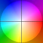
Figure 3: Color Wheel.

The used parameters are reported for each experiment separately, except for the discretization parameters $\Delta_{x},\Delta_{y},\Delta_{t}$, defined in Section 5. In this work we consider the following four dynamic image sequences:

• The first experiment is performed with the video sequence from [19] (available at http://of-eval.sourceforge.net/) which consists of forty-six frames showing a rotating sphere with some overlaid patterns. The analytical results from Appendix A in 1D suggest that the intensity of the $\vec{u}^{(2)}$ component increases monotonically with increasing rotational frequency over time. We verify this hypothesis numerically, now in higher dimensions. We simulate in particular two, four and eight times the original motion frequency;: In order to do so, we duplicate the sequence periodically, however consider it to be recorded in the same time interval $(0,1)$. The flow visualized in Figure 4 is the one between the 16th and the 17th frame of every sequence. We study the behavior of the sphere at different motion frequencies with the same parameter setting $\alpha^{(1)}=1$, $\alpha^{(2)}=\frac{1}{4}$. The numerical results confirm the $1D$ observation that for high rotational movement $\vec{u}^{(2)}$ is dominant (cf. Figures 4) and $\vec{u}^{(1)}$ is always $20\%$ of $\vec{u}^{(2)}$; in particular $\vec{u}^{(1)}$ and $\vec{u}^{(2)}$ cannot be completely separated.

  

  

  

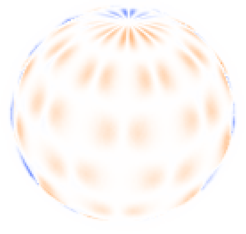
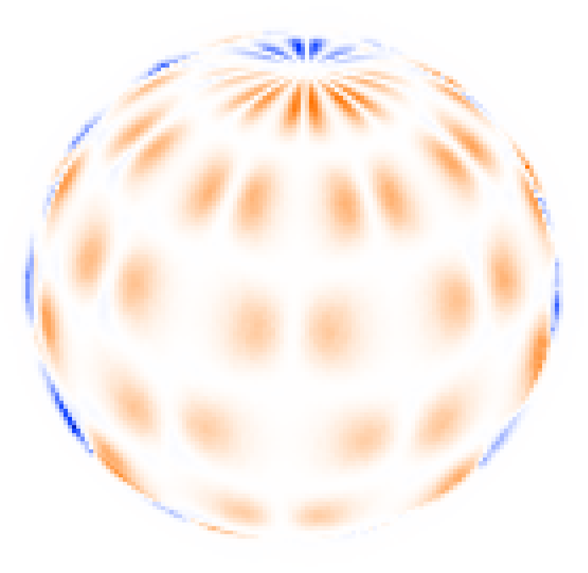
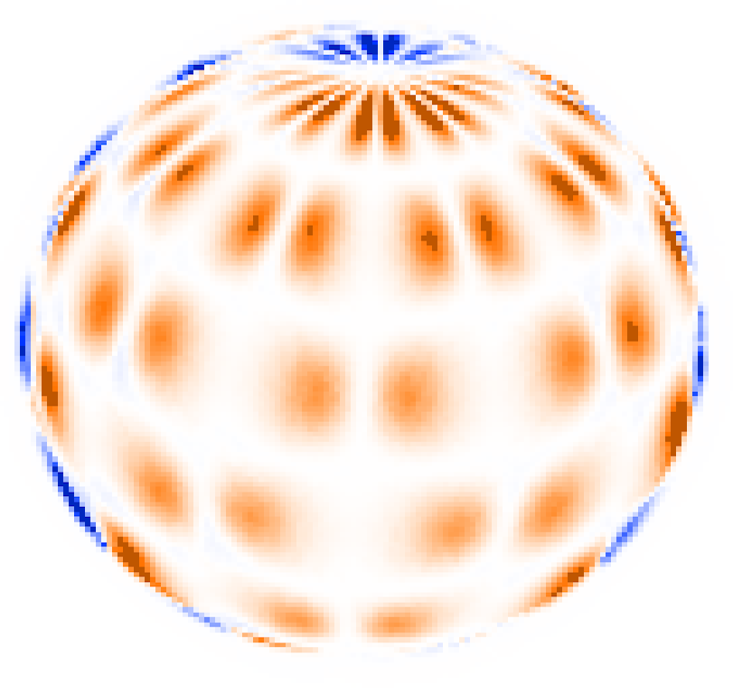
  Figure 4: $\vec{u}^{(2)}$ at different frequencies of rotations: $2$, $4$ and $8\times$ faster than the original motion frequency. $\alpha^{(1)}=1$, $\alpha^{(2)}=\frac{1}{4}$. The intensity of $\vec{u}^{(2)}$ increases when the frequency of rotation is increased.

• The second experiment concerns the decomposition of the motion in a dynamic image sequence showing a projection of a cube moving over an oscillating background. The movie consists of sixty frames and can be viewed on the web-page http://www.csc.univie.ac.at/index.php?page=visualattention.The background is oscillating in diagonal direction, from the bottom left to the top right, with a periodicity of four frames. In each frame the oscillation has a rate of $5\%$ of the frame size. The flow visualized in Figure 5 is the one between the 20th and the 21st frame of the sequence.

  Applying the proposed method with a parameter setting $\alpha^{(1)}=10^{3}$, $\alpha^{(2)}=10^{3}$, $\Delta_{\tau}=10^{-5}$, and precision tolerance $tol=0.001$, we notice that the background movement appears almost solely in $\vec{u}^{(2)}$ and the global movement of the cube appears in $\vec{u}^{(1)}$. In Figure 5 we represent only flow vectors with magnitude larger than $0.05$ and omit in $\vec{u}^{(2)}$ the part in common with $\vec{u}^{(1)}$ for better visibility.

  

  

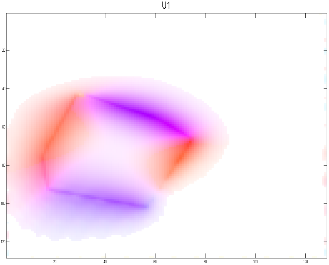
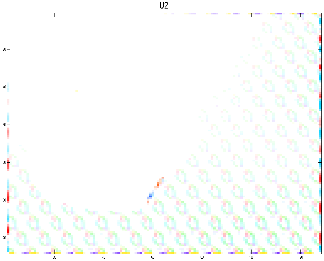
  Figure 5: The dynamic sequence consists of the smooth (translation like) motion of a cube and an oscillating background. The oscillation has a periodicity of four frames and takes place along the diagonal direction from the bottom left to the top right, moving at a rate of 5% of the frame size in each frame. The proposed model decomposes the motion, obtaining the global movement of the cube in $\vec{u}^{(1)}$ (left) and the background movement exclusively in $\vec{u}^{(2)}$ (right).

• In the third experiment the original movie consists of thirty-two frames and can be viewed together with the decomposition result on the web-page http://www.csc.univie.ac.at/index.php?page=visualattention. The flow is decomposed into two components. The first part shows the movement of a Ferris wheel and people walking. The second part shows blinking lights and the reflection of the wheel. The flow visualized in Figure 6 is the one between the 4th and the 5th frame of the sequence with a parameter setting $\alpha^{(1)}=1$, $\alpha^{(2)}=\frac{1}{4}$. In order to improve the visibility we represent only flow vectors with magnitude larger than $0.18$ and we omit for $\vec{u}^{(2)}$ the part in common with $\vec{u}^{(1)}$.

  

  

  

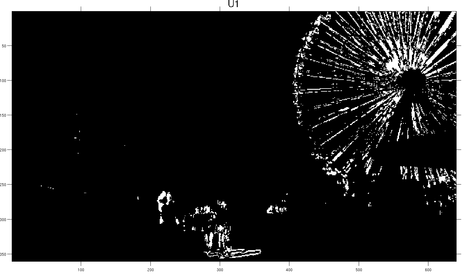
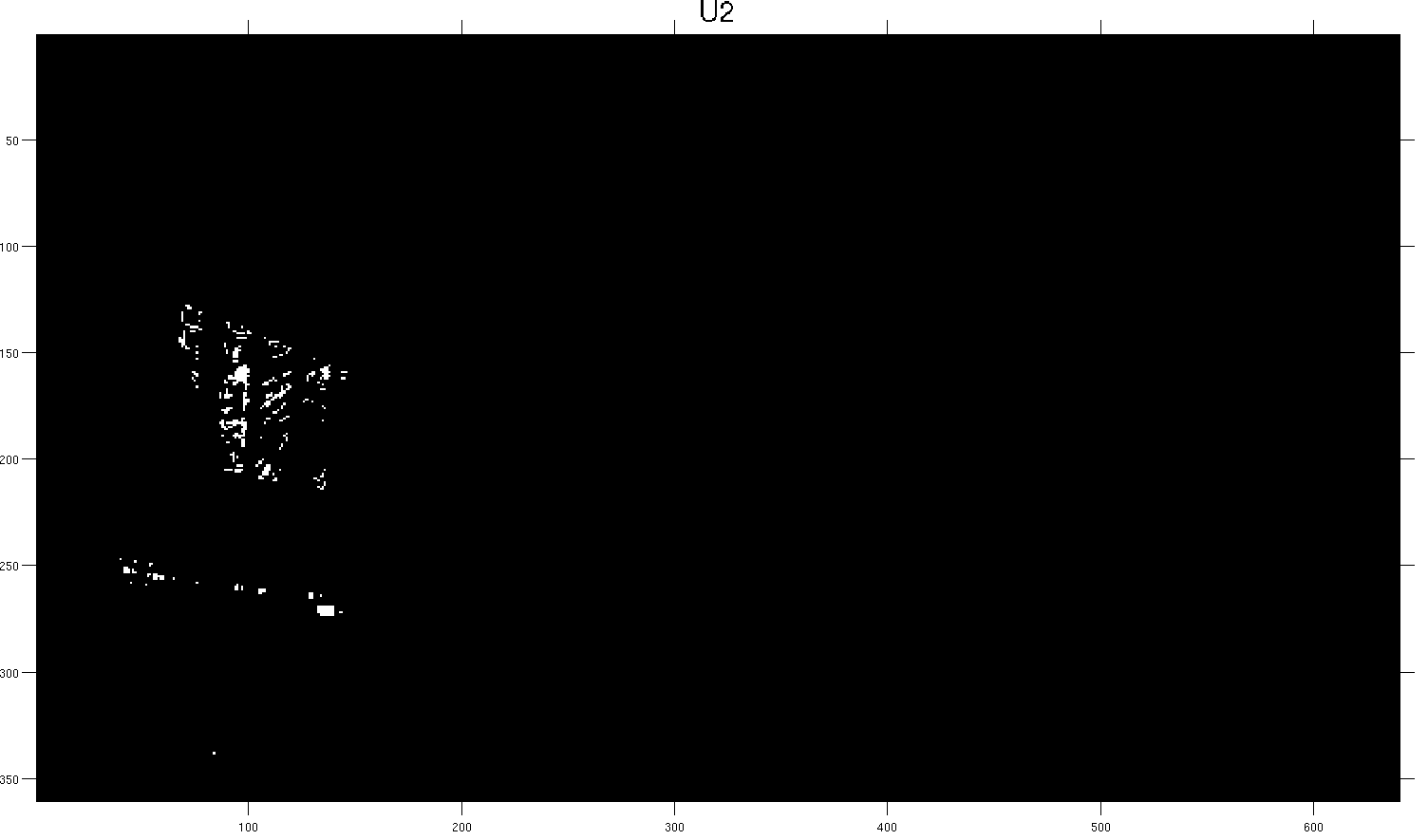
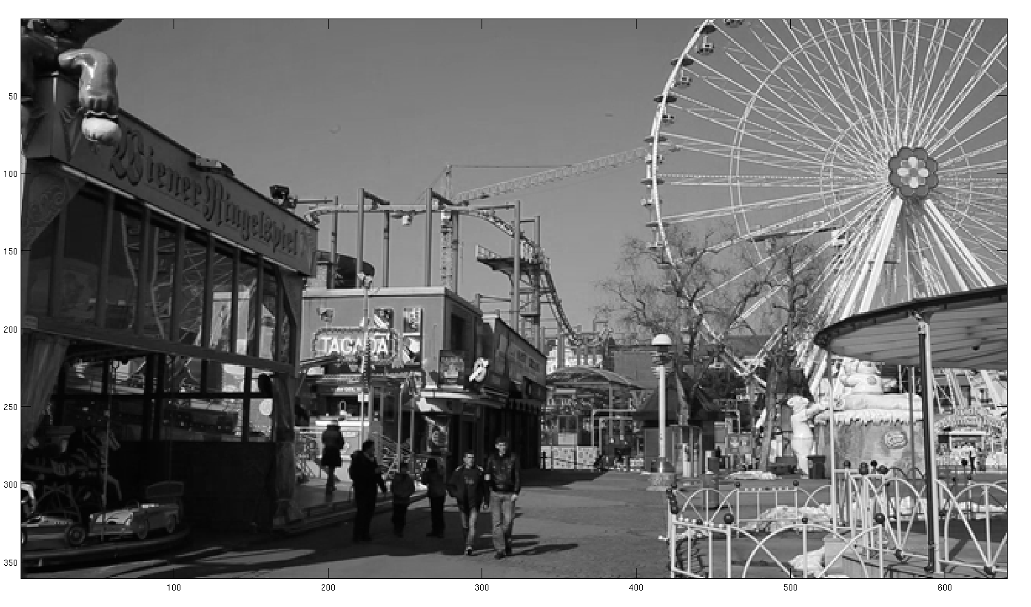
  Figure 6: $\vec{u}^{(1)}$: Movement of a Ferris wheel and people walking in the foreground (top left). $\vec{u}^{(2)}$ consists of blinking lights and the reflections of the wheel (top right). The third image (bottom) is a reference frame.

• The fourth example is flickering. In a standard flickering experiment, the difference in human attention is investigated by inclusion of blank images in a repetitive image sequence. Although, in general, these blank images are not deliberately recognized, they change the awareness of the test persons. J. K. O’Regan [22] states that “Change blindness is a phenomenon in which a very large change in a picture will not be seen by a viewer, if the change is accompanied by a visual disturbance that prevents attention from going to the change location”. They test data from http://nivea.psycho.univ-paris5.fr, was used for our simulations. The proposed optical flow decomposition is able to detect regions, which also humans can recognize, but standard optical flow algorithms fail to: To show this, the input sequence is composed by four frames consisting of Frame $1$, a blank image, Frame $2$ and again an identical blank image (see Figure 8 (top)). This sequence is then aligned periodically to a movie. We interpret the movie as a linear interpolation between the frames. We test and compare Horn-Schunck, Weickert-Schnörr and the proposed algorithm.

  

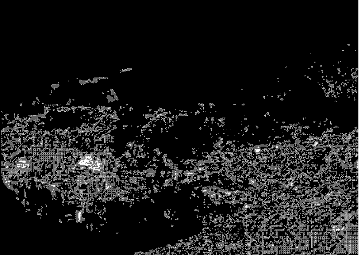
  Figure 7: Result with Horn-Schunck.

  We set the smoothness parameter $\alpha^{(1)}$ to a value of one for all the methods. Moreover, for our approach we set $\alpha^{(2)}=1$. For Horn-Schunck we visualize the flow field in Figure 7. This flow is the one between the blank frame and the slightly changed frame, which exceeds a threshold of $3.9$. The results obtained by applying Weickert-Schnörr and the $\vec{u}^{(1)}$ field of our approach, respectively, are small in magnitude. Therefore, we do not visualize them. This behavior is coherent with the motivation of the Weickert-Schnörr method to produce an optical flow that is less sensitive to variations over space and time. Finally, we visualize in Figure 8 (down right) the $\vec{u}^{(2)}$ flow field for the proposed approach. For the visualization we omit all vectors with magnitude lower than $0.18$. In order to make transparent the result, we show in Figure 8 (down left) the difference between the two frames of the sequence containing information (see Figure 8 (top)).

  

  

  

  

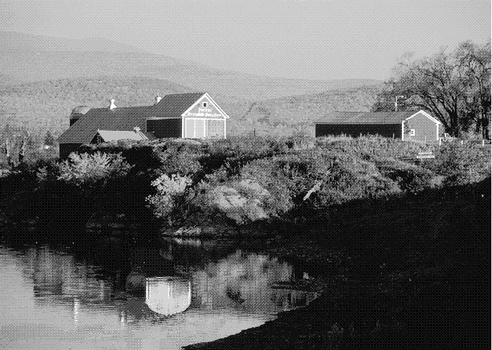
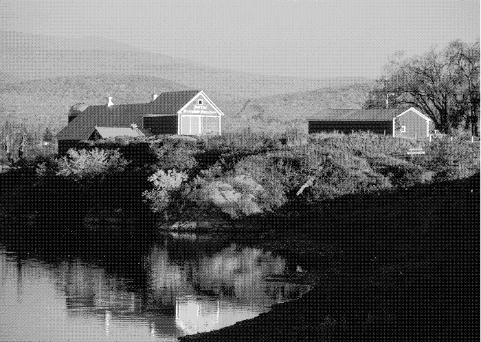
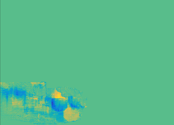
  Figure 8: The two frames of the flickering sequence containing information (top), the difference between these two frames (down left), and the $\vec{u}^{(2)}$ flow field resulting from the proposed approach (down right). As predicted in Section 3 and Appendix A the $\vec{u}^{(1)}$ component is negligible, instead $\vec{u}^{(2)}$ detects the change of intensity across the blank sheet.

  In this experiment, we notice that the $\vec{u}^{(1)}$ component is negligible, instead $\vec{u}^{(2)}$ detects the areas affected by change of intensities (see Figure 8 (down right)).

Additional Information

In the following, we show the capacity of our model to extract different information compared to standard optical flow algorithms. The current literature focuses on average angular and endpoint error [8] in order to compare optical flow algorithms. Our model extracts information, that is neglected by standard algorithms. Such difference can be shown through a quantitative comparison of models. For this purpose, we use well-known test sequences from the Middlebury database http://vision.middlebury.edu/flow/, and evaluate the residual of the optical flow constraint.

In order to understand how much information our method is capable to extract from an entire dynamic sequence, we calculate the residual squared over space and time: $\mathcal{E}(\vec{u}^{(1)},\vec{u}^{(2)})$ as in (10) and compare it with the squared residual over space and time of the Weickert-Schnörr method [28, 29]. We use the parameter settings $\alpha^{(1)}=100$ ($\alpha=\alpha^{(1)}$ in Weickert-Schnörr) and $\alpha^{(2)}=\frac{1}{4}$, tolerance $tol=0.01$, in order to have a good comparison of the two methods. Again the residual is smaller for the proposed method as shown in Table 3.

	Weickert-Schnörr	Proposed model
Hamburg Taxi	1374.9	1021
RubberWhale	4459.7	3046.8
Hydrangea	8533.3	7647.2
DogDance	9995.4	8217.6
Walking	8077.5	5944.3

Table 3: Comparison of squared residuals over space and time $\mathcal{E}$ between Weickert-Schnörr and the proposed method.

The smaller value of the residual are due to the fact that we are calculating a minimizer from a larger space of optical flow components. However, with this approach we cannot observe oversmoothing of the flow.

7 Conclusion

We present a new optical flow model for decomposing the flow in spatial and temporal components of different scales. A main ingredient of our work is a new variational formulation of the optical flow equation. Finally, applications (some of them from psychological experiments) are considered and analyzed analytically and computationally.

Appendix A Optical flow decomposition in 1D

In order to make transparent the features of our decomposition we study exemplary the 1D case again. From regularization theory (see e.g. [23]) we know that the minimizers $(u^{(1)}_{\vec{\alpha}}$, $u^{(2)}_{\vec{\alpha}})$, for $\vec{\alpha}=(\alpha^{(1)},\alpha^{(2)})\to 0$, are converging to a solution of the optical flow equation which minimizes

$$\mathcal{R}=\mathcal{R}^{(1)}+\alpha\mathcal{R}^{(2)}\text{ for }\alpha=\lim_{\vec{\alpha}\to 0}\frac{\alpha^{(2)}}{\alpha^{(1)}}>0\;.$$

Such a solution is called $\mathcal{R}$ minimizing solution. Note that by the 1D simplification the modules $u^{(i)}$, $i=1,2$, are real valued functions.

We calculate the decomposition for the optical flow equation (5), for the specific test data (6). The regularized solutions approximate the $\mathcal{R}$ minimizing solution, and thus these calculations can be viewed representative for the properties of the minimizer of the regularization method. For these particular kind of data the solution of the optical flow equation is given by :

$$u(x,t)=-\frac{\tilde{f}(x)}{\partial_{x}\tilde{f}(x)}\frac{\partial_{t}g(t)}{g(t)}=-\frac{\partial_{t}(\log g)(t)}{\partial_{x}(\log\tilde{f})(x)}\;.$$ (36)

Let us assume that $(\log g)(t)-(\log g)(0)$ can be expanded into a Fourier $\sin$-series:

$$(\log g)(t)-(\log g)(0)=\int_{0}^{t}\partial_{t}(\log g)(\tau)\,\mathrm{d}\tau=\sum_{n=1}^{\infty}\hat{g}_{n}\sin(n\pi t).$$ (37)

Moreover, we assume that $1/\partial_{x}(\log\tilde{f})(x)$ can be expanded in a $\cos$-series:

$$\frac{1}{\partial_{x}(\log\tilde{f})(x)}=\sum_{m=0}^{\infty}f_{m}\cos(m\pi x).$$ (38)

Then

$$-\frac{(\log g)(t)-(\log g)(0)}{\partial_{x}(\log\tilde{f})(x)}=\widehat{u}(x,t)=\widehat{u}^{(1)}(x,t)+\widehat{u}^{(2)}(x,t).$$ (39)

Inserting this identity in the regularization functional $\mathcal{R}(u^{(1)},u^{(2)})=\int(\partial_{x}u^{(1)})^{2}+(\partial_{t}u^{(1)})^{2}+\alpha\left(\widehat{u}^{(2)}\right)^{2}\mathrm{d}x\mathrm{d}t\,,$ we remove the $u^{(2)}$ dependence, and we get

$$\mathcal{R}(\widehat{u}^{(1)}):=\int_{(0,1)\times(0,1)}\!\!\!\!\!\!\!(\partial_{xt}\widehat{u}^{(1)})^{2}+(\partial_{tt}\widehat{u}^{(1)})^{2}+\alpha\left(\frac{(\log g)(t)-(\log g)(0)}{\partial_{x}(\log\tilde{f})(x)}+\widehat{u}^{(1)}\right)^{2}\mathrm{d}x\mathrm{d}t,$$

where we enforce the following boundary conditions on $\widehat{u}^{(1)}$: From the definition of $\widehat{u}^{(1)}$ it follows that $\widehat{u}^{(1)}(x,0)=0.$ Secondly, we enforce $\widehat{u}^{(1)}(x,1)=0$. In fact, the assumption is reasonable, because when the series $\sum_{n=0}^{\infty}\hat{g}_{n}$ is absolutely convergent, $(\log g)(t)-(\log g)(0)=0$ (cf. (37)), which implies that $\widehat{u}^{(1)}(x,1)+\widehat{u}^{(2)}(x,1)=0$ (cf. (37)).

By substituting the relation between $\widehat{u}^{(2)}$ and $\widehat{u}^{(1)}$ we reduce the constraint optimization problem to an unconstrained optimization problem for $\widehat{u}^{(1)}$, and the minimizer solves the partial differential equation

$$\partial_{ttxx}\widehat{u}^{(1)}+\partial_{tttt}\widehat{u}^{(1)}+\alpha\left(\frac{(\log g)(t)-(\log g)(0)}{\partial_{x}(\log\tilde{f})(x)}+\widehat{u}^{(1)}\right)=0\text{ in }(0,1)\times(0,1),$$

together with the boundary conditions:

$$\partial_{tt}\widehat{u}^{(1)}=\widehat{u}^{(1)} =0\text{ on }(0,1)\times\left\{0,1\right\},$$ (40)

$$\partial_{x}\partial_{tt}\widehat{u}^{(1)} =0\text{ on }\left\{0,1\right\}\times(0,1).$$

The boundary conditions $\partial_{tt}\widehat{u}^{(1)}==0\text{ on }(0,1)\times\left\{0,1\right\},$ and $\partial_{x}\partial_{tt}\widehat{u}^{(1)}=0\text{ on }\left\{0,1\right\}\times(0,1)$ appear as natural boundary conditions, when weak solutions are considered.

Now, we substitute $\hat{w}:=\partial_{tt}\widehat{u}^{(1)},$ and we get the following system of equations

$$\partial_{xx}\hat{w}+\partial_{tt}\hat{w} =-\alpha\left(\frac{(\log g)(t)-(\log g)(0)}{\partial_{x}(\log\tilde{f})(x)}+\widehat{u}^{(1)}\right)\text{ in }(0,1)\times(0,1),$$ (41)

$$\hat{w} =0\text{ on }(0,1)\times\left\{0,1\right\},$$

$$\partial_{x}\hat{w} =0\text{ on }\left\{0,1\right\}\times(0,1).$$

and

$$\widehat{u}^{(1)}(x,t) =\int_{0}^{t}\int_{0}^{\tau}\hat{w}(x,\hat{\tau})\mathrm{d}\hat{\tau}\mathrm{d}\tau-t\int_{0}^{1}\int_{0}^{\tau}\hat{w}(x,\hat{\tau})\mathrm{d}\hat{\tau}\mathrm{d}\tau.$$

$\hat{w}$ can be expanded as follows:

$$\hat{w}(x,t)=\sum_{m,n=0}^{\infty}\hat{w}_{mn}\cos(m\pi x)\sin(n\pi t),$$

and we expand $\widehat{u}^{(1)}$ in an analogous manner:

$$\widehat{u}^{(1)}(x,t)=\sum_{m,n=0}^{\infty}\widehat{u}^{(1)}_{mn}\cos(m\pi x)\sin(n\pi t)\;,$$

such that

$$\hat{w}_{mn}=-n^{2}\pi^{2}\widehat{u}^{(1)}_{mn},\quad\forall\,m,n\in\mathbbm{N}_{0}.$$ (42)

Thus it follows from (41) that

$$\hat{w}_{mn}(m^{2}+n^{2})\pi^{2}=\alpha\left(\widehat{u}^{(1)}_{mn}+f_{m}\hat{g}_{n}\right),\quad\forall\,m,n\in\mathbbm{N}_{0}.$$ (43)

(42) and (43) imply that

$$\widehat{u}^{(1)}_{mn}=-\frac{\alpha}{\alpha+\pi^{4}(m^{2}+n^{2})n^{2}}f_{m}\hat{g}_{n},\quad\forall\,m,n\in\mathbbm{N}_{0}.$$ (44)

Now, consider a specific test example $g(t)=\exp\left\{\frac{\sin(n_{0}\pi t)}{n_{0}\pi}\right\}$ for some $n_{0}\in\mathbbm{N}$. Then, from (36) it follows that $u(x,t)=-\frac{\cos(n_{0}\pi t)}{\partial_{x}(\log\tilde{f})(x)},$ and correspondingly we have

$$(\log g)(t)-(\log g)(0)=\frac{\sin(n_{0}\pi t)}{n_{0}\pi}=\sum_{n=1}^{\infty}\frac{\delta_{nn_{0}}}{n_{0}\pi}\sin(n\pi t).$$

In this case it follows from (44) that

$$\widehat{u}^{(1)}_{mn}=-\frac{\alpha}{\alpha+\pi^{4}(m^{2}+n_{0}^{2})n_{0}^{2}}\frac{\delta_{nn_{0}}}{n_{0}\pi}f_{m}.$$

In the case of flickering data $f$, $u^{(2)}$ is pronounced (if $n_{0}$ is large $\widehat{u}^{(1)}_{mn}\approx 0)$ while in the quasi-static case $u^{(1)}$ is dominant. Moreover, we also see that spatial components belonging to Fourier-$\cos$ coefficients with large $m$ are more pronounced in the $u^{(2)}$ component, and the spatial and temporal coefficients always appear in both components. In particular this means that a threshold has to be set, to assign them to the first or second module.

References

- [1] Abhau J, Belhachmi Z, Scherzer O On a decomposition model for optical flow. In: Energy Minimization Methods in Computer Vision and Pattern Recognition, Lecture Notes in Computer Science, vol 5681, Springer-Verlag, Berlin, Heidelberg, 2009, pp 126–139, DOI 10.1007/978-3-642-03641-5˙10, URL http://dx.doi.org/10.1007/978-3-642-03641-5_10
- [2] Andreev R, Scherzer O and Zulehner W Simultaneous optical flow and source estimation: space-time discretization and preconditioning. Applied Numerical Mathematics 96, 2015, 72-81
- [3] Aubert G, Aujol JF Modeling very oscillating signals. Application to image processing. Appl Math Optim 51(2), 2005, 163–182
- [4] Aujol JF, Chambolle A Dual norms and image decomposition models. Int J Comput Vision 63(1), 2005, 85–104
- [5] Aujol JF, Kang S Color image decomposition and restoration. J Vis Commun Image Represent 17(4), 2006, 916–928DOI 10.1016/j.jvcir.2005.02.001, URL http://www.sciencedirect.com/science/article/B6WMK-4FTWJGT-1/2/ffd97bf7a31e0b9cfdc8af0895369e84
- [6] Aujol JF, Aubert G, Blanc-Féraud L, Chambolle A Image decomposition into a bounded variation component and an oscillating component. J Math Imaging Vision 22(1), 2005, 71–88
- [7] Aujol JF, Gilboa G, Chan T, Osher S Structure-texture image decomposition—modeling, algorithms, and parameter selection. Int J Comput Vision 67(1), 2006, 111–136
- [8] Baker S, Scharstein D, Lewis JP, Roth S, Black MJ, Szeliski R A database and evaluation methodology for optical flow. Int J Comput Vision 92(1), 2011, 1–31, DOI 10.1007/s11263-010-0390-2, URL http://www.springerlink.com/index/10.1007/s11263-010-0390-2
- [9] Bauer M, Bruveris M,Michor W.P. Overview of the geometries of shape spaces and diffeomorphism groups. J Math Imaging Vision 50(1-2), 2014, 60–97, DOI 10.1007/s10851-013-0490-z, URL http://dx.doi.org/10.1007/s10851-013-0490-z
- [10] Berkels B, Effland A and Rumpf M Time discrete geodesic paths in the space of images. ArXiv 2015 URL http://arxiv.org/abs/1503.02001
- [11] Borzi A, Ito K, and Kunisch K Optimal control formulation for determining optical flow. SIAM J Sci Comput 24(3), 2002, 818–847
- [12] Bruhn A Variational optic flow computation: Accurate modeling and efficient numerics. PhD thesis 2006, Saarland University, Germany
- [13] Duval V, Aujol JF, Vese L Mathematical modeling of textures: Application to color image decomposition with a projected gradient algorithm. J Math Imaging Vision 37, 2010, 232–248
- [14] Hanke M, Scherzer O Inverse problems light: numerical differentiation. Amer. Math. Monthly 108(6), 2001, 512–521 DOI 10.2307/2695705, URL http://dx.doi.org/10.2307/2695705
- [15] Horn BKP, Schunck BG Determining optical flow. Artificial Intelligence 17, 1981, 185–203
- [16] Jain A, Younes L A kernel class allowing for fast computations in shape spaces induced by diffeomorphisms. J Comput and Applied Math 245, 2013, 162–181 DOI 10.1016/j.cam.2012.10.019, URL http://dx.doi.org/10.1016/j.cam.2012.10.019
- [17] Kirisits C, Lang L, Scherzer O Decomposition of optical flow on the sphere. GEM-Int J on Geomathematics 5(1), 2014, 117–141, DOI 10.1007/s13137-013-0055-8, URL http://dx.doi.org/10.1007/s13137-013-0055-8
- [18] Kohlberger T, Memin E, Schnörr C Variational dense motion estimation using the helmholtz decomposition. In: Griffin LD, Lillholm M (eds) Scale Space Methods in Computer Vision, Lecture Notes in Computer Science, vol 2695, Springer, Berlin, 2003, 432–448, DOI 10.1007/3-540-44935-3˙30, URL http://dx.doi.org/10.1007/3-540-44935-3_30
- [19] McCane B, Novins K, Crannitch D, Galvin B On benchmarking optical flow. Comput Vision Image Understanding 84, 2001, 126–143
- [20] Meyer Y Oscillating patterns in image processing and nonlinear evolution equations, University Lecture Series, vol 22, 2001. American Mathematical Society, Providence, RI, the fifteenth Dean Jacqueline B. Lewis memorial lectures
- [21] Miller M I, Younes L Group actions, homeomorphisms, and matching: A general framework Int J Comput Vision 41(1/2), 2001, 61–84,
- [22] O’Regan JK Change blindness. E Cognitive science, 2007
- [23] Scherzer O, Grasmair M, Grossauer H, Haltmeier M, Lenzen F Variational methods in imaging, Applied Mathematical Sciences, vol 167, 2009. Springer, New York, DOI 10.1007/978-0-387-69277-7, URL http://dx.doi.org/10.1007/978-0-387-69277-7
- [24] Vese L, Osher S Modeling textures with total variation minimization and oscillating patterns in image processing. J Sci Comput 19(1–3), 2003, 553–572, special issue in honor of the sixtieth birthday of Stanley Osher
- [25] Vese L, Osher S Image denoising and decomposition with total variation minimization and oscillatory functions. J Math Imaging Vision 20, 2004, 7–18
- [26] Wang CM, Fan KC, Wang CT Estimating Optical Flow by Integrating Multi-Frame Information. Journal of Information Science and Engineering 24, 2008, 1719–1731
- [27] Weickert J, Bruhn A, Brox T, Papenberg N A Survey on Variational Optic Flow Methods for Small Displacements. Mathematical Models for Registration and Applications to Medical Imaging, Springer Berlin Heidelberg 10, 2006, 103–136 URL http://dx.doi.org/10.1007/978-3-540-34767-5_5
- [28] Weickert J, Schnörr C A theoretical framework for convex regularizers in PDE-based computation of image motion. Int J Comput Vision 45(3), 2001a, 245–264
- [29] Weickert J, Schnörr C Variational optic flow computation with a spatio-temporal smoothness constraint. J Math Imaging Vision 14, 2001b, 245–255
- [30] Yuan J, Schörr C, Steidl G Simultaneous higher-order optical flow estimation and decomposition. SIAM J Sci and Stat Comput 29(6), 2007, 2283–2304 (electronic), DOI 10.1137/060660709, URL http://dx.doi.org/10.1137/060660709
- [31] Yuan J, Steidl G, Schnörr C Convex Hodge decomposition of image flows. In: Pattern recognition, Lecture Notes in Comput. Sci., vol 5096, Springer, Berlin, 2008, 416–425, DOI 10.1007/978-3-540-69321-5˙42, URL http://dx.doi.org/10.1007/978-3-540-69321-5_42
- [32] Yuan J, Schnörr C, Steidl G Convex Hodge decomposition and regularization of image flows. J Math Imaging Vision 33(2), 2009, 169–177, DOI 10.1007/s10851-008-0122-1, URL http://dx.doi.org/10.1007/s10851-008-0122-1
- [33] Lee, Jungpyo and Wright, John C A versatile parallel block-tridiagonal solver for spectral codes. MIT Plasma Science & Fusion Center 2010