Subset Simulation Method for Rare Event Estimation: An Introduction

Abstract

This paper provides a detailed introductory description of Subset Simulation, an advanced stochastic simulation method for estimation of small probabilities of rare failure events. A simple and intuitive derivation of the method is given along with the discussion on its implementation. The method is illustrated with several easy-to-understand examples. For demonstration purposes, the MATLAB code for the considered examples is provided. The reader is assumed to be familiar only with elementary probability theory and statistics.

I Introduction

Subset Simulation (SS) is an efficient and elegant method for simulating rare events and estimating the corresponding small tail probabilities. The method was originally developed by Siu-Kui Au and James Beck in the already classical paper AuBeck for estimation of structural reliability of complex civil engineering systems such as tall buildings and bridges at risk from earthquakes. The method turned out to be so powerful and general that over the last decade, SS has been successfully applied to reliability problems in geotechnical, aerospace, fire, and nuclear engineering. Moreover, the idea of SS proved to be useful not only in reliability analysis but also in other problems associated with general engineering systems, such as sensitivity analysis, design optimization, and uncertainty quantification. As of October 2013, according to the Web of Knowledge database, the original SS paper AuBeck received more than 250 citations that indicates the high impact of the Subset Simulation method on the engineering research community.

Subset Simulation is essentially based on two different ideas: conceptual and technical. The conceptual idea is to decompose the rare event $F$ into a sequence of progressively “less-rare” nested events,

$$F=F_{m}\subset F_{m-1}\subset\ldots\subset F_{1},$$ (1)

where $F_{1}$ is a relatively frequent event. For example, suppose that $F$ represents the event of getting exactly $m$ heads when flipping a fair coin $m$ times. If $m$ is large, then $F$ is a rare event. To decompose $F$ into a sequence (1), let us define $F_{k}$ to be the event of getting exactly $k$ heads in the first $k$ flips, where $k=1,\ldots,m$. The smaller $k$, the less rare the corresponding event $F_{k}$; and $F_{1}$ — getting heads in the first flip — is relatively frequent.

Given a sequence of subsets (1), the small probability $\mathbb{P}(F)$ of the rare event $F$ can then be represented as a product of larger probabilities as follows:

$$\begin{split}\mathbb{P}(F)&=\mathbb{P}(F_{m})\\ &=\mathbb{P}(F_{1})\frac{\mathbb{P}(F_{2})}{\mathbb{P}(F_{1})}\frac{\mathbb{P}(F_{3})}{\mathbb{P}(F_{2})}\ldots\frac{\mathbb{P}(F_{m-1})}{\mathbb{P}(F_{m-2})}\frac{\mathbb{P}(F_{m})}{\mathbb{P}(F_{m-1})}\\ &=\mathbb{P}(F_{1})\cdot\mathbb{P}(F_{2}|F_{1})\cdot\ldots\cdot\mathbb{P}(F_{m}|F_{m-1}),\end{split}$$ (2)

where $\mathbb{P}(F_{k}|F_{k-1})=\mathbb{P}(F_{k})/\mathbb{P}(F_{k-1})$ denotes the conditional probability of event $F_{k}$ given the occurrence of event $F_{k-1}$, for $k=2,\ldots,m$. In the coin example, $\mathbb{P}(F_{1})=1/2$, all conditional probabilities $\mathbb{P}(F_{k}|F_{k-1})=1/2$, and the probability of the rare event $\mathbb{P}(F)=1/2^{m}$.

Unlike the coin example, in real applications, it is often not obvious how to decompose the rare event into a sequence (1) and how to compute all conditional probabilities in (2). In Subset Simulation, the “sequencing” of the rare event is done adaptively as the algorithm proceeds. This is achieved by employing Markov chain Monte Carlo, an advanced simulation technique, which constitutes the second – technical – idea behind SS. Finally, all conditional probabilities are automatically obtained as a by-product of the adaptive sequencing.

The main goals of this paper are: (a) to provide a detailed exposition of Subset Simulation at an introductory level; (b) to give a simple derivation of the method and discuss its implementation; and (c) to illustrate SS with intuitive examples. Although the scope of SS is much wider, in this paper the method is described in the context of engineering reliability estimation, the problem SS was originally developed for in AuBeck .

The rest of the paper is organized as follows. Section II describes the engineering reliability problem and explains why this problem is computationally challenging. Section III discusses how the direct Monte Carlo method can be used for engineering reliability estimation and why it is often inefficient. In Section IV, a necessary preprocessing step which is often used by many reliability methods is briefly discussed. Section V is the core of the paper, where the SS method is explained. Illustrative examples are considered in Section  VI. For demonstration purposes, the MATLAB code for the considered examples is provided in Section VII. Section VIII concludes the paper with a brief summary.

II Engineering Reliability Problem

One of the most important and computationally challenging problems in reliability engineering is to estimate the probability of failure for a system, that is, the probability of unacceptable system performance. The behavior of the system can be described by a response variable $y$, which may represent, for example, the roof displacement or the largest interstory drift. The response variable depends on input variables $x=(x_{1},\ldots,x_{d})$, also called basic variables, which may represent geometry, material properties, and loads,

$$y=g(x_{1},\ldots,x_{d}),$$ (3)

where $g(x)$ is called the performance function. The performance of the system is measured by comparison of the response $y$ with a specified critical value $y^{*}$: if $y\leq y^{*}$, then the system is safe; if $y>y^{*}$, then the system has failed. This failure criterion allows to define the failure domain $F$ in the input $x$-space as follows:

$$F=\{x~{}:~{}g(x)>y^{*}\}.$$ (4)

In other words, the failure domain is a set of values of input variables that lead to unacceptance system performance, namely, to the exceedance of some prescribed critical threshold $y^{*}$, which may represent the maximum permissible roof displacement, maximum permissible interstory drift, etc.

Engineering systems are complex systems, where complexity, in particular, means that the information about the system (its geometric and material properties) and its environment (loads) is never complete. Therefore, there are always uncertainties in the values of input variables $x$. To account for these uncertainties, the input variables are modeled as random variables whose marginal distributions are usually obtained from test data, expert opinion, or from literature. Let $\pi(x)$ denote the join probability density function (PDF) for $x$. The randomness in the input variables is propagated through (3) into the response variable $y$, which makes the failure event $\{x\in F\}=\{y>y^{*}\}$ also random. The engineering reliability problem is then to compute the probability of failure $p_{F}$, given by the following expression:

$$p_{F}=\mathbb{P}(x\in F)=\int_{F}\pi(x)dx.$$ (5)

The behavior of complex systems, such as tall buildings and bridges, is represented by a complex model (3). In this context, complexity means that the performance function $g(x)$, which defines the integration region $F$ in (5), is not explicitly known. The evaluation of $g(x)$ for any $x$ is often time-consuming and usually done by the finite element method (FEM), one of the most important numerical tools for computation of the response of engineering systems. Thus, it is usually impossible to evaluate the integral in (5) analytically because the integration region, the failure domain $F$, is not known explicitly.

Moreover, traditional numerical integration is also generally not applicable. In this approach, the $d$-dimensional input $x$-space is partitioned into a union of disjoint hypercubes, $\square_{1},\ldots,\square_{N}$. For each hypercube $\square_{i}$, a “representative” point $x^{(i)}$ is chosen inside that hypercube, $x^{(i)}\in\square_{i}$. The integral in (5) is then approximated by the following sum:

$$p_{F}\approx\sum_{x^{(i)}\in F}\pi(x^{(i)})\mathrm{vol}(\square_{i}),$$ (6)

where $\mathrm{vol}(\square_{i})$ denotes the volume of $\square_{i}$ and summation is taken over all failure points $x^{(i)}$. Since it is not known in advance whether a given point is a failure point or not (the failure domain $F$ is not known explicitly), to compute the sum in (6), the failure criterion (4) must be checked for all $x^{(i)}$. Therefore, the approximation (6) becomes

$$p_{F}\approx\sum_{i=1}^{N}I_{F}(x^{(i)})\pi(x^{(i)})\mathrm{vol}(\square_{i}),$$ (7)

where $I_{F}(x)$ stands for the indicator function, i.e.,

$$I_{F}(x)=\left\{\begin{array}[]{ll}1,&\hbox{if $x\in F$,}\\ 0,&\hbox{if $x\notin F$.}\end{array}\right.$$ (8)

If $n$ denotes the number of intervals each dimension of the input space is partitioned into, then the total number of terms in (7) is $N=n^{d}$. Therefore, the computational effort of numerical integration grows exponentially with the number of dimensions $d$. In engineering reliability problems, the dimension of the input space is typically very large (e.g., when the stochastic load time history is discretized in time). For example, $d\sim 10^{3}$ is not unusual in the reliability literature. This makes numerical integration computationally infeasible.

Over the past few decades, many different methods for solving the engineering reliability problem (5) have been developed. In general, the proposed reliability methods can be classified into three categories, namely:

1. Analytic methods are based on the Taylor-series expansion of the performance function, e.g. the First-Order Reliability Method (FORM) and the Second-Order Reliability Method (SORM) Ditlevsen ; Madsen ; Melchers .

2. Surrogate methods are based on a functional surrogate of the performance function, e.g. the Response Surface Method (RSM) Faravelli ; Schueller ; Bucher , Neural Networks Papadrakakis , Support Vector Machines Hurtado , and other methods Hurtado_book .

3. Monte Carlo simulation methods, among which are Importance Sampling Engelund , Importance Sampling using Elementary Events AuBeck2 , Radial-based Importance Sampling Grooteman , Adaptive Linked Importance Sampling ALIS , Directional Simulation Ditlevsen , Line Sampling LineSampling , Auxiliary Domain Method ADM , Horseracing Simulation Zuev , and Subset Simulation AuBeck .

Subset Simulation is thus a reliability method which is based on (advanced) Monte Carlo simulation.

III The Direct Monte Carlo Method

The Monte Carlo method, referred in this paper as Direct Monte Carlo (DMC), is a statistical sampling technique that have been originally developed by Stan Ulam, John von Neumann, Nick Metropolis (who actually suggested the name “Monte Carlo” Metropolis ), and their collaborators for solving the problem of neutron diffusion and other problems in mathematical physics MonteCarlo . From a mathematical point of view, DMC allows to estimate the expected value of a quantity of interest. More specifically, suppose the goal is to evaluate $\mathbb{E}_{\pi}[h(x)]$, that is an expectation of a function $h:\mathcal{X}\rightarrow\mathbb{R}$ with respect to the PDF $\pi(x)$,

$$\mathbb{E}_{\pi}[h(x)]=\int_{\mathcal{X}}h(x)\pi(x)dx.$$ (9)

The idea behind DMC is a straightforward application of the law of large numbers that states that if $x^{(1)},x^{(2)},\ldots$ are i.i.d. (independent and identically distributed) from the PDF $\pi(x)$, then the empirical average $\frac{1}{N}\sum_{i=1}^{N}h(x^{(i)})$ converges to the true value $\mathbb{E}_{\pi}[h(x)]$ as $N$ goes to $+\infty$. Therefore, if the number of samples $N$ is large enough, then $\mathbb{E}_{\pi}[h(x)]$ can be accurately estimated by the corresponding empirical average:

$$\mathbb{E}_{\pi}[h(x)]\approx\frac{1}{N}\sum_{i=1}^{N}h(x^{(i)}).$$ (10)

The relevance of DMC to the reliability problem (5) follows from a simple observation that the failure probability $p_{F}$ can be written as an expectation of the indicator function (8), namely,

$$p_{F}=\int_{F}\pi(x)dx=\int_{\mathcal{X}}I_{F}(x)\pi(x)dx=\mathbb{E}_{\pi}[I_{F}(x)],$$ (11)

where $\mathcal{X}$ denotes the entire input $x$-space. Therefore, the failure probability can be estimated using the DMC method (10) as follows:

$$p_{F}\approx\hat{p}_{F}^{\mbox{\tiny{DMC}}}=\frac{1}{N}\sum_{i=1}^{N}I_{F}(x^{(i)}),$$ (12)

where $x^{(1)},\ldots x^{(N)}$ are i.i.d. samples from $\pi(x)$.

The DMC estimate of $p_{F}$ is thus just the ratio of the total number of failure samples $\sum_{i=1}^{N}I_{F}(x^{(i)})$, i.e., samples that produce system failure according to the system model, to the total number of samples, $N$. Note that $\hat{p}_{F}^{\mbox{\tiny{DMC}}}$ is an unbiased random estimate of the failure probability, that is, on average, $\hat{p}_{F}^{\mbox{\tiny{DMC}}}$ equals to $p_{F}$. Mathematically, this means that $\mathbb{E}[\hat{p}_{F}^{\mbox{\tiny{DMC}}}]=p_{F}$. Indeed, using the fact that $x^{(i)}\sim\pi(x)$ and (11),

$$\begin{split}\mathbb{E}[\hat{p}_{F}^{\mbox{\tiny{DMC}}}]&=\mathbb{E}\left[\frac{1}{N}\sum_{i=1}^{N}I_{F}(x^{(i)})\right]\\ &=\frac{1}{N}\sum_{i=1}^{N}\mathbb{E}[I_{F}(x^{(i)})]\\ &=\frac{1}{N}\sum_{i=1}^{N}\mathbb{E}_{\pi}[I_{F}(x)]=p_{F}.\end{split}$$ (13)

The main advantage of DMC over numerical integration is that its accuracy does not depend on the dimension $d$ of the input space. In reliability analysis, the standard measure of accuracy of an unbiased estimate $\hat{p}_{F}$ of the failure probability is its coefficient of variation (c.o.v.) $\delta(\hat{p}_{F})$, which is defined as the ratio of the standard deviation to the expected value of $\hat{p}_{F}$, i.e., $\delta(\hat{p}_{F})=\sqrt{\mathbb{V}[\hat{p}_{F}]}/\mathbb{E}[\hat{p}_{F}]$, where $\mathbb{V}$ denotes the variance. The smaller the c.o.v. $\delta(\hat{p}_{F})$, the more accurate the estimate $\hat{p}_{F}$ is. It is straightforward to calculate the variance of the DMC estimate:

$$\begin{split}\mathbb{V}[\hat{p}_{F}^{\mbox{\tiny{DMC}}}]&=\mathbb{V}\left[\frac{1}{N}\sum_{i=1}^{N}I_{F}(x^{(i)})\right]\\ &=\frac{1}{N^{2}}\sum_{i=1}^{N}\mathbb{V}[I_{F}(x^{(i)})]\\ &=\frac{1}{N^{2}}\sum_{i=1}^{N}\left(\mathbb{E}[I_{F}(x^{(i)})^{2}]-\mathbb{E}[I_{F}(x^{(i)})]^{2}\right)\\ &=\frac{1}{N^{2}}\sum_{i=1}^{N}\left(p_{F}-p_{F}^{2}\right)=\frac{p_{F}(1-p_{F})}{N}.\end{split}$$ (14)

Here, the identity $I_{F}(x)^{2}=I_{F}(x)$ was used. Using (13) and (14), the c.o.v. of the DMC estimate can be calculated:

$$\delta(\hat{p}_{F}^{\mbox{\tiny{DMC}}})=\frac{\sqrt{\mathbb{V}[\hat{p}_{F}^{\mbox{\tiny{DMC}}}]}}{\mathbb{E}[\hat{p}_{F}^{\mbox{\tiny{DMC}}}]}=\sqrt{\frac{1-p_{F}}{Np_{F}}}.$$ (15)

This result shows that $\delta(\hat{p}_{F}^{\mbox{\tiny{DMC}}})$ depends only on the failure probability $p_{F}$ and the total number of samples $N$, and does not depend on the dimension $d$ of the input space. Therefore, unlike numerical integration, the DMC method does not suffer from the “curse of dimensionality”, i.e. from an exponential increase in volume associated with adding extra dimensions, and is able to handle problems of high dimension.

Nevertheless, DMC has a serious drawback: it is inefficient in estimating small failure probabilities. For typical engineering reliability problems, the failure probability $p_{F}$ is very small, $p_{F}\ll 1$. In other words, the system is usually assumed to be designed properly, so that its failure is a rare event. In the reliability literature, $p_{F}\sim 10^{-2}-10^{-9}$ have been considered. If $p_{F}$ is very small, then it follows from (15) that

$$\delta(\hat{p}_{F}^{\mbox{\tiny{DMC}}})\approx\frac{1}{\sqrt{Np_{F}}}.$$ (16)

This means that the number of samples $N$ needed to achieve an acceptable level of accuracy is inverse proportional to $p_{F}$, and therefore very large, $N\propto 1/p_{F}\gg 1$. For example, if $p_{F}=10^{-4}$ and the c.o.v. of $10\%$ is desirable, then $N=10^{6}$ samples are required. Note, however, that each evaluation of $I_{F}(x^{(i)})$, $i=1,\ldots,N$, in (12) requires a system analysis to be performed to check whether the sample $x^{(i)}$ is a failure sample. As it has been already mentioned in Section II, the computation effort for the system analysis, i.e., computation of the performance function $g(x)$, is significant (usually involves the FEM method). As a result, the DMC method becomes excessively costly and practically inapplicable for reliability analysis. This deficiency of DMC has motivated research to develop more advanced simulation algorithms for efficient estimation of small failure probabilities in high dimensions.

Remark 1.

It is important to highlight, however, that even though DMC cannot be routinely used for reliability problems (too expensive), it is a very robust method, and it is often used as a check on other reliability methods.

IV Preprocessing: Transformation of Input Variables

Many reliability methods, including Subset Simulation, assume that the input variables $x$ are independent. This assumption, however, is not a limitation, since in simulation one always starts from independent variables to generate dependent “physical” variables. Furthermore, for convenience, it is often assumed that $x$ are i.i.d. Gaussian. If this is not the case, a “preprocessing” step that transforms $x$ to i.i.d. Gaussian variables $z$ must be undertaken. The transformation form $x$ to $z$ can be performed in several ways depending on the available information about the input variables. In the simplest case, when $x$ are independent Gaussians, $x_{k}\sim\mathcal{N}(\cdot|\mu_{k},\sigma_{k}^{2})$, where $\mu_{k}$ and $\sigma_{k}^{2}$ are respectively the mean and variance of $x_{k}$, the necessary transformation is standardization:

$$z_{k}=\frac{x_{k}-\mu_{k}}{\sigma_{k}}.$$ (17)

In other cases, more general techniques should be used, such as the Rosenblatt transformation Rosenblatt and the Nataf transformation Nataf . To avoid introduction of additional notation, hereinafter, it is assumed without loss of generality that the vector $x$ has been already transformed and it follows the standard multivariate Gaussian distribution,

$$\pi(x_{1},\ldots,x_{d})=\prod_{k=1}^{d}\phi(x_{k}),$$ (18)

where $\phi(\cdot)$ denotes the standard Gaussian PDF,

$$\phi(x)=\frac{1}{\sqrt{2\pi}}\,e^{-\frac{\scriptscriptstyle 1}{\scriptscriptstyle 2}x^{2}}.$$ (19)

V The Subset Simulation Method

Unlike Direct Monte Carlo, where all computational resources are directly spent on sampling the input space, $x^{(1)},\ldots,x^{(N)}\sim\pi(\cdot)$, and computing the values of the performance function $g(x^{(1)}),\ldots,g(x^{(N)})$, Subset Simulation first “probes” the input space $\mathcal{X}$ by generating a relatively small number of i.i.d samples $x^{(1)}_{0},\ldots,x^{(n)}_{0}\sim\pi(x)$, $n<N$, and computing the corresponding system responses $y_{0}^{(1)}=g(x_{0}^{(1)}),\ldots,y_{0}^{(n)}=g(x_{0}^{(n)})$. Here, the subscript 0 indicates the $0^{\mathrm{th}}$ stage of the algorithm. Since $F$ is a rare event and $n$ is relatively small, it is very likely that none of the samples $x^{(1)}_{0},\ldots,x^{(n)}_{0}$ belongs to $F$, that is $y_{0}^{(i)}<y^{*}$ for all $i=1,\ldots,n$. Nevertheless, these Monte Carlo samples contain some useful information about the failure domain that can be utilized. To keep the notation simple, assume that $y_{0}^{(1)},\ldots,y_{0}^{(n)}$ are arranged in the decreasing order, i.e. $y_{0}^{(1)}\geq\ldots\geq y_{0}^{(n)}$ (it is always possible to achieve this by renumbering $x^{(1)}_{0},\ldots,x^{(n)}_{0}$ if needed). Then, $x^{(1)}_{0}$ and $x^{(n)}_{0}$ are, respectively, the closest to failure and the safest samples among $x^{(1)}_{0},\ldots,x^{(n)}_{0}$, since $y_{0}^{(1)}$ and $y_{0}^{(n)}$ are the largest and the smallest responses. In general, the smaller $i$, the closer to failure the sample $x_{0}^{(i)}$ is. This is shown schematically in Fig. 1.

Let $p\in(0,1)$ be any number such that $np$ is integer. By analogy with (4), define the first intermediate failure domain $F_{1}$ as follows:

$$F_{1}=\{x~{}:~{}g(x)>y_{1}^{*}\},$$ (20)

where

$$y_{1}^{*}=\frac{y_{0}^{(np)}+y_{0}^{(np+1)}}{2}.$$ (21)

In other words, $F_{1}$ is the set of inputs that lead to the exceedance of the relaxed threshold $y^{*}_{1}<y^{*}$. Note that by construction, samples $x^{(1)}_{0},\ldots,x^{(np)}_{0}$ belong to $F_{1}$, while $x^{(np+1)}_{0},\ldots,x^{(n)}_{0}$ do not. As a consequence, the Direct Monte Carlo estimate for the probability of $F_{1}$ which is based on samples $x^{(1)}_{0},\ldots,x^{(n)}_{0}$ is automatically equal to $p$,

$$\mathbb{P}(F_{1})\approx\frac{1}{n}\sum_{i=1}^{n}I_{F_{1}}(x^{(i)}_{0})=p.$$ (22)

The value $p=0.1$ is often used in the literature, which makes $F_{1}$ a relatively frequent event. Fig. 2 illustrates the definition of $F_{1}$.

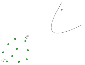
Figure 1: Monte Carlo samples $x^{(1)}_{0},\ldots,x^{(n)}_{0}$ and the failure domain $F$. $x^{(1)}_{0}$ and $x^{(n)}_{0}$ are, respectively, the closest to failure and the safest samples among $x^{(1)}_{0},\ldots,x^{(n)}_{0}$.

The first intermediate failure domain $F_{1}$ can be viewed as a (very rough) conservative approximation to the target failure domain $F$. Since $F\subset F_{1}$, the failure probability $p_{F}$ can be written as a product:

$$p_{F}=\mathbb{P}(F_{1})\mathbb{P}(F|F_{1}),$$ (23)

where $\mathbb{P}(F|F_{1})$ is the conditional probability of $F$ given $F_{1}$. Therefore, in view of (22), the problem of estimating $p_{F}$ is reduced to estimating the conditional probability $\mathbb{P}(F|F_{1})$.

In the next stage, instead of generating samples in the whole input space (like in DMC), the SS algorithm aims to populate $F_{1}$. Specifically, the goal is to generate samples $x^{(1)}_{1},\ldots,x^{(n)}_{1}$ from the conditional distribution

$$\pi(x|F_{1})=\frac{\pi(x)I_{F_{1}}(x)}{\mathbb{P}(F_{1})}=\frac{I_{F_{1}}(x)}{\mathbb{P}(F_{1})}\prod_{k=1}^{d}\phi(x_{k}).$$ (24)

First of all, note that samples $x^{(1)}_{0},\ldots,x^{(np)}_{0}$ not only belong to $F_{1}$, but are also distributed according to $\pi(\cdot|F_{1})$. To generate the remaining $(n-np)$ samples from $\pi(\cdot|F_{1})$, which, in general, is not a trivial task, Subset Simulation uses the so-called Modified Metropolis algorithm (MMA). MMA belongs to the class of Markov chain Monte Carlo (MCMC ) algorithms Liu ; Robert , which are techniques for sampling from complex probability distributions that cannot be sampled directly, at least not efficiently. MMA is based on the original Metropolis algorithm MA and specifically tailored for sampling from the conditional distributions of the form (24).

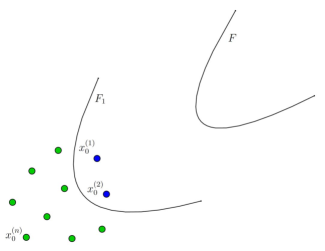
Figure 2: The first intermediate failure domain $F_{1}$. In this schematic illustration, $n=10$, $p=0.2$, so that there are exactly $np=2$ Monte Carlo samples in $F_{1}$, $x_{0}^{(1)},x_{0}^{(2)}\in F_{1}$.

V.1 Modified Metropolis algorithm

Let $x\sim\pi(\cdot|F_{1})$ be a sample from the conditional distribution $\pi(\cdot|F_{1})$. The Modified Metropolis algorithm generates another sample $\tilde{x}$ from $\pi(\cdot|F_{1})$ as follows:

1. Generate a “candidate” sample $\xi$:
   For each coordinate $k=1,\ldots,d,$

   1. Sample $\eta_{k}\sim q_{k}(\cdot|x_{k})$, where $q_{k}(\cdot|x_{k})$, called the proposal distribution, is a univariate PDF for $\eta_{k}$ centered at $x_{k}$ with the symmetry property $q_{k}(\eta_{k}|x_{k})=q_{k}(x_{k}|\eta_{k})$. For example, the proposal distribution can be a Gaussian PDF with mean $x_{k}$ and variance $\sigma^{2}_{k}$,

      $$q_{k}(\eta_{k}|x_{k})=\frac{1}{\sqrt{2\pi}\sigma_{k}}\,\exp\left(-\frac{(\eta_{k}-x_{k})^{2}}{2\sigma_{k}^{2}}\right),$$ (25)

      or it can be a uniform distribution over $[x_{k}-\alpha,x_{k}+\alpha]$, for some $\alpha\geq 0$.

   2. Compute the acceptance ratio

      $$r_{k}=\frac{\phi(\eta_{k})}{\phi(x_{k})}.$$ (26)

   3. Define the $k^{\mathrm{th}}$ coordinate of the candidate sample by accepting or rejecting $\eta_{k}$,

      $$\xi_{k}=\left\{\begin{array}[]{ll}\eta_{k},&\hbox{with probability }\min\{1,r_{k}\},\\ x_{k},&\hbox{with probability }1-\min\{1,r_{k}\}.\end{array}\right.$$ (27)

2. Accept or reject the candidate sample $\xi$ by setting

   $$\tilde{x}=\left\{\begin{array}[]{ll}\xi,&\hbox{if }\xi\in F_{1},\\ x,&\hbox{if }\xi\notin F_{1}.\end{array}\right.$$ (28)

The Modified Metropolis algorithm is schematically illustrated in Fig. 3.

Figure 3: Modified Metropolis algorithm

It can be shown that the sample $\tilde{x}$ generated by MMA is indeed distributed according to $\pi(\cdot|F_{1})$. If the candidate sample $\xi$ is rejected in (28), then $\tilde{x}=x\sim\pi(\cdot|F_{1})$ and there is nothing to prove. Suppose now that $\xi$ is accepted, $\tilde{x}=\xi$, so that the move from $x$ to $\tilde{x}$ is a proper transition between two distinct points in $F_{1}$. Let $f(\cdot)$ denote the PDF of $\tilde{x}$ (the goal is to show that $f(\tilde{x})=\pi(\tilde{x}|F_{1})$). Then

$$f(\tilde{x})=\int_{F_{1}}\pi(x|F_{1})t(\tilde{x}|x)dx,$$ (29)

where $t(\tilde{x}|x)$ is the transition PDF from $x$ to $\tilde{x}\neq x$. According to the first step of MMA, coordinates of $\tilde{x}=\xi$ are generated independently, and therefore $t(\tilde{x}|x)$ can be expressed as a product,

$$t(\tilde{x}|x)=\prod_{k=1}^{d}t_{k}(\tilde{x}_{k}|x_{k}),$$ (30)

where $t_{k}(\tilde{x}_{k}|x_{k})$ is the transition PDF for the $k^{\mathrm{th}}$ coordinate $\tilde{x}_{k}$. Combining equations (24), (29), and (30) gives

$$\begin{split}f(\tilde{x})&=\int_{F_{1}}\frac{I_{F_{1}}(x)}{\mathbb{P}(F_{1})}\prod_{k=1}^{d}\phi(x_{k})\prod_{k=1}^{d}t_{k}(\tilde{x}_{k}|x_{k})dx\\ &=\frac{1}{\mathbb{P}(F_{1})}\int_{F_{1}}\prod_{k=1}^{d}\phi(x_{k})t_{k}(\tilde{x}_{k}|x_{k})dx.\end{split}$$ (31)

The key to the proof of $f(\tilde{x})=\pi(\tilde{x}|F_{1})$ is to demonstrate that $\phi(x_{k})$ and $t_{k}(\tilde{x}_{k}|x_{k})$ satisfy the so-called detailed balance equation,

$$\phi(x_{k})t_{k}(\tilde{x}_{k}|x_{k})=\phi(\tilde{x}_{k})t_{k}(x_{k}|\tilde{x}_{k}).$$ (32)

If $\tilde{x}_{k}=x_{k}$, then (32) is trivial. Suppose that $\tilde{x}_{k}\neq x_{k}$, that is $\tilde{x}_{k}=\xi_{k}=\eta_{k}$ in (27). The actual transition PDF $t_{k}(\tilde{x}_{k}|x_{k})$ from $x_{k}$ to $\tilde{x}_{k}\neq x_{k}$ differs from the proposal PDF $q_{k}(\tilde{x}_{k}|x_{k})$ because the acceptance-rejection step (27) is involved. To actually make the move from $x_{k}$ to $\tilde{x}_{k}$, one needs not only to generate $\tilde{x}_{k}\sim q_{k}(\cdot|x_{k})$, but also to accept it with probability $\min\{1,\frac{\phi(\tilde{x}_{k})}{\phi(x_{k})}\}$. Therefore,

$$t_{k}(\tilde{x}_{k}|x_{k})=q_{k}(\tilde{x}_{k}|x_{k})\min\left\{1,\frac{\phi(\tilde{x}_{k})}{\phi(x_{k})}\right\},\hskip 8.53581pt\tilde{x}_{k}\neq x_{k}.$$ (33)

Using (33), the symmetry property of the proposal PDF, $q_{k}(\tilde{x}_{k}|x_{k})=q_{k}(x_{k}|\tilde{x}_{k})$, and the identity $a\min\{1,\frac{b}{a}\}=b\min\{1,\frac{a}{b}\}$ for any $a,b>0$,

$$\begin{split}\phi(x_{k})t_{k}(\tilde{x}_{k}|x_{k})=&q_{k}(\tilde{x}_{k}|x_{k})\phi(x_{k})\min\left\{1,\frac{\phi(\tilde{x}_{k})}{\phi(x_{k})}\right\}\\ =&q_{k}(x_{k}|\tilde{x}_{k})\phi(\tilde{x}_{k})\min\left\{1,\frac{\phi(x_{k})}{\phi(\tilde{x}_{k})}\right\}\\ =&\phi(\tilde{x}_{k})t_{k}(x_{k}|\tilde{x}_{k}),\end{split}$$ (34)

and the detailed balance (32) is thus established. The rest is a straightforward calculation:

$$\begin{split}f(\tilde{x})&=\frac{1}{\mathbb{P}(F_{1})}\int_{F_{1}}\prod_{k=1}^{d}\phi(\tilde{x}_{k})t_{k}(x_{k}|\tilde{x}_{k})dx\\ &=\frac{1}{\mathbb{P}(F_{1})}\prod_{k=1}^{d}\phi(\tilde{x}_{k})\int_{F_{1}}t(x|\tilde{x})dx=\pi(\tilde{x}|F_{1}),\end{split}$$ (35)

since the transition PDF $t(x|\tilde{x})$ integrates to $1$, and $I_{F_{1}}(\tilde{x})=1$.

Remark 2.

A mathematically more rigorous proof of the Modified Metropolis algorithm is given in BSS .

Remark 3.

It is worth mentioning that although the independence of input variables is crucial for the applicability of MMA, and thus for Subset Simulation, they need not be identically distributed. In other words, instead of $(\ref{Gaussian})$, the joint PDF $\pi(\cdot)$ can have a more general form, $\pi(x)=\prod_{k=1}^{d}\pi_{k}(x_{k})$, where $\pi_{k}(\cdot)$ is the marginal distributions of $x_{k}$ which is not necessarily Gaussian. In this case, the expression for the acceptance ratio in (26) must be replaced by $r_{k}=\frac{\pi_{k}(\eta_{k})}{\pi_{k}(x_{k})}$.

V.2 Subset Simulation at higher conditional levels

Given $x^{(1)}_{0},\ldots,x^{(np)}_{0}\sim\pi(\cdot|F_{1})$, it is clear now how to generate the remaining $(n-np)$ samples from $\pi(\cdot|F_{1})$. Namely, starting from each $x^{(i)}_{0}$, $i=1,\ldots,np$, the SS algorithm generates a sequence of $(1-\frac{1}{p})$ new MCMC samples $x^{(i)}_{0}=x^{(i)}_{0,0}\mapsto x^{(i)}_{0,1}\mapsto\ldots\mapsto x^{(i)}_{0,1-\frac{1}{p}}$ using the Modified Metropolis transition rule described above. Note that when $x^{(i)}_{0,j}$ is generated, the previous sample $x^{(i)}_{0,j-1}$ is used as an input for the transition rule. The sequence $x^{(i)}_{0,0},x^{(i)}_{0,1},\ldots,x^{(i)}_{0,1-\frac{1}{p}}$ is called a Markov chain with the stationary distribution $\pi(\cdot|F_{1})$, and $x^{(i)}_{0,0}=x^{(i)}_{0}$ is often referred to as the “seed” of the Markov chain.

To simplify the notation, denote samples $\{x_{0,j}^{(i)}\}_{j=0,\ldots,1-\frac{1}{p}}^{i=1,\ldots,np}$ by $\{x^{(1)}_{1},\ldots,x^{(n)}_{1}\}$. The subscript 1 indicates that the MCMC samples $x^{(1)}_{1},\ldots,x^{(n)}_{1}\sim\pi(\cdot|F_{1})$ are generated at the first conditional level of the SS algorithm. These conditional samples are schematically shown in Fig. 4.

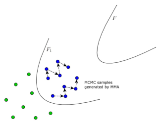
Figure 4: MCMC samples generated by the Modified Metropolis algorithm at the first conditional level of Subset Simulation.

Also assume that the corresponding system responses $y_{1}^{(1)}=g(x^{(1)}_{1}),\ldots,y^{(n)}_{1}=g(x^{(n)}_{1})$ are arranged in the decreasing order, i.e. $y_{1}^{(1)}\geq\ldots\geq y^{(n)}_{1}$. If the failure event $F$ is rare enough, that is if $p_{F}$ is sufficiently small, then it is very likely that none of the samples $x^{(1)}_{1},\ldots,x^{(n)}_{1}$ belongs to $F$, i.e. $y_{1}^{(i)}<y^{*}$ for all $i=1,\ldots,n$. Nevertheless, these MCMC samples can be used in the similar way the Monte Carlo samples $x^{(1)}_{0},\ldots,x^{(n)}_{0}$ were used.

By analogy with (20), define the second intermediate failure domain $F_{2}$ as follows:

$$F_{2}=\{x~{}:~{}g(x)>y_{2}^{*}\},$$ (36)

where

$$y_{2}^{*}=\frac{y_{1}^{(np)}+y_{1}^{(np+1)}}{2}.$$ (37)

Note that $y_{2}^{*}>y_{1}^{*}$ since $y_{1}^{(i)}>y_{1}^{*}$ for all $i=1,\ldots,n$. This means that $F\subset F_{2}\subset F_{1}$, and therefore, $F_{2}$ can be viewed as a conservative approximation to $F$ which is still rough, yet more accurate than $F_{1}$. Fig. 5 illustrates the definition of $F_{2}$.

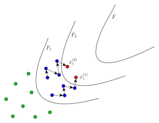
Figure 5: The second intermediate failure domain $F_{2}$. In this schematic illustration, $n=10$, $p=0.2$, so that there are exactly $np=2$ MCMC samples in $F_{2}$, $x_{1}^{(1)},x_{1}^{(2)}\in F_{2}$.

By construction, samples $x^{(1)}_{1},\ldots,x^{(np)}_{1}$ belong to $F_{2}$, while $x^{(np+1)}_{1},\ldots,x^{(n)}_{1}$ do not. As a result, the estimate for the conditional probability of $F_{2}$ given $F_{1}$ which is based on samples $x^{(1)}_{1},\ldots,x^{(n)}_{1}\sim\pi(\cdot|F_{1})$ is automatically equal to $p$,

$$\mathbb{P}(F_{2}|F_{1})\approx\frac{1}{n}\sum_{i=1}^{n}I_{F_{2}}(x^{(i)}_{1})=p.$$ (38)

Since $F\subset F_{2}\subset F_{1}$, the conditional probability $\mathbb{P}(F|F_{1})$ that appears in (23) can be expressed as a product:

$$\mathbb{P}(F|F_{1})=\mathbb{P}(F_{2}|F_{1})\mathbb{P}(F|F_{2}).$$ (39)

Combining (23) and (39) gives the following expression for the failure probability:

$$p_{F}=\mathbb{P}(F_{1})\mathbb{P}(F_{2}|F_{1})\mathbb{P}(F|F_{2}).$$ (40)

Thus, in view of (22) and (38), the problem of estimating $p_{F}$ is now reduced to estimating the conditional probability $\mathbb{P}(F|F_{2})$.

In the next step, as one may have already guessed, the Subset Simulation algorithm: populates $F_{2}$ by generating MCMC samples $x^{(1)}_{2},\ldots,x^{(n)}_{2}$ from $\pi(\cdot|F_{2})$ using the Modified Metropolis algorithm; defines the third intermediate failure domain $F_{3}\subset F_{2}$ such that $\mathbb{P}(F_{3}|F_{2})\approx\frac{1}{n}\sum_{i=1}^{n}I_{F_{3}}(x^{(i)}_{2})=p$ ; and reduces the original problem of estimating the failure probability $p_{F}$ to estimating the conditional probability $\mathbb{P}(F|F_{3})$ by representing $p_{F}=\mathbb{P}(F_{1})\mathbb{P}(F_{2}|F_{1})\mathbb{P}(F_{3}|F_{2})\mathbb{P}(F|F_{3})$. The algorithm proceeds in this way until the target failure domain $F$ has been sufficiently sampled so that the conditional probability $\mathbb{P}(F|F_{L})$ can be accurately estimated by $\frac{1}{n}\sum_{i=1}^{n}I_{F}(x^{(i)}_{L})$, where $F_{L}$ is the $L^{\mathrm{th}}$ intermediate failure domain, and $x^{(1)}_{L},\ldots,x^{(n)}_{L}\sim\pi(\cdot|F_{L})$ are the MCMC samples generated at the $L^{\mathrm{th}}$ conditional level. Subset Simulation can thus be viewed as a method that decomposes the rare failure event $F$ into a sequence of progressively “less-rare” nested events, $F\subset F_{L}\subset\ldots\subset F_{1}$, where all intermediate failure events $F_{1},\ldots,F_{L}$ are constructed adaptively by appropriately relaxing the value of the critical threshold $y_{1}^{*}<\ldots<y_{L}^{*}<y^{*}$.

V.3 Stopping criterion

In what follows, the stopping criterion for Subset Simulation is described in detail. Let $n_{F}(l)$ denote the number of failure samples at the $l^{\mathrm{th}}$ level, that is

$$n_{F}(l)=\sum_{i=1}^{n}I_{F}(x_{l}^{(i)}),$$ (41)

where $x_{l}^{(1)},\ldots,x_{l}^{(n)}\sim\pi(\cdot|F_{l})$. Since $F$ is a rare event, it is very likely that $n_{F}(l)=0$ for the first few conditional levels. As $l$ gets larger, however, $n_{F}(l)$ starts increasing since $F_{l}$, which approximates $F$ “from above”, shrinks closer to $F$. In general, $n_{F}(l)\geq n_{F}(l-1)$, since $F\subset F_{l}\subset F_{l-1}$ and the $np$ closest to $F$ samples among $x_{l-1}^{(1)},\ldots,x_{l-1}^{(n)}$ are present among $x_{l}^{(1)},\ldots,x_{l}^{(n)}$. At conditional level $l$, the failure probability $p_{F}$ is expressed as a product,

$$p_{F}=\mathbb{P}(F_{1})\mathbb{P}(F_{2}|F_{1})\ldots\mathbb{P}(F_{l}|F_{l-1})\mathbb{P}(F|F_{l}).$$ (42)

Furthermore, the adaptive choice of intermediate critical thresholds $y_{1}^{*},\ldots,y_{l}^{*}$ guarantees that the first $l$ factors in (42) approximately equal to $p$, and, thus,

$$p_{F}\approx p^{l}\cdot\mathbb{P}(F|F_{l}).$$ (43)

Since there are exactly $n_{F}(l)$ failure samples at the $l^{\mathrm{th}}$ level, the estimate of the last conditional probability in (42) which is based on samples $x_{l}^{(1)},\ldots,x_{l}^{(n)}\sim\pi(\cdot|F_{l})$ is given by

$$\mathbb{P}(F|F_{l})\approx\frac{1}{n}\sum_{i=1}^{n}I_{F}(x_{l}^{(i)})=\frac{n_{F}(l)}{n}.$$ (44)

If $n_{F}(l)$ is sufficiently large, i.e. the conditional event $(F|F_{l})$ is not rare, then the estimate (44) is fairly accurate. This leads to the following stopping criterion:

• If $\frac{n_{F}(l)}{n}\geq p$, i.e. there are at least $np$ failure samples among $x_{l}^{(1)},\ldots,x_{l}^{(n)}$, then Subset Simulation stops: the current conditional level $l$ becomes the last level, $L=l$, and the failure probability estimate derived from (43) and (44) is

  $$p_{F}\approx\hat{p}_{F}^{\mbox{\tiny{SS}}}=p^{L}\frac{n_{F}(L)}{n}.$$ (45)

• If $\frac{n_{F}(l)}{n}<p$, i.e. there are less than $np$ failure samples among $x_{l}^{(1)},\ldots,x_{l}^{(n)}$, then the algorithm proceeds by defining the next intermediate failure domain $F_{l+1}=\{x:g(x)>y_{l+1}^{*}\}$, where $y_{l+1}^{*}=(y_{l}^{(np)}+y_{l}^{(np+1)})/2$, and expressing $\mathbb{P}(F|F_{l})$ as a product $\mathbb{P}(F|F_{l})=\mathbb{P}(F_{l+1}|F_{l})\mathbb{P}(F|F_{l+1})\approx p\cdot\mathbb{P}(F|F_{l+1})$.

The described stopping criterion guarantees that the estimated values of all factors in the factorization $p_{F}=\mathbb{P}(F_{1})\mathbb{P}(F_{2}|F_{1})\ldots\mathbb{P}(F_{L}|F_{L-1})\mathbb{P}(F|F_{L})$ are not smaller than $p$. If $p$ is relatively large ($p=0.1$ is often used in applications), then it is likely that the estimates $\mathbb{P}(F_{1})\approx p$, $\mathbb{P}(F_{2}|F_{1})\approx p,\ldots,\mathbb{P}(F_{L}|F_{L-1})\approx p$, and $\mathbb{P}(F|F_{L})\approx\frac{n_{F}(L)}{n}(\geq p)$ are accurate even when the sample size $n$ is relatively small. As a result, the SS estimate (45) is also accurate in this case. This provides an intuitive explanation as to why Subset Simulation is efficient in estimating small probabilities of rare events. For a detailed discussion of error estimation for the SS method the reader is referred to SSbook .

V.4 Implementation details

In the rest of this section, the implementation details of Subset Simulation are discussed. The SS algorithm has two essential components that affect its efficiency: the parameter $p$ and the set of univariate proposal PDFs $\{q_{k}\}$, $k=1,\ldots,d$.

V.4.1 Level probability

The parameter $p$, called the level probability in SSbook and the conditional failure probability in BSS , governs how many intermediate failure domains $F_{l}$ are needed to reach the target failure domain $F$. As it follows form (45), a small value of $p$ leads to a fewer total number of conditional levels $L$. But at the same time, it results in a large number of samples $n$ needed at each conditional level $l$ for accurate determination of $F_{l}$ (i.e. determination of $y_{l}^{*}$) that satisfies $\frac{1}{n}\sum_{i=1}^{n}I_{F_{l}}(x^{(i)}_{l-1})=p$. In the extreme case when $p\leq p_{F}$, no levels are needed, $L=0$, and Subset Simulation reduces to the Direct Monte Carlo method. On the other hand, increasing the value of $p$ will mean that fewer samples are needed at each conditional level, but it will increase the total number of levels $L$. The choice of the level probability $p$ is thus a tradeoff between the total number of level $L$ and the number of samples $n$ at each level. In the original paper AuBeck , it has been found that the value $p=0.1$ yields good efficiency. The latter studies SSbook ; BSS , where the c.o.v. of the SS estimate $\hat{p}_{F}^{\mbox{\tiny{SS}}}$ has been analyzed, confirmed that $p=0.1$ is a nearly optimal value of the level probability.

V.4.2 Proposal distributions

The efficiency and accuracy of Subset Simulation also depends on the set of univariate proposal PDFs $\{q_{k}\}$, $k=1,\ldots,d$ that are used within the Modified Metropolis algorithm for sampling from the conditional distributions $\pi(\cdot|F_{l})$. To see this, note that in contract to the Monte Carlo samples $x_{0}^{(1)},\ldots,x_{0}^{(n)}\sim\pi(\cdot)$ which are i.i.d., the MCMC samples $x_{l}^{(1)},\ldots,x_{l}^{(n)}\sim\pi(\cdot|F_{l})$ are not independent for $l\geq 1$, since the MMA transition rule uses $x_{l}^{(i)}\sim\pi(\cdot|F_{l})$ to generate $x_{l}^{(i+1)}\sim\pi(\cdot|F_{l})$. This means that although these MCMC samples can be used for statistical averaging as if they were i.i.d., the efficiency of the averaging is reduced if compared with the i.i.d. case Doob . Namely, the more correlated $x_{l}^{(1)},\ldots,x_{l}^{(n)}$ are, the slower is the convergence of the estimate $P(F_{l+1}|F_{l})\approx\frac{1}{n}\sum_{i=1}^{n}I_{F_{l+1}}(x_{l}^{(i)})$, and, therefore, the less efficient it is. The correlation between samples $x_{l}^{(1)},\ldots,x_{l}^{(n)}$ is due to proposal PDFs $\{q_{k}\}$, which govern the generation of the next sample $x_{l}^{(i+1)}$ from the current one $x_{l}^{(i)}$. Hence, the choice of $\{q_{k}\}$ is very important.

It was observed in AuBeck that the efficiency of MMA is not sensitive to the type of the proposal PDFs (Gaussian, uniform, etc), however, it strongly depends on their spread (variance). Both small and large spreads tend to increase the correlation between successive samples. Large spreads may reduce the acceptance rate in (28), increasing the number of repeated MCMC samples. Small spreads, on the contrary, may lead to a reasonably high acceptance rate, but still produce very correlated samples due to their close proximity. As a rule of thumb, the spread of $q_{k}$, $k=1,\dots,d$, can be taken of the same order as the spread of the corresponding marginal PDF $\pi_{k}$ SSbook . For example, if $\pi$ is given by (18), so that all marginal PDFs are standard Gaussian, $\pi_{k}(x)=\phi(x)$, then all proposal PDFs can also be Gaussian with unit variance, $q_{k}(x|x_{k})=\phi(x-x_{k})$. This choice is found to give a balance between efficiency and robustness.

The spread of proposal PDFs can also be chosen adaptively. In BSS , where the problem of optimal scaling for the Modified Metropolis algorithm was studied in more detail, the following nearly optimal scaling strategy was proposed: at each conditional level, select the spread such that the the corresponding acceptance rate in (28) is between $30\%$ and $50\%$. In general, finding the optimal spread of proposal distributions is problem specific and a highly non-trivial task not only for MMA, but also for almost all MCMC algorithms.

VI Illustrative Examples

To illustrate Subset Simulation and to demonstrate its efficiency in estimating small probabilities of rare failure events, two examples are considered in this section. As it has been discussed in Section II, in reliability problems, the dimension $d$ of the input space $\mathcal{X}$ is usually very large. In spite of this, for visualization and educational purposes, a linear reliability problem in two dimensions ($d=2$) is first considered in Section VI.1. A more realistic high-dimensional example ($d=10^{3}$) is considered in the subsequent Section VI.2.

VI.1 Subset Simulation in 2-D

Suppose that $d=2$, i.e. the response variable $y$ depends only on two input variables $x_{1}$ and $x_{2}$. Consider a linear performance function,

$$g(x_{1},x_{2})=x_{1}+x_{2},$$ (46)

where $x_{1}$ and $x_{2}$ are independent standard Gaussian, $x_{i}\sim\mathcal{N}(0,1)$, $i=1,2.$ The failure domain $F$ is then a half-plane defined by

$$F=\{(x_{1},x_{2})~{}:~{}x_{1}+x_{2}>y^{*}\}.$$ (47)

In this example, the failure probability $p_{F}$ can be calculated analytically. Indeed, since $x_{1}+x_{2}\sim\mathcal{N}(0,2)$, and, therefore, $\frac{x_{1}+x_{2}}{\sqrt{2}}\sim\mathcal{N}(0,1)$,

$$\begin{split}p_{F}&=\mathbb{P}(x_{1}+x_{2}>y^{*})=\mathbb{P}\left(\frac{x_{1}+x_{2}}{\sqrt{2}}>\frac{y^{*}}{\sqrt{2}}\right)\\ &=1-\Phi\left(\frac{y^{*}}{\sqrt{2}}\right),\end{split}$$ (48)

where $\Phi$ is the standard Gaussian CDF. This expression for the failure probability can be used as a check on the SS estimate. Moreover, expressing $y^{*}$ in terms of $p_{F}$,

$$y^{*}=\sqrt{2}\Phi^{-1}(1-p_{F}),$$ (49)

allows to solve the inverse problem, namely, to formulate a linear reliability problem with a given value of the failure probability. Suppose that $p_{F}=10^{-10}$ is the target value. Then the corresponding value of the critical threshold is $y^{*}\approx 9$.

Subset Simulation were used to estimate the failure probability of the rare event (47) with $y^{*}=9$. The parameters of the algorithm were chosen as follows: the level probability $p=0.1$, the proposal PDFs $q_{k}(x|x_{k})=\phi(x-x_{k})$, and the sample size $n=10^{3}$ per each level. This implementation of SS led to $L=9$ conditional levels, making the total number of generated samples $N=n+L(n-np)=9.1\times 10^{3}$. The obtained SS estimate is $\hat{p}_{F}^{\mbox{\tiny{SS}}}=1.58\times 10^{-10}$ which is quite close to the true value $p_{F}=10^{-10}$. Note that, in this example, it is hopeless to obtain an accurate estimate by the Direct Monte Carlo method since the DMC estimate (12) based on $N=9.1\times 10^{3}$ samples is effectively zero: the rare event $F$ is too rare.

Fig. 6 shows the samples generated by the SS method. The dashed lines represent the boundaries of intermediate failure domains $F_{l}$, $l=1,\ldots,L=9$. The solid line is the boundary of the target failure domain $F$. This illustrates how Subset Simulation pushes Monte Carlo samples (red) towards the failure region.

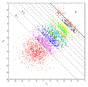
Figure 6: Samples generated by Subset Simulation: red samples are Monte Carlo samples generated at the $0^{\mathrm{th}}$ unconditional level, purple sample are MCMC sample generated at the $1^{\mathrm{st}}$ conditional level, etc. The dashed lines represent the boundaries of intermediate failure domains $F_{l}$, $l=1,\ldots,L=9$. The solid line is the boundary of the target failure domain $F$. [Example 6.1].

VI.2 Subset Simulation in High Dimensions

It is straightforward to generalize the low-dimensional example considered in the previous section to high dimensions. Consider a linear performance function

$$g(x)=\sum_{i=1}^{d}x_{i},$$ (50)

where $x_{1},\ldots,x_{d}$ are i.i.d. standard Gaussian. The failure domain is then a half-space defined by

$$F=\{x~{}:~{}\sum_{i=1}^{d}x_{i}>y^{*}\}.$$ (51)

In this example, $d=10^{3}$ is considered, hence the input space $\mathcal{X}=\mathbb{R}^{d}$ is indeed high-dimensional. As before, the failure probability can be calculated analytically:

$$\begin{split}p_{F}&=\mathbb{P}\left(\sum_{i=1}^{d}x_{i}>y^{*}\right)=\mathbb{P}\left(\frac{\sum_{i=1}^{d}x_{i}}{\sqrt{d}}>\frac{y^{*}}{\sqrt{d}}\right)\\ &=1-\Phi\left(\frac{y^{*}}{\sqrt{d}}\right).\end{split}$$ (52)

This expression will be used as a check on the SS estimate.

First, consider the following range of values for the critical threshold, $y^{*}\in[0,200]$. Fig. 7 plots $y^{*}$ versus $p_{F}$.

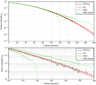
Figure 7: Critical threshold $y^{*}$ versus the failure probability $p_{F}$. [Example 6.2].

The solid red curve corresponds to the sample mean of the SS estimates $\hat{p}_{F}^{\mbox{\tiny{SS}}}$ which is based on $100$ independent runs of Subset Simulation. The two dashed red curves correspond to the sample mean $\pm$ one sample standard deviation. The SS parameters were set as follows: the level probability $p=0.1$, the proposal PDFs $q_{k}(x|x_{k})=\phi(x-x_{k})$, and the sample size $n=3\times 10^{3}$ per each level. The solid blue curve (which almost coincides with the solid red curve) corresponds to the true values of $p_{F}$ computed from (52). The dark green curves correspond to Direct Monte Carlo: the solid curve is the sample mean (based on 100 independent runs) of the DMC estimates $\hat{p}_{F}^{\mbox{\tiny{DMC}}}$ (12), and the two dashed curves are the sample mean $\pm$ one sample standard deviation. The total number of samples $N$ used in DMC equals to the average (based on 100 runs) total number of samples used in SS. Finally, the dashed light green curves show the theoretical performance of Direct Monte Carlo, namely, they correspond to the true value of $p_{F}$ (52) $\pm$ one theoretical standard deviation obtained from (14). The bottom panel of Fig. 7 shows the zoomed in region that corresponds to the values $y^{*}\in[100,160]$ of the critical threshold. Note that for relatively large values of the failure probability, $p_{F}<10^{-3}$, both DMC and SS produce accurate estimates of $p_{F}$. For smaller values however, $p_{F}<10^{-5}$, the DMC estimate starts to degenerate, while SS still accurately estimates $p_{F}$. This can be seen especially well in the bottom panel of the figure.

The performances of Subset Simulation and Direct Monte Carlo can be also compared in terms of the coefficient of variation of the estimates $\hat{p}_{F}^{\mbox{\tiny{SS}}}$ and $\hat{p}_{F}^{\mbox{\tiny{DMC}}}$. This comparison is shown in Fig. 8.

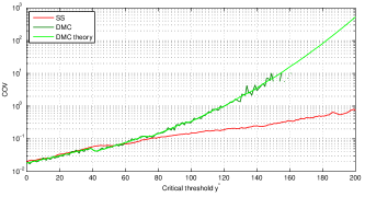
Figure 8: Critical threshold $y^{*}$ versus the c.o.v. [Example 6.2].

The red and dark green curves represent the sample c.o.v. for SS and DMC, respectively. The light green curve is the theoretical c.o.v. of $\hat{p}_{F}^{\mbox{\tiny{DMC}}}$ given by (15). When the critical threshold is relatively small $y^{*}<60$, the performances of SS and DMC are comparable. As $y^{*}$ gets large, the c.o.v. of $\hat{p}_{F}^{\mbox{\tiny{DMC}}}$ starts to grow much faster than that of $\hat{p}_{F}^{\mbox{\tiny{SS}}}$. In other words, SS starts to outperform DMC, and the larger $y^{*}$, i.e. the more rare the failure event, the more significant the outperformance is.

The average total number of samples used in Subset Simulation versus the corresponding values of failure probability is shown in the top panel of Fig. 9.

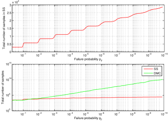
Figure 9: Failure probability versus the total number of samples. [Example 6.2].

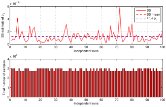
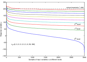
Figure 10: Performance of Subset Simulation for 100 independent runs. The critical threshold is $y^{*}=200$, the corresponding true value of the failure probability is $p_{F}=1.27\times 10^{-10}$. [Example 6.2].

Figure 11: System responses $y_{l}^{(1)}\geq\ldots\geq y_{l}^{(n)}$, $n=3\times 10^{3}$, for all levels, $l=0,\ldots,L=9$, for a fixed simulation run. [Example 6.2].

The staircase nature of the plot is due to the fact that every time when $p_{F}$ crosses the value $p^{k}$ by decreasing from $p^{k}+\epsilon$ to $p^{k}-\epsilon$, an additional conditional level is required. In this example, $p=0.1$ is used, that why the jumps occur at $p_{F}=10^{-k}$, $k=1,2,\ldots$. The jumps are more pronounced for larger values of $p_{F}$, where the SS estimate is more accurate. For smaller values of $p_{F}$, where the SS estimate is less accurate, the jumps are more smoothed out by averaging over independent runs.

In Fig. 8, where the c.o.v’s of SS and DMC are compared, the total numbers of samples (computational efforts) used in the two methods are the same. The natural question is then the following: by how much should the total number of samples $N$ used in DMC be increased to achieve the same c.o.v as in SS (so that the green curve in Fig. 8 coincides with the red curve)? The answer is given in the bottom panel of Fig. 9. For example, if $p_{F}=10^{-10}$, then $N=10^{10}$, while the computational effort of SS is less than $10^{5}$ samples.

Simulation results presented in Figures 7,8, and 9 clearly indicate that (a) Subset Simulation produces a relatively accurate estimate of the failure probability, and (b) Subset Simulation drastically outperforms Direct Monte Carlo when estimating probabilities of rare events.

Let us now focus on a specific value of the critical threshold, $y^{*}=200$, which corresponds to a very rare failure event (51) with probability $p_{F}=1.27\times 10^{-10}$. Fig. 11 demonstrates the performance of Subset Simulation for 100 independent runs. The top panel shows the obtained SS estimate $\hat{p}_{F}^{\mbox{\tiny{SS}}}$ for each run. Although $\hat{p}_{F}^{\mbox{\tiny{SS}}}$ varies significantly (its c.o.v. is $\delta(\hat{p}_{F}^{\mbox{\tiny{SS}}})=0.74$), its mean value $\overline{\hat{p}_{F}^{\mbox{\tiny{SS}}}}=1.18\times 10^{-10}$ (dashed red line) is close to the true value of the failure probability (dashed blue line). The bottom panel shows the total number of samples used in SS in each run. It is needless to say that the DMC estimate based on $N\sim 3\times 10^{4}$ samples would almost certainly be zero.

Fig. 11 shows the system responses $y_{l}^{(1)}\geq\ldots\geq y_{l}^{(n)}$, $n=3\times 10^{3}$, for all levels, $l=0,\ldots,L=9$, for a fixed simulation run. As expected, for the first few levels (6 levels in this case), the number of failure samples $n_{F}(l)$, i.e. samples $x_{l}^{(i)}$ with $y_{l}^{(i)}=g(x_{l}^{(i)})>y^{*}$, is zero. As Subset Simulation starts pushing the samples towards the failure domain, $n_{F}(l)$ starts increasing with $n_{F}(6)=3$, $n_{F}(7)=6$, $n_{F}(8)=59$, and, finally, $n_{F}(9)=582$, after which the algorithm stopped since $n_{F}(9)/n=0.194$ which is large than $p=0.1$. Finally, Fig. 12 plots the intermediate (relaxed) critical thresholds $y^{*}_{1},\ldots,y^{*}_{L}$ at different levels obtained in a fixed simulation run.

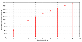
Figure 12: Intermediate critical thresholds $y^{*}_{1},\ldots,y^{*}_{L}$, $L=9$, at different conditional levels in a fixed simulation run. [Example 6.2].

VII MATLAB code

This section contains the MATLAB code for the examples considered in Section VI. For educational purposes, the code was written as readable as possible with numerous comments. As a result of this approach, the efficiency of the code was unavoidably scarified. This code is also available online at http://arxiv.org/.

⬇

1% Subset Simulation for Liner Reliability Problem

2% Performance function: g(x)=x1+...+xd

3% Input variables x1,...,xd are i.i.d. N(0,1)

4% Written by K.M. Zuev, Institute of Risk & Uncertainty, Uni of Liverpool

5%------------------------------------------------------------------------

6clear;

7d=1000; % dimension of the input space

8YF=200; % critical threshold (failure <=> g(x)>YF)

9pF=1-normcdf(YF/sqrt(d)); % true value of the failure probability

10n=3000; % number of samples per level

11p=0.1; % level probability

12nc=n*p; % number of Markov chains

13ns=(1-p)/p; % number of states in each chain

14%------------------------------------------------------------------------

15L=0; % current (unconditional) level

16x=randn(d,n); % Monte Carlo samples

17nF=0; % number of failure samples

18for i=1:n

19 y(i)=sum(x(:,i)); % system response y=g(x)

20 if y(i)>YF % y(i)>YF <=> x(:,i) is a failure sample

21 nF=nF+1;

22 end

23end

24while nF(L+1)/n<p % stopping criterion

25 L=L+1; % next conditional lelvel is needed

26 [y(L,:),ind]=sort(y(L,:),'descend'); % renumbered responses

27 x(:,:,L)=x(:,ind(:),L); % renumbered samples

28 Y(L)=(y(L,nc)+y(L,nc+1))/2; % L^th intermediate threshold

29 z(:,:,1)=x(:,1:nc,L); % Markov chain "seeds"

30 %--------------------------------------------------------------------

31 % Modified Metropolis algorithm for sampling from pi(x|F_L)

32 for j=1:nc

33 for m=1:ns

34 % Step 1:

35 for k=1:d

36 a=z(k,j,m)+randn; % Step 1(a)

37 r=min(1,normpdf(a)/normpdf(z(k,j,m))); % Step 1(b)

38 % Step 1(c):

39 if rand<r

40 q(k)=a;

41 else

42 q(k)=z(k,j,m);

43 end

44 end

45 % Step 2:

46 if sum(q)>Y(L) % q belongs to F_L

47 z(:,j,m+1)=q;

48 else

49 z(:,j,m+1)=z(:,j,m);

50 end

51 end

52 end

53 for j=1:nc

54 for m=1:ns+1

55 x(:,(j-1)*(ns+1)+m,L+1)=z(:,j,m); % samples from pi(x|F_L)

56 end

57 end

58 clear z;

59 %--------------------------------------------------------------------

60 nF(L+1)=0;

61 for i=1:n

62 y(L+1,i)=sum(x(:,i,L+1)); % system response y=g(x)

63 if y(L+1,i)>YF % then x(:,i,L+1) is a failure sample

64 nF(L+1)=nF(L+1)+1; % number of failure samples at level L+1

65 end

66 end

67end

68pF_SS=p^(L)*nF(L+1)/n; % SS estimate

69N=n+n*(1-p)*(L); % total number of samples

70%------------------------------------------------------------------------

VIII Summary

In this paper, a detailed exposition of Subset Simulation, an advanced stochastic simulation method for estimation of small probabilities of rare events, is provided at introductory level. A simple step-by-step derivation of Subset Simulation is given, and important implementation details are discussed. The method is illustrated with a few intuitive examples.

After the original paper AuBeck was published, various modifications of SS were proposed: SS with splitting ChingAuBeck , Hybrid SS ChingBeckAu , and Two-Stage SS KatafygiotisCheung , to name but a few. It is important to highlight, however, that none of these modifications offer a drastic improvement over the original algorithm. A Bayesian analog of SS was developed in BSS . For further reading on Subset Simulation and its applications, a fundamental and very accessible monograph SSbook is strongly recommended, where the method is presented from the CCDF (complementary cumulative distribution function) perspective and where the error estimation is discussed in detail.

Also, it is important to emphasize that Subset Simulation provides an efficient solution for general reliability problems without using any specific information about the dynamic system other than an input output model. This independence of a system s inherent properties makes Subset Simulation potentially useful for applications in different areas of science and engineering.

As a final remark, it is a pleasure to thank Professor Siu-Kui Au whose comments on the first draft of the paper were very helpful, Professor James Beck, who generously shared his knowledge of and experience with Subset Simulation, and Professor Francis Bonahon for general support and for creating a nice atmosphere at the Department of Mathematics of the University of Southern California, where the author started this work.

References

- (1) Au, S. K., Beck, J. L. (2001). Estimation of small failure probabilities in high dimensions by subset simulation. Probabilistic Engineering Mechanics, 16(4), 263 277.
- (2) Au, S. K., Beck, J. L. (2001). First-excursion probabilities for linear systems by very efficient importance sampling. Probabilistic Engineering Mechanics, 16(3), 193 207.
- (3) Au, S. K., Wang, Y. (2014). Engineering risk assessment and design with subset simulation. John Wiley Sons, Singapore. To appear.
- (4) Bucher, C. (1990). A fast and efficient response surface approach for structural reliability problem. Structural Safety, 7, 57-66.
- (5) Ching, J., Au, S. K., Beck, J. L. (2005). Reliability estimation of dynamical systems subject to stochastic excitation using subset simulation with splitting, Computer Methods in Applied Mechanics and Engineering, 194(12-16), 1557-1579.
- (6) Ching, J., Beck, J. L., Au, S. K. (2005). Hybrid subset simulation method for reliability estimation of dynamical systems subject to stochastic excitation, Probabilistic Engineering Mechanics, 20(3), 199-214.
- (7) Ditlevsen, O., Madsen, H. O. (1996). Structural Reliability Methods. Chichester: John Wiley Sons.
- (8) Doob, J. L. (1953). Stochastic processes. New York: Wiley.
- (9) Engelund, S., Rackwitz, R. (1993). A benchmark study on importance sampling techniques in structural reliability. Structural Safety, 12(4), 255 276.
- (10) Faravelli, L. (1989). Response-surface approach for reliability analysis. Journal of the Engineering Mechanics, 115,2763 81.
- (11) Grooteman, F. (2008). Adaptive radial-based importance sampling method for structural reliability. Structural Safety, 30(6), 533 542.
- (12) Hurtado, J.E., Alvarez, D.A. (2003). A classification approach for reliability analysis with stochastic finite element modeling. Journal of Structural Engineering, 129(8), 1141 1149.
- (13) Hurtado, J.E. (2004). Structural reliability. Statistical learning perspectives. Heidelberg: Springer.
- (14) Katafygiotis, L. S., Cheung, S. H. (2005). A two-stage subset simulation-based approach for calculating the reliability of inelastic structural systems subjected to Gaussian random excitations, Computer Methods in Applied Mechanics and Engineering, 194(12-16), 1581-1595.
- (15) Katafygiotis, L. S, Moan, T., Cheung, S. H. (2007). Auxiliary domain method for solving multi-objective dynamic reliability problems for nonlinear structures. Structural Engineering Mechanics, 25(3), 347 363.
- (16) Katafygiotis, L. S., Zuev, K. M. (2007). Estimation of small failure probabilities in high dimensions by adaptive linked importance sampling. Proc. COMPDYN-2007.
- (17) Koutsourelakis, P. S., Pradlwarter, H. J., Schuëller, G. I. (2004). Reliability of structures in high dimensions, part I: algorithms and applications. Probabilistic Engineering Mechanics, 19(4), 409 417.
- (18) Liu, J. S. (2001). Monte Carlo strategies is scientific computing. New York: SpringerVerlag.
- (19) Madsen, H. O., Krenk, S., Lind, N. C. (2006). Methods of structural safety. Dover Publications, Inc., Mineola, N.Y.
- (20) Melchers, R. (1999). Structural reliability analysis and prediction. Chichester: John Wiley Sons.
- (21) Metropolis, N. (1987). The beginning of the Monte Carlo method. Los Alamos Science, 15, 125-130.
- (22) Metropolis, N., Ulam, S. (1949). The Monte Carlo method, Journal of the American Statistical Association, 44, 335-341.
- (23) Metropolis, N., Rosenbluth A. W., Rosenbluth M. N., Teller A.H., Teller E. (1953). Equation of state calculations by fast computing machines. J. Chem. Phys. 21(6), 1087 1092.
- (24) Nataf, A. (1962). Détermination des distributions de probabilité dont les marges sont donées. Comptes Rendues de l’Académie des Sciences, 225, 42-43.
- (25) Papadrakakis, M., Papadopoulos, V., Lagaros, N. D. (1996). Structural reliability analysis of elastic plastic structures using neural networks and Monte Carlo simulation. Computer Methods in Applied Mechanics and Engineering, 136, 145 63.
- (26) Robert, C. P., Casella, G. (2004). Monte Carlo statistical methods. New York: Springer-Verlag.
- (27) Rosenblatt, M. (1952). Remarks on a multivariate transformation. The Annals of Mathematical Statistics, 23, 470-472.
- (28) Schuëller, G. I., Bucher, C. G., Bourgund, U., Ouypornprasert, W. (1989). On efficient computational schemes to calculate structural failure probabilities. Probabilistic Engineering Mechanics, 4(1), 10-18.
- (29) Zuev, K. M., Beck, J. L., Au. S. K., Katafygiotis, L. S. (2012). Bayesian post-processor and other enhancements of Subset Simulation for estimating failure probabilities in high dimensions. Computers Structures, 92-93, 283-296.
- (30) Zuev, K. M., Katafygiotis, L. S. (2011). Horseracing Simulation algorithm for evaluation of small failure probabilities. Probabilistic Engineering Mechanics, 26(2), 157 164.