Loop-corrected belief propagation for lattice spin models

Abstract

Belief propagation (BP) is a message-passing method for solving probabilistic graphical models. It is very successful in treating disordered models (such as spin glasses) on random graphs. On the other hand, finite-dimensional lattice models have an abundant number of short loops, and the BP method is still far from being satisfactory in treating the complicated loop-induced correlations in these systems. Here we propose a loop-corrected BP method to take into account the effect of short loops in lattice spin models. We demonstrate, through an application to the square-lattice Ising model, that loop-corrected BP improves over the naive BP method significantly. We also implement loop-corrected BP at the coarse-grained region graph level to further boost its performance.

1 Introduction

Belief propagation (BP) is a message-passing method for solving probabilistic graphical models. It was developed in the computer science research field Pearl-1988 and, independently, also in the statistical physics field along with the replica-symmetric mean field theory Mezard-etal-1987 . For spin glass physicists the BP method is commonly referred to as the replica-symmetric cavity method. The basic physical idea behind BP is the Bethe-Peierls approximation Bethe-1935 ; Peierls-1936a ; Chang-1937 , which assumes that if a vertex is deleted from a graph, all of its nearest neighboring vertices will become completely uncorrelated in the remaining (cavity) graph. BP has good quantitative predicting power if the graph’s characteristic loop length is much longer than the system’s typical correlation length.

The BP method is exact for models defined on a tree graph which contains no loops. A finite-connectivity random graph contains many loops, but the typical loop length increases logarithmically with the total number of vertices in the graph, and BP also performs excellently on sufficiently large random-graph systems. A lot of random combinatorial optimization problems and random-graph spin glass models have been successfully solved by BP and the replica-symmetric mean field theory during the last two decades Mezard-Montanari-2009 .

Finite-dimensional lattice models have an abundant number of short loops, which cause complicated local correlations in the system. The correlation length of the system at sufficiently low temperatures often exceeds the characteristic length of short loops. At the moment, BP is still far from being satisfactory in treating the complicated loop-induced local correlations in these systems. In recent years the generalized belief propagation (GBP), as a promising way of overcoming the naive BP’s shortcomings, has been seriously explored Yedidia-Freeman-Weiss-2005 ; Pelizzola-2005 ; Rizzo-etal-2010 ; Wang-Zhou-2013 ; LageCastellanos-Mulet-RicciTersenghi-2014 . The GBP method is rooted in the cluster variational method Kikuchi-1951 ; An-1988 and it abandons the Bethe-Peierls approximation.

Here we explore a simple way of improving BP while still keeping the Bethe-Peierls approximation. We propose a loop-corrected BP method to take into account the effect of short loops in lattice spin models. The loop-corrected BP method, as a hierarchical approximation scheme, is conceptually straightforward to understand, and its numerical implementation appears to be easier than the GBP method. As a proof of principle, we apply loop-corrected BP to the square-lattice Ising model for which exact results are available, and demonstrate that it indeed significantly outperforms the naive BP. We also implement loop-corrected BP at the coarse-grained region graph level Zhou-Wang-2012 to further boost its performance. Our numerical results on the square-lattice Ising model indicate that loop-corrected BP might be a preferred method than GBP.

The actual applications of loop-corrected BP to the Edwards-Anderson spin glass model Edwards-Anderson-1975 on the square lattice and especially on the three-dimensional cubic lattice will be carried out in a follow-up paper. As potential practical applications, we suggest that loop-corrected BP might be useful in two-dimensional image processing tasks, such as image recovery Nishimori-2001 .

For reason of clarity, in the remaining part of this paper we describe the loop-corrected BP method using the square lattice as a representative example.

Let us finish the Introduction by noting that loop correction to BP has been a focusing issue in the last decade and various protocols have been investigated Montanari-Rizzo-2005 ; Parisi-Slanina-2006 ; Chertkov-Chernyak-2006b ; Mooij-etal-2007 ; Bulatov-2008 ; Xiao-Zhou-2011 ; Zhou-Wang-2012 ; Ravanbakhsh-Yu-Greiner-2012 ). For example, the proposal of Mooij and co-authors Mooij-etal-2007 (see also Ravanbakhsh-Yu-Greiner-2012 ) considers the correlations among the neighboring vertices of a given focal vertex by computing the joint distribution of all these neighboring vertices’ spin states. This proposal abandons the Bethe-Peierls approximation and it is computationally expensive, while its performance on square-lattice spin models seems to be inferior to that of the conventional cluster variational method Mooij-etal-2007 . Another interesting approach Bulatov-2008 is based on the self-avoiding walk tree representation of a loopy graph Weitz-2006 and its full potential is yet to be explored.

2 The lattice spin system

Let us consider a periodic square lattice $G$ of width $L$ containing $N=L\times L$ vertices, see Fig. 1 (the numerical results shown in Fig. 3 and Fig. 6 correspond to $L=\infty$). Each vertex $m\in\{1,2,\ldots,N\}$ of this lattice has a spin state $\sigma_{m}\in\{-1,+1\}$ and it interacts with its four nearest neighboring vertices. The interaction between two vertices $m$ and $n$ is represented by an edge in the lattice and this edge is denoted as $\langle m,n\rangle$ in our following discussions. The set formed by all the nearest neighboring vertices of vertex $m$ is denoted as $\partial m$, i.e., $\partial m\equiv\{n\,:\,\langle m,n\rangle\in G\}$. For the particular example of Fig. 1, $\partial m=\{l,h,n,r\}$ and $\partial n=\{m,i,o,s\}$. In addition, we denote by $\partial m\backslash n$ the set obtained by deleting vertex $n$ from the set $\partial m$, e.g., $\partial m\backslash n=\{l,h,r\}$ and $\partial n\backslash m=\{i,o,s\}$.

We denote a microscopic spin configuration of the whole lattice $G$ as $\underline{\sigma}$, that is, $\underline{\sigma}\equiv\{\sigma_{1},\sigma_{2},\ldots,\sigma_{N}\}$. The energy for each of the $2^{N}$ possible microscopic configurations is defined as

$$E(\underline{\sigma})=-\sum\limits_{i\in G}h^{0}_{i}\sigma_{i}-\sum\limits_{\langle i,j\rangle\in G}J_{ij}\sigma_{i}\sigma_{j}\;,$$ (1)

where $h^{0}_{i}$ is the local external field on vertex $i$, and $J_{ij}$ is the spin coupling constant of the edge $\langle i,j\rangle$. In the limiting case of $J_{ij}=+J$ for all the edges, this model is the ferromagnetic Ising model Ising-1925 . In the other limiting case of the Edwards-Anderson spin glass model, each edge coupling constant $J_{ij}$ is set to be $+J$ or $-J$ with equal probability and independently of all the other coupling constants Edwards-Anderson-1975 . In the numerical calculations of this paper we choose the energy unit to be $J$, which is equivalent to setting $J=1$.

Let us denote by $\mathcal{S}$ a macroscopic equilibrium state of the system at a given temperature $T$. When $T$ is sufficiently high the system has only a single macroscopic state, then $\mathcal{S}$ contains all the $2^{N}$ microscopic configurations. At certain critical temperature value $T_{c}$ an ergodicity-breaking transition may occur in the configuration space of the system, then the system at $T<T_{c}$ has two or even many macroscopic states, each of which containing a subset of the $2^{N}$ microscopic configurations Huang-1987 that are mutually reachable through a chain of local spin flips.

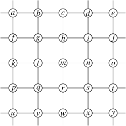
Figure 1: The square lattice $G$ with periodic boundary conditions. There are $L$ (here $L=5$) vertices on each boundary line, and the total number of vertices is $N=L\times L$.

3 The Bethe-Peierls approximation and the belief-propagation equation

We now briefly review the BP method. Within a macroscopic equilibrium state $\mathcal{S}$, the marginal probability distribution $q_{m}(\sigma_{m})$ for the spin state of a single vertex $m$ is defined as

$$q_{m}(\sigma)=\frac{\sum_{\underline{\sigma}}^{\prime}\delta_{\sigma_{m}}^{\sigma}e^{-\beta E(\underline{\sigma})}}{\sum_{\underline{\sigma}}^{\prime}e^{-\beta E(\underline{\sigma})}}\;,$$ (2)

where $\delta_{\sigma}^{\tilde{\sigma}}$ is the Kronecker symbol such that $\delta_{\sigma}^{\tilde{\sigma}}=1$ if $\sigma=\tilde{\sigma}$ and $\delta_{\sigma}^{\tilde{\sigma}}=0$ if $\sigma\neq\tilde{\sigma}$; $\beta\equiv 1/T$ is the inverse temperature; the superscript ^′ of the summation symbol means that the summation is over all the microscopic configurations $\underline{\sigma}$ belonging to the macroscopic state $\mathcal{S}$.

Since vertex $m$ interacts only with the vertices in $\partial m$, we divide the total energy $E(\underline{\sigma})$ into two parts:

$$E(\underline{\sigma})=\Bigl{[}-h^{0}_{m}\sigma_{m}-\sum\limits_{n\in\partial m}J_{mn}\sigma_{m}\sigma_{n}\Bigr{]}+E_{\backslash m}(\underline{\sigma}_{\backslash m})\;,$$ (3)

where $E_{\backslash m}(\underline{\sigma}_{\backslash m})$ is the total energy of the cavity lattice $G_{\backslash m}$ formed by deleting vertex $m$ from the original lattice $G$ (see Fig. 2):

$$E_{\backslash m}(\underline{\sigma}_{\backslash m})=-\sum\limits_{i\in G_{\backslash m}}h^{0}_{i}\sigma_{i}-\sum\limits_{\langle i,j\rangle\in G_{\backslash m}}J_{ij}\sigma_{i}\sigma_{j}\;,$$ (4)

and $\underline{\sigma}_{\backslash m}\equiv\{\sigma_{j}\,:\,j\in G_{\backslash m}\}$. After inserting Eq. (3) into Eq. (2), we obtain that

$$q_{m}(\sigma)=\frac{e^{\beta h^{0}_{m}\sigma}\sum\limits_{\underline{\sigma}_{\partial m}}q_{\backslash m}(\underline{\sigma}_{\partial m})\prod\limits_{n\in\partial m}e^{\beta\sigma J_{mn}\sigma_{n}}}{\sum\limits_{\sigma_{m}}e^{\beta h^{0}_{m}\sigma_{m}}\sum\limits_{\underline{\sigma}_{\partial m}}q_{\backslash m}(\underline{\sigma}_{\partial m})\prod\limits_{n\in\partial m}e^{\beta\sigma_{m}J_{mn}\sigma_{n}}}\;,$$ (5)

where $\underline{\sigma}_{\partial m}\equiv\{\sigma_{n}:n\in\partial m\}$ denotes a microscopic spin configuration of the vertices in set $\partial m$, and $q_{\backslash m}(\underline{\sigma}_{\partial m})$ is the probability distribution of $\underline{\sigma}_{\partial m}$ within the macroscopic equilibrium state $\mathcal{S}$ of the cavity lattice $G_{\backslash m}$:

$$q_{\backslash m}(\underline{\sigma}_{\partial m})\equiv\frac{\sum_{\underline{\tilde{\sigma}}_{\backslash m}}^{\prime}e^{-\beta E_{\backslash m}(\underline{\tilde{\sigma}}_{\backslash m})}\prod_{n\in\partial m}\delta_{\tilde{\sigma}_{n}}^{\sigma_{n}}}{\sum_{\underline{\tilde{\sigma}}_{\backslash m}}^{\prime}e^{-\beta E_{\backslash m}(\underline{\tilde{\sigma}}_{\backslash m})}}\;.$$ (6)

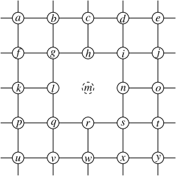
Figure 2: The square lattice $G_{\backslash m}$ obtained by deleting vertex $m$ (and all its attached edges) from the lattice $G$ of Fig. 1. Such a lattice is referred to as a cavity lattice.

Since vertex $m$ is absent in the cavity lattice $G_{\backslash m}$, one expects that the correlations among the vertices of set $\partial m$ are much weaker in $G_{\backslash m}$ than in the original lattice $G$. Following the idea of Bethe and Peierls Bethe-1935 ; Peierls-1936a , let us neglecting all the remaining correlations among the vertices of $\partial m$ in $G_{\backslash m}$ and approximate $q_{\backslash m}(\underline{\sigma}_{\partial m})$ by the following factorized form:

$$q_{\backslash m}(\underline{\sigma}_{\partial m})\approx\prod\limits_{n\in\partial m}q_{n\backslash m}(\sigma_{n})\;,$$ (7)

where $q_{n\backslash m}(\sigma_{n})$ is the marginal probability distribution of the spin state of vertex $n$ in the cavity lattice $G_{\backslash m}$. Inserting Eq. (7) into Eq. (5) we obtain the following approximate expression for $q_{m}(\sigma_{m})$:

$$q_{m}(\sigma)=\frac{e^{\beta h^{0}_{m}\sigma}\prod\limits_{n\in\partial m}\Bigl{[}\sum\limits_{\sigma_{n}}e^{\beta\sigma J_{mn}\sigma_{n}}q_{n\backslash m}(\sigma_{n})\Bigr{]}}{\sum\limits_{\sigma_{m}}e^{\beta h^{0}_{m}\sigma_{m}}\prod\limits_{n\in\partial m}\Bigl{[}\sum\limits_{\sigma_{n}}e^{\beta\sigma_{m}J_{mn}\sigma_{n}}q_{n\backslash m}(\sigma_{n})\Bigr{]}}\;.$$ (8)

Similar to Eq. (8), we can apply the Bethe-Peierls approximation on the cavity lattice $G_{\backslash m}$ to compute the marginal probability distribution $q_{n\backslash m}(\sigma_{m})$ of vertex $n$:

$$q_{n\backslash m}(\sigma)=\frac{e^{\beta h^{0}_{n}\sigma}\prod\limits_{i\in\partial n\backslash m}\Bigl{[}\sum\limits_{\sigma_{i}}e^{\beta\sigma J_{ni}\sigma_{i}}q_{i\backslash n}(\sigma_{i})\Bigr{]}}{\sum\limits_{\sigma_{n}}e^{\beta h^{0}_{n}\sigma_{n}}\prod\limits_{i\in\partial n\backslash m}\Bigl{[}\sum\limits_{\sigma_{i}}e^{\beta\sigma_{n}J_{ni}\sigma_{i}}q_{i\backslash n}(\sigma_{i})\Bigr{]}}\;.$$ (9)

The above equation is referred to as a belief-propagation equation in the literature Pearl-1988 . The BP equation is a self-consistent equation. We can iterate Eq. (9) on all the edges of the lattice $G$ and, if this iteration reaches a fixed point, then use Eq. (8) to compute the mean spin value of any given vertex $m$ in the lattice.

The above-mentioned mean field theory is very successful in quantitatively predicting the properties of spin models on random finite-connectivity graphs ZhouBook . However, when applied on the square-lattice Ising model with no external field, it predicts a transition between the paramagnetic phase and the ferromagnetic phase at the critical inverse temperature $\beta\approx 0.3466$, which is considerably lower than the exact value $\beta_{c}=\ln(1+\sqrt{2})/2\approx 0.4407$ Kramers-Wannier-1941a ; Kramers-Wannier-1941b , see Fig. 3. For the Edwards-Anderson spin glass model on the periodic square lattice (again with no external field), the paramagnetic solution of the BP equation (9) becomes unstable as $\beta$ exceeds certain threshold value $\beta_{c}(L)$ which is a decreasing function of lattice size $L$ and $\lim_{L\rightarrow\infty}\beta(L)\approx 0.370$ Zhou-Wang-2012 ; BP converges to a non-paramagnetic fixed point at $\beta$ slightly beyond $\beta_{c}(L)$, but it fails to converge at $\beta>0.66$ (see, for example, LageCastellanos-etal-2011 ). These latter results are contradicting with the strong numerical evidence Morgenstern-Binder-1980 ; Saul-Kardar-1993 ; Houdayer-2001 ; Joerg-etal-2006 ; Thomas-Middleton-2009 ; Toldin-Pelissetto-Vicari-2010 ; Thomas-Huse-Middleton-2011 ; Toldin-Pelissetto-Vicari-2011 that the two-dimensional Edwards-Anderson model is in the paramagnetic phase at any finite $\beta$.

The mean-field equations (8) and (9) are not accurate in treating lattice spin models. We now develop a loop-corrected belief propagation numerical scheme to better considering the complicated effect of short loops.

4 Loop-corrected belief-propagation equation

We notice that, due to the abundance of short loops, the naive BP equations (8) and (9) generate a spurious self-field on each vertex of the lattice. By definition the probability distribution $q_{n\backslash m}(\sigma_{n})$ in Eq. (8) is completely independent of vertex $m$, but if we use Eq. (9) then $q_{n\backslash m}(\sigma_{n})$ will be strongly affected by $m$. To explain this point by an example, let us consider the path $m$–$h$–$i$–$n$ in Fig. 2: $q_{n\backslash m}(\sigma_{n})$ depends on $q_{i\backslash n}(\sigma_{i})$, which in turn depends on $q_{h\backslash i}(\sigma_{h})$, which in turn depends on $q_{m\backslash h}(\sigma_{m})$. Similarly, other short paths between vertex $n$ and vertex $m$ will bring additional dependence of $q_{n\backslash m}(\sigma_{n})$ on the ‘deleted’ vertex $m$. Since all the input probability distributions to vertex $m$ in Eq. (8) actually are affected by vertex $m$, the resulting marginal probability distribution $q_{m}(\sigma_{m})$ contains the self-field of vertex $m$ to itself. This self-field effect is not real but is an artifact of the naive BP equation (9).

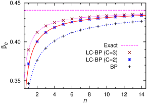
Figure 3: The inverse temperature $\beta_{c}$ at the ferromagnetic phase transition point of the square-lattice Ising model (no external field). The results obtained by the belief-propagation equation (BP, plus symbols) and those obtained by the loop-corrected belief-propagation equation (LC-BP) with memory capacity $C=2$ (star symbols) and memory capacity $C=3$ (cross symbols) are compared with the exact value $\beta_{c}\approx 0.4407$ (marked by the horizontal dashed line). Each square region of BP and LC-BP contains $n\times n$ vertices, with $n$ being the number of vertices along one boundary line of the square region. We can fit the data by the function $\beta_{c}=\beta_{c}^{\infty}-c\,n^{-\gamma}$, with $\beta_{c}^{\infty}=0.4490$, $c=0.1109$ and $\gamma=0.6075$ (for BP, bottom dashed curve), $\beta_{c}^{\infty}=0.4421$, $c=0.0746$ and $\gamma=0.8357$ (for LC-BP at $C=2$, middle solid curve), and $\beta_{c}^{\infty}=0.4417$, $c=0.0517$ and $\gamma=0.8071$ (for LC-BP at $C=3$, top dotted curve).

We need to modify Eq. (9) to remove this spurious self-field effect. Actually, if we strictly follow the Bethe-Peierls approximation, the expression for the probability distribution $q_{n\backslash m}(\sigma_{n})$ is not Eq. (9) but the following:

$$q_{n\backslash m}(\sigma_{n})=\frac{e^{\beta h^{0}_{n}\sigma_{n}}\prod\limits_{i\in\partial n\backslash m}\Bigl{[}\sum\limits_{\sigma_{i}}e^{\beta\sigma_{n}J_{ni}\sigma_{i}}q_{i\backslash\{m,n\}}(\sigma_{i})\Bigr{]}}{\sum\limits_{\sigma_{n}^{\prime}}e^{\beta h^{0}_{n}\sigma_{n}^{\prime}}\prod\limits_{i\in\partial n\backslash m}\Bigl{[}\sum\limits_{\sigma_{i}}e^{\beta\sigma_{n}^{\prime}J_{ni}\sigma_{i}}q_{i\backslash\{m,n\}}(\sigma_{i})\Bigr{]}}\;,$$ (10)

where $q_{i\backslash\{m,n\}}(\sigma_{i})$ is the marginal probability distribution of vertex $i$’s spin state in the cavity lattice $G_{\backslash\{m,n\}}$ with both vertex $m$ and $n$ being deleted (see Fig. 4).

In general, for any given vertex set $\phi$ and a vertex $n$ that is adjacent to at least one vertex in this set $\phi$, we denote by $q_{n\backslash\phi}(\sigma_{n})$ the marginal probability distribution of vertex $n$’s spin state in the cavity lattice $G_{\backslash\phi}$ obtained by deleting all the vertices of $\phi$ from the original lattice $G$. Under the Bethe-Peierls approximation, this probability distribution can be determined through

$$q_{n\backslash\phi}(\sigma)=\frac{e^{\beta h^{0}_{n}\sigma}\prod\limits_{i\in\partial n\backslash\phi}\Bigl{[}\sum\limits_{\sigma_{i}}e^{\beta\sigma J_{ni}\sigma_{i}}q_{i\backslash\{\phi,n\}}(\sigma_{i})\Bigr{]}}{\sum\limits_{\sigma_{n}}e^{\beta h^{0}_{n}\sigma_{n}}\prod\limits_{i\in\partial n\backslash\phi}\Bigl{[}\sum\limits_{\sigma_{i}}e^{\beta\sigma_{n}J_{ni}\sigma_{i}}q_{i\backslash\{\phi,n\}}(\sigma_{i})\Bigr{]}}\;,$$ (11)

where $\partial n\backslash\phi\equiv\partial n-\phi\cap\partial n$ denotes the vertex set obtained by deleting all the vertices of $\partial n$ that are also belonging to set $\phi$, and $\{\phi,n\}\equiv\phi\cup\{n\}$ is the vertex set obtained by adding vertex $n$ to set $\phi$.

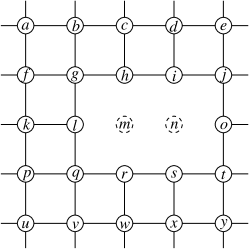
Figure 4: The cavity square lattice $G_{\backslash\{m,n\}}$ obtained by deleting vertices $m$ and $n$ (and all the attached edges) from the lattice $G$ of Fig. 1.

Equations (8), (10) and (11) form a hierarchical series of self-consistent equations and we refer them collectively as the loop-corrected belief-propagation equation. For practical applications we have to make a cutoff to this message-passing hierarchy, so that a closed set of equations can be obtained and can be iterated numerically.

In the remaining part of this paper we mainly consider the simplest nontrivial cutoff by requiring that the vertex set $\phi$ of the cavity probability distribution $q_{n\backslash\phi}$ of any vertex $n$ can contain at most two vertices (i.e., memory capacity $C=2$). Under this additional restriction, then for the two vertices $l$ and $r$ in Fig. 4 we have

$$q_{l\backslash\{m,n\}}(\sigma_{l}) \propto e^{\beta h^{0}_{l}\sigma_{l}}\bigl{[}\sum{{}_{\sigma_{g}}}e^{\beta\sigma_{l}J_{lg}\sigma_{g}}q_{g\backslash\{l,m\}}(\sigma_{g})\bigr{]}$$

$$\quad\quad\times\bigl{[}\sum{{}_{\sigma_{k}}}e^{\beta\sigma_{l}J_{lk}\sigma_{k}}q_{k\backslash\{l,m\}}(\sigma_{k})\bigr{]}$$

$$\quad\quad\times\bigl{[}\sum{{}_{\sigma_{q}}}e^{\beta\sigma_{l}J_{lq}\sigma_{q}}q_{q\backslash\{l,m\}}(\sigma_{q})\bigr{]}\;,$$ (12a)

$$q_{r\backslash\{m,n\}}(\sigma_{r}) \propto e^{\beta h^{0}_{r}\sigma_{r}}\bigl{[}\sum{{}_{\sigma_{q}}}e^{\beta\sigma_{r}J_{rq}\sigma_{q}}q_{q\backslash\{r,m\}}(\sigma_{q})\bigr{]}$$

$$\quad\quad\times\bigl{[}\sum{{}_{\sigma_{w}}}e^{\beta\sigma_{r}J_{rw}\sigma_{w}}q_{w\backslash\{r,m\}}(\sigma_{w})\bigr{]}$$

$$\quad\quad\times\bigl{[}\sum{{}_{\sigma_{s}}}e^{\beta\sigma_{r}J_{rs}\sigma_{s}}q_{s\backslash\{r,n\}}(\sigma_{s})\bigr{]}\;.$$ (12b)

We consider $q_{s\backslash\{r,n\}}(\sigma_{s})$ instead of $q_{s\backslash\{r,m\}}(\sigma_{s})$ in the last line of Eq. (12b) because vertex $n$ has stronger influence to vertex $s$ than vertex $m$. The probability distribution $q_{s\backslash\{r,n\}}(\sigma_{s})$ of Eq. (12b) can be computed through

$$q_{s\backslash\{n,r\}}(\sigma_{s}) \propto e^{\beta h^{0}_{s}\sigma_{s}}\bigl{[}\sum{{}_{\sigma_{t}}}e^{\beta\sigma_{s}J_{st}\sigma_{t}}q_{t\backslash\{s,n\}}(\sigma_{t})\bigr{]}$$ (13)

$$\times\bigl{[}\sum{{}_{\sigma_{x}}}e^{\beta\sigma_{s}J_{sx}\sigma_{x}}q_{x\backslash\{r,s\}}(\sigma_{x})\bigr{]}\;.$$

When we apply Eqs. (12) and (13) to the square-lattice Ising model, we obtain a critical inverse temperature $\beta_{c}\approx 0.3716$ for the ferromagnetic phase transition, which is considerably better than the prediction of the naive BP, see Fig. 3. This is an encouraging result. We can further improve the performance of the loop-corrected BP mean field theory by allowing the set $\phi$ of deleted vertices in Eq. (11) to contain three or even more vertices. For example if the memory capacity is set to $C=3$ the value of $\beta_{c}$ estimated for the ferromagnetic Ising model increases to $\beta_{c}\approx 0.3896$ (see Fig. 3).

The mean magnetization $\langle\sigma_{m}\rangle$ of vertex $m$ and the mean spin correlation $\langle\sigma_{m}\sigma_{n}\rangle$ between vertex $m$ and $n$ are estimated through the following equations:

$$\langle\sigma_{m}\rangle =\sum\limits_{\sigma_{m}}\sigma_{m}q_{m}(\sigma_{m})\;,$$ (14a)

$$\langle\sigma_{m}\sigma_{n}\rangle =\frac{\sum\limits_{\sigma_{m},\sigma_{n}}\sigma_{m}\sigma_{n}e^{\beta J_{mn}\sigma_{m}\sigma_{n}}q_{m\backslash n}(\sigma_{m})q_{n\backslash m}(\sigma_{n})}{\sum\limits_{\sigma_{m},\sigma_{n}}e^{\beta J_{mn}\sigma_{m}\sigma_{n}}q_{m\backslash n}(\sigma_{m})q_{n\backslash m}(\sigma_{n})}\;.$$ (14b)

The mean energy of the whole system is then

$$\langle E\rangle=-\sum\limits_{m=1}^{N}h_{m}^{0}\langle\sigma_{m}\rangle-\sum\limits_{(m,n)\in G}J_{mn}\langle\sigma_{m}\sigma_{n}\rangle\;.$$ (15)

$\langle E\rangle$ of course depends on the inverse temperature $\beta$, let us emphasize this dependence by $\langle E\rangle_{\beta}$. The free energy $F(\beta)$ of the system is related to the mean energy through $\langle E\rangle_{\beta}=\frac{{\rm d}(\beta F)}{{\rm d}\beta}$, namely

$$F(\beta)=\frac{1}{\beta}\int\limits_{0}^{\beta}\langle E\rangle_{\beta^{\prime}}{\rm d}\beta^{\prime}-\frac{1}{\beta}N\ln 2\;.$$ (16)

5 Loop-corrected belief propagation at the region graph level

In essence, the loop-corrected BP mean field theory of the preceding section tries to completely eliminate the effect of a deleted vertex $m$ to the cavity lattice $G_{\backslash m}$ through the BP hierarchy Eqs. (10) and (11). But the loop-corrected BP hierarchy is also based on the Bethe-Peierls approximation and it does not consider any of the short-range correlations that are discarded from this approximation (e.g., the correlations among the vertices $l$, $h$, $n$, and $m$ in the cavity graph $G_{\backslash m}$ of Fig. 2). To take into account more short-range correlations, we follow the work of Zhou and Wang Zhou-Wang-2012 and construct the loop-corrected BP equation at the coarse-grained region graph level.

In the example of the square lattice, we completely cover the vertices of the whole lattice by a set of square regions without any overlap between the regions. Each square region contains $n\times n$ vertices and all the interaction edges within these vertices, see Fig. 5. Two neighboring regions interact with each other through the $n$ edges in between, and they are therefore considered as being connected at the region level. The region graph $\mathcal{R}$ constructed in this way, with each vertex representing a local square domain of $n\times n$ vertices, has the same topology as the original square lattice $G$.

The loop-corrected BP hierarchy can then be obtained for this region graph $\mathcal{R}$. Consider the region $\gamma_{5}$ of Fig. 5 as an example. Let us define $q_{\gamma_{5}\backslash\gamma_{2}}(\sigma_{m},\sigma_{n})$ as the probability of vertex $m$ taking spin value $\sigma_{m}$ and vertex $n$ taking spin value $\sigma_{n}$ in the cavity region graph $\mathcal{R}_{\backslash\gamma_{2}}$ obtained by deleting region $\gamma_{2}$ from $\mathcal{R}$. Other joint probability distributions can be defined in a similar way, e.g., $q_{\gamma_{5}\backslash\{\gamma_{1},\gamma_{2}\}}(\sigma_{m},\sigma_{n})$ is the joint probability distribution of $\sigma_{m}$ and $\sigma_{n}$ in the cavity region graph $\mathcal{R}_{\backslash\{\gamma_{1},\gamma_{2}\}}$ (with regions $\gamma_{1}$ and $\gamma_{2}$ being deleted). If we restrict the set $\phi$ of deleted regions in memory to containing two regions at most (i.e., memory capacity $C=2$), we obtain that

$$q_{\gamma_{5}\backslash\gamma_{2}}(\sigma_{m},\sigma_{n})\propto\sum{{}_{\sigma_{r},\sigma_{s}}}e^{-\beta E_{\gamma_{5}}}$$

$$\quad\quad\times\bigl{[}\sum{{}_{\sigma_{l},\sigma_{q}}}e^{-\beta E_{\gamma_{4}\gamma_{5}}}q_{\gamma_{4}\backslash\{\gamma_{2},\gamma_{5}\}}(\sigma_{l},\sigma_{q})\bigr{]}$$

$$\quad\quad\times\bigl{[}\sum{{}_{\sigma_{w},\sigma_{x}}}e^{-\beta E_{\gamma_{8}\gamma_{5}}}q_{\gamma_{8}\backslash\{\gamma_{2},\gamma_{5}\}}(\sigma_{w},\sigma_{x})\bigr{]}$$

$$\quad\quad\times\bigl{[}\sum{{}_{\sigma_{t},\sigma_{o}}}e^{-\beta E_{\gamma_{6}\gamma_{5}}}q_{\gamma_{6}\backslash\{\gamma_{2},\gamma_{5}\}}(\sigma_{t},\sigma_{o})\bigr{]}\;,$$ (17a)

$$q_{\gamma_{5}\backslash\{\gamma_{1},\gamma_{2}\}}(\sigma_{m},\sigma_{n})\propto\sum{{}_{\sigma_{r},\sigma_{s}}}e^{-\beta E_{\gamma_{5}}}$$

$$\quad\quad\times\bigl{[}\sum{{}_{\sigma_{l},\sigma_{q}}}e^{-\beta E_{\gamma_{4}\gamma_{5}}}q_{\gamma_{4}\backslash\{\gamma_{1},\gamma_{5}\}}(\sigma_{l},\sigma_{q})\bigr{]}$$

$$\quad\quad\times\bigl{[}\sum{{}_{\sigma_{w},\sigma_{x}}}e^{-\beta E_{\gamma_{8}\gamma_{5}}}q_{\gamma_{8}\backslash\{\gamma_{2},\gamma_{5}\}}(\sigma_{w},\sigma_{x})\bigr{]}$$

$$\quad\quad\times\bigl{[}\sum{{}_{\sigma_{t},\sigma_{o}}}e^{-\beta E_{\gamma_{6}\gamma_{5}}}q_{\gamma_{6}\backslash\{\gamma_{2},\gamma_{5}\}}(\sigma_{t},\sigma_{o})\bigr{]}\;,$$ (17b)

$$q_{\gamma_{5}\backslash\{\gamma_{2},\gamma_{4}\}}(\sigma_{m},\sigma_{n})\propto\sum{{}_{\sigma_{r},\sigma_{s}}}e^{-\beta E_{\gamma_{5}}}$$

$$\quad\quad\times\bigl{[}\sum{{}_{\sigma_{w},\sigma_{x}}}e^{-\beta E_{\gamma_{8}\gamma_{5}}}q_{\gamma_{8}\backslash\{\gamma_{4},\gamma_{5}\}}(\sigma_{w},\sigma_{x})\bigr{]}$$

$$\quad\quad\times\bigl{[}\sum{{}_{\sigma_{t},\sigma_{o}}}e^{-\beta E_{\gamma_{6}\gamma_{5}}}q_{\gamma_{6}\backslash\{\gamma_{2},\gamma_{5}\}}(\sigma_{t},\sigma_{o})\bigr{]}\;.$$ (17c)

In the above expressions, the quantity $E_{\gamma}$ denotes the internal energy of a region $\gamma$, for example

$$E_{\gamma_{5}}(\sigma_{m},\sigma_{n},\sigma_{r},\sigma_{s})=-h^{0}_{m}\sigma_{m}-h^{0}_{n}\sigma_{n}-h^{0}_{r}\sigma_{r}-h^{0}_{s}\sigma_{s}$$

$$\quad-J_{mn}\sigma_{m}\sigma_{n}-J_{ns}\sigma_{n}\sigma_{s}-J_{rs}\sigma_{r}\sigma_{s}-J_{mr}\sigma_{m}\sigma_{r}\;,$$ (18)

and $E_{\gamma\gamma^{\prime}}$ is the interaction energy between region $\gamma$ and region $\gamma^{\prime}$, for example

$$E_{\gamma_{4}\gamma_{5}}(\sigma_{l},\sigma_{m},\sigma_{q},\sigma_{r})=-J_{lm}\sigma_{l}\sigma_{m}-J_{qr}\sigma_{q}\sigma_{r}\;.$$ (19)

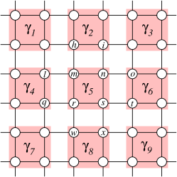
Figure 5: The square lattice coarse-grained as a region graph $\mathcal{R}$. Each square region ($\gamma_{1},\gamma_{2},\ldots$) contains $n\times n$ vertices and all the interactions within these vertices ($n=2$ in this particular example). Two nearest-neighboring regions interact through $n$ edges.

As Eq. (17) demonstrates, all the correlations within each region are precisely considered by summing over all the $2^{n^{2}}$ microscopic configurations of this region. In the practical implementation, the internal state summation is achieved through a numerical scheme that is efficient both in terms of computing time and in terms of needed memory (see Appendix A for details). By increasing the region size $n$ we can include more and more short-range correlations and achieve more precise quantitative predictions.

For the two-dimensional Ising model we have compared in Fig. 3 the results obtained by the conventional region-graph BP of Zhou-Wang-2012 and those obtained by the present region-graph loop-corrected BP. When the memory capacity is set to $C=2$ (the smallest nontrivial value), the iteration process of loop-corrected BP demands the same order of computational cost as that of BP, yet at each value of the square-region size $n$ the improvement of loop-corrected BP over BP is always significant, suggesting that loop-corrected BP is a much better choice than the naive BP for treating finite-dimensional lattice systems. Figure 6 compares the exact spontaneous magnetization of the square-lattice Ising model with the predictions obtained by BP and LC-BP ($C=2$). At each value of the region sizes used ($n=1$, $n=3$, or $n=5$) the improvement of LC-BP over BP is again significant.

It also appears that loop-corrected BP (with memory capacity $C=2$) outperforms the GBP method of Yedidia and coworkers Yedidia-Freeman-Weiss-2005 . When the square-region size is set to $n=2$, GBP predicts the critical inverse temperature of ferromagnetic phase transition to be $\beta_{c}\approx 0.4126$ Wang-Zhou-2013 ; a slightly better result is achieved by the loop-corrected BP method at square-region size $n^{\prime}=2n=4$, which reports a value of $\beta_{c}\approx 0.4186$. The GBP with square-region size $n=4$ predicts a value of $\beta_{c}\approx 0.429$ Wang-Zhou-2013 ; this result is marched by the loop-corrected BP at square-region size $n^{\prime}=2n=8$, which reports a value of $\beta_{c}\approx 0.4290$. We might therefore conjecture that GBP at square-region size $n$ and loop-corrected BP at square-region size $n^{\prime}=2n$ have comparable prediction power. Under such an assumption we can then argue that loop-corrected BP will be a better choice than GBP: (1) the iteration process of GBP is much more complicated than that of loop-corrected BP; and (2) the required computer storage space of a GBP message is of order $O(2^{n^{2}/2})$, making it unpractical to set the square-region size $n\geq 6$; (3) the required storage space of a loop-corrected BP message is only of order $O(2^{n})$, so we can set the square-region size to $n=20$ or even larger values. It should be pointed out that good performance of GBP can be achieved by increasing the size of the largest region one-dimensionally rather than two-dimensionally (see Kikuchi-Brush-1967 and Pelizzola-2005 ). It will be helpful to perform a comparative study by implementing LC-BP also in such a non-symmetric way. We leave this point for future investigations.

We can further improve the performance of the loop-corrected BP method by increasing the memory capacity $C$ (but at the cost of introducing many more cavity messages, see Appendix B). For the square-lattice Ising model, the results obtained by loop-corrected BP at $C=3$ are also shown in Fig. 3 to compare with the results obtained at $C=2$. We find that increasing $C$ from $C=2$ to $C=3$ does not bring a dramatic improvement to the prediction of $\beta_{c}$. Considering the high computation cost required for $C\geq 3$ (see Appendix B), if higher numerical precision is needed, it is more practical to increase the square-region size $n$ but to keep the memory capacity at $C=2$.

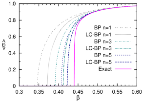
Figure 6: The spontaneous magnetization (the mean spin value $\langle\sigma\rangle$ of a vertex) of the square-lattice Ising model. The results obtained by belief propagation (BP) and those obtained by loop-corrected belief propagation (LC-BP) with memory capacity $C=2$ are shown together with the exact results (the solid line). Each square region of BP and LC-BP contains $n\times n$ vertices, with $n=1$, $3$, or $5$.

6 Conclusion

To summarize briefly, in this paper we described the main ideas of the loop-corrected belief propagation method and carried out an initial performance test on the square-lattice Ising model. The results in Fig. 3 and Fig. 6 clearly demonstrate that loop-corrected BP with memory capacity $C=2$ is much superior to the naive BP method, which is equivalent to loop-corrected BP with memory capacity $C=1$. The performance of loop-corrected BP further improves as the memory capacity is increased to $C=3$ or even larger values.

Our numerical results on the square-lattice Ising model also indicate that, compared to the generalized belief propagation method of Yedidia et al. Yedidia-Freeman-Weiss-2005 , the loop-corrected BP method (simply with memory capacity $C=2$) can achieve the same or even higher level of precision at much reduced computation cost. In addition, we wish to point out another very important advantage of the loop-corrected BP method: just as the survey propagation method is a natural extension of the naive BP method Mezard-Montanari-2009 ; ZhouBook , following the discussion of Zhou-Wang-2012 we might extend loop-corrected BP into the loop-corrected survey propagation method to study disordered lattice models in the low-temperature spin glass phase, where ergodicity of the configuration space is broken.

For the loop-corrected BP method really to be a helpful tool, it should be capable of giving good quantitative predictions on single instances of disordered lattice models. The performance of loop-corrected BP on the square-lattice and cubic-lattice spin glass models will be investigated and be reported in a forthcoming paper.

Appendix A: Message updating for a square region

To perform region-graph BP or loop-corrected BP iteration on a square lattce, the most demanding task is computing the joint probability distribution of spin states for the vertices on the boundary of a region. Let us consider the concrete example shown in Fig. 7. The central (C) square region contains $n\times n$ vertices with $n=6$, and it receives messages from three other square regions on the left (L), bottom (B), and right (R) side. Denote by $\underline{\sigma}_{T}\equiv(\sigma_{2},\sigma_{3},\ldots,\sigma_{7})$ a generic spin configuration for the $n$ vertices on the top (T) boundary of the central region. This spin configuration is affected by the interactions within the central region and the interactions between the central region and the three neighboring regions, and its probability distribution $P_{T}(\underline{\sigma}_{T})$ is expressed as

$$P_{T}(\underline{\sigma}_{T})\propto\sum\limits_{\underline{\sigma}_{C\backslash T}}e^{-\beta E_{C}}\Bigl{[}\sum\limits_{\underline{\sigma}_{L}}P_{L}(\underline{\sigma}_{L})e^{-\beta E_{L,C}}\Bigr{]}$$

$$\times\Bigl{[}\sum\limits_{\underline{\sigma}_{B}}P_{B}(\underline{\sigma}_{B})e^{-\beta E_{B,C}}\Bigr{]}\Bigl{[}\sum\limits_{\underline{\sigma}_{R}}P_{R}(\underline{\sigma}_{R})e^{-\beta E_{R,C}}\Bigr{]}\;.$$ (20)

In this expression, $\underline{\sigma}_{C\backslash T}\equiv(\sigma_{27},\sigma_{28},\ldots,\sigma_{55},\sigma_{56})$ is a spin configuration for all the other $(n-1)\times n$ vertices of the central region except the $n$ vertices at the top boundary, and $E_{C}$ is the total internal energy of this central region; $\underline{\sigma}_{L}\equiv(\sigma_{1},\sigma_{26},\ldots,\sigma_{22})$ is a spin configuration for the $n$ boundary vertices of the left region, and $P_{L}(\underline{\sigma}_{L})$ is an input probability distribution of $\underline{\sigma}_{L}$, and $E_{L,C}$ is the interation energy between the left and the central region; similarly, $\underline{\sigma}_{R}\equiv(\sigma_{13},\sigma_{12},\ldots,\sigma_{8})$ is a spin configuration for the boundary vertices of the right region, $P_{R}(\underline{\sigma}_{R})$ is an input probability distribution of $\underline{\sigma}_{R}$, $E_{R,C}$ is the interaction energy between the right and the central region, and $\underline{\sigma}_{B}\equiv(\sigma_{20},\sigma_{19},\ldots,\sigma_{15})$ is a spin configuration for the boundary vertices of the bottom region, $P_{B}(\underline{\sigma}_{B})$ is an input probability distribution of $\underline{\sigma}_{B}$, $E_{B,C}$ is the interaction energy between the bottom and the central region. Notice that the LC-BP equations (12), (13), and (17) all have the same form of Eq. (20).

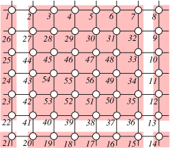
Figure 7: The central square region contains $n\times n$ vertices ($n=6$) and it interacts with the three neighboring square regions (partly shown) on the left, bottom, and right side.

According to Eq. (20), one needs to sum over a total number of $2^{n(n+2)}$ different spin configurations to determine the output probability $P_{T}(\underline{\sigma}_{T})$ of a single spin configuration $\underline{\sigma}_{T}$. A naive application of Eq. (20) is therefore feasible only for very small values of $n$ (e.g., $n\leq 3$).

We now introduce a numerical trick that greatly accelerate this summation process. By this simple trick we reduce the total number of needed operations to sum over all the spin configurations from $O(2^{n(n+2)})$ to $O(n^{2}2^{n})$, and also dramatically reduce the total amount of storage space needed in the numerical computation.

First we notice that, due to the binary nature of the spins, a generic probability distribution $p(\sigma_{1},\sigma_{2},\ldots,\sigma_{n})$ over $n$ spins can be written in the following form:

$$p(\sigma_{1},\ldots,\sigma_{n})=\sum\limits_{s_{1}=0}^{1}\sum\limits_{s_{2}=0}^{1}\ldots\sum\limits_{s_{n}=0}^{1}c_{s_{1}s_{2}\ldots s_{n}}\sigma_{1}^{s_{1}}\sigma_{2}^{s_{2}}\ldots\sigma_{n}^{s_{n}}\;,$$ (21)

where $s_{i}\in\{0,1\}$ for $i=1,2,\ldots,n$ and $\{c_{s_{1}s_{2}\ldots s_{n}}\}$ is a set of $2^{n}$ coefficients, with $c_{00\ldots 0}\equiv 2^{-n}$ due to the normalization constraint. Therefore the probability distribution $p(\sigma_{1},\sigma_{2},\ldots,\sigma_{n})$ is completely characterized by the coefficient set $\{c_{s_{1}s_{2}\ldots s_{n}}\}$.

Due to the fact that

$$e^{\beta h_{i}\sigma_{i}} \equiv\cosh(\beta h_{i})\bigl{[}1+\tanh(\beta h_{i})\sigma_{i}\bigr{]}\;,$$ (22a)

$$e^{\beta J_{ii^{\prime}}\sigma_{i}\sigma_{i^{\prime}}} \equiv\cosh(\beta J_{ii^{\prime}})\bigl{[}1+\tanh(\beta J_{ii^{\prime}})\sigma_{i}\sigma_{i^{\prime}}\bigr{]}\;,$$ (22b)

then for $i,j\in\{1,2,\ldots,n\}$ ($i<j$) and $i^{\prime}\notin\{1,2,\ldots,n\}$,

$$e^{\beta h_{i}\sigma_{i}}p(\sigma_{1},\ldots,\sigma_{n})=\cosh(\beta h_{i})\sum\limits_{s_{1}s_{2}\ldots s_{n}}\sigma_{1}^{s_{1}}\sigma_{2}^{s_{2}}\ldots s_{n}^{s_{n}}$$

$$\quad\times\bigl{[}c_{s_{1}s_{2}\ldots s_{n}}+\tanh(\beta h_{i})c_{s_{1}\ldots s_{i-1}\overline{s}_{i}s_{i+1}\ldots s_{n}}\bigr{]}\;,$$ (23a)

$$\sum{{}_{\sigma_{i}}}e^{\beta J_{ii^{\prime}}\sigma_{i}\sigma_{i^{\prime}}}p(\sigma_{1},\ldots,\sigma_{n})=2\cosh(\beta J_{ii^{\prime}})$$

$$\quad\times\sum\limits_{s_{1}s_{2}\ldots s_{n}}\sigma_{1}^{s_{1}}\ldots\sigma_{i-1}^{s_{i-1}}\sigma_{i^{\prime}}^{s_{i}}\sigma_{i+1}^{s_{i+1}}\ldots s_{n}^{s_{n}}$$

$$\quad\quad\times\bigl{[}(1-s_{i}+s_{i}\tanh(\beta J_{ii^{\prime}})\bigr{]}c_{s_{1}s_{2}\ldots s_{n}}\;,$$ (23b)

$$e^{\beta J_{ij}\sigma_{i}\sigma_{j}}p(\sigma_{1},\ldots,\sigma_{n})=\cosh(\beta J_{ij})\times$$

$$\quad\sum\limits_{s_{1}s_{2}\ldots s_{n}}\sigma_{1}^{s_{1}}\sigma_{2}^{s_{2}}\ldots s_{n}^{s_{n}}\bigl{[}c_{s_{1}s_{2}\ldots s_{n}}+$$

$$\quad\quad\quad\tanh(\beta J_{ij})c_{s_{1}\ldots s_{i-1}\overline{s}_{i}s_{i+1}\ldots s_{j-1}\overline{s}_{j}s_{j+1}\ldots s_{n}}\bigr{]}\;,$$ (23c)

where $\overline{s}_{i}=1$ if $s_{i}=0$ and $\overline{s}_{i}=0$ if $s_{i}=1$. Equation (23) therefore gives a set of rules on how the coefficients set $\{c_{s_{1}s_{2}\ldots s_{n}}\}$ changes as $p(\sigma_{1},\ldots,\sigma_{n})$ is perturbed by multiplication and summation.

We simplify the computation of Eq. (20) by treating the three input probability distributions separately. For example, starting from the input probability distribution $P_{B}(\sigma_{20},\sigma_{19},\ldots,\sigma_{15})$ of the bottom region (see Fig. 8), we obtain a probability distribution $Q_{B}(\sigma_{41},\sigma_{53},\ldots,\sigma_{36})$ for the set of $n$ boundary vertices $\{41,53,55,56,50,36\}$ through the following recursive process: (1) initialize the coefficients set of $Q_{B}(\cdot)$ to be identical to that of $P_{B}(\cdot)$; (2) then consider sequentially all the $n$ vertical edges $\langle 20,41\rangle$, $\langle 19,40\rangle$, …, $\langle 15,36\rangle$ between the central and the bottom region and modify the coefficients set of $Q_{B}(\cdot)$ according to Eq. (23b); (3) then consider sequentially all the $(n-1)$ horizontal edges $\langle 41,40\rangle$, $\langle 40,39\rangle$, …, $\langle 37,36\rangle$ between the set of vertices $\{41,40,39,38,37,36\}$ and further modify the coefficients set of $Q_{B}(\cdot)$ according to Eq. (23c); (4) then consider sequentially all the $(n-1)$ external fields on the set of internal vertices $\{40,39,\ldots,37\}$ and further modify the coefficients set of $Q_{B}(\cdot)$ according to Eq. (23a); (5) repeat the previous three steps on the row containing the set of vertices $\{53,52,51,50\}$: apply Eq. (23b) on the set of vertical edges $\{\langle 40,53\rangle,\ldots,\langle 37,50\rangle\}$ and then apply Eq. (23c) on the horizontal edges $\langle 53,52\rangle$, $\langle 52,51\rangle$ and $\langle 51,50\rangle\}$, and then apply Eq. (23a) on the internal vertices $52$ and $51$; (6) finally, apply Eq. (23b) on the edges $\langle 52,55\rangle$ and $\langle 51,56\rangle$, and apply Eq. (23c) on edge $\langle 55,56\rangle$ and then output the coefficients set of $Q_{B}(\sigma_{41},\sigma_{53},\sigma_{55},\sigma_{56},\sigma_{50},\sigma_{36})$.

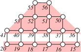
Figure 8: Given an input probability distribution $P_{B}(\sigma_{20},\ldots,\sigma_{15})$ for the set $\{20,19,\ldots,15\}$ of vertices on the bottom row, the probability distribution $Q_{B}(\sigma_{41},\ldots,\sigma_{36})$ for the set $\{41,53,55,56,50,36\}$ of boundary vertices can be determined by recursion from the bottom row up to the top row.

The joint probability distributions $Q_{L}(\sigma_{2},\ldots,\sigma_{41})$ for the set of vertices $\{2,28,46,55,53,41\}$ and $Q_{R}(\sigma_{36},\ldots,\sigma_{7})$ for the set of vertices $\{36,50,56,47,31,7\}$, see Fig. 7, are obtained through the same recursive process starting from $P_{L}(\cdot)$ and $P_{R}(\cdot)$, respectively. The only additional feature is that we now need to consider the external fields of all the vertices in these two boundary sets (again through applying Eq. (23a) to $Q_{L}(\cdot)$ and $Q_{R}(\cdot)$ repeatedly).

With these preparations, we then obtain a joint probability distribution $Q(\sigma_{2},\ldots,\sigma_{7})$ for the set of vertices $\{2,28,46,47,31,7\}$ through the following expression:

$$Q(\sigma_{2},\sigma_{28},\sigma_{46},\sigma_{47},\sigma_{31},\sigma_{7})\propto e^{\beta J_{46,47}\sigma_{46}\sigma_{47}}\times$$

$$\sum\limits_{\sigma_{41},\sigma_{53},\sigma_{55}}\sum\limits_{\sigma_{56},\sigma_{50},\sigma_{36}}Q_{L}(\sigma_{2},\sigma_{28},\sigma_{46},\sigma_{55},\sigma_{53},\sigma_{41})$$

$$\quad\quad\times Q_{B}(\sigma_{41},\sigma_{53},\sigma_{55},\sigma_{56},\sigma_{50},\sigma_{36})$$

$$\quad\quad\times Q_{R}(\sigma_{36},\sigma_{50},\sigma_{56},\sigma_{47},\sigma_{31},\sigma_{7})$$

$$\propto e^{\beta J_{46,47}\sigma_{46}\sigma_{47}}\sum\limits_{s_{2}s_{28}s_{46}s_{47}s_{31}s_{7}}\sigma_{2}^{s_{2}}\sigma_{28}^{s_{28}}\sigma_{46}^{s_{46}}\sigma_{47}^{s_{47}}\sigma_{31}^{s_{31}}\sigma_{7}^{s_{7}}$$

$$\quad\quad\times\sum\limits_{s_{55}s_{53}s_{41}}\sum\limits_{s_{36}s_{50}s_{56}}c_{s_{2}s_{28}s_{46}s_{55}s_{53}s_{41}}^{(L)}$$

$$\quad\quad\quad\quad\times c_{s_{41}s_{53}s_{55}s_{56}s_{50}s_{36}}^{(B)}c_{s_{36}s_{50}s_{56}s_{47}s_{31}s_{7}}^{(R)}\;.$$ (24)

In the above expression, the coefficient sets $\{c_{s_{2}\cdots s_{41}}^{(L)}\}$, $\{c_{s_{41}\cdots s_{36}}^{(B)}\}$, and $\{c_{s_{36}\cdots s_{7}}^{(R)}\}$ correspond to $Q_{L}(\cdot)$, $Q_{B}(\cdot)$, and $Q_{R}(\cdot)$, respectively. The effect of the multiplication term $e^{\beta J_{46,47}\sigma_{46}\sigma_{47}}$ to the coefficient set of the probability distribution $Q(\cdot)$ can again be obtained through Eq. (23c).

Finally, the probability distribution $P_{T}(\sigma_{2},\ldots,\sigma_{7})$ for the set $\{2,3,4,5,6,7\}$ of vertices at the top boundary is determined from $Q(\sigma_{2},\sigma_{28},\sigma_{46},\sigma_{47},\sigma_{31},\sigma_{7})$ through the following recursive process (see Fig. 9): (1) set the coefficients set of $P_{T}(\cdot)$ to be identical to that of $Q(\cdot)$; (2) then consider the vertical edges $\langle 29,46\rangle$ and $\langle 30,47\rangle$ sequentially and modify the coefficients set of $P_{T}(\cdot)$ according to Eq. (23b); (3) then consider all the horizontal edges $\langle 28,29\rangle$, $\langle 29,30\rangle$, and $\langle 30,31\rangle$ between the set of vertices $\{28,29,30,31\}$ and the external fields on vertices $29$ and $30$ and further modify the coefficients set of $P_{T}(\cdot)$ according to Eq. (23c) and Eq. (23a), respectively; (4) repeat the operations of steps (2) and (3) on the vertical edges between the top and the second row of Fig. 9, the horizontal edges of the top row, and the set of vertices $\{3,4,5,6\}$. We then output the resulting coefficient set of $P_{T}(\cdot)$ as the result of original computing task Eq. (20).

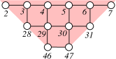
Figure 9: Given an input joint probability distribution $Q(\sigma_{2},\ldots,\sigma_{7})$ for the set $\{2,28,46,47,31,7\}$ of vertices on the bottom boundary, the joint probability distribution $P_{T}(\sigma_{2},\ldots,\sigma_{7})$ for the set $\{2,3,4,5,6,7\}$ on the top row can be determined recursively from the bottom row up to the top row.

It is straightforward to extend the numerical trick of this appendix to other values of even $n$ and also to the cases of $n$ being odd. For studying lattice models on a three-dimensional cubic lattice, this same trick can be applied to a cubic region containing $n\times n\times n$ vertices.

Appendix B: Loop-corrected belief propagation with memory capacity $C=3$

When the memory capacity is set to $C=3$, then with respective to a focal vertex or region (denoted by a filled small square in each block of Fig. 10), we need to consider $29$ different patterns of the three deleted vertices or regions (denoted by three unfilled small squares in each block of Fig. 10). These $29$ patterns are indexed as $00$, $01a$ and $01b$, $02a$ and $02b$, $\ldots$, $13a$ and $13b$, $14$, and $15$ in Fig. 10 for the convenience of discussion. The patterns $01a$ and $01b$ (and similarly $02a$ and $02b$, $03a$ and $03b$, …) are related by a mirror symmetry.

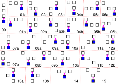
Figure 10: When the memory capacity is set to $C=3$, each focal vertex/region (denoted by a filled small square) needs to remember the positions of the other three deleted vertices/regions (denoted by three unfilled small squares). In total we need to distinguish $29$ different patterns of the three deleted vertices/regions, which are indexed as $00$, $01a$ and $01b$, $\ldots$, $14$, and $15$. The small arrows indicate the cavity message of the focal vertex/region to the deleted vertices/regions. For the purpose of clarity we separate different patterns through the thin dashed lines.

Each pattern of Fig. 10 is associated with a cavity message. For example, suppose vertices $l$, $m$, $n$ are deleted from the graph $G$ of Fig. 1, then the pattern $01a$ of Fig. 10 corresponds to the cavity message $q_{s\backslash\{l,m,n\}}(\sigma_{s})$ from vertex $s$ to vertex $n$, while pattern $01b$ corresponds to the cavity message $q_{q\backslash\{l,m,n\}}(\sigma_{q})$ from vertex $q$ to vertex $l$. As another example at the region graph level, suppose regions $\gamma_{2}$, $\gamma_{6}$ and $\gamma_{9}$ are deleted from the region graph $\mathcal{R}$ of Fig. 5, then the pattern $03b$ of Fig. 10 corresponds to the cavity message $q_{\gamma_{5}\backslash\{\gamma_{2},\gamma_{6},\gamma_{9}\}}(\sigma_{m},\sigma_{n})$ from region $\gamma_{5}$ to $\gamma_{2}$.

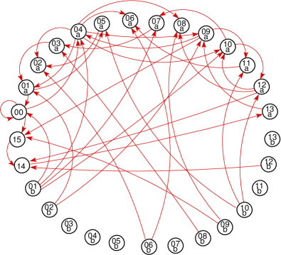
Figure 11: Diagram showing how the cavity message of all the $29$ patterns in Fig. 10 are iteratively determined (see main text for more details). For reason of clarity, for each pair of mirror patterns (say $01a$ and $01b$) we only draw the input edges to one of the patterns ($01a$) but not to the mirror pattern ($01b$). The edges to each mirror pattern can be easily constructed by symmetry considerations. For example, since pattern $01a$ receives edges from patterns $02b$, $03a$ and $04a$, then pattern $01b$ must receive edges from patterns $02a$, $03b$ and $04b$.

The iteration of the $29$ cavity messages for the $29$ patterns of Fig. 10 is carried out following the updating diagram of Fig. 11. Each directed edge $p_{1}\rightarrow p_{2}$ in this diagram points from one pattern (say $p_{1}=04a$) to another pattern (say $p_{2}=01a$), and it means that the cavity message of pattern $p_{2}$ is determined (partly) from the cavity message of pattern $p_{1}$. For example, there are three directed edges (from patterns $01a$, $01b$ and $00$, respectively) to pattern $00$, meaning that the output cavity message of pattern $00$ can be computed based on three inputing cavity messages from patterns $00$, $01a$ and $01b$. In the specific case of Fig. 1, we have

$$q_{r\backslash\{c,h,m\}}(\sigma_{r})\propto e^{\beta h^{0}_{r}\sigma_{r}}\bigl{[}\sum{{}_{\sigma_{q}}}e^{\beta J_{qr}\sigma_{q}\sigma_{r}}q_{q\backslash\{h,m,r\}}(\sigma_{q})\bigr{]}$$

$$\quad\quad\quad\quad\times\bigl{[}\sum{{}_{\sigma_{w}}}e^{\beta J_{wr}\sigma_{w}\sigma_{r}}q_{w\backslash\{h,m,r\}}(\sigma_{w})\bigr{]}$$

$$\quad\quad\quad\quad\times\bigl{[}\sum{{}_{\sigma_{s}}}e^{\beta J_{sr}\sigma_{s}\sigma_{r}}q_{s\backslash\{h,m,r\}}(\sigma_{s})\bigr{]}\;.$$ (25)

The updating equations for the other $28$ cavity messages can be written down in a similar way according to Fig. 11. Notice that in Fig. 11 we only draw the input edges to patterns $00$, $14$, $15$ and patterns $01a$, $02a$, $\ldots$, $13a$ but not the input edges to all the mirror patterns $01b$, $02b$, $\ldots$, $13b$ to avoid the diagram being too complicated. We can easily construct all the missing directed edges by symmetry considerations. For example, since pattern $03a$ receives edges from patterns $07a$ and $08b$, then pattern $03b$ must receive edges from patterns $07b$ and $08a$. In the specific case of regions $\gamma_{2}$, $\gamma_{6}$, and $\gamma_{9}$ being deleted from Fig. 5, we have

$$q_{\gamma_{5}\backslash\{\gamma_{2},\gamma_{6},\gamma_{9}\}}(\sigma_{m},\sigma_{n})\propto e^{\beta h^{0}_{m}\sigma_{m}+\beta h^{0}_{n}\sigma_{n}+\beta J_{mn}\sigma_{m}\sigma_{n}}$$

$$\quad\times\sum\limits_{\sigma_{r},\sigma_{s}}\bigl{[}\sum\limits_{\sigma_{l},\sigma_{q}}e^{\beta J_{lm}\sigma_{l}\sigma_{m}+\beta J_{qr}\sigma_{q}\sigma_{r}}q_{\gamma_{4}\backslash\{\gamma_{2},\gamma_{5},\gamma_{9}\}}(\sigma_{l},\sigma_{q})\bigr{]}$$

$$\quad\quad\quad\times\bigl{[}\sum\limits_{\sigma_{w},\sigma_{x}}e^{\beta J_{wr}\sigma_{w}\sigma_{r}+\beta J_{xs}\sigma_{x}\sigma_{s}}q_{\gamma_{8}\backslash\{\gamma_{2},\gamma_{5},\gamma_{9}\}}(\sigma_{w},\sigma_{x})\bigr{]}\;.$$

References

- (1) J. Pearl, Probabilistic Reasoning in Intelligent Systems: Networks of Plausible Inference (Morgan Kaufmann, San Franciso, CA, USA, 1988)
- (2) M. Mézard, G. Parisi, M. A. Virasoro, Spin Glass Theory and Beyond (World Scientific, Singapore, 1987)
- (3) H. A. Bethe, Statistical theory of superlattices. Proc. R. Soc. London A 150, 552–575 (1935)
- (4) R. Peierls, On Ising’s model of ferromagnetism. Proc. Camb. Phil. Soc. 32, 477–481 (1936)
- (5) T. S. Chang, An extension of Bethe’s theory of order-disorder transitions in metallic alloys. Proc. R. Soc. London A 161, 546–563 (1937)
- (6) M. Mézard, A. Montanari, Information, Physics, and Computation (Oxford Univ. Press, New York, 2009)
- (7) J. S. Yedidia, W. T. Freeman, Y. Weiss, Constructing free-energy approximations and generalized belief-propagation algorithms. IEEE Trans. Inf. Theory 51, 2282–2312 (2005)
- (8) A. Pelizzola, Cluster variation method in statistical physics and probabilistic graphical models. J. Phys. A: Meth. Gen. 38, R309–R339 (2005)
- (9) T. Rizzo, A. Lage-Castellanos, R. Mulet, F. Ricci-Tersenghi, Replica cluster variational method. J. Stat. Phys. 139, 375–416 (2010)
- (10) C. Wang, H.-J. Zhou, Simplifying generalized belief propagation on redundant region graphs. J. Phys.: Conf. Series 473, 012004 (2013)
- (11) A. Lage-Castellanos, R. Mulet, F. Ricci-Tersenghi, Message passing and Monte Carlo algorithms: connecting fixed points with metastable states. Europhys. Lett. 107, 57011 (2014)
- (12) R. Kikuchi, A theory of cooperative phenomena. Phys. Rev. 81, 988–1003 (1951)
- (13) G. An, A note on the cluster variation method. J. Stat. Phys. 52, 727–734 (1988)
- (14) H.-J. Zhou, C. Wang, Region graph partition function expansion and approximate free energy landscapes: Theory and some numerical results. J. Stat. Phys. 148, 513–547 (2012)
- (15) S. F. Edwards, P. W. Anderson, Theory of spin glasses. J. Phys. F: Met. Phys. 5, 965–974 (1975)
- (16) H. Nishimori, Statistical Physics of Spin Glasses and Information Processing: An Introduction (Clarendon Press, Oxford, 2001)
- (17) A. Montanari, T. Rizzo, How to compute loop corrections to Bethe approximation. J. Stat. Mech.: Theo. Exp. P10011 (2005)
- (18) G. Parisi, F. Slanina, Loop expansion around the Bethe-Peierls approximation for lattice models. J. Stat. Mech.: Theo. Exp. L02003 (2006)
- (19) M. Chertkov, V. Y. Chernyak, Loop series for discrete statistical models on graphs. J. Stat. Mech.: Theor. Exp. P06009 (2006)
- (20) J. Mooij, B. Wemmenhove, B. Kappen, T. Rizzo, Loop corrected belief propagation. J. Machine Learning Res.: Workshop Conf. Proc. 2, 331–338 (2007)
- (21) Y. Bulatov, Cycle-corrected belief propagation. preprint: www.yaroslavvb.com/papers/bulatov-cycle.pdf (2008)
- (22) J.-Q. Xiao, H.-J. Zhou, Partition function loop series for a general graphical model: free-energy corrections and message-passing equations. J. Phys. A: Math. Theor. 44, 425001 (2011)
- (23) S. Ravanbakhsh, C.-N. Yu, R. Greiner, A generalized loop correction method for approximate inference in graphical models. In Proc. 29th Int. Conf. Machine Learning (ICML-12), 543–550 (Edinburgh, Scotland, UK, 2012)
- (24) D. Weitz, Counting independent sets up to the tree threshold. In Proceedings of the Thirty-Eighth Annual ACM Symposium on Theory of Computing (STOC ’06), 140–149 (ACM, New York, NY, USA, 2006)
- (25) E. Ising, Beitrag zur theorie des ferromagnetismus. Zeit. Physik 31, 253–258 (1925)
- (26) K. Huang, Statistical Mechanics (John Wiley, New York, 1987), 2nd edn
- (27) H.-J. Zhou, Spin Glass and Message Passing (in Chinese) (Science Press, Beijing, 2015)
- (28) H. A. Kramers, G. H. Wannier, Statistics of the two-dimensional ferromagnet. Part I. Phys. Rev. 60, 252–262 (1941)
- (29) H. A. Kramers, G. H. Wannier, Statistics of the two-dimensional ferromagnet. Part II. Phys. Rev. 60, 263–276 (1941)
- (30) A. Lage-Castellananos, R. Mulet, F. Ricci-Tersenghi, T. Rizzo, Inference algorithm for finite-dimensional spin glasses: Belief propagation on the dual lattice. Phys. Rev. E 84, 046706 (2011)
- (31) I. Morgenstern, K. Binder, Magnetic correlations in two-dimensional spin-glasses. Phys. Rev. B 22, 288–303 (1980)
- (32) L. Saul, M. Kardar, Exact integer algorithm for the two-dimensional Ising spin glass. Phys. Rev. E 48, R3221–R3224 (1993)
- (33) J. Houdayer, A cluster monte carlo algorithm for 2-dimensional spin glasses. Eur. Phys. J. B 22, 479–484 (2001)
- (34) T. Jörg, J. Lukic, E. Marinari, O. C. Martin, Strong universality and algebraic scaling in two-dimensional Ising spin glasses. Phys. Rev. Lett. 96, 237205 (2006)
- (35) C. K. Thomas, A. A. Middleton, Exact algorithm for sampling the two-dimensional Ising spin glass. Phys. Rev. E 80, 046708 (2009)
- (36) F. P. Toldin, A. Pelissetto, E. Vicari, Universality of the glassy transitions in the two-dimensional Ising model. Phys. Rev. E 82, 021106 (2010)
- (37) C. K. Thomas, D. A. Huse, A. A. Middleton, Zero- and low-temperature behavior of the two-dimensional Ising spin glass. Phys. Rev. Lett. 107, 047203 (2011)
- (38) F. P. Toldin, A. Pelissetto, E. Vicari, Finite-size scaling in two-dimensional Ising spin-glass models. Phys. Rev. E 84, 051116 (2011)
- (39) R. Kikuchi, S. G. Brush, Improvement of the cluster-variation method. J. Chem. Phys. 47, 195–203 (1967)