Measuring and using non-markovianity

Abstract

We construct measures for the non-Markovianity of quantum evolution with a physically meaningful interpretation. We first provide a general setting in the framework of channel capacities and propose two families of meaningful quantitative measures, based on the largest revival of a channel capacity, avoiding some drawbacks of other non-Markovianity measures. We relate the proposed measures to the task of information screening. This shows that the non-Markovianity of a quantum process may be used as a resource. Under these considerations, we analyze two paradigmatic examples, a qubit in a quantum environment with classically mixed dynamics and the Jaynes-Cummings model.

I Introduction

The field of open quantum systems is of paramount importance in quantum theory Breuer and Petruccione (2007). It helps to understand fundamental problems as decoherence, the quantum to classical transition, or the measurement problem Schlosshauer (2007). Besides, it has been essential to reach an impressive level of control in experiments of different quantum systems, which are the cornerstone in recent development of quantum technologies Raimond et al. (2001); Leibfried et al. (2003); Bloch et al. (2008); Furusawa and Vuckovic (2009); Ladd et al. (2010).

The usual approach to quantum open systems relies on the assumption that the evolution has negligible memory effects. This supposition is part of the so-called Born-Markov approximation, which also assumes weak system-environment coupling and a large environment. The keystone of Markovian quantum dynamics is the Lindblad master equation Lindblad (1976); Gorini et al. (1976) which describes the generator of quantum dynamical semigroups. The behavior of several interesting and realistic quantum systems has been studied using the Born-Markov approximation. However, these assumptions (weak coupling or large size of the environment) cannot be applied in many situations, including recent experiments of quantum control. This shows the importance of understanding quantum open systems beyond the Born-Markov approximation.

A great amount of work (see Breuer (2012); Rivas et al. (2014) and references therein) has been done to understand and characterize non-Markovian quantum evolutions or non-Markovianity (NM) – as it is generically called. This not only gives us a better understanding of open quantum systems but also provides more efficient ways to control quantum systems. For example, it was recently shown that non-Markovianity is an essential resource in some instances of steady state entanglement preparation Huelga et al. (2012); Cormick et al. (2013) or can be exploited to carry out quantum control tasks that could not be realized in closed systems Reich et al. . Besides, non-Markovian environments can speed up quantum evolutions reducing the quantum speed limit Deffner and Lutz (2013).

Unlike other properties, like entanglement, there is not a unique definition of non-Markovianity. There exist different criteria, more or less physically motivated, which in turn can be associated to a measure Breuer (2012); Rivas et al. (2014). The two most popular criteria are based on distinguishability Breuer et al. (2009) and divisibility Rivas et al. (2010), from which two corresponding measures can be derived. There exist other measures Lu et al. (2010); Vasile et al. (2011); Luo et al. (2012); Lorenzo et al. (2013); Bylicka et al. (2014) which are basically variations of these two or are very similar. All of these measures present some of the following problems: Lack of a clear and intuitive physical interpretation, they can diverge in very generic cases Žnidarič et al. (2011), and they are not directly comparable between them. Another problem is that, even if at least one of them has an intuitive physical interpretation, in terms of information flow Breuer et al. (2009), neither, to our knowledge, has a direct relation to a resource associated to a task – like entanglement of formation has.

In this work, we pursue two goals. First, we want to construct NM measures without the mentioned drawbacks. We undertake this task within the framework of channel capacities. The proposed measures are based on the maximum revival of the capacities, a characteristic that has a very simple physical interpretation and has a natural time-independent bound. Of course there might – and most likely will – exist many possible measures of quantum non- Markovianity. Thus, we first provide a general setting and then put forward two plausible, meaningful quantitative measures. Our second goal is to outline the theoretical bases for considering NM as a resource.

Consider what we call a quantum vault (QV). Alice shall deposit information, classical or quantum, in a quantum physical system (say in a physical realization of a qubit); during some time, through which the system evolves, the physical system can be subject to an attack by an eavesdropper, Eve; finally, after that time interval, the information is to be retrieved by Alice from the same physical system. Of course, the system interacts with an environment, to which neither Alice nor Eve can access. Notice that this task can be related with quantum data hiding Divincenzo et al. (2002); DiVincenzo et al. (2003); Matthews et al. (2009). We show that one of the NM measures proposed is closely related to the efficiency of the quantum vault. Therefore the value of the measure can be considered a resource associated to a specific task.

To illustrate our ideas we analyze two examples of physical systems coupled to non-Markovian environments, and analyze the newly defined measures as well as their quantum vault capabilities. We also explain possible advantages with respect to other NM measures. First we study a qubit, coupled via pure dephasing to an environment whose dynamics are given by a mixed quantum map. Different kinds of dynamics can be explored, changing the initial state of the environment. For the measures proposed in previous works, this sometimes leads to an unexpected behavior. The other example we consider is the well known Jaynes-Cummings model (JCM) Jaynes and Cummings (1963), a two level atom coupled to a bosonic bath, where we contrast our proposals, with some of the most used NM measures.

The work is organized as follows. In Sec. II we describe the general framework that relates NM with capacities of a quantum channel. Then, we define two NM measures based on the largest revival of the capacities. In Sec. III we introduce the concept of quantum vault and show its relation to the new NM measures. Sec. IV is devoted to analyzing two examples using the ideas presented in the previous sections. We end the paper with some final remarks in Sec. V.

II Non-Markovianity measured by the largest revival

The two most widely spread NM measures are, one due to Breuer et al. Breuer et al. (2009) based on distinguishability (in the following abbreviated by “BLP”), and the other due to Rivas et al. Rivas et al. (2010) based on divisibility (“RHP”). At the heart of both measures, there is a well defined concept which has been borrowed from classical stochastic systems. In the case of BLP, it is the contraction of probability space under Markovian stochastic processes, while in the case of RHP, it is the divisibility of the process itself. Both concepts can be used as criteria for quantum Markovianity by defining that a quantum process is Markovian if the distinguishability between all pairs of evolving states is non-increasing (BLP-property), or if the process is divisible (RHP-property); otherwise the process is called non-Markovian. It has been shown in Ref. Rivas et al. (2014), that the semigroup property of a quantum process implies the RHP-property and that the RHP-property implies the BLP-property. In order to obtain a non-Markovianity (NM) measure, both groups of authors apply essentially the same procedure: integrate a differential measure for the violation of the corresponding criterion. The same construction principle has been used in Ref. Bylicka et al. (2014), to quantify NM based on channel capacities.

Consider the convex space of all quantum channels, and in this space a continuous curve $\Lambda_{t}$ with $0\leq t\leq\infty$ starting at the identity $\Lambda_{0}=\openone$. We will call such a curve a quantum process. Any resource $\mathcal{K}$ of interest will be a function on the space of quantum channels. Thus any quantum process comes along with the function

$$K(t)=\mathcal{K}(\Lambda_{t}),$$ (1)

quantifying the resource the quantum channel provides at time $t$. Postulating that $K(t)$ cannot increase during Markovian dynamics, one defines the function

$$\mathcal{M}^{\infty}_{\mathcal{K}}[\Lambda_{t}]=\int_{\dot{K}>0}\dot{K}(\tau)\,\mathrm{d}\tau\;,$$ (2)

as a measure for non-Markovianity. We use the subscript $\infty$ for this class of measures, as it is possible that one has to add an infinite number of contributions (all intervals where $\dot{K}$ ¿ 0). We use brackets to indicate a functional on the space of quantum processes, and parenthesis when we refer to a functional on the space of quantum channels. One can immediately derive a criterion for non-Markovianity, namely $\mathcal{M}^{\infty}_{\mathcal{K}}[\Lambda_{t}]>0$. In the case of RHP,

$$\dot{K}(\tau)=\lim_{\varepsilon\to 0^{+}}\frac{{\rm tr}|C_{\tau+\varepsilon,\tau}|-1}{\varepsilon}\;,$$ (3)

where ${\rm tr}|\hat{A}|$ is the trace-norm and $C_{\tau+\varepsilon,\tau}$ is the Choi representation Bengtsson and Zyczkowski (2006); Heinosaari and Ziman (2012) of the map $\Lambda_{\tau+\varepsilon}\circ\Lambda_{\tau}^{-1}$, which evolves states from time $\tau$ to time $\tau+\varepsilon$. In the case of BLP

$$K(t)=D\big{[}\,(\Lambda_{t}(\rho_{1}),\Lambda_{t}(\rho_{2})\,\big{]}\;,$$ (4)

where $D(\varrho_{1},\varrho_{2})={\rm tr}|\varrho_{1}-\varrho_{2}|/2$ is the trace distance between the two states $\varrho_{1}$ and $\varrho_{2}$. The initial states $\rho_{1},\rho_{2}$ are chosen to maximize the respective NM measure. The measures defined in Ref. Bylicka et al. (2014), can also be cast in this form. In that case, $K(t)$ is directly defined as the corresponding channel capacity of $\Lambda_{t}$.

For definitiveness, two different channel capacities are considered in this work, that for entanglement assisted communication, and that for quantum communication Smith . Note that also much simpler measures such as average fidelity, purity, or some measure of entanglement, may be cast into that form.

This construction, which includes contributions from a possibly infinite number of intervals where $\dot{K}>0$, may result in rather inconvenient properties. For instance, $\mathcal{M}^{\infty}_{\mathcal{K}}[\Lambda_{t}]$ tends to overvalue small fluctuations, which typically occur in the case of a finite environment, finite statistics or experimental fluctuations. This might even lead to the divergence of the measure. This can be remedied by normalizing such as in Rivas et al. (2010), where the authors consider $\mathcal{M}^{\infty}_{\mathcal{K}}[\Lambda_{t}]\,(a+\mathcal{M}^{\infty}_{\mathcal{K}}[\Lambda_{t}])^{-1}$ with $a=1$. However, this normalization is completely arbitrary, as any other scale for $a$ would be equally well acceptable. Even if the measures yield finite values, it is not clear how one should interpret a statement that one process has a larger value for BLP-NM (RHP-NM) than another. It is even less possible to compare values obtained for different measures. Therefore, these measures should be considered as non-Markovianity criterion.

Here, we will show that a rather simple modification of the construction can avoid these issues, and lead to a clear physical interpretation of the resulting NM measures. The modification consists in considering only the largest revival with respect to either (i) the minimum value of $K(\tau)$ prior to the revival or (ii) to the average value prior to the revival. Thus, we take

$$\mathcal{M}^{\max}_{\mathcal{K}}[\Lambda_{t}]=\max_{t_{f},\tau\leq t_{f}}\left[K(t_{f})-K(\tau)\right]$$ (5)

in the first case and

$$\mathcal{M}^{\langle\cdot\rangle}_{\mathcal{K}}[\Lambda_{t}]=\max\left\{0,\max_{t_{f}}\left[K(t_{f})-\langle K(\tau)\rangle_{\tau<t_{f}}\right]\right\}$$ (6)

in the second. Here, $\langle\cdot\rangle_{\tau<t_{f}}$ denotes time average until $t_{f}$. In the first case, we are measuring the biggest revival during the time interval whereas in the second, we are measuring a revival, but with respect to the average behavior prior to this time. Notice that

$$\mathcal{M}^{\langle\cdot\rangle}_{\mathcal{K}}[\Lambda_{t}]\leq\mathcal{M}^{\max}_{\mathcal{K}}[\Lambda_{t}]$$ (7)

as $\langle K(\Lambda_{\tau})\rangle_{\tau<\tau_{\rm max}}\geq\min_{\tau<\tau_{\rm max}}K(\Lambda_{\tau})$. Moreover, also notice that

$$\mathcal{M}^{\infty}_{\mathcal{K}}[\Lambda_{t}]>0\iff\mathcal{M}^{\max}_{\mathcal{K}}[\Lambda_{t}]>0,$$ (8)

though no such relation is found for $\mathcal{M}^{\langle\cdot\rangle}_{\mathcal{K}}$. In fact, we shall see later that non-monotonic behavior does not guarantee a positive value for $\mathcal{M}^{\langle\cdot\rangle}_{\mathcal{K}}$.

III Non-Markovianity as a resource: quantum vault

We consider a quantum system, which is used to store and retrieve information by state preparation and measurement. The quantum system is coupled to an inaccessible environment and we describe its dynamics by a quantum process. In order to use the system, Alice encodes her information (which may be quantum or classical) in a quantum state. Then, at some later time Alice attempts to retrieves the information from the evolved quantum state. Note that this state need not be equal to the initial state, it is sufficient that Alice is able to recover her information from it. The capacity of the device depends on the amount of information which can be stored and faithfully retrieved. During the time in which the information is stored, it might be subject to an attack by an eavesdropper Eve. Some important remarks should be mentioned. Eve has a finite probability of attacking, and her attack destroys the quantum state. We assume that Alice becomes aware if there is an attack and discards the state. A good quantum vault is such that Alice can obtain her information with high reliability and between state preparation and read-out, the information is difficult to retrieve.

The process, until the measurement by Alice or Eve, shall be described by the quantum process $\Lambda_{\tau}$, while the information shall be quantified by a capacity $\mathcal{K}$. We shall thus have a time dependent value of the capacity, analogous to eq. (1). The times considered range from $0\leq\tau\leq t_{f}$, with $t_{f}$ being the time at which Alice attempts to retrieve the information. The average information that can be obtained by Eve per attack is then $\langle K\rangle$, where the average is taken during the vault operation, namely from $0$ until $t_{f}$. Here we assume that when Eve attacks, she does only once, as an attack destroys the state anyway. If Eve attacks with a probability $q$, on average she will obtain the information $q\langle K\rangle$. Thus, the average information successfully retrieved by Alice will be only $(1-q)K(t_{f})$. We shall consider as a figure of merit the difference between the average information obtained by Alice, and the one obtained by Eve:

$$\Delta K_{q}=(1-q)K(t_{f})-q\langle K\rangle.$$ (9)

Note that this quantity can be negative, when Eve obtains on average more information than Alice can retrieve. Finally, we may define the quantum vault efficiency as $\eta_{q}=\Delta K_{q}/K_{\text{max}}$, with $K_{\text{max}}=\mathcal{K}(\openone)$. A good quantum vault should have an efficiency close to one.

Assume that $\mathcal{K}$ is normalized in such way that $p=K/K_{\text{max}}$ is the probability that the message encoded in the state will be retrieved. A successful run can be defined as a run in which, if Eve attacks, she gains no information, whereas if Eve does not attack, Alice retrieves successfully the information. From the considerations above, one can see that the probability of having a successful run is given by

$$P_{q}=q(1-\langle p(t)\rangle)+(1-q)p(t_{f})=\eta_{q}+q.$$ (10)

Associated with this probability, we shall associate a quality factor for the channel, as a quantum vault, that is simply the above probability, weighted by the capacity of the channel, that is $\mathcal{N}_{q}=K_{\text{max}}P_{q}=\Delta K_{q}+qK_{\max{}}$.

Now we shall discuss $\Delta K_{q}$ and $\mathcal{N}_{q}$ for some particular examples and establish its relation to $\mathcal{M}^{\langle\cdot\rangle}_{\mathcal{K}}$. We first examine the worst case scenario: $q\approx 1$. By definition, if Eve attacks she destroys the state. This fact is reflected in $\Delta K_{q}$ which can go from minimal value $-K_{\text{max}}$ (worst efficiency $\eta_{q}$) to $\Delta K_{q}=0$ (poor QV), when $\langle K(t)\rangle\approx 0$. $\mathcal{N}_{q}$ on the other hand ranges from $\mathcal{N}_{q}=0$ (i.e. bad QV) to $\mathcal{N}_{q}=K_{\max{}}$. In the last case large $\mathcal{N}_{q}$ value due to small $\langle K(t)\rangle$ evidences the fact that Eve is unable to obtain anything. In the best case scenario of $q\ll 1$, evidently, the efficiency of the vault is only tied to $K(t_{f})$, the larger the better.

Now let us assess the general case. We will only take into account the case where $\mathcal{M}^{\langle\cdot\rangle}>0$, i.e. from Eq. (6) there is at least one $t_{f}$ for which $\langle K(t)\rangle<K(t_{f})$. The first relation between the QV and $\mathcal{M}^{\langle\cdot\rangle}_{\mathcal{K}}$ that we find is

$$\text{min}(1-q,q)\times\mathcal{M}^{\langle\cdot\rangle}_{\mathcal{K}}\leq\Delta K_{q}\leq\text{max}(1-q,q)\times\mathcal{M}^{\langle\cdot\rangle}_{\mathcal{K}},$$ (11)

which is easy to derive from the definition, provided $t_{f}$ is the same for both. This relation sets lower and upper bounds for the QV, depending on $q$ and $\mathcal{M}^{\langle\cdot\rangle}$ [a corresponding relation with $\mathcal{N}_{q}$ follows directly from Eq. (10)]. A reasonable assumption is that information about the probability of attack by Eve, $q$ is not known. One can invoke a maximum entropy principle to use the average value of $q$, namely $q=1/2$. For this unbiased case, (and $\mathcal{M}^{\langle\cdot\rangle}>0$) we have

$$\Delta K_{1/2}=\frac{1}{2}\mathcal{M}^{\langle\cdot\rangle}_{\mathcal{K}},\quad\mathcal{N}_{1/2}=\frac{1}{2}(K_{\text{max}}+\mathcal{M}^{\langle\cdot\rangle}_{\mathcal{K}}).$$ (12)

These equations relate the NM measure proposed, with the possibility to perform the task at hand. In particular, it gives an operational meaning to the measures proposed here, and show that, for the task proposed here, the figure of merit is $\mathcal{M}^{\langle\cdot\rangle}_{\mathcal{K}}$.

In Fig. 1 we show some examples one could encounter for $K(t)/K_{\text{max}}$. In the first one (Fig. 1, top-left) we have $\langle K(t)\rangle\approx 0$, $\mathcal{M}^{\langle\cdot\rangle}\approx K(t_{f})$, and

$$\Delta K_{q}\approx(1-q)\mathcal{M}^{\langle\cdot\rangle}$$ (13)

so for a fixed $q$, a large $\mathcal{M}^{\langle\cdot\rangle}$ implies high efficiency. This is in fact the ideal scenario for a QV, because most of the time the information is hidden and inaccessible to Eve and at time $t_{f}$ the information can be retrieved with high accuracy.

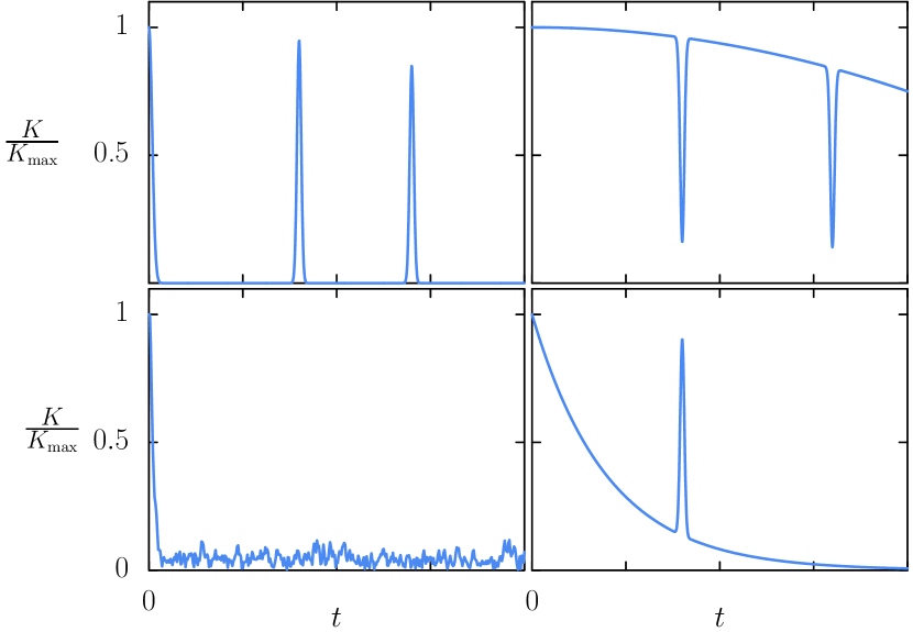
Figure 1: Schematic examples of $K(t)/K_{\text{max}}$ to be considered as QV. (top-left) Example with large $\delta K_{q}$ and $\mathcal{M}^{\langle\cdot\rangle}$, good QV candidate. (top-right) Worst case scenario. Small $\delta K_{q}$, small (or null) $\mathcal{M}^{\langle\cdot\rangle}$ and infromation always available for EVE to grab. (bottom-left) Small $\mathcal{M}^{\langle\cdot\rangle}$ an $\Delta K_{q}$ (poor in for information retrieval) but decent $\mathcal{N}_{q}$ (good for information protection). (bottom-left) More general case, strongly depending on $\mathcal{M}^{\langle\cdot\rangle}$ and the height of the peak at $t_{f}$.

If $\langle K(t)\rangle$ is very large, close to $K_{\text{max}}$ (e.g. Fig. 1 top-right), then, by definition, the channel is not a good QV: a large proportion of the information is readily available at all times before $t_{f}$. Here $K(t_{f})<\langle K\rangle$ (so Eq. (11) does not hold), but the only possibility to have good efficiency is the trivial $q\to 0$ case. If, on the other hand, $\langle K(t)\rangle$ and $K(t_{f})$ are both very small (Fig. 1 bottom-left) – again $\mathcal{M}^{\langle\cdot\rangle}\approx 0$– there is little chance to retrieve the information, even for small $q$, yielding poor efficiency and $\mathcal{N}_{q}$. For large $q$, $\mathcal{N}_{q}\approx qK_{\text{max}}$ can be large. The interpretation of this large value of $\mathcal{N}_{q}$ is that Eve will likely attack, but unsucceesfully. Here the interpretation of this large value of $\mathcal{N}_{q}$ is that Eve will likely attack, but unsucceesfully. Finally, we consider the case where $K(t)$ decays monotonously except for one bump (e.g. Fig. 1 bottom-right). The analysis now requires a little more care. If $K(t_{f})<\langle K\rangle$, which happens for a small enough bump, then $\mathcal{M}^{\cdot}_{\mathcal{K}}=0$, and there is no connection between $\Delta K_{q}$ (or $\mathcal{N}_{q}$) and $\mathcal{M}^{\cdot}_{\mathcal{K}}$. The analysis is similar to that of Fig. 1 (top-right). On the other hand if $\mathcal{M}^{\langle\cdot\rangle}>0$ the efficiency is bounded by Eq. (11) and for maximum $\mathcal{M}^{\langle\cdot\rangle}$, the case is equivalent to the first one (top-left).

IV Examples

In this section we present concrete physical examples of quantum channels where we can test the newly proposed measures and their relation with the QV scheme.

IV.1 Environment with mixed dynamics

Let us discuss encoding quantum information in a qubit coupled to an environment in a dephasing manner. We consider that the environment evolves according to a dynamics that in the semiclassical limit is mixed, i.e. has integrable and chaotic regions in phase space.

A simple way to realize such environment is using a controlled kicked quantum map García-Mata et al. (2012, 2014). In this case, the environment evolution is slightly modified depending on the state of the qubit. This is equivalent to having a coupling with the environment that commutes with the Hamiltonians corresponding to the free evolution of each part, qubit and environment.

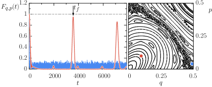
Figure 2: (left) $F(t)$ as a function of time for two different initial states of an environment modeled by the quantum Harper map. (right) the classical phase space of the environment for the parameters studied (see main text). The two states of the environment in the left figure are coherent pure states centered where the color dots are shown in the phase space portrait, i.e. one in the chaotic region (blue) and the other in the integrable region (red), corresponding to similar colors in the left panel.

Here we choose to use the quantum Harper map Leboeuf et al. (1990). The evolution operator, in terms of the discrete conjugate space-momentum variables $\hat{q}$ and $\hat{p}$ is

$$U_{k}=\exp\left[-i\frac{k}{\hbar}\cos(2\pi\hat{p})\right]\exp\left[-i\frac{k}{\hbar}\cos(2\pi\hat{q})\right],$$ (14)

$\hbar\equiv 1/(2\pi N)$ being the effective Planck constant and $N$ the dimension of the Hilbert space of the environment. The corresponding classical dynamics ($N\to\infty$) is given by

$$p_{n+1} =p_{n}-k\sin(2\pi q_{n}),$$

$$q_{n+1} =q_{n}+k\sin(2\pi p_{n+1}).$$ (15)

The phase space geometry is a 2-torus, so $p_{n}$ and $q_{n}$ are taken modulo 1. For $k=0.2$, the dynamics is mixed, see Fig. 2. To use this closed system as an environment, we consider that the state of the qubit induces a small change in the parameter $k$ of the map, so the evolution of the whole system for one time step is given by the Floquet operator

$$U=|0\rangle\!\langle 0|U_{k}+|1\rangle\!\langle 1|U_{k+\delta k}$$ (16)

and $U(t)=U^{t}$, for integer $t$. Throughout this example, we shall set $N=4000$, $k=0.2$ and $\delta k=2\hbar$, unless otherwise stated. The initial state of the whole system is the uncorrelated state $\rho_{\rm sys}\otimes\rho_{{\rm env},q,p}$, where the environment will be taken to be a pure coherent state centered in $(q,p)$. The state of the qubit, obtained with unitary evolution in the whole system and partial tracing the environment, is given by

$$\rho_{\rm sys}(t)=\mathop{\mathrm{tr}}\nolimits_{\rm env}\left[U(t)\rho_{\rm sys}\otimes\rho_{{\rm env},q,p}U^{\dagger}(t)\right]=\Lambda^{q,p}_{t}(\rho_{\rm sys}).$$ (17)

In the basis of Pauli matrices $\{\sigma_{i}\}=\{\mathbb{I},\sigma_{x},\sigma_{y},\sigma_{z}\}/\sqrt{2}$, the induced channel takes the form

$$\Lambda_{q,p}(t)=\begin{pmatrix}1&0&0&0\\ 0&{\rm Re}[f_{q,p}(t)]&{\rm Im}[f_{q,p}(t)]&0\\ 0&{\rm Im}[f_{q,p}(t)]&{\rm Re}[f_{q,p}(t)]&0\\ 0&0&0&1\end{pmatrix},$$ (18)

where

$$f_{q,p}(t)=\mathop{\mathrm{tr}}\nolimits\left[\rho_{{\rm env},q,p}U_{k+\delta k}(t)^{\dagger}U_{k}(t)\right]$$ (19)

is the expectation value of the echo operator $U_{k+\delta k}(t)^{\dagger}U_{k}(t)$ with respect to the corresponding coherent state (also known as fidelity amplitude). We shall also define the fidelity, $F_{q,p}(t)=|f_{q,p}(t)|$, for later convenience. Notice that the channel depends, up to unitary operations, only on $F_{q,p}(t)$, and thus all capacities will be functions solely of this quantity.

In Fig. 2 (left) we show two examples of $F_{q,p}(t)$, for different initial conditions of the environment (marked with circles in Fig. 2 (right). One can see that in case the environment starts inside the chaotic sea, the system has very small $\mathcal{M}^{\langle\cdot\rangle}_{F}$ and $\mathcal{M}^{\text{max}}_{F}$ and therefore from Eq. (12), it will be a very bad QV.

An interesting point of Fig. 2 is how $\mathcal{M}^{\langle\cdot\rangle}_{F}$ and $\mathcal{M}^{\text{max}}_{F}$ compare to $\mathcal{M}^{\text{BLP}}$ and $\mathcal{M}^{\text{RHP}}$.

	$\mathcal{M}^{\langle\cdot\rangle}_{F}$	$\mathcal{M}^{\rm max}_{F}$	$\mathcal{M}^{\rm BLP}$	$\mathcal{M}^{\rm RHP}$
$\bullet$	0.899	0.953	6.6	1333.97
$\bullet$	0.108	0.194	125.84	6274.89

Table 1: Comparison between different values of measures of non-markovianity for the two situations depicted in fig. 2, with corresponding colors. We cut the integral in eq. (20) in $t=8000$. The inherent fluctuations present for this finite dimensional environment cause the integrable situation (with larger fluctuations) to reach larger values for the NM measures $\mathcal{M}^{\rm BLP}$ and $\mathcal{M}^{\rm RHP}$, than the chaotic counterpart. On the other hand, both $\mathcal{M}^{\langle\cdot\rangle}_{F}$ and $\mathcal{M}^{\rm max}_{F}$ capture well the idea of QV, reporting large values for the integrable case, and small values for the chaotic one.

In terms of $F_{q,p}(t)$ the latter are given by

$$\mathcal{M}^{\text{BLP}} =2\int_{0,\dot{F}>0}^{t_{\mathrm{cut}}}d\tau\dot{F}_{q,p}(\tau),$$

$$\mathcal{M}^{\text{RHP}} =\int_{0,\dot{F}>0}^{t_{\mathrm{cut}}}d\tau\frac{\dot{F}_{q,p}(\tau)}{F_{q,p}(\tau)},$$ (20)

where $t_{\mathrm{cut}}$ indicates a cutoff time. The $[F_{q,p}(\tau)]^{-1}$ term in $\mathcal{M}^{\text{RHP}}$ can be problematic when $F_{q,p}(\tau)$ is very small, which is exactly the case for an initial state located in the chaotic region. In Table 1 the values of all four measures, based on $F$, corresponding to Fig. 2 are shown. The values reported in the table highlight important characteristics of all four measures. On the one hand, for non-monotonicity based measures, intuitively we expect that a fast decaying $K(t)$ followed by sharp, and high revivals would yield a larger value of non-Markovianity. This is not the case for $\mathcal{M}^{\text{BLP}}$ and $\mathcal{M}^{\text{RHP}}$ (at least in this particular example), for different reasons. In the case of $\mathcal{M}^{\text{RHP}}$ it is due to the small denominator and in the case of $\mathcal{M}^{\text{BLP}}$ it is due to fluctuations (and finite $N$). These facts are further illustrated in the color density plots of Fig. 3. We see that in all cases the underlying classical structure is clearly outlined. For both $\mathcal{M}^{\langle\cdot\rangle}_{F}$ and $\mathcal{M}^{\text{max}}_{F}$ an additional structure appears that resembles the unstable manifolds. The measures $\mathcal{M}^{\langle\cdot\rangle}_{F}$, $\mathcal{M}^{\text{max}}_{F}$, and $\mathcal{M}^{\text{BLP}}$ all seem to peak in the vicinity of the border between chaotic and regular behavior. As stated before, the $\mathcal{M}^{\text{RHP}}$ measure behaves differently, as it is larger in the chaotic region.

Notice that the measure $M^{\langle\cdot\rangle}_{F}$ can be associated with the task of transmitting classical information (without the use of entanglement) encoded initially in the states $|\pm\rangle$.

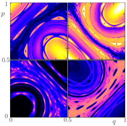
Figure 3: (Color online) Mapping of classical phase space obtained from the different non-Markovianity measures discussed, for the quantum Harper map with $N=8000$, $K=0.2$, $\delta K/\hbar=2$ and maximum time $t_{\mathrm{cut}}=16000$. The color code is dark/black$=0$, light/white$=$ max. The different subfigures correspond to $\mathcal{M}^{\langle\cdot\rangle}_{F}$, top left with a maximum value of the measure of $1$; $\mathcal{M}^{\text{max}}_{F}$ on the top right with maximum value of $1$; $\mathcal{M}^{\rm BLP}$, bottom left, with a maximum value of $400$; and at the bottom right, $\mathcal{M}^{\rm RHP}$ with a maximum value of $19000$.

IV.2 Non markovian Jaynes-Cummings model

In order to explore and compare the different measures of non-Markovianity discussed throughout this work, we now consider the paradigmatic Jaynes-Cummings model Jaynes and Cummings (1963), which has served as testbed in quantum optics; see e.g. Breuer and Petruccione (2007). In this model, a two level atom is coupled to a bosonic bath, which induces a degradable channel in the qubit. We shall take advantage of the fact that a lot is known about this model analytically and we will build upon known results.

The Hamiltonian of the system is $H=H_{0}+H_{I}$, where $H_{0}$ is the free Hamiltonian of the atom plus the reservoir and $H_{I}$ the interaction between them. In particular, $H_{0}=\omega_{0}\sigma_{+}\sigma_{-}+\sum_{k}\omega_{k}b_{k}^{\dagger}b_{k}$, where $\sigma_{\pm}$ are the rising and lowering operators in the atom, $\omega_{0}$ is the energy difference between the two levels in the atom, $b_{k}$ and $b_{k}^{\dagger}$ are creation and annihilation operators of mode $k$ of the bath, and $\omega_{k}$ its frequency. The interaction Hamiltonian is given by $H_{I}=\sigma_{+}\otimes B+\sigma_{-}\otimes B^{\dagger}$, with $B=\sum_{k}g_{k}b_{k}$ and $g_{k}$ the coupling of the qubit to mode $k$. In the limit of an infinite number of reservoir oscillators and a smooth spectral density, this model leads to the following channel Breuer and Petruccione (2007):

$$\Lambda_{t}\left[\rho\right]=\left(\begin{array}[]{cc}1-|G(t)|^{2}\rho_{ee}&G(t)\rho_{ge}\\ G^{*}(t)\rho_{ge}^{*}&|G(t)|^{2}\rho_{ee}\end{array}\right),$$ (21)

where the initial state $\rho=\begin{pmatrix}1-\rho_{ee}&\rho_{ge}\\ \rho_{ge}^{*}&\rho_{ee}\\ \end{pmatrix}$.

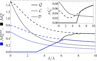
Figure 4: Comparative results of the measures of quantum non Markovianity treated in this work for the Jaynes-Cummings model, as a function of the scaled detuning $\delta/\lambda$, with a coupling of $\gamma=20\lambda$. We show three different types of measures, $\mathcal{M}^{\infty}_{\mathcal{K}}$ (black lines), $\mathcal{M}^{\max{}}_{\mathcal{K}}$ (blue lines), and $\mathcal{M}^{\langle\cdot\rangle}_{\mathcal{K}}$ (inset) for three different capacities: Quantum capacity $\mathcal{Q}$ (solid lines), classical entanglement assisted capacity $\mathcal{C}$ (dashed lines), and the capacity based on distinguishability $\mathcal{D}$ (dotted lines).

The function $G(t)$ is the solution to the equation $\dot{G}(t)=-\int_{0}^{t}d\tau f(t-\tau)G(\tau)$, with $G(0)=1$, and $f(t-\tau)$ is the two-point correlation function of the reservoir. For a Lorenzian spectral density

$$f(t)=\frac{1}{2}\gamma_{0}\lambda e^{-|t|\left(\lambda-i\delta\right)},$$ (22)

we find find

$$G(t)=e^{-\frac{1}{2}t(\lambda-i\delta)}\left[\frac{(\lambda-i\delta)}{\Omega}\sinh\left(\frac{\Omega t}{2}\right)+\cosh\left(\frac{\Omega t}{2}\right)\right],$$ (23)

where $\Omega=\sqrt{-2\gamma\lambda+(\lambda-i\delta)^{2}}$. Here, $\gamma_{0}$ is the strength of the system-reservoir coupling, $\lambda$ is the spectral width, and $\delta$ is the detuning between the peak frequency of the spectral density and the transition frequency of the atom .

In what follows, we study the NM measures $\mathcal{M}_{\mathcal{K}}^{\infty}$, $\mathcal{M}_{\mathcal{K}}^{\max{}}$, and $\mathcal{M}_{\mathcal{K}}^{\langle\cdot\rangle}$ for the capacities $\mathcal{Q}$ (quantum capacity), $\mathcal{C}$ (entanglement-assisted classical capacity), and $\mathcal{D}$ (distinguishability of the states $|\pm\rangle$). The quantum capacity is defined as the maximal amount of quantum information (per channel use, measured as the number of qubits) that can be reliably transmitted through the channel. It is given explicitly in terms of the following maximization Giovannetti and Fazio (2005): $\max_{p\in[0,1]}\{H_{2}\left(|G(t)|^{2}p\right)-H_{2}\left((1-|G(t)|^{2})p\right)\}$ for $|G(t)|^{2}>1/2$ and 0 for $|G(t)|^{2}\leq 1/2$. The entanglement-assisted classical capacity $\mathcal{C}$ is defined as the maximal amount of classical information (per channel use, measured as the number of classical bits) that can be reliably transmitted through the channel, when Alice and Bob are allowed to use an arbitrary number of shared entangled states Smith . For the present channel it is given by Giovannetti and Fazio (2005): $\mathcal{C}=\max_{p\in[0,1]}\{H_{2}(p)+H_{2}\left(|G(t)|^{2}p\right)-H_{2}\left((1-|G(t)|^{2})p\right)\}$. Finally, we also consider the BLP measure defined in Eq. (4). In this case the initial states which maximize the various types of NM measures may be chosen invariably as the two eigenstates of the Pauli matrix $\sigma_{x}$ Breuer (2012). Thereby, we obtain $K(t)=|G(t)|$.

Figure 5: Quantum capacities of the non markovian Jaynes-Cummings model with a strong coupling $\gamma/\lambda=1000$. The solid curves correspond to $\delta/\lambda=0$ (black), $\delta/\lambda=40$ (blue). The dashed curves are $\delta/\lambda=80$ (black), $\delta/\lambda=150$ (blue).

Figure 4 shows a comparison between the measures $\mathcal{M}_{\mathcal{K}}^{\langle\cdot\rangle}$ and $\mathcal{M}_{\mathcal{K}}^{\max{}}$, introduced in this work, and their counterpart $\mathcal{M}^{\infty}_{\mathcal{K}}$. The measures regarding the average $\mathcal{M}_{\mathcal{K}}^{\langle\cdot\rangle}$ are notoriously smaller than the measures regarding both the maximum revival and the integrated revivals. In fact, we find that $\mathcal{M}^{\langle\cdot\rangle}_{\mathcal{K}}\leq\mathcal{M}^{\max{}}_{\mathcal{K}}$, in agreement with (7), and $\mathcal{M}^{\max{}}_{\mathcal{K}}\leq\mathcal{M}^{\infty}_{\mathcal{K}}$. The measures related to the BLP criterion (dotted lines) behave similarly in all three cases, decaying monotonously with $\delta/\lambda$. In the case of the entanglement assisted classical capacity, $\mathcal{M}_{\mathcal{C}}^{\infty}$ and $\mathcal{M}_{\mathcal{C}}^{\max{}}$ also decay monotonously. However, $\mathcal{M}_{\mathcal{C}}^{\langle\cdot\rangle}$ has a minimum at $\delta/\lambda\approx 3$. Beyond that point $\mathcal{M}_{\mathcal{C}}^{\langle\cdot\rangle}$ increases a bit further, but finally decays to zero. In this region, $\mathcal{M}_{\mathcal{C}}^{\langle\cdot\rangle}=\mathcal{M}_{\mathcal{Q}}^{\langle\cdot\rangle}$ which is shown in Fig. 6. The measures related to the quantum capacity (solid lines) show the most complicated behavior. $\mathcal{M}_{\mathcal{Q}}^{\infty}$ and $\mathcal{M}_{\mathcal{Q}}^{\max{}}$ are equal to zero until $\delta/\lambda\approx 3$, $\mathcal{M}_{\mathcal{Q}}^{\langle\cdot\rangle}$ is equal to zero until $\delta/\lambda\approx 5$. Beyond these points, the measures increase linearly. From $\delta/\lambda\approx 6.5$ on, $\mathcal{M}_{\mathcal{Q}}^{\max{}}$ and $\mathcal{M}_{\mathcal{Q}}^{\langle\cdot\rangle}$ reach the corresponding curves for the classical capacity. For somewhat larger values of $\delta/\lambda$ this also happens for the $\mathcal{M}_{\mathcal{Q}}^{\infty}$.

The fact that for quantum capacities, $\mathcal{M}_{\mathcal{Q}}^{\infty}$ and $\mathcal{M}_{\mathcal{Q}}^{\max}$ start to deviate from zero at the same point $\delta/\lambda\approx 3$, illustrates eq. (8). Other interesting feature that can be appreciated in $\mathcal{M}_{\mathcal{Q}}^{\infty}$ are the multiple discontinuities in the derivative with respect to the detuning. This is due to the sudden appearance of new bumps in the quantum capacity of the channel, to which this measure is sensible. Moreover, for most instances of $\mathcal{K}$, $\mathcal{M}_{\mathcal{K}}^{\infty}$ can be discontinuous in the space of finite quantum processes, if we consider the maximum-norm, so the measures are not stable with respect to small deviations in the quantum dynamics. In particular, small amplitude high frequency noise can make $\mathcal{M}_{\mathcal{K}}^{\infty}$ increase arbitrarily, whereas, it has a small effect (proportional to the amplitude) in the case of $\mathcal{M}_{\mathcal{K}}^{\langle\cdot\rangle}$ and $\mathcal{M}_{\mathcal{K}}^{\max{}}$.

Regarding the classical capacity, it is worth noticing that the different cases do not share the same tendency, $\mathcal{M}_{\mathcal{C}}^{\max{}}$ and $\mathcal{M}_{\mathcal{C}}^{\infty}$ diminishes with the detuning (as opposed to the quantum capacity cases), but $\mathcal{M}_{\mathcal{C}}^{\langle\cdot\rangle}$ has a non monotonic behavior, mimicking fidelity until $\delta/\lambda\approx 3$, and then resembling the quantum capacity. A direct consequence inherited from the fact that $\mathcal{Q}\leq\mathcal{C}$ is that $\mathcal{M}_{\mathcal{Q}}^{\ \cdot}\leq\mathcal{M}_{\mathcal{C}}^{\ \cdot}$ as can be seen from the fact that, for all colors, the dashed line bounds the continuous line (here, the dot denotes any of $\max{}$, $\langle\cdot\rangle$ or $\infty$). As a general remark, we also observe that $\mathcal{M}_{\mathcal{K}}^{\langle\cdot\rangle}$ is much smaller than $\mathcal{M}_{\mathcal{K}}^{\max{}}$ and $\mathcal{M}_{\mathcal{K}}^{\infty}$. This is due to the fact that the peaks in the different capacities are thick, and the system, in fact, would not serve as a good quantum vault.

Figure 5 shows the evolution of several quantum capacities for the Jaynes-Cummings model varying the detuning, while keeping the reservoir coupling fixed. The table 2 shows the values of the corresponding measures of non-Markovianity treated in this work. It shows that large detunings lead to poor scenarios for a quantum vault operation, while for zero and small detuning there are better situations for a usage of the QV. The time when the first peak in the capacity appears can be tuned by choosing the correlation time of the bath. The figure 6 shows a density plot of the non-Markovianity measures, $\mathcal{M}^{\langle\cdot\rangle}_{\mathcal{Q}}$, as a function of the channel parameters $\delta$ and $\gamma$. It shows how a region of high $\mathcal{M}^{\langle\cdot\rangle}_{\mathcal{Q}}$ appears as the coupling increases, as long as the detuning is not too strong ($\sim 10$). This is because large couplings induce a rapid decay in the quantum capacity while the oscillations from the detuning restore the capacity. For large detunings, the probability for transitions in the atom is low, which implies that the capacity initially has small oscillations close to one with and a slow decay. For small couplings $\gamma/\lambda<1/2$ and zero detuning, the capacity decays monotonically Bylicka et al. (2014), this makes all the measures discussed equal to zero and therefore a useless QV.

	$\delta/\lambda$	$\mathcal{M}^{\langle\cdot\rangle}_{\mathcal{Q}}$	$\mathcal{M}^{\rm max}_{\mathcal{Q}}$	$\mathcal{M}_{\mathcal{Q}}^{\infty}$
—	0	0.4072	0.6419	1.4322
—	40	0.4301	0.8154	4.4928
$---$	80	0.2564	0.4963	6.0953
$---$	150	0.1210	0.2309	4.7588

Table 2: The table shows the measures treated in this work of the quantum capacities shown in figure 5, with $t_{\mathrm{cut}}{}=\infty$.

Figure 6: Density plot of the $\mathcal{M}^{\langle\cdot\rangle}_{\mathcal{Q}}$ for the non Markovian Jaynes-Cummings model as a function of its parameters.

V Conclusions

In the light of considerable advances in the experimental manipulation of quantum systems at the very fundamental level, understanding and controlling how a quantum system interacts with its surroundings is of paramount importance. In this context finite, structure rich environments play an important role, and the challenge has been to understand and control the resulting non-Markovian evolution. In particular, one might wonder whether there is a possibility to take advantage of the flow of information back to the system which is characteristic to non-Markovianity. Defining and quantifying non-Markovianity is a non-trivial task. In this work we have shown that one can define and quantify non-Markovian behavior in a physically meaningful way. One that is insightful and avoids the drawbacks of previous attempts, like divergence in very generic cases, and counter intuitive outcomes. Moreover we could define the new measure with a task in mind: hiding and retrieving classical or quantum information using a quantum channel. The efficiency with which this taks is accomplished, is directly related to the NM measure. Finally, we have illustrated the proposed measures with simple physical examples.