T-PHOT: A new code for PSF-matched, prior-based, multiwavelength extragalactic deconfusion photometry

Abstract

Context. The advent of deep multiwavelength extragalactic surveys has led to the necessity for advanced and fast methods for photometric analysis. In fact, codes which allow analyses of the same regions of the sky observed at different wavelengths and resolutions are becoming essential to thoroughly exploit current and future data. In this context, a key issue is the confusion (i.e. blending) of sources in low-resolution images.

Aims. We present t-phot, a publicly available software package developed within the astrodeep project. t-phot is aimed at extracting accurate photometry from low-resolution images, where the blending of sources can be a serious problem for the accurate and unbiased measurement of fluxes and colours.

Methods. t-phot can be considered as the next generation to tfit, providing significant improvements over and above it and other similar codes (e.g. convphot). t-phot gathers data from a high-resolution image of a region of the sky, and uses this information (source positions and morphologies) to obtain priors for the photometric analysis of the lower resolution image of the same field. t-phot can handle different types of datasets as input priors, namely i) a list of objects that will be used to obtain cutouts from the real high-resolution image; ii) a set of analytical models (as .fits stamps); iii) a list of unresolved, point-like sources, useful for example for far infrared wavelength domains.

Results. By means of simulations and analysis of real datasets, we show that t-phot yields accurate estimations of fluxes within the intrinsic uncertainties of the method, when systematic errors are taken into account (which can be done thanks to a flagging code given in the output). t-phot is many times faster than similar codes like tfit and convphot (up to hundreds, depending on the problem and the method adopted), whilst at the same time being more robust and more versatile. This makes it an excellent choice for the analysis of large datasets. When used with the same parameter sets as for tfit it yields almost identical results (although in a much shorter time); in addition we show how the use of different settings and methods significantly enhances the performance.

Conclusions. t-phot proves to be a state-of-the-art tool for multiwavelength optical to far-infrared image photometry. Given its versatility and robustness, t-phot can be considered the preferred choice for combined photometric analysis of current and forthcoming extragalactic imaging surveys.

1 Introduction

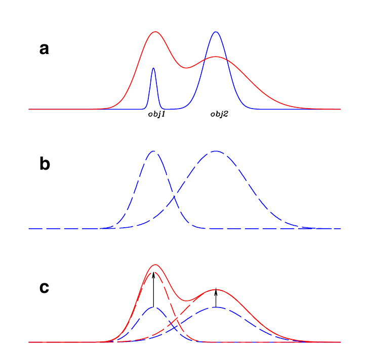
Figure 1: Schematic representation of the PSF-matched algorithm implemented in t-phot. Top: two objects are clearly detected and separated in the high-resolution detection image (blue line). The same two objects are blended in the low-resolution measurement image and have different colours (red line). Middle: the two objects are isolated in the detection image and are individually smoothed to the PSF of the measurement image, to obtain normalized model templates. Bottom: the intensity of each object is scaled to match the global profile of the measurement image. The scaling factors are found with a global $\chi^{2}$ minimization over the object areas. Image from De Santis et al. (2007).

Combining observational data from the same regions of the sky in different wavelength domains has become common practice in the past few years (e.g. Agüeros et al. 2005; Obrić et al. 2006; Grogin et al. 2011, and many others). However, the use of both space-based and ground-based imaging instruments, with different sensitivities, pixel scales, angular resolutions, and survey depths, raises a number of challenging difficulties in the data analysis process.

In this context, it is of particular interest to obtain detailed photometric measurements for high-redshift galaxies in the near-infrared (NIR; corresponding to rest-frame optical) and far-infrared (FIR) domains. In particular, great attention must be paid to bandpasses containing spectral features which allow a thorough investigation of the sources, disentangling degenerate observational features, and obtaining crucial clues to the understanding of the galactic physics (e.g. Daddi et al. 2004; Fontana et al. 2009). At $z>3$, for example, photometry longward of $H$-band is needed to locate and measure the size of the Balmer break. A passive galaxy at $z\simeq 6$ (with the Balmer break lying longward of the $K$-band) can have $H$-band and $3.6\mu$m fluxes compatible, for example, with a star forming, dusty galaxy at $z\simeq 1$, and $K-$band photometry is necessary in order to disentangle the degeneracy. However, the limited resolution of the ground based $K-$band observations can impose severe limits on the reliability of traditional aperture or even Point Spread Function (PSF) fitting photometry. In addition, IRAC photometry is of crucial importance so that reliable photometric redshifts of red and high-$z$ sources can be obtained, and robust stellar mass estimates can be derived.

To address this, a high-resolution image (HRI), for example obtained from the Hubble Space Telescope in the optical domain, can be used to retrieve detailed information on the positions and morphologies of the sources in a given region of the sky. Such information can be subsequently used to perform the photometric analysis of the lower resolution image (LRI), using the HRI data as priors. However, simply performing aperture photometry on the LRI at the positions measured in the HRI can be dramatically affected by neighbour contamination for reasonably sized apertures. On the other hand, performing source extraction on both images and matching the resulting catalogues is compromised by the inability to deblend neighbouring objects, and may introduce significant inaccuracies in the cross-correlation process. PSF-matching techniques that degrade high-resolution data to match the low-resolution data discard much of the valuable information obtained in the HRI, reducing all images to the “lowest common denominator” of angular resolution. Moreover, crowded-field, PSF-fitting photometry packages such as daophot (Stetson 1987) perform well if the sources in the LRI are unresolved, but are unsuitable for analysis of even marginally resolved images of extragalactic sources.

A more viable approach consists of taking advantage of the morphological information given by the HRI, in order to obtain high-resolution cutouts or models of the sources. These priors can then be degraded to the resolution of the LRI using a suitable convolution kernel, constructed by matching the PSFs of the HRI and of the LRI. Such low-resolution templates, normalized to unit flux, can then be placed at the positions given by the HRI detections, and the multiplicative factor that must be assigned to each model to match the measured flux in each pixel of the LRI will give the measured flux of that source. Such an approach, although relying on some demanding assumptions as described in the following sections, has proven to be efficient. It has been implemented in such public codes as tfit (Laidler et al. 2007) and convphot (De Santis et al. 2007), and has already been utilized successfully in previous studies (e.g. Guo et al. 2013; Galametz et al. 2013).

In this paper we describe a new software package, t-phot, developed at INAF-OAR as part of the astrodeep project. The t-phot software can be considered a new, largely improved version of tfit, supplemented with many of the features of convphot. Moreover, it adds many important new options, including the possibility of adopting different types of priors (namely real images, analytical models, or point-sources). In particular, it is possible to use t-phot on FIR and sub-millimetric (sub-mm) datasets, as a competitive alternative to the existing dedicated software such as FastPhot (Béthermin et al. 2010) and DesPhot (Roseboom et al. 2010; Wang et al. 2014). This makes t-phot a versatile tool, suitable for the photometric analysis of a very broad range of wavelengths from UV to sub-mm.

t-phot is a robust and easy-to-handle code, with a precise structural architecture (a Python envelope calling C/C++ core codes) in which different routines are encapsulated, implementing various numerical/conceptual methods, to be chosen by simple switches in a parameter file. While a standard default “best choice” mode is provided and suggested, the user is allowed to select a preferred setting.

One of the main advantages of t-phot is a significant saving of computational time with respect to both tfit and convphot (see Sect. 5). This has been achieved with the use of fast C modules and an efficient structural arrangement of the code. In addition to this, we demonstrate how different choices of parameters influence the performace, and can be optimized to significantly improve the final results with respect to tfit, for example.

The plan of the paper is as follows. Sect. 2 provides a general introduction to the code, its mode of operation and its algorithms. In Section 3 we discuss some assumptions, limitations and caveats of the method. Section 4 presents a comprehensive set of tests, based on simulated and real datasets, to assess the performance of the code and to fully illustrate its capabilities and limitations. Section 5 briefly discusses the computational performances of t-phot and provides some reference computational timescales. Finally, in Section 6 the key features of t-phot are summarized, and outstanding issues and potential complications are briefly discussed.

2 General description of the code

As described above, t-phot uses spatial and morphological information gathered from a HRI to measure the fluxes in a LRI. To this end, a linear system is built and solved via matricial computing, minimizing the $\chi^{2}$ (in which the numerically determined fluxes for each detected source are compared to the measured fluxes in the LRI, summing the contributions of all pixels). Moreover, the code produces a number of diagnostic outputs and allows for an iterative re-calibration of the results. Figure 1 shows a schematic depiction of the basic PSF-matched fitting algorithm used in the code.

As HRI priors t-phot can use i) real cutouts of sources from the HRI, ii) models of sources obtained with Galfit or similar codes, iii) a list of coordinates where PSF-shaped sources will be placed, or a combination of these three types of priors.

For a detailed technical description of the mode of operation of the code, we refer the reader to the Appendix and to the documentation included in the downloadable tarball. Here, we will briefly describe its main features.

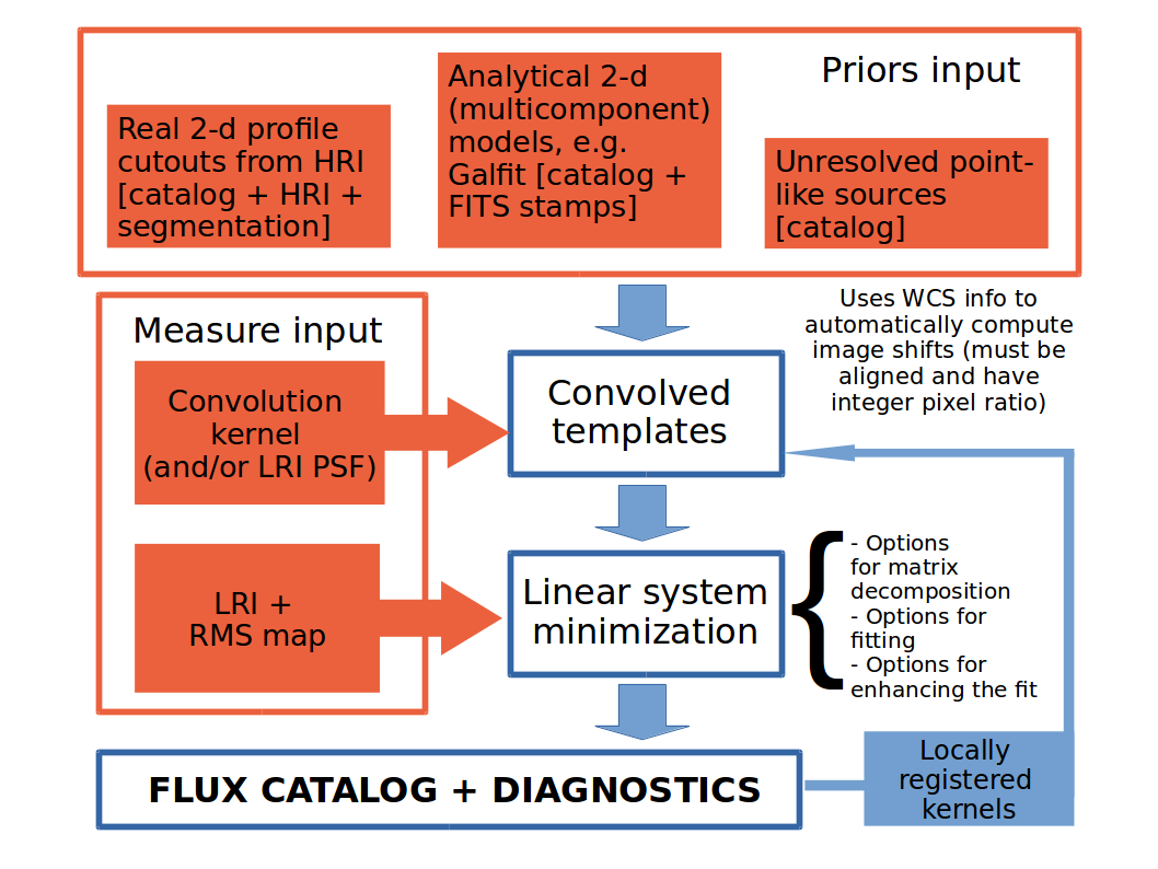
Figure 2: Schematic representation of the workflow in t-phot.

2.1 Pipeline

The pipeline followed by t-phot is outlined in the flowchart given in Fig. 2. The following paragraphs give a short description of the pipeline.

2.1.1 Input

The input files needed by t-phot vary depending on the type(s) of priors used.

If true high-resolution priors are used, e.g. for optical/NIR ground-based or IRAC measurements using Hubble Space Telescope (HST) cutouts, t-phot needs

• the detection, high-resolution image (HRI) in .fits format;

• the catalogue of the sources in the HRI, obtained using SExtractor or similar codes (the required format is described in Appendix A);

• the segmentation map of the HRI, in .fits format, again obtained using SExtractor or similar codes, having the value of the id of each source in the pixels belonging to it, and zero everywhere else;

• a convolution kernel $K$, in the format of a .fits image or of a .txt file, matching the PSFs of the HRI and the LRI so that $PSF_{LRI}=K*PSF_{HRI}$ ($*$ is the symbol for convolution). The kernel must have the HRI pixel scale.

If analytical models are used as priors (e.g. Galfit models), t-phot needs

• the stamps of the models (one per object, in .fits format);

• the catalogue of the models (the required format is described in Appendix A);

• the convolution kernel $K$ matching the PSFs of the HRI and the LRI, as in the previous case.

If models have more than one component, one separate stamp per component and catalogues for each component are needed (e.g. one catalogue for bulges and one catalogue for disks).

If unresolved, point-like priors are used, t-phot needs

• the catalogue of positions (the required format is described in Appendix A);

• the LRI PSF, in the LRI pixel scale.

In this case, a potential limitation to the reliability of the method is given by the fact that the prior density usually needs to be optimized with respect to FIR/sub-mm maps, as discussed in Shu et al. (2015, in preparation) and Elbaz et al. (2011) (see also Wang et al. 2015; Bourne et al. 2015, in preparation). The optimal number of priors turns out to be around 50-75% of the numbers of beams in the map. The main problem is identifying which of the many potential priors from, for example, an HST catalogue one should use. This is a very complex issue and we do not discuss it in this paper.

If mixed priors are used, t-phot obviously needs the input files corresponding to each of the different types of priors in use.

Finally, in all cases t-phot needs

• the measure LRI, background subtracted (see next paragraph), in .fits format, with the same orientation as the HRI (i.e. no rotation allowed); the pixel scale can be equal to, or an integer multiple of, the HRI pixel scale, and the origin of one pixel must coincide; it should be in surface brightness units (e.g. counts/s/pixel, or Jy/pixel for FIR images, and not PSF-filtered);

• the LRI RMS map, in .fits format, with the same dimensions and WCS of the LRI.

Table 1 summarizes the input requirements for the different choices of priors just described.

	Real cutouts	Analytical models	Point-sources
Priors	HRI Segmentation Catalogue	HRI Model Stamps Catalogue	Positions Catalogue
Transformation	Convolution Kernel	Convolution Kernel	PSFLRI
Measure	LRI RMSLRI	LRI RMSLRI	LRI RMSLRI

Table 1: The input files needed by t-phot for different settings. See text for details.

All the input images must have the following keywords in their headers: CRPIXn, CRVALn, CDn_n, CTYPEn (n=1,2).

2.1.2 Background subtraction

As already mentioned, the LRI must be background subtracted before being fed to t-phot. This is of particular interest when dealing with FIR/sub-mm images, where the typical standard is to use zero-mean. To estimate the background level in optical/NIR images, one simple possibility is to take advantage of the option to fit point-like sources to measure the flux for a list of positions chosen to fall within void regions. The issue is more problematic in such confusion-limited FIR images where there are no empty sky regions. In such cases, it is important to separate the fitted sources (those listed in the prior catalogue) from the background sources, which contribute to a flat background level behind the sources of interest. The priors should be chosen so that these two populations are uncorrelated. The average contribution of the faint background source population can then be estimated for example by i) injecting fake sources into the map and measuring the average offset (output-input) flux, or ii) measuring the modal value in the residual image after a first pass through t-phot (see e.g. Bourne et al. 2015, in preparation).

2.1.3 Stages

t-phot goes through “stages”, each of which performs a well-defined task. The best results are obtained by performing two runs (“pass 1” and “pass 2”), the second using locally registered kernels produced during the first. The possible stages are the following:

• priors: creates/organizes stamps for sources as listed in the input priors catalogue(s);

• convolve: convolves each high-resolution stamp with the convolution kernel $K$ to obtain models (“templates”) of the sources at LRI resolution. The templates are normalized to unit total flux. If the pixel scale of the images is different, transforms templates accordingly. Convolution is preferably performed in Fourier space, using fast FFTW3 libraries; however the user can choose to perform it in real pixel space, ensuring a more accurate result at the expense of a much slower computation.

• positions: if an input catalogue of unresolved sources is given, creates the PSF-shaped templates listed in it, and merges it with the one produced in the convolve stage;

• fit: performs the fitting procedure, solving the linear system and obtaining the multiplicative factors to match each template flux with the measured one;

• diags: selects the best fits and produces the final formatted output catalogues with fluxes and errors, plus some other diagnostics, see Sect. 2.3;

• dance: obtains local convolution kernels for the second pass; it can be skipped if the user is only interested in a single-pass run;

• plotdance: plots diagnostics for the dance stage; it can be skipped for any purpose other than diagnostics;

• archive: archives all results in a subdirectory whose name is based on the LRI and the chosen fitting method (to be used only at the end of the second pass).

The exact pipeline followed by the code is specified by a keyword in the input parameter file. See also Appendix A for a more detailed description of the whole procedure.

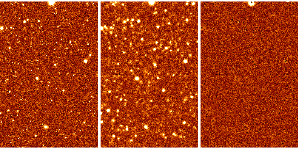
Figure 3: Example of the results of a standard t-phot run using extended priors. Left to right: HRI (FWHM=0.2”), LRI (FWHM=1.66”), and residuals image for a simulated dataset. LRI and residual image are on the same greyscale.

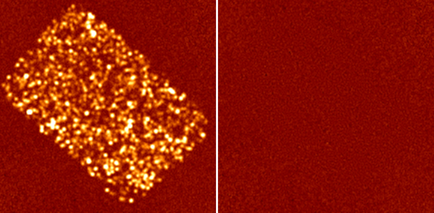
Figure 4: Example of the results of a standard t-phot run using point-source priors. Left to right: LRI (FWHM=25”) and residuals image (same greyscale) for a simulated dataset. See also Sect. 4.1.2.

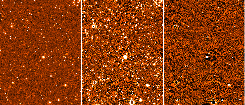
Figure 5: Example of the results of a standard t-phot run using analytical priors. Left to right: CANDELS COSMOS $H$-band (HRI), $R$-band (LRI) and residuals image obtained using Galfit two-component models. LRI and residual image are on the same greyscale.

2.1.4 Solution of the linear system

The search for the LRI fluxes of the objects detected in the HRI is performed by creating a linear system

$$\sum_{m,n}I(m,n)=\sum_{m,n}\sum_{i}^{N}F_{i}P_{i}(m,n)$$ (1)

where $m$ and $n$ are the pixel indexes, $I$ contains the pixel values of the fluxes in the LRI, $P_{i}$ is the normalized flux of the template for the $i$-th objects in the (region of the) LRI being fitted, and $F_{i}$ is the multiplicative scaling factor for each object. In physical terms, $F_{i}$ represents the flux of each object in the LRI (i.e. it is the unknown to be determined).

Once the normalized templates for each object in the LRI (or region of interest within the LRI) have been generated during the convolve stage, the best fit to their fluxes can be simultaneously derived by minimizing a $\chi^{2}$ statistic,

$$\chi^{2}=\left[\frac{\sum_{m,n}I(m,n)-M(m,n)}{\sigma(m,n)}\right]^{2}$$ (2)

where $m$ and $n$ are the pixel indexes,

$$M(m,n)=\sum_{i}^{N}F_{i}P_{i}(m,n)$$ (3)

and $\sigma$ is the value of the RMS map at the $(m,n)$ pixel position.

The output quantities are the best-fit solutions of the minimization procedure, i.e. the $F_{i}$ parameters and their relative errors. They can be obtained by resolving the linear system

$$\frac{\partial\chi^{2}}{\partial F_{i}}=0$$ (4)

for $i=0,1,...,N$.

In practice, the linear system can be rearranged into a matrix equation,

$$AF=B$$ (5)

where the matrix $A$ contains the coefficients $P_{i}P_{j}/\sigma^{2}$, $F$ is a vector containing the fluxes to be determined, and $B$ is a vector given by $I_{i}P_{i}/\sigma^{2}$ terms. The matrix equation is solved via one of three possible methods as described in the next subsection.

2.1.5 Fitting options

t-phot allows for some different options to perform the fit:

• three different methods for solving the linear system are implemented, namely, the LU method (used by default in tfit), the Cholesky method, and the Iterative Biconjugate Gradient method (used by default in convphot; for a review on methods to solve sparse linear systems see e.g. Davis 2006). They yield similar results, although the LU method is slightly more stable and faster;

• a threshold can be imposed so that only pixels with a flux higher than this level will be used in the fitting procedure (see Sect. 4.1.4);

• sources fitted with a large, unphysical negative flux ($f_{meas}<-3\sigma$, where $\sigma$ is their nominal error, see below) can be excluded from the fit, and in this case a new fitting loop will be performed without considering these sources.

The fit can be performed i) on the entire LRI as a whole, producing a single matrix containing all the sources (this is the method adopted in convphot); ii) subdividing the LRI into an arbitrary grid of (overlapping) small cells, perfoming the fit in each of such cells separately, and then choosing the best fit for each source, using some convenient criteria to select it (because sources will be fitted more than once if the cells overlap; this is the method adopted in tfit); iii) ordering objects by decreasing flux, building a cell around each source including all its potential contaminants, solving the problem in that cell and assigning to the source the obtained flux (cells-on-objects method; see the Appendix for more details).

While the first method is the safest and more accurate because it does not introduce any bias or arbitrary modifications, it may often be unfeasible to process at once large or very crowded images. Potentially large computational time saving is possible using the cells-on-objects method, depending on the level of blending/confusion in the LRI; if it is very high, most sources will overlap and the cells will end up being very large. This ultimately results in repeating many times the fit on regions with dimensions comparable to the whole image (a check is implemented in the code, to automatically change the method from cells-on-objects to single fit if this is the case). If the confusion is not dramatic, a saving in computational time up to two orders of magnitude can be achieved. The results obtained using the cells-on-objects method prove to be virtually identical to those obtained with a single fit on the whole image (see Sect. 4.1.2). On the other hand, using the arbitrary cells method is normally the fastest option, but can introduce potentially large errors to the flux estimates owing to wrong assignments of peripheral flux from sources located outside a given cell to sources within the cell (again, see Sect. 4.1.2 and the Appendix B).

2.1.6 Post-fitting stages: kernel registration

After the fitting procedure is completed, t-phot will produce the final output catalogues and diagnostic images (see Sect. 2.3). Among these, a model image is obtained by adding all the templates, scaled to their correct total flux after fitting, in the positions of the sources. This image will subsequently be used if a second pass is planned; during a stage named dance, a list of positional shifts is computed, and a set of shifted kernels are generated and stored. The dance stage consists of three conceptual steps:

• the LRI is divided into cells of a given size (specified by the keyword dzonesize) and a linear $\Delta x,\Delta y$ shift is computed within each cell, cross-correlating the model image and the LRI in the considered region;

• interpolated shifts are computed for the regions where the previous registration process gives spuriously large shifts, i.e. above the given input threshold parameter maxshift;

• the new set of kernels is created using the computed shifts to linearly interpolate their positions, while catalogues reporting the shifts and the paths to kernels are produced.

2.1.7 Second pass

The registered kernels can subsequently be used in the second pass run to obtain more astrometrically precise results. t-phot automatically deals with them provided the correct keyword is given in the parameter file. If unresolved priors are used, the list of shifts generated in the dance stage will be used by the positions routine during the second pass to produce correctly shifted PSFs and generate new templates.

2.2 Error budget

During the fitting stage, the covariance matrix is constructed. Errors for each source are assigned as the square root of the diagonal element of the covariance matrix relative to that source. It must be pointed out that using any cell method for the fitting rather than the single fitting option will affect this uncertainty budget, since a different matrix will be constructed and resolved in each cell.

It is important to stress that this covariance error budget is a statistical uncertainty, relative to the RMS fluctuations in the measurement image, and is not related to any possible systematic error. The latter can instead be estimated by flagging potentially problematic sources, to be identified separately from the fitting procedure. There can be different possible causes for systematic offsets of the measured flux with respect to the true flux of a source. t-phot assigns the following flags:

• +1 if the prior has saturated or negative flux;

• +2 if the prior is blended (the check is performed on the segmentation map);

• +4 if the source is at the border of the image (i.e. its segmentation reaches the limits of the HRI pixels range).

2.3 Description of the output

t-phot output files are designed to be very similar in format to those produced by tfit. They provide

• a “best” catalogue containing the following data, listed for each detected source (as reported in the catalogue file header):

  • id;

  • x and y positions (in LRI pixel scale and reference frame, FITS convention where the first pixel is centred at 1,1);

  • id of the cell in which the best fit has been obtained (only relevant for the arbitrary grid fitting method);

  • $x$ and $y$ positions of the object in the cell and distance from the centre (always equal to 0 if the cells-on-objects method is adopted);

  • fitted flux and its uncertainty (square root of the variance, from the covariance matrix). These are the most important output quantities;

  • flux of the object as given in the input HRI catalogue or, in the case of point-source priors, measured flux of the pixel at the $x,y$ position of the source in the LRI;

  • flux of the object as determined in the cutout stage (it can be different to the previous one, e.g. if the segmentation was dilated); in the case of point-sources priors, measured flux of the pixel at the $x,y$ position of the source in the LRI;

  • flag indicating a possible bad source as described in the previous subsection;

  • number of fits for the object (only relevant for arbitrary grid fitting method, 1 in all other cases).

  • id of the object having the largest covariance with the present source;

  • covariance index, i.e. the ratio of the maximum covariance to the variance of the object itself; this number can be considered an indicator of the reliability of the fit, since large covariances often indicate a possible systematic offset in the measured flux of the covarying objects (see Sect. 4.1.2).

• two catalogues reporting statistics for the fitting cells and the covariance matrices (they are described in the documentation);

• the model .fits image, obtained as a collage of the templates, as already described;

• a diagnostic residual .fits image, obtained by subtracting the model image from the LRI;

• a subdirectory containing all the low-resolution model templates;

• a subdirectory containing the covariance matrices in graphic (.fits) format;

• a few ancillary files relating to the shifts of the kernel for the second pass and a subdirectory containing the shifted kernels.

All fluxes and errors are output in units consistent with the input images.

Figures 3, 4 and 5 show three examples of t-phot applications on simulated and real data, using the three different options for priors.

3 Assumptions and limitations

The PSF-matching algorithms implemented in t-phot and described in the previous section are prone to some assumptions and limitations. In particular, the following issues must be pointed out.

i) The accuracy of the results strongly depends on the reliability of the determined PSFs (and consequently of the convolution kernel). An error of a few percentage points in the central slope of the PSF light profile might lead to non-negligible systematical deviations in the measured fluxes. However, since the fitting algorithm minimizes the residuals on the basis of a summation over pixels, an incorrect PSF profile will lead to characteristic positive and negative ring-shaped patterns in the residuals (see Fig. 6), and to some extent the summation over pixels will compensate the global flux determination.

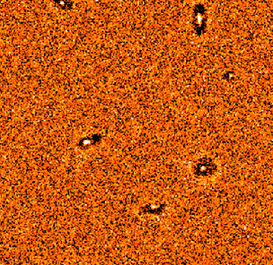
Figure 6: Typical patterns in a residual image created by t-phot, caused by inaccurate PSF/kernel determination. In this case, the ring-shaped shadow surrounding a bright central spot is due to an underestimation of the central peak of the LRI PSF, which causes an overestimation of the fit in the outskirts while leaving too much light in the centre.

ii) When dealing with extended priors, it is assumed that the instrinsic morphology of the objects does not change with the wavelength. Of course, this is usually not the case. The issue is less of a problem when dealing with FIR images, in which the morphological features of the priors are unresolved by the low-resolution PSF. On the other hand, in the optical and NIR domains this problem may be solved by the use of multicomponent analytical models as priors. In this approach, each component should be fitted independently, thus allowing the ratio between bulge and disk components to vary between the HRI and LRI. A clear drawback of this approach is that any failure of the fit due to irregular or difficult morphological features (spiral arms, blobs, asymmetries, etc.) would be propagated into the LRI solution. This functionality is already implemented in t-phot and detailed testing is ongoing.

iii) As explained in Sect. 2.2, t-phot flags priors that are likely to be flawed: sources too close to the borders of the image, saturated objects, and most notably blended priors. The assumption that all priors are well separated from one another is crucial, and the method fails when this requirement is not accomplished. Again, this is crucial only when dealing with real priors, while analytical models and unresolved priors are not affected by this limitation.

iv) As anticipated in Sect. 2.1.1, FIR images can suffer from an “overfitting” problem, due to the presence of too many priors in each LRI beam if the HRI is deeper than the LRI. In this case, a selection of the priors based on some additional criteria (e.g. flux predition from SED fitting) might be necessary to avoid catastrophic outcomes (see also Wang et al. 2015; Bourne et al. 2015, in preparation).

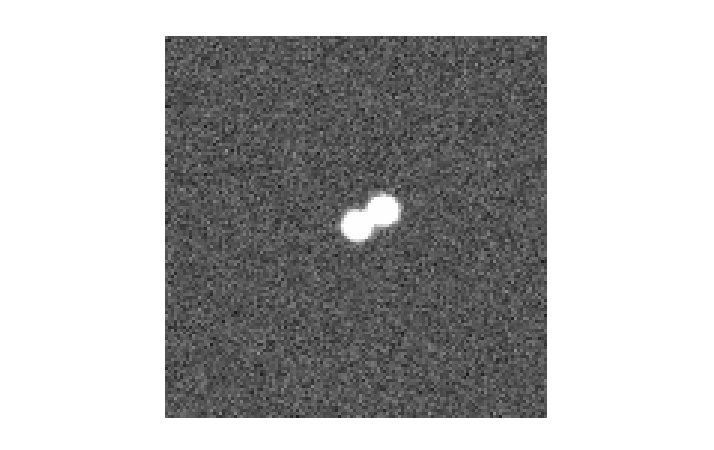
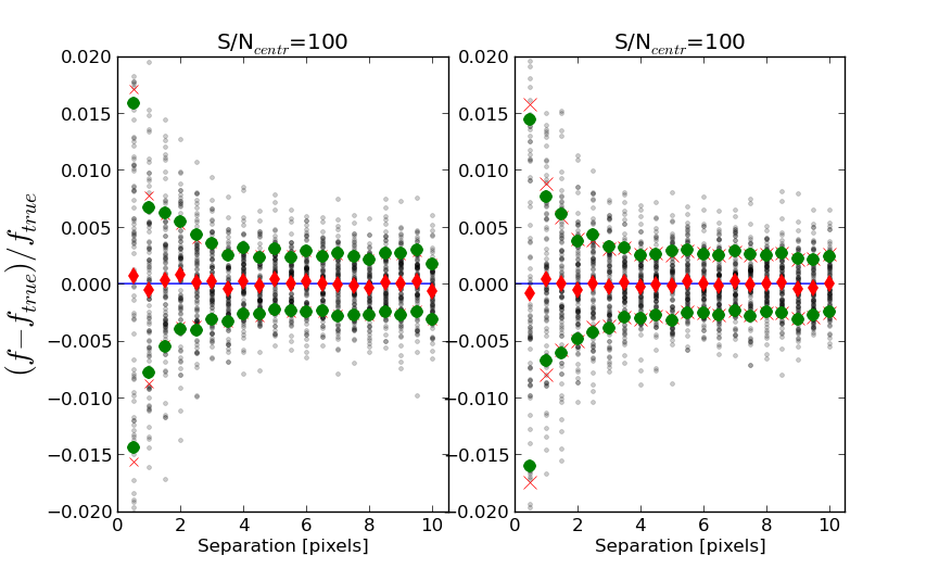
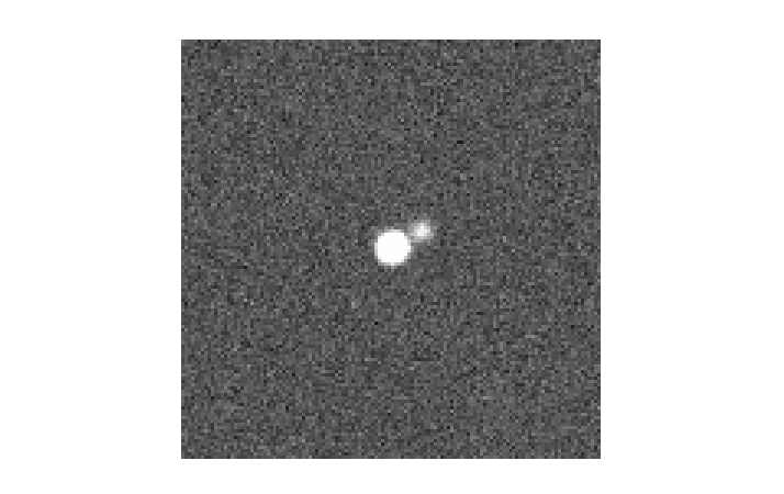
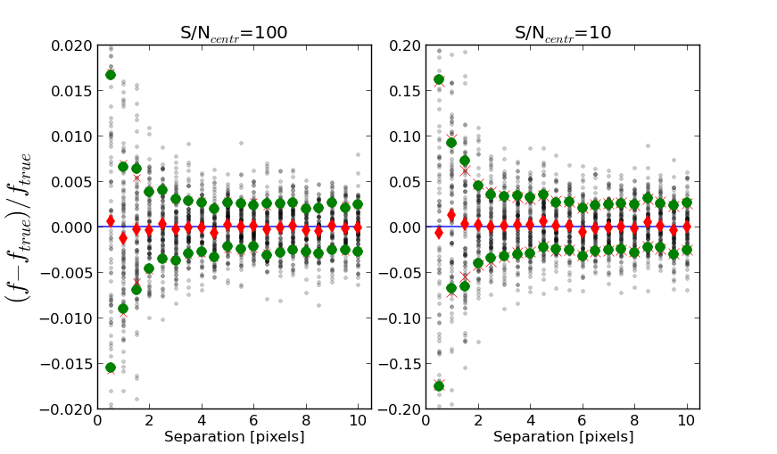
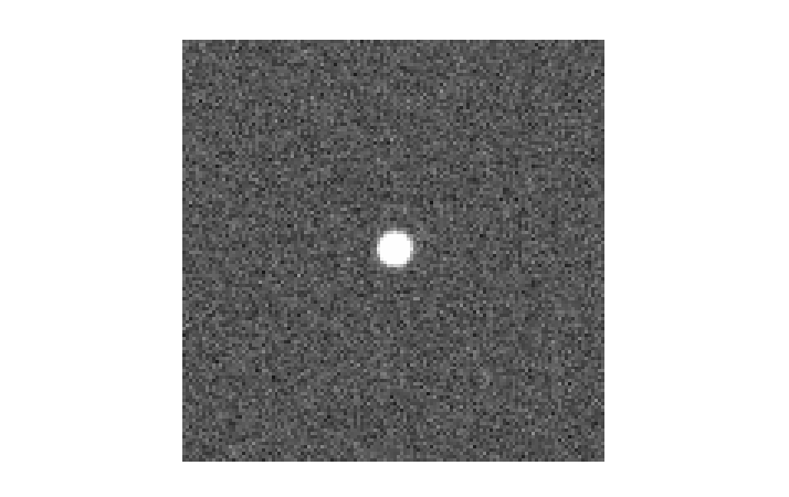
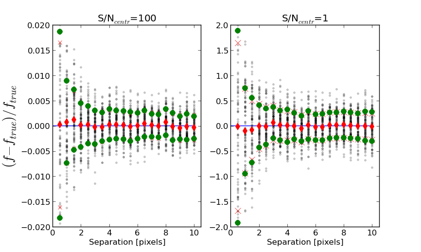
Figure 7: Accuracy check on idealized PSF-shaped objects. 100 realizations of the same image containing two PSF-shaped objects at varying positions and signal-to-noise ratios have been produced and the fluxes have been measured with t-phot. In each row, the left image shows one of the 100 realizations with the largest considered separation (10 pixels). On the right, the first panel refers to the central object, and the second (on the right) to the shifted object; central signal-to-noise ($S/N_{centr}$) ratios are, from top to bottom, 100, 100, 100 for the first source and 100, 10, 1 for the second source. In each panel, as a function of the separation interval between the two sources, the faint grey points show each of the 100 flux measurements (in relative difference with respect to the true input flux), the red diamonds are the averages of the 100 measurements, the red crosses show the nominal error given by the covariance matrix in t-phot, and the green dots the standard deviation of the 100 measurements. See text for more details.

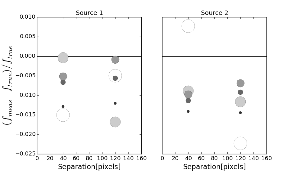
Figure 8: Effects of different segmentation areas on the measured flux of two isolated objects with identical flux and signal-to-noise ratio, at two possible separations of 40 and 120 pixels. Each panel shows the flux error in one of the objects at each separation distance. The shades and dimensions of the dots is a function of the radius of the segmentation, with darker and smaller dots corresponding to smaller segmentations. See text for more details.

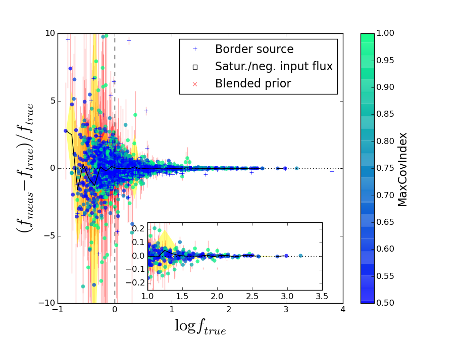
Figure 9: Accuracy of the flux determination in a simulation containing non-overlapping, PSF-shaped sources and “perfect” detection. Relative measured flux difference $(f_{meas}-f_{true})/f_{true}$ is plotted versus logarithm of the input flux $f_{true}$, for a simulated image populated with PSF-shaped sources (FWHM=1.66”). Each dot corresponds to a single source, with different symbols and colours referring to various diagnostics as explained in the legend and in the colourbar. The black solid line is the average in bins, the yellow shade is the standard deviation. The vertical dashed line shows the limiting flux at 1$\sigma$, $f=1$. The inner panel shows a magnification of the brighter end of the distribution. The fit was performed on the whole image at once. See text for more details.

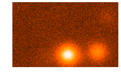
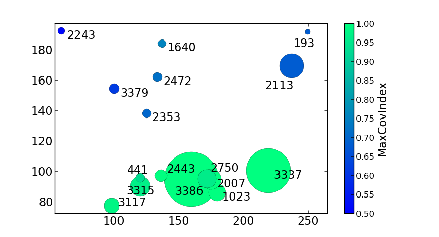
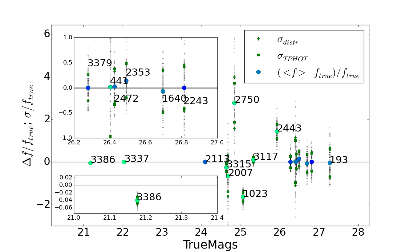
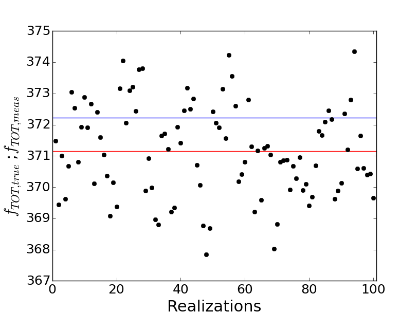
Figure 10: Analysis of a small region including a strongly covarying group of sources. Upper left panel: one of the 100 realizations with different noise maps of the region. Upper right panel: true spatial position of all the sources in the region (the colour of the dots refer to the covariance index of the sources, as indicated in the colourbar, while their size is proportional to their true flux). Bottom left panel: relative deviation of measured flux from the true flux for each source in the region, as a function of their true magnitude (big dots show the average relative deviation, and their colours refer to their covariance index as in the previous panel; green squares show the nominal uncertainty given by t-phot, to be compared with the RMS of the distribution of the 100 measurements (diamonds); small grey dots are the 100 measurements. The insets show magnifications of regions of interest). Bottom right panel: each dot shows the sum of the measured fluxes for each of the 100 realizations, and the average of this sum (red line) to be compared with the true sum (blue line), showing that an overall consistency is guaranteed by the method. See text for more details.

4 Validation

To assess the performance of t-phot we set up an extensive set of simulations, aimed at various different and complementary goals.

We used SkyMaker (Bertin 2009), a public software tool, to build synthetic .fits images. The code ensures direct control on all the observational parameters (the magnitude and positions of the objects, their morphology, the zero point magnitude, the noise level, and the PSF). Model galaxies were built by summing a de Vaucouleurs and an exponential light profile in order to best mimic a realistic distribution of galaxy morphologies. These models were generated using a variety of bulge-to-total light ratios, component sizes, and projection angles.

All tests were run using ideal (i.e. synthetic and symmetric) PSFs and kernels.

Moreover, we also performed tests on real datasets taken from the CANDELS survey (in these cases using real PSFs).

Some of the tests were performed using both t-phot and tfit, to cross-check the results, ensuring the perfect equivalency of the results given by the two codes when used with the same parameter sets, and showing how appropriate settings of the t-phot parameters can ensure remarkable improvements.

For simplicity, here we only show the results from a restricted selection of the test dataset, which are representative of the performance of t-phot in standard situations. The results of the other simulations resemble overall the ones we present, and are omitted for the sake of conciseness.

4.1 Code performance and reliability on simulated images

4.1.1 Basic tests

As a first test, we checked the performance of the basic method by measuring the flux of two PSF-shaped synthetic sources, with varying separation and signal-to-noise ratios. One hundred realizations with different noise maps of each parameter set were prepared, and the averages on the measured fluxes were computed. The aims of this test were twofold: on the one hand, to check the precision to which the fitting method can retrieve true fluxes in the simplest possible case - two sources with ideal PSF shape; on the other hand, to check the reliability of the nominal error budget given by the covariance matrix, comparing it to the real RMS of the 100 measurements. Figure 7 shows three examples of the set-up and the results of this test. Clearly, in both aspects the results are reassuring: the average of the 100 measurements (red diamonds) is always in very good agreement with the true value, with offset in relative error always well under the $1/(S/N)_{centr}$ limit ($(S/N)_{centr}$ is the value of the signal-to-noise ratio in the central pixel of the source, corresponding to roughly one third of the total $S/N$); and the nominal error (red crosses) given by the covariance matrix is always in good agreement with the RMS of the 100 measurements (red circles).

When dealing with extended objects rather than with point-like sources, one must consider the additional problem that the entire profile of the source cannot be measured exactly because the segmentation is limited by the lowest signal-to-noise isophote. The extension of the segmentation therefore plays a crucial role and defining it correctly is a very subtle problem. Simply taking the isophotal area as reported by SExtractor as ISOAREA often underestimates the real extension of the objects. Accordingly, the segmentation of the sources should somehow be enlarged to include the faint wings of sources. To this aim, specific software called Dilate was developed at OAR and used in the CANDELS pipeline for the photometric analysis of GOODS-S and UDS IRAC data (Galametz et al. 2013). Dilate enlarges the segmentation by a given factor, depending on the original area; it has proven to be reasonably robust in minimizing the effects of underestimated segmentated areas.

Figure 8 shows the effects of artificially varying the dimensions of the segmentation relative to two bright, extended and isolated sources in a simulated HRI, on the flux measured for that source in a companion simulated LRI. It is important to note how enlarging the segmented area normally results in larger measured fluxes, because more and more light from the faint wings of the source are included in the fit. However, beyond a certain limit the measurements begin to lose accuracy owing to the inclusion of noisy, too low signal-to-noise regions (which may cause a lower flux measurement).

In principle, using extended analytical models rather than real high-resolution cutouts should cure this problem more efficiently, because models have extended wings that are not signal-to-noise limited. Tests are ongoing to check the performance of this approach, and will be presented in a forthcoming paper.

4.1.2 Tests on realistic simulations

The next tests were aimed at investigating less idealized situations, and have been designed to provide a robust analysis of the performance of the code on realistic datasets. We used the code GenCat (Schreiber et al. 2015, in preparation) to produce mock catalogues of synthetic extragalactic sources, with reasonable morphological features and flux distribution. Then, a set of images were produced using such catalogues as an input for SkyMaker. A “detection” HRI mimicking an HST H band observation (FWHM = $0.2^{\prime\prime}$) was generated from the GenCat catalogue using output parameters to characterize the objects’ extended properties. Then a set of measure LRIs were produced: the first was populated with PSF-shaped sources, having FWHM = 1.66” (the typical IRAC-ch1/ch2 resolution, a key application for t-phot), while other LRIs were created from the input catalogue, mimicking different ground-based or IRAC FWHMs. Finally, we created another HRI catalogue removing all of the overlapping sources. This “non-overlapping” catalogue was used to create parallel detection and measurement images in order to obtain insight into the complications given by the presence of overlapping priors. In all these images, the limiting magnitude was set equal to the assigned zero point, so that the limiting flux at 1$\sigma$ is 1. In addition, the fits were always performed on the LRI as a whole, if not otherwise specified.

Figure 9 shows the results relative to the first test, i.e. the fit on the image containing non-overlapping, PSF-shaped sources, with a “perfect” detection (i.e. the priors catalogue contains all sources above the detection limit), obtained with a single fit on the whole image. The figure shows the relative error in the measured flux of the sources, $(f_{meas}-f_{true})/f_{true}$, versus the log of the real input flux $f_{true}$; the different symbols refer to the flag assigned to each object, while the colour is a proxy for the covariance index.

In this case, the only source of uncertainty in the measurement is given by the noise fluctuations, which clearly become dominant at the faint end of the distribution. Looking at the error bars of the sources, which are given by the nominal error assigned by t-phot from the covariance matrix, one can see that almost all sources have measured flux within $2\sigma$ from their true flux, with only strongly covariant sources (covariance index $\simeq$ 1, greener colours) having $|f_{meas}-f_{true}|/f_{true}>1\sigma$. The only noticeable exceptions are sources that have been flagged as potentially unreliable, as described in Sect. 2.2. We also note how the average $\Delta f/f$ (solid black line) is consistent with zero down to $f_{true}=S/N\simeq 0.63$.

Figure 10 shows the analysis of a case study in which the fluxes of a clump of highly covariant objects are measured with poor accuracy, and some of the nominal uncertainties are underestimated: a very bright source (ID 3386, m${}_{true}=21.17$) shows a relative difference $(f_{meas}-f_{true})/f_{true}>3\sigma$. To cast light on the reason for such a discrepancy, the region surrounding the object was replicated 100 times with different noise realizations, and the results were analysed and compared. The upper panels show (left) one of the 100 measurement images and (right) the position of all the sources in the region (many of which are close to the detection limit). The colour code refers to the covariance index of the sources. The bottom left panel shows the relative error in the measured flux for all the sources in the region, with the inner panels showing magnifications relative to the object ID 3386 and to the bunch of objects with m${}_{true}\sim 26.5$. Looking at the colours of their symbols, many objects in the region turn out to be strongly covariant. Indeed, while the bluer sources in the upper part of the region all have covariant indexes lower than 0.5, the greener ones in the crowded lower part all have covariance index larger than 1 (indeed larger than 2 in many cases). This means that their flux measurements are subject to uncertainties not only from noise fluctuations, but also from systematic errors due to their extremely close and bright neighbours. As clearly demonstrated here, the covariance index can give a clue to which measurements can be safely trusted.

The bottom right panel gives the sum of the measured fluxes of all sources in each of the 100 realizations (the blue line is the true total flux and the red line is the mean of the 100 measured total fluxes). It can be seen that the total flux measured in the region is always consistent with the expected true one to within $\simeq 1\%$ of its value.

Although it is not possible to postulate a one-to-one relation (because in most cases sources having a large covariance index have a relatively good flux estimate, see Fig. 9), the bottom line of this analysis is that the covariance index, together with the flagging code outputted by t-phot, can give clues about the reliability of measured flux, and should be taken into consideration during the analysis of the data. Measurements relative to sources having a covariance index larger than 1 should be treated with caution.

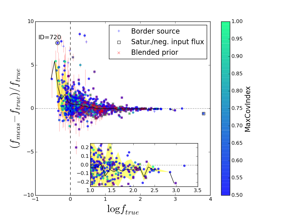
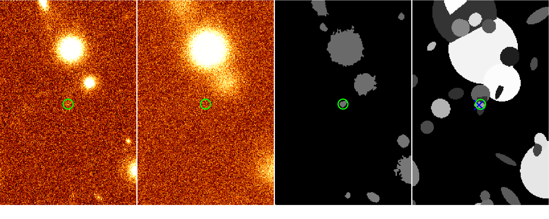
Figure 11: Accuracy of the flux determination in a simulation containing extended objects, overlapping priors, and SExtractor detection. Top: relative flux difference $(f_{meas}-f_{true})/f_{true}$ versus logarithm of the input flux $f_{true}$ for a simulated image populated with extended sources (FWHM=1.66”). Symbols and colours are as in Fig. 9. The inner panel shows a magnification of the brighter end of the distribution. The outlier marked with the open black circle, ID=720, is shown in the bottom panel: left to right, HRI (FWHM=0.2”), LRI, SExtractor segmentation map and “true” segmentation map. The green circles show the object detected via SExtractor, while the blue cross shows its “true” position. See text for more details.

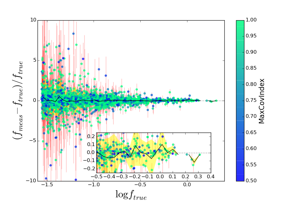
Figure 12: Accuracy of the flux determination in a FIR-like simulation (Herschel SPIRE 250 $\mu$m, FWHM=25”, 3.6” pixel scale), using unresolved priors. The symbols have the same meaning as in Fig. 11. See text for more details.

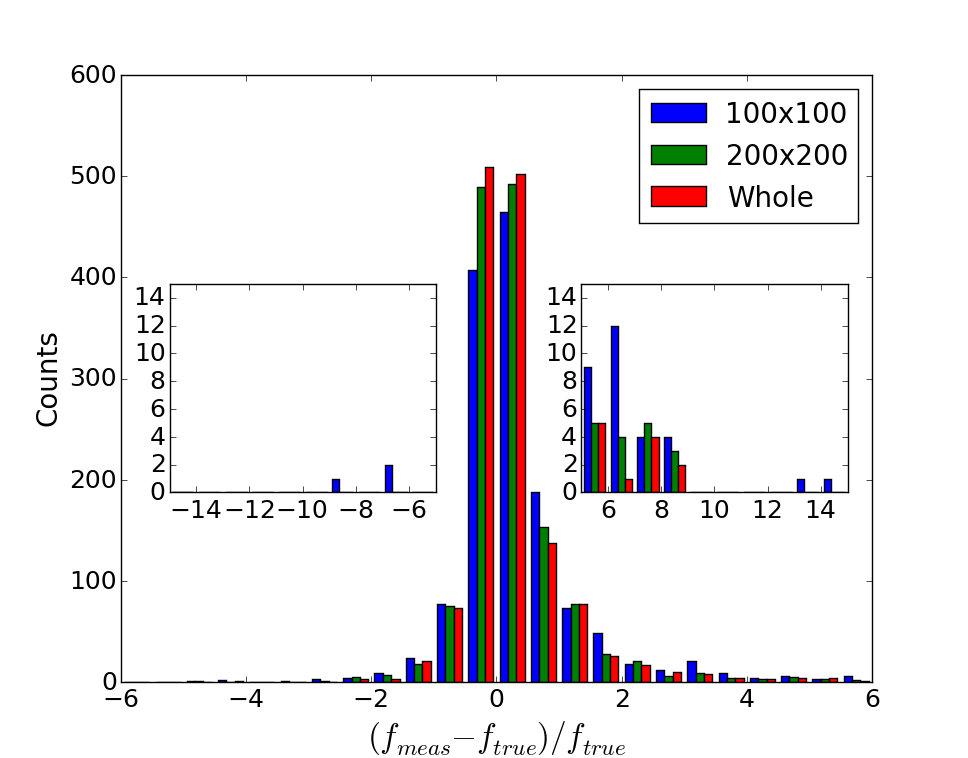
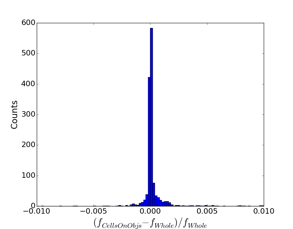
Figure 13: Accuracy of the flux determination. Top panel: for the same simulation described in Fig. 11, the histograms show the results for three different fitting methods: regular grid 100$\times$100 pixels (standard tfit approach), regular grid 200$\times$200, single fit on the whole image. The small boxes show the extended wings of the histograms, magnified for better viewing. The accuracy increases by enlarging the cells and, reaches the best result with the single fit on the whole image. Bottom panel: the histogram shows the relative measured flux difference between the single fit on the whole image and the cells-on-objects method. Differences above $1\%$ are very rare.

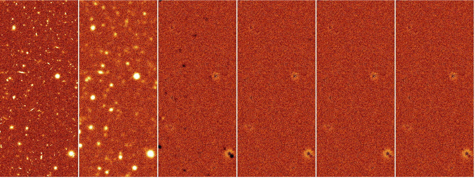
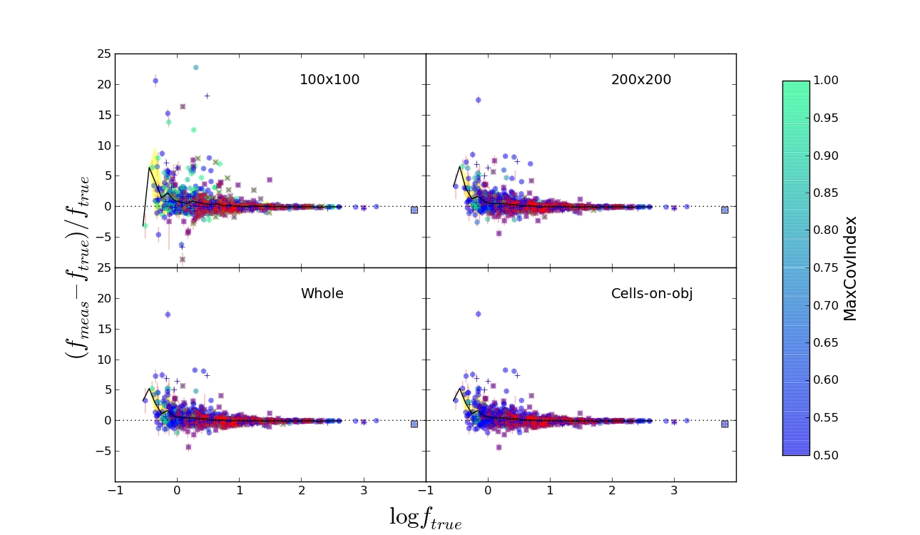
Figure 14: Accuracy of the flux determination. For the same simulation described in Fig. 11, the plots show the results for four different fitting methods. Top panel, left to right: HRI (FWHM=0.2”), LRI (FWHM=1.66”), residuals using a regular grid of $100\times 100$ pixels cells (standard tfit approach), a regular grid of $200\times 200$ pixels cells, a single fit on the whole image, and the cells-on-objects method. The spurious fluctuations in the last two panels are due to segmentation inaccuracies, as in Fig. 11. Bottom panels, left to right and top to bottom: relative measured flux differences with respect to true fluxes, same order as above. The values of the covariance index are different in each case because of the varying sizes of the cells (and therefore of the relative matrix).

In a subsequent more realistic test, we considered extended objects (including morphologies of objects from the GenCat catalogue, using FWHM_HRI=0.2” and FWHM_LRI=1.66” and imposing m_true,LRI=m${}_{true,HRI}=m_{H160,GenCat}$ for simplicity) and allowed for overlapping priors. To be consistent with the standard procedure adopted for real images, for this case we proceeded by producing an SExtractor catalogue and segmentation map, which were then spatially cross-correlated with the “true” input catalogue. The results for this test are shown in Fig. 11. Even in this much more complex situation, the results are reassuring; there is an overall good agreement between measured and input fluxes for bright ($\log S/N>1$) sources, with only a few flagged objects clearly showing large deviations from the expected value, and a reasonably good average agreement down to $\log S/N=0$. However, all bright fluxes are measured $\simeq 5\%$ fainter than the true values (see the inner box in the same figure); this is very likely the effect of the limited segmentation extension, as already discussed in the previous section. On the other hand, faint sources tend to have systematically overestimated fluxes, arguably because of contamination from undetected sources. To confirm this, we focus our attention on a single case study (the source marked as ID 720) which shows a large discrepancy from its true flux, but has a relatively small covariance index. An analysis of the real segmentation map shows how the detected object is actually a superposition of two different sources that have been detected as a single one, so that the measured flux is of course higher than expected. One should also note that the uncertainties on the measured fluxes are smaller in this test, because there are fewer priors (only the ones detected by SExtractor are now present), implying a lower rank of the covariance matrix and a lower number of detected neighbours blending in the LRI. This causes a global underestimation of the errors.

To check the performance of t-phot at FIR wavelengths, we also run a test on a simulated Herschel SPIRE 250 $\mu$m image (FWHM=25”, 3.6” pixel scale). The simulated image (shown alongside with the obtained residuals in Fig. 4) mimics real images from the GOODS-Herschel program, the deepest Herschel images ever obtained. This image was produced with the technique presented in Leiton et al. (2015); we first derived (predicted) flux densities for all the 24 $\mu$m detections ($F_{24\mu m}>20\mu$Jy) in GOODS-North, which are dependent on their redshift and flux densities at shorter wavelengths, and then we injected these sources into the real noise maps from GOODS-Herschel imaging. Additional positional uncertainties, typically 0.5$\arcsec$, were also applied to mimic real images. As shown in Leiton et al. (2015), these simulated images have similar pixel value distributions to real images (see also Wang et al. 2015, for more details). For this test, t-phot was run using the list of all the 24 $\mu$m sources as unresolved priors. The results of the test are plotted in Fig. 12, and they show that even in this case t-phot can recover the input fluxes of the sources with great statistical accuracy (the mean of the relative deviation from the expected measurements, i.e. the black solid line in the plot, is consistent with zero down to the faintest fluxes). The results are equivalent to those obtained on the same datasets with other public software specifically developed for FIR photometry, such as FastPhot (Béthermin et al. 2010).

4.1.3 Testing different fitting options: cell dimensions

We then proceeded to check the performance of the different fitting techniques that can be used in t-phot. To this aim, we repeated the test on the 1.66” LRI with extended priors and SExtractor priors, described in Sect. 4.1.2, with different fitting methods: using a regular grid of cells of $100\times 100$ pixels, a regular grid of cells of $200\times 200$ pixels, and the cells-on-objects method, comparing the results with those from the fit of the whole image at once. The results of the tests are shown in Figs. 13 and 14. The first figure compares the distributions of the relative errors in measured flux for the runs performed on the $100\times 100$ pixels grid, on the $200\times 200$ pixels grid, and on the whole image at once. Clearly, using any regular grid of cells worsens the results, as anticipated in Sect. 2.1.5. Enlarging the sizes of the cells improves the situation, but does not completely solve the problem. We note that the adoption of an arbitary grid of cells of any dimension in principle is prone to the introduction of potentially large errors, because (possibly bright) contaminating objects may contribute to the brightness measured in the cell, without being included as contributing sources. A mathematical sketch of this issue is explained in the Appendix B (see also Sect. 4.2). The second histogram compares the differences between the fit on the whole image and the fit with the cells-on-objects method. Almost all the sources yield identical results with the two methods, within $(f_{meas}-f_{true})/f_{true}<0.001$, which proves that the cells-on-objects method can be considered a reliable alternative to the single-fit method. Finally, Figure 14 compares the HRI, the LRI, and the residual images obtained with the four methods and their distributions of relative errors, showing quantitatively the difference between the analyzed cases.

In summary, it is clear that an incautious choice of cell size may lead to unsatisfactory and catastrophic outcomes. On the other hand, the advantages of using a single fit, and the equivalence of the results obtained with the single-fit and the cells-on-objects techniques, are evident. As already anticipated, one should bear in mind that the cells-on-objects method is only convenient if the overlapping of sources is not dramatic, as in ground-based optical observations. For IRAC and FIR images, on the other hand, the extreme blending of sources would cause the cells to be extended over regions approaching the size of the whole image, so that a single fit would be more convenient, although often still CPU-time consuming.

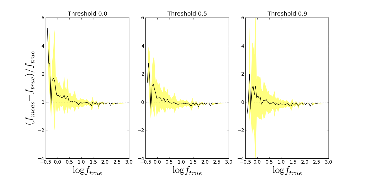
Figure 15: Effects of threshold fitting (Sect. 4.1.4). Mean relative error (black line) and standard deviation (yellow shaded area) for three simulations with different threshold values (0.0, 0.5, 0.9). Only pixels with normalized flux higher than the threshold values are included in the fit. Larger threshold values result in more accurate measurements for faint sources, at the expense of a systematic underestimation of the flux for brighter ones.

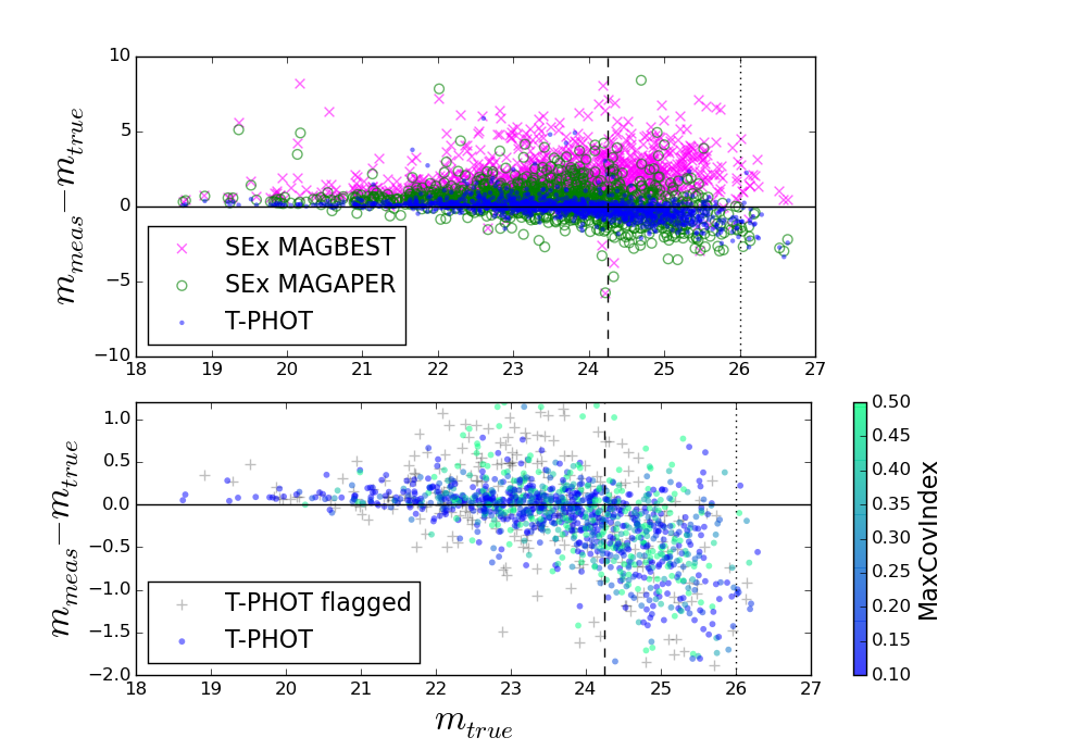
Figure 16: Top: measured magnitude differences $(m_{meas}-m_{true})$ versus “true” input magnitudes $m_{true}$, for two simulated images populated with extended sources (HRI has FWHM=0.2” and HST $H$band-like fluxes, LRI has FWHM=1.66” and IRACch1-like fluxes), using three different methods: SExtractor dual-mode aperture, SExtractor dual-mode “best”, and t-phot. Vertical lines show the $5\sigma$ (dashed) and $1\sigma$ (dotted) limits of the simulated LRI. Bottom: magnification of the top panel, showing only t-phot results, colour-coded as a function of the covariance index. See text for more details.

4.1.4 Testing different fitting options: threshold fitting

As described in Sect. 2.1.5, t-phot includes the option of imposing a lower threshold on the normalized fluxes of templates so as to exclude low signal-to-noise pixels from the fit. Figure 15 shows a comparison of the relative errors obtained with three different values of the THRESHOLD parameter: $t=0$, $t=0.5$, and $t=0.9$ (whic means that only pixels with normalized flux $f_{norm}>t\times f_{peak}$ in the convolved template will be used in the fitting procedure). The differences are quite small; however, a non-negligible global effect can be noticed: all sources tend to slightly decrease their measurement of flux when using a threshold limit. This brings faint sources (generally overestimated without using the threshold) closer to their true value, at the same time making bright sources too faint. This effect deserves careful investigation, which is beyond the scope of this study, and is postponed to a future paper.

4.1.5 Colours

A final test was run introducing realistic colours, i.e. assigning fluxes to the sources in the LRI consistent with a realistic SED (as output by GenCat, see Sect. 4.1.2), instead of imposing them to be equal to the HRI fluxes. We took IRAC-ch1 as a reference filter for the LRI, consistently with the chosen FWHM of 1.66”. Furthermore, we allowed for variations in the bulge-to-disc ratios of the sources to take possible effects of colour gradients into account. We compared the results obtained with t-phot with the ones obtained with two alternative methods to determine the magnitudes of the sources in the LRI: namely, SExtractor dual mode aperture and MAG_BEST photometry (with HRI as detection image). The differences between measured and input magnitudes in the LRI, m${}_{meas}-$m_true, are plotted in Fig. 16. Clearly, t-phot ensures the best results, with much less scatter in the measurements than both of the other two methods, and very few outliers.

4.2 Performance on real datasets

It is instructive to check how t-phot performs on real datasets, in addition to simulations. To this aim, we run two different tests. In the first, we compared the results of the tfit CANDELS analysis on the UDS CANDELS $I$-band (Galametz et al. 2013) to a t-phot run obtained using the cells-on-objects method and different parameters in the kernel registration stage. Figure 18 shows the histograms of the differences in the photometric measurements between tfit and t-phot. Many sources end up with a substantially different flux, because of the two cited factors (a better kernel registration and the different fitting procedure). We note that the majority of the sources have fainter fluxes with respect to the previous measurements, precisely because of the effect described in Sect. 4.1.2: fitting using a grid of cells introduces systematic errors assigning light from sources that are not listed in a given cell, but overlap with it to the objects recognized as belonging to the cell. To further check this point, Fig. 19 shows some examples of the difference between the residuals obtained with tfit (official catalogue) and those obtained with this t-phot run using cells-on-objects method, also introducing better registration parameters in the dance stage. Clearly, the results are substantially different, and many black spots (sources with spurious overestimated fluxes) have disappeared. Also, the registrations appear to be generally improved.

The second test was run on FIR/sub-mm SCUBA-2 (450 $\mu$m, FWHM=7.5”) and Herschel (500 $\mu$m, FWHM=36”) images of the COSMOS-CANDELS field. In both cases, a list of 24+850 $\mu$m sources was used as unresolved priors. Figure 17 shows the original images in the top row, and the residuals in the bottom row. The model has removed all significant sources from the 450 $\mu$m map and the majority from the 500 $\mu$m map. Figure 20 shows a comparison of the fluxes measured in the t-phot fits to the 450 $\mu$m and 500 $\mu$m maps at 24+850 $\mu$m prior positions, with the error bars combining the errors on both flux measurements. Agreement within the errors implies successful deconfusion of the Herschel image to reproduce the fluxes measured in the higher resolution SCUBA-2 image. This typology of analysis is very complex and we do not want to address here the subtleties of the process; we refer the reader to Wang et al. (2015, in preparation) and Bourne et al. (2015, in preparation) for detailed discussions on the definition of a robust and reliable approach to measure FIR and sub-mm fluxes. These simple tests, however, clearly show that t-phot is successful at recovering the fluxes of target sources even in cases of extreme confusion and blending, within the accuracy limits of the method.

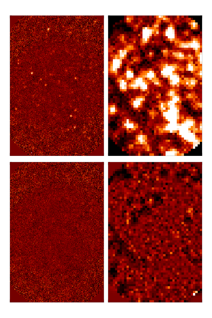
Figure 17: Results from a test run using t-phot with unresolved priors on FIR/sub-mm real dataset. Upper row, left to right: SCUBA-2 450 $\mu$m (FWHM=7.5”) and Herschel 500 $\mu$m (FWHM=36”) images of the COSMOS-CANDELS fields. Lower row, left to right: residuals for the two fields, obtained with t-phot runs using a list of 24+850 $\mu$m priors. See text for details.

5 Computational times

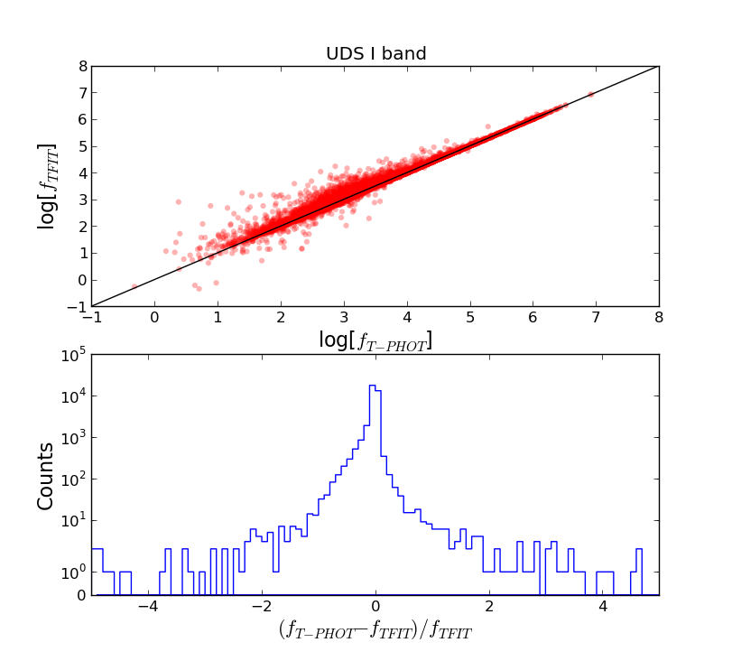
Figure 18: UDS I band tfit versus t-phot comparison. Top panel: compared measured fluxes. Bottom panel: histogram of relative measured flux difference.

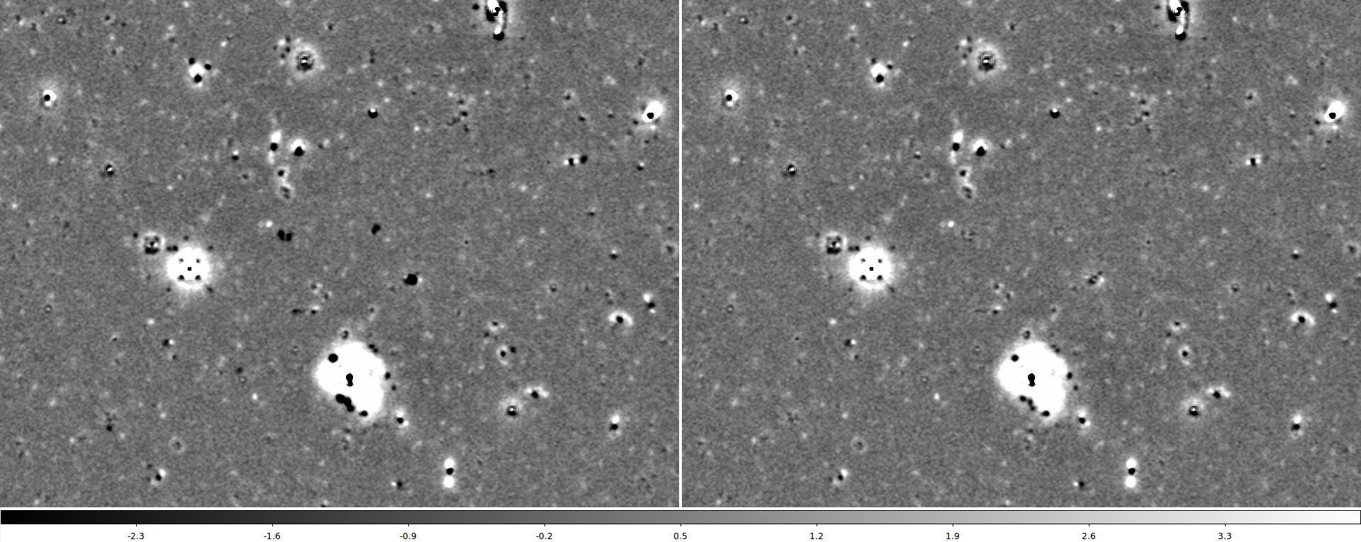
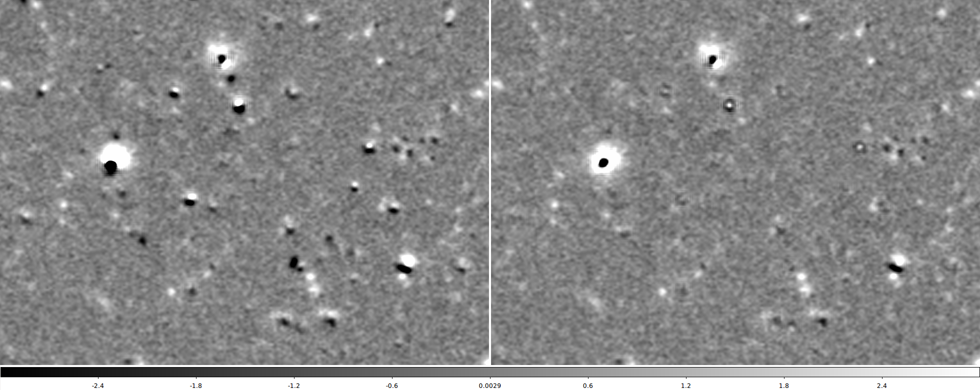
Figure 19: UDS I band tfit versus t-phot comparison. The panels on the left show two small patches of the official CANDELS residual image obtained using t-fit. The residual images of the same regions are showed in the right panels, this time obtained using t-phot with cells-on-objects method and improved local kernel registration. We note the disappearence of many spurious black spots.

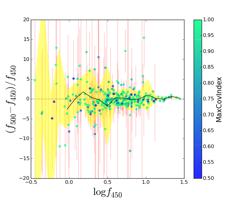
Figure 20: Accuracy of the flux determination for the dataset described in Fig. 17: measured Herschel 500 $\mu$m (FWHM=36”) fluxes $f_{500}$ are compared to the fluxes obtained for the SCUBA-2 450 $\mu$m (FWHM=7.5”) $f_{450}$, considered as reference fluxes (using 24+850 $\mu$m unresolved priors in both cases). The symbols have the same meaning as in Fig. 11; the error bars now include the measured error on the reference flux. See text for more details.

As anticipated, t-phot ensures a large saving of computational time compared to similar codes like tfit and convphot when used with identical input parameters. For example, a complete, double-pass run on the whole CANDELS UDS field at once (I band; $\sim$35000 prior sources; LRI 30720$\times$12800 $\simeq$ 400 million pixels; standard tfit parameters and grid fitting) is completed without memory swaps in about 2 hours (i.e. 1 hour per pass) on a standard workstation (Intel i5, 3.20 GHz, RAM 8 Gb). A complete, double-pass run on the GOODS-S Hawk-I W1 field ($\sim$17500 prior sources, LRI 10700$\times$10600 $\simeq$ 100 millions pixels, identical parameters) is completed in $\sim$20 minutes. For comparison, tfit may require many hours ($\sim$24) to complete a single pass on this Hawk-I field on the same machine. It must be said that tfit by default produces cutouts and templates for all the sources in the HRI image; selecting the ones belonging to the LRI field and inputting an ad hoc catalogue would have reduced the computing time by a factor of two (i.e. 11 hours for a single pass). It was not possible to process large images like the UDS field in a single run, because of RAM memory failure. convphot timings and memory problems are similar to those of tfit, although they have different causes (being written in C, computation is generally faster, but it employs a slower convolution method and the solution of the linear system in performed as a single fit instead of grid fitting like in tfit, being much more time consuming).

Adopting the cells-on-objects (Sect. 2.1.5) method increases the computational time with respect to the tfit standard cell approach, but it is still far more convenient than the convphot standard single-fit approach, and gives nearly identical results.

Table 2 summarizes the computational times for extended tests on a set of simulated images having different detection depths (and therefore number of sources) and dimensions, with LRI FWHM=1.66”. The simulations were run on the same machine described above, using three different methods: whole image fitting, cells-on-objects, and $100\times 100$ pixels cells fitting.

	27	28	29
Number of sources
$2500\times 2500$	523	1070	1398
$5000\times 5000$	2104	4237	5561
$10000\times 10000$	8390	16807	22394
$20000\times 20000$	33853	65536	65536
Whole image fitting
$2500\times 2500$	38” (2”)	54” (10”)	1’9” (20”)
$5000\times 5000$	3’26” (1’1”)	11’9” (7’41”)	20’28” (16’1”)
$10000\times 10000$	1h28’22” (1h15’46”)	8h26’1” (7h58’10”)	21h16’24” (20h27’53”)
$20000\times 20000$	-	-	-
Cells-on-objects fitting
$2500\times 2500$	46” (4”)	1’11” (16”)	1’30” (33”)
$5000\times 5000$	3’1” (18”)	4’27” (1’8”)	6’3” (2’20”)
$10000\times 10000$	12’27” (1’12”)	17’52” (4’31”)	25’11” (9’52”)
$20000\times 20000$	51’12” (6’1”)	1h34’40” (35’8”)	1h43’10” (41’2”)
100$\times$100 pixels cells fitting
$2500\times 2500$	52” (3”)	1’6” (7”)	1’14” (9”)
$5000\times 5000$	3’16” (14”)	4’22” (29”)	4’54” (41”)
$10000\times 10000$	13’4” (56”)	17’12” (1’54”)	19’47” (2’53”)
$20000\times 20000$	55’24” (6’19”)	1h18’38” (15’53”)	1h17’17” (17’58”)

Table 2: Test of computational times for t-phot runs on images of given dimensions and limiting magnitude in detection. Each entry of the table gives the total duration of run, the duration the fitting stage alone (in parentheses), and the number of fitted sources. The dance stage takes most of the CPU time after the fitting routine.

6 Summary and conclusions

We have presented t-phot, a new software package developed within the astrodeep project. t-phot is a robust and versatile tool, aimed at the photometric analysis of deep extragalactic fields at different wavelengths and spatial resolution, deconfusing blended sources in low-resolution images.

t-phot uses priors obtained from a high-resolution detection image to obtain normalized templates at the lower resolution of a measurement image, and minimizes a $\chi^{2}$ problem to retrieve the multiplicative factor relative to each source, which is the searched quantity, i.e. the flux in the LRI. The priors can be either real cutouts from the HRI, or a list of positions to be fitted as PSF-shaped sources, or analytical 2-D models, or a mix of the three types. Different options for the fitting stage are given, including a cells-on-objects method, which is computationally efficient while yielding accurate results for relatively small FWHMs. t-phot ensures a large saving of computational time as well as increased robustness with respect to similar public codes like its direct predecessors tfit and convphot. With an appropriate choice of the parameter settings, greater accuracy is also achieved.

As a final remark, it should be pointed out that the analysis presented in this work deals with idealized situations, namely simulations or comparisons with the performances of other codes on real datasets. There are a number of subtle issues regarding complex aspects of the PSF-matching techinque, which become of crucial importance when working on real data. A simple foretaste of such complexity can be obtained by considering the problem described in Sect. 4, i.e. the correct amplitude to be assigned to the segmented area of a source. Work on this is ongoing, and the full discussion will be presented in a subsequent companion paper.

As we have shown, t-phot is an efficient tool for the photometric measurements of images on a very broad range of wavelengths, from UV to sub-mm, and is currently being routinely used by the Astrodeep community to analyse data from different surveys (e.g. CANDELS, Frontier Fields, AEGIS). Its main advantages with respect to similar codes like tfit or convphot can be summarized as follows:

• when used with the same parameter settings of tfit, t-phot is many times faster (up to hundreds of times), and the same can be said with respect to other similar codes (e.g., convphot);

• t-phot is more robust, more user-friendly, and can handle larger datasets thanks to an appropriate usage of the RAM;

• t-phot can be used with three different types of priors (real high-resolution cutouts, analytical models and/or unresolved point sources) making it a versatile tool for the analysis of different datasets over a wide range of wavelengths from UV to sub-mm;

• t-phot offers many options for performing the fit in different ways, and with an appropriate choice of parameter settings it can give more accurate results.

Future applications might include the processing of EUCLID and CCAT data. New releases of the software package, including further improvements and additional options, are planned for the near future.

Appendix A The parameter file

Below is a template of the standard first-pass parameter file to be given as input to t-phot (similar templates for both the first and the second pass are included in the dowloadable tarball). It is very similar to the original tfit parameter file, and part of the description is directly inherited from it.

# T-PHOT PARAMETER FILE

# PIPELINE

# 1st pass
order standard
#priors, convolve, fit, diags, dance, plotdance

# PRIORS STAGE

# Choose priors types in use:
userealΨ ΨTrue
usemodelsΨTrue
useunresolvedΨTrue

# Real 2-d profiles
hiresfile       HRI.fits
hirescat        HRI.catΨ
hiresseg        HRI.seg.fits
normalize       trueΨ
subbckgΨΨTrue
savecutΨΨtrueΨ
cutoutdir       cutoutsΨ
cutoutcat       cutouts/_cutouts.cat

# Analytical 2-d models
modelscatΨmodels/models.cat
modelsdirΨmodelsΨΨ

cullingΨΨfalse

# Unresolved point-like sources
poscatΨΨpos.cat
psffile Ψpsf.fits

# CONVOLUTION STAGE

loresfile       LRI.fits
loreserr        LRI.rms.fits
errtype         rms
rmsconstant     1
relscale        1

FFTconvΨΨtrue
multikernelsΨfalseΨ
kernelfile      kernel.fits
kernellookup    ch1_dancecard.txt

templatedir     templates
templatecatΨtemplates/_templates.cat

# FITTING STAGE

# Filenames:
fitparsΨ         tpipe_tphot.param
tphotcat         lores_tphot.cat_pass1
tphotcell        lores_tphot.cell_pass1
tphotcovar       lores_tphot.covar_pass1

# Control parameters:
fittingΨΨcoo
cellmask        true
maskfloor       1e-9
writecovar      true

thresholdΨ0.0
linsyssolverΨlu
clipΨΨfalse

# DIAGNOSTICS STAGES

modelfile       lores_collage_pass1.fits

# Dance:Ψ
dzonesize       100
maxshift        1.0
ddiagfile       ddiags.txt
dlogfile        dlog.txt
dancefftΨfalse

A.1 Pipeline

Standard optical/NIR double-pass runs can be achieved by setting order standard and order standard2.

A standard first-pass run includes the stages priors, convolve, fit, diags, dance, plotdance. The stage priors allows for an automatic re-construction of the pipeline depending on the input data given in the following sections (see the documentation included in the tarball). A standard second-pass run includes the stages convolve, fit, diags, archive. The archive stage creates a directory after the name of the LRI, with some specifications, and archives the products of both runs.

Double-pass runs for FIR/sub-mm can be achieved by setting order positions, fit, diags, dance, plotdance and order positions, fit, diags, archive.

A.2 Priors

Each prior must have a unique identification number (ID) to avoid errors. The user must be careful to give the correct information in this paramfile. Select the priors to be used by switching on/off the relative keywords: usereal, usemodels, useunresolved.

• hiresfile: the high-resolution, detection image. If a catalogue and a segmentation map are given in the two subsequent entries (hirescat and hiresseg), cutouts will be created out of this image. This step is necessary if a catalogue of real or model priors are to be used. The catalogue hirescat must be in a standard format: id x y xmin ymin xmax ymax background SEx_flux (x and y are the coordinates of the source in HRI pixel reference frame; xmin, ymin, xmax, ymax are the limits of the segmentation relative to the source in HRI pixel reference frame; background is the value of the local background; and SEx_flux is a reference isophotal flux).

• poscat: a catalogue of positions for unresolved, point-like sources. No HRI image/segmentation is needed, while the PSF to be used to create the models is mandatory (psffile). The catalogue must be in the standard format id x y.

• modelscat: a catalogue (with format id x y xmin ymin xmax ymax background SEx_flux, as for a standard HRI priors catalogue) of model priors. modelsdir is the directory in which the stamps of the models are stored. Models with two or more components can be processed, but each component must be treated as a separated object, with a different ID, and a catalogue for each component must be given. Catalogues for each component must have the same name, but ending with ”_1”, ”_2”, etc.; put the ”_1” catalogue in the paramfile. It is important to note that two components of the same object should not have exactly identical positions, to avoid numerical divergencies.

• culling: if True, objects in the catalogue (real priors and/or models) but not falling into the LRI frame will not be processed; if it is false, all objects in the catalogue will be processed (useful for storing cutouts for future reuse on different datasets) and the selection of objects will be done before the convolution stage.

• subbckg: if True, subtract the value given in the input catalogue from each cutout stamp.

• cutoutdir: the directory containing the cutouts.

• cutoutcat: the catalogue of the cutouts, containing the flux measured within the cutout area (which may be different from the SEx_flux given in the input catalogue, e.g. if the segmentation has been dilated). We note that these are output parameters if you start from the priors/cutout stage; they are input parameters for the convolve stage.

• normalize: determines whether the cutouts will be normalized or not; it is normally set to true, so that the final output catalogue will contain fluxes rather than colours.

A.3 Convolution

• loresfile, loreserr: the LRI and RMS images. t-phot is designed to work with an RMS map as the error map, but it will also accept a weight map, or a single constant value of the RMS from which an RMS map is generated. The errtype specifies which kind of error image is provided. For best results, use a source-weighted RMS map, to prevent the bright objects from dominating the fit.

• relscale: the relative pixel scale between the two images. For example if the HRI has a pixel scale of 0.1 arcsec/pixel and the LRI has a pixel scale of 0.5 arcsec/pixel, the value of relscale should be 5. If the LRI has been manipulated to match the HRI pixel scale and WCS data (e.g. using codes like Swarp by E. Bertin), put relscale 1.

• kernelfile: the convolution kernel file. The kernel must be a FITS image on the same pixel scale as the high-resolutuion image. It should contain a centred, normalized image.

• FFTconv is True if the convolution of cutouts with the smoothing kernel is to be done in Fourier space (via FFTW3).

• kerntxt may be explicitely put True if one wishes to use a text file containing the kernel instead of a .fits one. t-phot supports the use of multiple kernels to accommodate a spatially varying PSF. To use this option, set the multikernels value to true, and provide a kernellookup file (it is automatically produced during the dance stage in the first pass, but it can also be fed externally) that divides the LRI into rectangular zones, specified as pixel ranges, and provides a local convolution kernel filename for each zone. Any object that falls in a zone not included in the lookup file will use the transfer kernel specified as kernelfile.

• templatedir: the directory containing the templates created in the convolve stage, listed in the catalogue templatecat. We note that these are output parameters for the convolve stage, and an input parameter for all subsequent stages.

A.4 Fitting stage

• fitpars, tphotcat, tphotcell, tphotcovar: these are all output parameters. The tfitpars file specifies the name of the special parameter file for the fitting stage that will be generated from the parameters in this file. The others are filenames for the output catalogue, cell, and covariance files, respectively.

• fitting: this keyword tells t-phot which method to use to perform the fitting (see also Appendix B):

  • coo or 0 for cells-on-objects;

  • single or -1 for single fit;

  • single! or -10 for optimized single fit (the LRI is divided in square cells containing roughly 10000 sources each);

  • cell_xdim, cell_ydim, cell_overlap for an arbitrary grid of cells.

• cellmask: if true, it uses a mask to exclude pixels from the fit that do not contain a value of at least maskfloor in at least one template.

• writecovar: if true, it writes the covariance information out to the tphotcovar file.

• threshold: forces the use of a threshold on the flux, so that only the central parts of the objects are used in the fitting process.

• linsyssolver: the chosen solution method, i.e. LU, Cholesky, or Iterative Biconjugate Gradient (IBG). LU is default.

• clip: tells whether to loop on the sources excluding negative solutions.

A.5 Diagnostic stages

• modelfile: the .fits file that will contain the collage made by multiplying each template by its best flux and dropping it into the right place. An additional diagnostic file will be created: it will contain the difference image (LRI - modelfile). Its filename will be created by prepending resid_ to the modelfile.

• dzonesize specifies the size of the rectangular zones over which the pixels’ cross-correlation between LRI and modelfile will be calculated during the dance stage. It should be comparable to the size over which misregistration should be roughly constant, but it must be large enough to contain enough objects to provide a good signal to the cross-correlation.

• maxshift specifies the maximum size of the x,y shift, in LRI pixel frame, that is considered to be valid. Any shift larger than this is considered spurious and dropped from the final results, and replaced by an interpolated value from the surrounding zones. Ideally, maxshift $\simeq 1\mbox{pixel}\times\mbox{FWHM}_{LRI}$/$\mbox{FWHM}_{HRI}$.

• ddiagfile is an output parameter for the dance stage, and an input parameter for the plotdance stage.

• dlogfile is an output parameter; it simply contains the output from the cross-correlation process.

• danceFFT: if True cross-correlation is to be performed using FFT techniques rather than in real pixel space.

Appendix B The cells-on-objects algorithm

Experiments on simulated images (see Sect. 4) clearly show that fitting small regions (cells) of the LRI, as done by default in tfit, may potentially lead to large errors. This is particularly true if the dimensions of the cells are chosen to be smaller than an ideal size, which changes from case to case, but which should always be greater than $\sim$10 times the FWHM. However, it can be mathematically shown that the “arbitrary cells” method intrinsically causes the introduction of errors in the fit, as soon as a source is excluded from the cell (e.g. because its centre is outside the cell), but contributes with some flux in some of its pixels.

Consider a cell containing $N$ sources. For simplicity, assume that each source $i$ only overlaps with the two neighbours $i-1$ and $i+1$. Furthermore, assume that a $(N+1)$-th source is contaminating the $N$-th source, but is excluded from the cell for some reason, for example (as in tfit) because the centroid of the source lies outside the cell.

The linear system for this cell $AF=B$ will consist of a matrix $A$ with only the elements on the diagonal and those with a $\pm 1$ offset as non-zero elements (a symmetric band matrix), and the vector $B$ will contain the products of templates of each source with the real flux in the LRI (as a summation on all pixels), as described in Sect. 2.1.4. Given the above assumptions, this means that the $N$-th term of $B$ will be higher than it should be (because it is contaminated by the external source).

Using the Cramer rule for the solution of squared linear systems, the flux for the object $i$ is given by

$$f_{i}=\frac{\det A_{i}}{\det A}$$ (6)

with $A_{i}$ a square matrix in which the $i$-th columns is substituted with the vector $B$. If for example $N=3$, for $i=1$ this gives

$$f_{1}=[B_{1}(A_{22}A_{33}-A_{23}^{2})-A_{12}(B_{2}A_{23}-B_{3}A_{22})]/\det A$$ (7)

and since $B_{3}$ is larger than it should be, $f_{1}$ will be overestimated (slightly, if $A_{12}$ is not large, i.e. if sources 1 and 2 do not strongly overlap). On the other hand, for $i=3$ we have

$$f_{3}=[A_{11}(A_{22}B_{3}-A_{23}B_{2})-A_{12}^{2}B_{3}+B_{1}(A_{12}A_{23})]/\det A$$ (8)

and in this case again $A_{12}^{2}$ might be small, but the first term given by $A_{11}A_{22}$ will certainly be large, resulting in a catastrophic overestimation of $f_{3}$. The value of $f_{2}$ will of course be underestimated, as it would be easy to show.

From this simple test case it is clear that arbitrarily dividing the LRI into regions will always introduce errors (potentially non-negligible) in the fitting procedure, unless some method for removing dangerous contaminating sources is devised.

The cells-on-objects algorithm aims at ensuring the accuracy of the flux estimate while at the same time drastically decreasing computational times and memory requirements. As explained in Sect. 2.1.4, when this method is adopted a cell is centred around each detected source, and enlarged to include all its “potential” contaminant neighbours, and the contaminant of the contaminants, and so on. To avoid an infinite loop, the process of inclusion is interrupted when one of the following criteria is satisfied:

• the flux of the new neighbour is lower than a given fraction $f_{flux}$ of the flux of the central object (the considered fluxes are: if real priors are used, the ones given in the HRI catalogue; if unresolved priors are used, the ones read in the pixels of the LRI containing the coordinates of the sources; if analytical models are used, the ones of the models as reported in the HRI models catalogue), or

• the template of the neighbour overlaps with its direct previous contaminant for a fractional area lower than $f_{area}$.

Experiments on simulations have shown that good results are obtained with $f_{flux}=0.9$ and $f_{area}=0.25$, and these values are used as constants in the source code.

We note that if a cell is enlarged to more than 75% of the dimensions of the total LRI, t-phot automatically switches to the single fit on the whole image.

Appendix C Suggested best options

Of course, different problems require different approaches in order to obtain their best possible solution, and users are encouraged to try different options and settings. However, some indicative guidelines for optimizing a run with t-phot can be summarized as follows.

• Be sure that all the required input files exist and have correct format, and that paths are correctly given in the parameter file.

• Whenever possible, fit the whole image at once (i.e. put fitting single in the parameter file). The more sources there are, and the more severe their blending, the more CPU time will be required (see Sect. 5). If the blending is not dramatic, it is safe to switch to the cells-on-objects method (i.e. put fitting coo in the parameter file). On the other hand, if blending is severe this option would result in redundant fittings because cells would be enlarged to include as many neighbours as possible, increasing the total computing time. In this case, either stick to the whole image fitting, or (depending on the desired degree of accuracy) switch to the tfit-like cells fitting.

• Spend some time in checking the output catalogue, e.g. considering with caution fits relative to sources having flags $>0$ and covariance indices larger than 1.