Impact of nonlinear loss on Stimulated Brillouin Scattering

Abstract

We study the impact of two-photon absorption (2PA) and fifth-order nonlinear loss such as 2PA-induced free-carrier absorption in semiconductors on the performance of Stimulated Brillouin Scattering devices. We formulate the equations of motion including effective loss coefficients, whose explicit expressions are provided for numerical evaluation in any waveguide geometry. We find that 2PA results in a monotonic, algebraic relationship between amplification, waveguide length and pump power, whereas fifth-order losses lead to a non-monotonic relationship. We define a figure of merit for materials and waveguide designs in the presence of fifth-order losses. From this, we determine the optimal waveguide length for the case of 2PA alone and upper bounds for the total Stokes amplification for the case of 2PA as well as fifth-order losses. The analysis is performed analytically using a small-signal approximation and is compared to numerical solutions of the full nonlinear modal equations.

I Introduction

In recent years the field of opto-mechanics has broadened from quantum-opto-mechanical research undertaken in high-Q resonators Kippenberg2008 to include the interaction of light with vibrations in high index-contrast optical waveguides  Eggleton2013 . The dominant opto-mechanical effect to occur in waveguiding geometries is Stimulated Brillouin Scattering (SBS), which is the scattering of light from the travelling grating that is formed by an acoustic wave in the optical medium Boyd2003 . SBS was first proposed by Brillouin Brillouin1922 and subsequently observed in various systems, ranging from first experiments with quartz Chiao1964 , over the field of fibre optics, where it is well-known as a strong third-order nonlinearity Agrawal to more recent studies in on-ship waveguide such as chalcogenide rib waveguides Pant2011 . This evolution has led naturally to the most recent investigation of SBS in silicon nanowires Shin2013 ; vanLaer2015 based on exciting theoretical work Rakich2012 in the past few years. The very strong acousto-optical interaction that can be achieved in this system provides the potential to implement a number of established SBS-applications in on-chip platforms; this includes novel light sources Kabakova2013 ; Hu2014 ; Buettner2014 , non-reciprocal light propagation Huang2011 ; Aryanfar2014 , slow light Thevenaz2008 , and signal processing in the context of microwave photonics Vidal2007 ; Li2013 ; Morrison2014 .

Conventionally, the description of SBS is based on the approximation that SBS is by far the dominating nonlinear effect. A consequence of this approximation is that the total amplification of the Stokes wave along the waveguide’s full length should be proportional to the power of the injected pump beam. The Stokes wave should then initially exhibit exponential growth until it starts to deplete the pump; additional Stokes power can be gained by using a longer waveguide or by increasing the pump power. However, nonlinear loss is known to have relevant impact on the related effect of stimulated Raman-scattering Rukhlenko2010 (especially in silicon photonics) and recent experiments in silicon waveguides at telecom wavelengths have also strongly suggested that nonlinear loss has an appreciable impact on the overall dynamic of the SBS process vanLaer2015 . In this context, third-order loss – i.e. two-photon absorption (2PA) – can be expected to have a qualitatively different effect on the SBS gain compared to fifth-order processes such as three-photon absorption (3PA) and 2PA-induced free carrier absorption (FCA). The latter is of considerable importance for semiconductor waveguides, which are the best candidates for affordable highly integrated optical circuits. Evaluating the impact of nonlinear loss terms on the SBS gain is critical for the design of future SBS-based devices.

In this paper we study the impact of 2PA and 2PA-induced FCA on the performance of SBS. To this end, we derive nonlinear loss coefficients and solve the SBS-equations analytically within a small-signal approximation. We thereby deviate from the Raman literature Rukhlenko2010 , which is necessary because SBS (in contrast to Raman scattering) is not always a forward-process, which would lead to directly integrable differential equations. Our analytical solutions provide strict upper bounds for key quantities such as output powers and amplification, which we express in terms of figures of merit for SBS in the presence of different types of nonlinear loss. For the case of negligible fifth-order losses (i.e. where FCA can be neglected), we find

$$\mathcal{F}_{\text{2PA}}=\frac{\Gamma}{2\beta},$$ (1)

whereas the appropriate figure of merit for the case of dominant 2PA-induced FCA with a weak 2PA-perturbation is

$$\mathcal{F}_{\text{FCA}}=\frac{\Gamma-2\beta}{2\sqrt{\alpha\gamma}},$$ (2)

where $\alpha$, $\beta$, $\gamma$ and $\Gamma$ are the effective linear loss coefficient, effective 2PA-parameter, effective fifth-order loss (e.g. 2PA-induced FCA) parameter and the SBS-gain, respectively. These figures of merit must be greater than $1$ in order for the Stokes wave to be amplified. The application of these figures of merit can result in upper bounds for the Stokes amplification; an investigation of the specific limits resulting from the presence of free carriers has been submitted separately as a rapid communication Wolff2015b .

The layout of the manuscript is as follows: in Section II, we state the preliminaries of our analysis, we introduce the relevant equations of motion, define and apply the small-signal approximation for the Stokes wave and state the expressions for the effective nonlinear loss coefficients for the case of intra-mode forward and backward SBS. In Section III, we solve the small-signal equations analytically for systems that exhibit 2PA and linear loss, for systems with 2PA-induced FCA with and without linear loss and we discuss the leading order perturbative expression for case of linear loss and FCA with additional weak 2PA. Based on these analytical solutions we proceed in Section IV to derive figures of merit and present design guidelines for maximising SBS gain in arbitrary waveguide geometries. Conclusions and implications are discussed in Section V. Finally, we include three Appendices, in which we state the nonlinear coefficients for the more general case of inter-mode SBS as well as their derivations.

II Preliminaries and approximations

We consider the interaction between optical and acoustic fields in waveguides with a material cross section that is invariant along the $z$-axis and supports both optical and acoustic guided modes. For the materials we assume the absence of magnetic response ($\mu_{r}=1$), of material dispersion, of even-order nonlinearities (in particular piezoelectricity) and of the Kerr effect. We explicitly include weak linear and odd-order nonlinear optical loss. The formulation is based on our previous work on the theory of SBS in integrated waveguides Wolff2015a . We now introduce the equations and approximations that are solved throughout the remainder of this paper. We use SI-units throughout.

II.1 Local acoustic approximation, power equations

The starting point of this paper are the stationary coupled mode equations for the optical Stokes amplitude ${a}^{(1)}(z)$ at angular frequency ${\omega}^{(1)}$, the optical pump amplitude ${a}^{(2)}(z)$ at angular frequency ${\omega}^{(2)}={\omega}^{(1)}+\Omega$, and the acoustic amplitude $b(z)$:

$$\partial_{z}{a}^{(1)}\,+\,\left(\tilde{\alpha}_{1}+\tilde{\beta}_{11}|{a}^{(1)}|^{2}+\tilde{\gamma}_{111}|{a}^{(1)}|^{4}\right)\,{a}^{(1)}= -\left(2\tilde{\beta}_{12}+4\tilde{\gamma}_{112}|{a}^{(1)}|^{2}+\tilde{\gamma}_{122}|{a}^{(2)}|^{2}\right)\,|{a}^{(2)}|^{2}{a}^{(1)}\,-\,\frac{{\rm{i}}{\omega}^{(1)}Q}{{{\mathcal{P}}}^{(1)}}{a}^{(2)}b^{\ast},$$ (3)

$$\partial_{z}{a}^{(2)}\,+\,\left(\tilde{\alpha}_{2}+\tilde{\beta}_{22}|{a}^{(2)}|^{2}+\tilde{\gamma}_{222}|{a}^{(2)}|^{4}\right)\,{a}^{(2)}= -\left(2\tilde{\beta}_{21}+4\tilde{\gamma}_{221}|{a}^{(2)}|^{2}+\tilde{\gamma}_{211}|{a}^{(1)}|^{2}\right)\,|{a}^{(1)}|^{2}{a}^{(2)}\,-\,\frac{{\rm{i}}{\omega}^{(2)}Q^{\ast}}{{{\mathcal{P}}}^{(2)}}{a}^{(1)}b,$$ (4)

$$\partial_{z}b+\alpha_{b}b= -\frac{{\rm{i}}\Omega Q_{b}}{{\mathcal{P}}_{b}}[{a}^{(1)}]^{\ast}{a}^{(2)},$$ (5)

where the acousto-optic coupling parameter $Q$ and the respective (signed) modal power fluxes ${{\mathcal{P}}}^{(1,2)}$ appear as introduced in Ref. Wolff2015a . Note that the modal powers can be negative for modes that travel backwards (i.e. in the negative $z$-direction) and that the acousto-optic coupling is real-valued in the absence of loss. The quantities $\tilde{\alpha}_{i}$, $\tilde{\beta}_{ij}$ and $\tilde{\gamma}_{ijk}$ are the modal linear and nonlinear loss coefficients as derived in the Appendices of this manuscript. They are explicitly stated in Eqs. (67–69). Note the nontrivial factors $2$ and $4$ in front of the terms involving $\tilde{\beta}_{12}$, $\tilde{\beta}_{21}$, $\tilde{\gamma}_{112}$ and $\tilde{\gamma}_{221}$.

As a first simplification, we assume that the acoustic decay length $\alpha_{b}$ is much smaller than the length scale on which the optical envelopes vary. This is a valid assumption for SBS in fibres and in moderately long (mm-scale) integrated waveguides Pant2011 . As a result, we can approximate the acoustic profile:

$$b(z)\approx-\frac{{\rm{i}}\Omega Q[{a}^{(1)}(z)]^{\ast}{a}^{(2)}(z)}{\alpha_{b}{\mathcal{P}}_{b}}.$$ (6)

Under the assumption of phase matching and in conjunction with the approximation ${\omega}^{(1)}\approx{\omega}^{(2)}=\omega$, this allows us to eliminate the acoustic envelope in the equations of motion by inserting the substitutions

$$-\frac{{\rm{i}}\omega Q{a}^{(2)}b^{\ast}}{{{\mathcal{P}}}^{(1)}}\approx \tilde{\Gamma}^{\ast}{{\mathcal{P}}}^{(2)}|{a}^{(2)}|^{2}{a}^{(1)},$$ (7)

$$-\frac{{\rm{i}}\omega Q{a}^{(1)}b}{{{\mathcal{P}}}^{(2)}}\approx -\tilde{\Gamma}{{\mathcal{P}}}^{(1)}|{a}^{(1)}|^{2}{a}^{(2)},$$ (8)

with

$$\tilde{\Gamma}= \frac{\omega\Omega|Q|^{2}}{{{\mathcal{P}}}^{(1)}{{\mathcal{P}}}^{(2)}{\mathcal{P}}_{b}\alpha_{b}}$$ (9)

into Eqs. (3, 4). The coupling parameter ceases to be real-valued if phase-matching is broken Wolff2015a .

Next, we introduce the expression for the power fluxes in the Stokes and the pump modes and their derivatives along the waveguide:

$${P}^{(1,2)}= {{\mathcal{P}}}^{(1,2)}|{a}^{(1,2)}|^{2},$$ (10)

$$\partial_{z}{P}^{(1,2)}= 2{{\mathcal{P}}}^{(1,2)}[{a}^{(1,2)}]^{\ast}\ \partial_{z}{a}^{(1,2)}.$$ (11)

By inserting these expressions into Eqs. (3,4), we obtain the equations of motion for the optical powers in a local acoustic approximation:

$$\partial_{z}{P}^{(1)}\,+\,\left(\alpha_{1}+\beta_{11}{P}^{(1)}+\gamma_{111}[{P}^{(1)}]^{2}\right)\,{P}^{(1)}= -\left(2\beta_{12}-\Gamma+4\gamma_{112}{P}^{(1)}+\gamma_{122}{P}^{(2)}\right)\,{P}^{(1)}{P}^{(2)}$$ (12)

$$\partial_{z}{P}^{(2)}\,+\,\left(\alpha_{2}+\beta_{22}{P}^{(2)}+\gamma_{222}[{P}^{(2)}]^{2}\right)\,{P}^{(2)}= -\left(2\beta_{21}+\Gamma+4\gamma_{221}{P}^{(2)}+\gamma_{211}{P}^{(1)}\right)\,{P}^{(1)}{P}^{(2)},$$ (13)

with the power-related coefficients

$$\alpha_{i}= 2\tilde{\alpha}_{i}, \beta_{ij}= \frac{2\tilde{\beta}_{ij}}{{{\mathcal{P}}}^{(j)}}, \gamma_{ijk}= \frac{2\tilde{\gamma}_{ijk}}{{{\mathcal{P}}}^{(j)}{{\mathcal{P}}}^{(k)}}, \Gamma= 2\Re\{\tilde{\Gamma}\}.$$ (14)

II.2 Small-signal approximation

We now introduce the central approximation of our work: We assume that at every position $z$ inside the waveguide, the Stokes wave is much weaker than the pump wave:

$$\big{|}{P}^{(1)}(z)\big{|}\ll\big{|}{P}^{(2)}(z)\big{|}.$$ (15)

As a consequence, a number of terms can be dropped from the Eqs. (12,13): all terms that are of at least second order in ${P}^{(1)}$ in Eq. (12) and all terms that involve ${P}^{(1)}$ in Eq. (13). As a result, we obtain a simpler set of differential equations; one separable equation and one which depends on only a single quantity:

$$\partial_{z}{P}^{(1)}= -\alpha_{1}{P}^{(1)}$$

$$+(\Gamma-2\beta_{12}-\gamma_{122}{P}^{(2)}){P}^{(2)}{P}^{(1)},$$ (16)

$$\partial_{z}{P}^{(2)}= -(\alpha_{2}+\beta_{22}{P}^{(2)}+\gamma_{222}[{P}^{(2)}]^{2}){P}^{(2)}.$$ (17)

At first, this may seem to be a severe approximation. However, it can be motivated as follows: First, the approximation leads to a distribution of the Stokes power along the waveguide that is strictly proportional to the injected Stokes power. This means that the SBS-active waveguide acts as a linear amplifier for the Stokes signal and only in this situation can the waveguide be expressed by an amplification factor that does not explicitly depend on the Stokes power. More importantly, this provides an upper bound for the amplification that is realisable for a certain set of parameters $\alpha,\beta,\gamma$ and $\Gamma$, because every term we neglect in the small-signal approximation introduces further loss. In other words, the Stokes amplification predicted within this approximation is a upper bound for the amplification that can be observed in reality with a finite Stokes input power. Stokes amplification can be observable in an experiment if and only if the small-signal approximation predicts it.

II.3 Special cases: intra-mode SBS

The expressions derived thus far apply to both inter-mode and intra-mode SBS, both in forward and backward configuration determined by the sign of the modal normalisation power ${{\mathcal{P}}}^{(1)}$ of the Stokes wave (positive for forward scattering, negative for backward scattering). We now restrict ourselves to the more common case of interaction within the same branch of the optical dispersion relation, i.e. we assume either intra-mode forward SBS (FSBS) or backward SBS (BSBS). The analysis presented in the remainder of this paper can be carried out without this simplification and yields results of the same form, yet less transparent due to the required mode labels. In the case of FSBS, the Stokes and pump mode and respective normalisation power are identical:

$${\widetilde{{\bf{e}}}}^{(1)}(x,y)= {\widetilde{{\bf{e}}}}^{(2)}(x,y)=\widetilde{{\bf{e}}}(x,y)$$ (18)

$${{\mathcal{P}}}^{(1)}= {{\mathcal{P}}}^{(2)}={\mathcal{P}}.$$ (19)

If this is inserted in the expressions for the loss coefficients derived in the Appendices, we find that all coefficients of equal order are identical:

$$\alpha= \alpha_{1}=\alpha_{2}$$

$$= \frac{2\varepsilon_{0}\omega}{{\mathcal{P}}}\int{\rm{d}}^{2}r\ |\widetilde{{\bf{e}}}|^{2}\Im\{\varepsilon_{r}\},$$ (20)

$$\beta= \beta_{11}=\beta_{12}=\beta_{21}=\beta_{22}$$

$$= \frac{2}{{\mathcal{P}}^{2}}\int{\rm{d}}^{2}r\ \big{(}2|\widetilde{{\bf{e}}}\cdot\widetilde{{\bf{e}}}^{\ast}|^{2}+|\widetilde{{\bf{e}}}\cdot\widetilde{{\bf{e}}}|^{2}\big{)}\Sigma^{\text{2PA}},$$ (21)

$$\gamma= \gamma_{111}=\gamma_{112}=\gamma_{122}=\gamma_{211}=\gamma_{221}=\gamma_{222}$$

$$= \frac{2}{{\mathcal{P}}^{3}}\int{\rm{d}}^{2}r\ |\widetilde{{\bf{e}}}|^{2}\Big{[}|\widetilde{{\bf{e}}}\cdot\widetilde{{\bf{e}}}|^{2}+2(|\widetilde{{\bf{e}}}|^{2})^{2}\Big{]}\Sigma^{\text{FCA}},$$ (22)

where $\Sigma^{\text{2PA}}$ and $\Sigma^{\text{FCA}}$ are nonlinear conductivities of the material associated with 2PA and 2PA-induced FCA (see the Appendices for explicit expressions for values for the case of silicon). In the case of BSBS, the Stokes and pump mode are identical up to complex conjugation and the modal normalisation powers differ only in their sign:

$${\widetilde{{\bf{e}}}}^{(1)}(x,y)= [{\widetilde{{\bf{e}}}}^{(2)}]^{\ast}(x,y)=\widetilde{{\bf{e}}}(x,y),$$ (23)

$${{\mathcal{P}}}^{(1)}= -{{\mathcal{P}}}^{(2)}=-{\mathcal{P}}.$$ (24)

As it turns out, the resulting loss coefficients like the modal powers are identical up to a sign. We find for the loss coefficients:

$$\alpha_{1}= -\alpha, \alpha_{2}= \alpha,$$ (25)

$$\beta_{1i}= -\beta, \beta_{2i}= \beta,$$ (26)

$$\gamma_{1ij}= -\gamma, \gamma_{2ij}= \gamma,$$ (27)

for all $i$ and $j$, where the expressions for $\alpha$, $\beta$ and $\gamma$ are the same as given for the case of FSBS.

III Analytical solutions

In this section, we present and discuss the analytical solutions to the small-signal equations for several experimentally relevant combinations of loss mechanisms. As a first step, we restate the equations of motion for the case of backward SBS. For convenience, we prefer the Stokes power to be positive definite, i.e. ${P}^{(1,{\text{B}})}={\mathcal{P}}|{a}^{(1)}|^{2}$, leading to the equations:

$$\partial_{z}{P}^{(1,{\text{B}})}= \alpha{P}^{(1,{\text{B}})}-$$

$$\ (\Gamma-2\beta-\gamma{P}^{(2,{\text{B}})}){P}^{(2)}{P}^{(1,{\text{B}})},$$ (28)

$$\partial_{z}{P}^{(2)}= -(\alpha+\beta{P}^{(2)}+\gamma[{P}^{(2)}]^{2}){P}^{(2)}.$$ (29)

The waveguide is assumed to extend from $z=0$ to $z=L$. SBS-gain is usually specified in units of decibel per unit length of waveguide. However, this assumes that the Stokes wave grows exponentially, which is not the case in the presence of nonlinear loss. Thus, the natural quantity to compare is the total Stokes amplification in decibel over a waveguide of finite length $L$:

$$\mathcal{A}_{\text{dB}}^{\text{B}}(L)=10\log_{10}\left[\frac{{P}^{(1,{\text{B}})}(0)}{{P}^{(1,{\text{B}})}(L)}\right]$$ (30)

For the case of forward SBS with ${P}^{(1,{\text{F}})}\geq 0$, only the sign of the right hand side of Eq. (28) flips:

$$\partial_{z}{P}^{(1,{\text{F}})}= -\alpha{P}^{(1,{\text{F}})}$$

$$+(\Gamma-2\beta-\gamma{P}^{(2)}){P}^{(2)}{P}^{(1,{\text{F}})},$$ (31)

As a result, the forward SBS solution is exactly the inverse of the corresponding backward SBS solution apart from a constant factor $C$:

$${P}^{(1,{\text{F}})}(z)=\frac{C}{{P}^{(1,{\text{B}})}(z)}.$$ (32)

The total forward amplification is thus identical to the backward Stokes amplification:

$$\mathcal{A}_{\text{dB}}^{\text{F}}(L)= 10\log_{10}\left[\frac{{P}^{(1,{\text{F}})}(L)}{{P}^{(1,{\text{F}})}(0)}\right]=\mathcal{A}_{\text{dB}}^{\text{B}}(L).$$ (33)

For this reason, we can focus on either of the two types of SBS whenever we employ the small-signal approximation. This is the case for the remainder of this paper except for the discussion in Section III.3, where we compare our analytical expressions to numerical solutions of the large-signal Eqs. (3,4,6). We choose to base the following discussions on the equations for FSBS and will omit the label F where possible:

$$\partial_{z}{P}^{(1)}= -\alpha{P}^{(1)}+(\Gamma-2\beta-\gamma{P}^{(2)}){P}^{(2)}{P}^{(1)},$$ (34)

$$\partial_{z}{P}^{(2)}= -(\alpha+\beta{P}^{(2)}+\gamma[{P}^{(2)}]^{2}){P}^{(2)}.$$ (35)

The general approach is as follows: we first solve the equation for the pump field, then insert that solution into the equation for Stokes field and integrate the resulting differential equation.

III.1 SBS with 2PA and linear loss

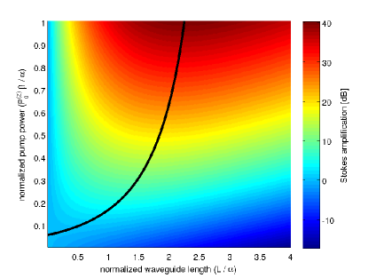
Figure 1: Stokes amplification in decibel of a waveguide that is subject to linear loss and 2PA as a function of the pump power level and the waveguide length in natural units for a SBS gain of $\Gamma=20\beta$. Note that for every fixed pump power above a certain threshold, the amplification grows with increasing waveguide length, reaches a maximum and then drops off again. These maxima indicate optimal waveguide lengths and are connected with a solid black line.

First, we investigate the case that the material does not exhibit fifth-order loss. This applies for example to glasses, including the chalcogenide rib waveguides that are the basis of recent on-chip SBS activities Eggleton2013 , or to semiconductors illuminated below the half-bandgap. This case implies $\{\alpha,\beta\}\neq 0$; $\gamma=0$. The resulting equation for the pump power is:

$$\partial_{z}{P}^{(2)}+\alpha{P}^{(2)}+\beta[{P}^{(2)}]^{2}=0.$$ (36)

This is an equation of the Riccati type and can therefore be solved using the ansatz ${P}^{(2)}(z)=y^{\prime}/(\beta y)$, resulting in the solution

$${P}^{(2)}(z)= \frac{\alpha\exp(-\alpha z)}{\beta[\zeta-\exp(-\alpha z)]},$$ (37)

$$\text{where}\quad\zeta= 1+\frac{\alpha}{\beta{P}^{(2)}_{0}}$$ (38)

parametrises the input pump power. Next, we insert this result in the Stokes equation:

$$\partial_{z}{P}^{(1)}= -\alpha\left[1-\frac{(\Gamma-2\beta)\exp(-\alpha z)}{\beta[\zeta-\exp(-\alpha z)]}\right]{P}^{(1)},$$ (39)

which can be readily solved:

$$\frac{\partial_{z}{P}^{(1)}}{{P}^{(1)}}= -\alpha\frac{\Gamma-2\beta}{\beta}\cdot\frac{\alpha\exp(-\alpha z)}{\zeta-\exp(-\alpha z)};$$ (40)

$${P}^{(1)}(z)= S^{{\text{2PA}}}\exp(-\alpha z)\left[\zeta-\exp(-\alpha z)\right]^{(\Gamma/\beta-2)},$$ (41)

where

$$S^{{\text{2PA}}}= {P}^{(1)}_{0}(\zeta-1)^{(2-\Gamma/\beta)}$$ (42)

parametrises the input Stokes power ${P}^{(1)}_{0}={P}^{(1)}(0)$. From Eq. (41), we can readily derive the Stokes amplification in the presence of 2PA and linear loss:

$$\mathcal{A}_{\text{dB}}^{{\text{2PA}}+{\text{lin}}}(L)= \frac{10}{\ln 10}\Bigg{\{}-\alpha L+\left(\Gamma-2\beta\right)\times$$ (43)

$$\quad\left[\ln\left(1+\beta{P}^{(2)}_{0}[1-\exp(-\alpha L)]/\alpha\right)\right]^{1/\beta}\Bigg{\}}.$$

This result comprises two parts: First the exponential decay of the Stokes power due to the linear loss $\alpha L$. Second, the effect of SBS and 2PA. The logarithm is always non-zero and can be interpreted so that 2PA and linear loss reduce the SBS-effective waveguide length and SBS-effective pump power; it grows monotonically as a function of the waveguide length $L$ and the pump power ${P}^{(2)}_{0}$, but saturates for $\alpha L\gg 1$ while being unbounded with respect to ${P}^{(2)}_{0}$. The prefactor $(\Gamma-2\beta)$ finally is the central result of this analysis. It states that the SBS-gain of a waveguide with 2PA present is effectively reduced by twice the 2PA-coefficient: $\Gamma_{\text{eff}}=\Gamma-2\beta$. Thus, SBS can only be observed if $\Gamma/(2\beta)>1$. Therefore, although any level of total Stokes amplification can be obtained by increasing the pump power, increasing the waveguide length much beyond $1/\alpha$ is not useful. To illustrate this, the general dependence of $\mathcal{A}_{\text{dB}}^{({\text{2PA}}+{\text{lin}})}$ for an arbitrary chosen ratio between SBS gain and 2PA-coefficient of $\Gamma=20\beta$ is depicted in Fig. 1 over a wide range of waveguide lengths and pump powers.

To conclude, we consider the case of vanishing linear loss $\alpha\rightarrow 0$. To this end, we approximate $\exp(-\alpha L)\approx 1-\alpha L$ in Eq. (41) and Eq. (43) to find:

$$\mathcal{A}_{\text{dB}}^{{\text{2PA}}}(L)= \frac{10}{\ln 10}\left(\frac{\Gamma}{\beta}-2\right)\ln\left(1+\beta L{P}^{(2)}_{0}\right)$$ (44)

with the corresponding Stokes amplitude

$${P}^{(1)}(z)= {P}^{(1)}_{0}\left[1+z\beta{P}^{(2)}_{0}\right]^{(\Gamma/\beta-2)}.$$ (45)

We state this result to point out that in the case of 2PA as the only loss mechanism, the solution is algebraic rather than transcendental and that any arbitrary exponent can be realised. For example, it is possible to connect the Stokes power linearly or quadratically to the pump power by choosing $\Gamma=3\beta$ or $\Gamma=4\beta$, respectively. We cannot think of any useful application for this analog computation, but find it an amusing curiosity.

III.2 SBS with FCA alone

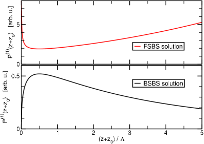
Figure 2: Solution to the problem of SBS with free carrier absorption in the forward SBS (top panel) and backward SBS (bottom panel) configuration for the solution normalisation constant set to $S^{\text{FCA}}=\sqrt{\Lambda}$. Note the respective extrema of the solutions at $z+z_{0}=\Lambda/2$.

Next, we focus on the case $\{\alpha,\beta\}=0$; $\gamma\neq 0$, which describes a system subject only to 2PA-induced free carrier absorption, but neither linear loss nor 2PA itself: 2PA is assumed to generate carriers but not absorb a noticeable amount of energy itself. The following discussion is intended as a preparation for the discussion of 2PA-induced FCA in combination with linear loss in Section III.3 and for the qualitative discussion in Section III.4. The results can also be directly applied to situations where both $\alpha$ and $\beta$ are very small, e.g. for very good semiconductor waveguides.

Within this section, the pump power satisfies the equation

$$\partial_{z}{P}^{(2)}=-\gamma[{P}^{(2)}]^{3},$$ (46)

which has the solution

$${P}^{(2)}(z)= \frac{1}{\sqrt{2\gamma(z+z_{0})}},$$ (47)

$$\text{where}\quad z_{0}= \frac{1}{2\gamma({P}^{(2)}_{0})^{2}}$$ (48)

again parametrises the input pump power. Note that negative values for $z_{0}$ are unphysical, because $\gamma$ is positive. It is convenient to express lengths and powers in terms of the respective natural units of $\Lambda$ (length) and $\Pi$ (power):

$$\Lambda= \gamma/\Gamma^{2}, \Pi= \Gamma/\gamma.$$ (49)

Next, we insert Eq. (47) into Eq. (34) to obtain:

$$\frac{\partial_{z}{P}^{(1)}}{{P}^{(1)}}=-\frac{1}{2(z+z_{0})}+\frac{\Gamma}{\sqrt{2\gamma(z+z_{0})}},$$ (50)

The solution to this equation is

$${P}^{(1)}(z)= \frac{S^{{\text{FCA}}}}{\sqrt{z+z_{0}}}\exp\left[\Gamma\sqrt{2(z+z_{0})/\gamma}\right],$$ (51)

with the normalisation constant

$$S^{{\text{FCA}}}= {P}^{(1)}_{0}\sqrt{z_{0}}\exp\left[-\Gamma\sqrt{2z_{0}/\gamma}\right].$$ (52)

This solution Eq. (51) is plotted in the top panel of Fig. 2 for $S^{\text{FCA}}=\sqrt{\Lambda}$ directly above the inverse of Eq. (51), i.e. the solution to the BSBS problem. The first feature of Eq. (51) is that the general shape of the solution is universal for SBS-waveguides with free carrier absorption. Within this plot the waveguide corresponds a window starting at $z_{0}/\Lambda$ (defined by the pump power) and of length $L/\Lambda$. Increasing the pump power simply moves the window to the left of the plot. Variations in the SBS-gain, the FCA-coefficient and the injected Stokes power only rescale the plot axes. The second crucial feature of the solution is the extremum at $z+z_{0}=\Lambda/2$. This means that in a strongly pumped waveguide the Stokes amplitude assumes its minimum somewhere inside the waveguide and grows towards both ends. Furthermore, for very high pump levels, the Stokes amplitude at the output is lower than at the input, which means that any SBS-gain inside the waveguide is destroyed by free carrier absorption if the pump is too strong for a given waveguide length.

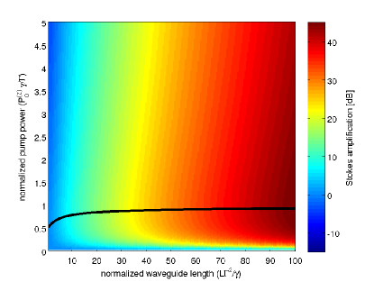
Figure 3: Stokes amplification in decibel of a waveguide whose only loss mechanism is 2PA-induced free carrier absorption (2PA itself neglected) as a function of the pump power level and the waveguide length in natural units. Please note that for every fixed waveguide length, the amplification grows with increasing pump power, reaches a maximum and then drops off again. These maxima correspond to optimal pump power levels and are connected with a solid black line.

The Stokes amplification of the waveguide can be derived from Eq. (51); we find

$$\mathcal{A}_{\text{dB}}^{{\text{FCA}}}(L)= \frac{10}{\ln 10}\bigg{\{}\frac{\Gamma}{\gamma{P}^{(2)}_{0}}\left[\sqrt{2\gamma L({P}^{(2)}_{0})^{2}+1}-1\right]$$

$$\quad-\frac{1}{2}\ln[1+2\gamma L({P}^{(2)}_{0})^{2}]\bigg{\}}.$$ (53)

This function is shown in Fig. 3 for a wide range of waveguide lengths $L$ and pump powers ${P}^{(2)}_{0}$. As in Fig. 2, this plot has been made universal for any combination of SBS and FCA coefficients. As a consequence of the non-monotonic nature of Eq. (51), the Stokes amplification $\mathcal{A}_{\text{dB}}^{{\text{FCA}}}$ assumes a maximum at a specific pump power for every given waveguide length. These optimal pump powers can be computed by solving the equation

$$\left[\frac{\partial\mathcal{A}_{\text{dB}}^{{\text{FCA}}}(L,{P}^{(2)}_{0})}{\partial{P}^{(2)}_{0}}\right]_{L}=0$$ (54)

with $L$ kept fixed. Since a closed analytical solution to this cannot be found, we use Newton’s method to find the zeros. However, it can be shown that the optimum pump powers always lies inside the interval $1/2\leq\gamma^{-1}\Gamma{P}^{(2)}_{0}\leq 1$. The numerically determined optimal pump powers are highlighted in Fig. 3 with a solid black line.

III.3 SBS with FCA and linear loss

After the discussion of FCA as the only loss mechanism, we now add linear loss, i.e. we study the situation $\beta=0$; $\{\alpha,\gamma\}\neq 0$. This is the most general case involving FCA that still can be solved analytically. In Section III.4, we present a perturbative treatment of weak 2PA alongside strong linear loss and FCA based on the expressions derived in this section.

As before, we start with solving the equation for the pump power along the waveguide:

$$\partial_{z}{P}^{(2)}=-\alpha{P}^{(2)}-\gamma[{P}^{(2)}]^{3}.$$ (55)

This can be transformed into a Riccati equation via a substitution of the type $u=[{P}^{(2)}]^{2}$. The closed solution is:

$${P}^{(2)}(z)= \frac{{P}^{(2)}_{0}\sqrt{\alpha}}{\sqrt{\big{(}\gamma[{P}^{(2)}_{0}]^{2}+\alpha\big{)}\exp\big{(}2\alpha z\big{)}-\gamma[{P}^{(2)}_{0}]^{2}}}.$$ (56)

Next, we solve for the Stokes power along the waveguide by integrating the equation

$$\frac{\partial_{z}{P}^{(1)}}{{P}^{(1)}}=-\alpha+\Gamma{P}^{(2)}-\gamma[{P}^{(2)}]^{2},$$ (57)

to obtain

$${P}^{(1)}(z)= S^{{\text{FCA}}+{\text{lin}}}{P}^{(2)}(z)\times$$

$$\quad\exp\left\{\frac{\Gamma}{\sqrt{\alpha\gamma}}\tan^{-1}\left[\frac{\sqrt{\alpha}}{\sqrt{\gamma}{P}^{(2)}(z)}\right]\right\},$$ (58)

where the input Stokes power enters via the normalisation constant

$$S^{{\text{FCA}}+{\text{lin}}}= \frac{{P}^{(1)}_{0}}{{P}^{(2)}_{0}}\exp\left\{-\frac{\Gamma}{\sqrt{\alpha\gamma}}\tan^{-1}\left[\frac{\sqrt{\alpha}}{\sqrt{\gamma}{P}^{(2)}_{0}}\right]\right\}.$$ (59)

The spatial evolution of the Stokes wave is qualitatively similar to the one depicted in Fig. 2. By taking the decadic logarithm of Eq. (58) including Eq. (59), one can directly obtain the explicit relationship between the total Stokes amplification $\mathcal{A}_{\text{dB}}^{{\text{FCA}}+{\text{lin}}}$ and the waveguide length and the pump power. This expression is long and convoluted and does not provide any additional insight, so we forgo showing it here. As before, it is very useful to introduce the problem-specific units of length and power stated in Eq. (49) as the natural unit system. Consequently, the linear loss is best expressed in natural units of inverse length:

$$\Upsilon=\alpha\gamma\Gamma^{-2}.$$ (60)

If this normalised linear loss vanishes, the plot of $\mathcal{A}_{\text{dB}}^{{\text{FCA}}+{\text{lin}}}$ is identical to the previous result Fig. 3. As the linear loss increases, the total amplification decays not only for increasing pump power but also for increasing waveguide length, leading to a well defined maximal obtainable amplification for each value $\Upsilon$. The maximal amplification is obtained for exactly one pair of optimal pump power $P^{({\text{opt}})}$ and optimal waveguide length $L^{({\text{opt}})}$. This is illustrated in Fig. 4 for the case of $\Upsilon=0.03$. We will resume this topic in Section IV.2.

III.4 SBS with FCA, linear loss and weak 2PA

Finally, we turn towards the case that all three loss mechanisms (linear loss, 2PA and FCA) are present. In this case, the equation for ${P}^{(2)}(z)$ can only be derived implicitly, i.e. in the form $z({P}^{(2)})$, but not explicitly. Unfortunately, this makes it impossible to solve the general case exactly. One therefore has to resort to approximate solutions derived from numerical calculations or perturbation theory in the parameter $\beta$. To zeroth order in $\beta$, the pump profile ${P}^{(2)}(z)$ can be adopted from the 2PA-free case Eq. (47). This is because we assume that the impact of 2PA on the pump is of the same order as the (neglected) pump-depletion due to SBS. Under this assumption, the SBS-gain $\Gamma$ is simply reduced by twice the 2PA-coefficient:

$$\Gamma_{\text{eff}}=\Gamma-2\beta.$$ (61)

All solutions from Section III.3 apply directly with this substitution.

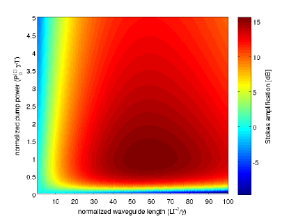
Figure 4: Stokes amplification in decibel of a waveguide that is subject to linear loss and 2PA-induced free carrier absorption (2PA itself neglected) as a function of the pump power level and the waveguide length in natural units for a normalised linear loss $\Upsilon=\alpha\gamma\Gamma^{-2}=0.03$. To illustrate the impact of linear loss, we adopted the colorbar from Fig. 3. There is one optimal combination of waveguide length $L^{({\text{opt}})}\approx 60\gamma\Gamma^{-2}$ and pump power $P^{({\text{opt}})}\approx\Gamma/\gamma$ that leads to the maximally realisable Stokes amplification of about $15\text{ dB}$ for this value of $\Upsilon$, which corresponds to a figure of merit (see Section IV.2 for details) of $\mathcal{F}_{\text{FCA}}\approx 2.9$.

The next perturbation order would involve a first order correction to the pump profile ${P}^{(2)}(z)$. While this can be found, the subsequent equation for the Stokes amplitude ${P}^{(1)}(z)$ and as a consequence the equation for the total Stokes amplification involve an integral that does not have a closed solution. For this reason, we adhere to the zeroth order approximation and refer the reader to numerical solutions whenever more accurate results are required.

IV Design guidelines and figures of merit

In this section, we provide guidelines for the optimal choice of waveguide length and pump power of waveguides whose SBS gain and loss coefficients have either been measured or computed numerically using the expressions in Ref. Wolff2015a and the Appendices of this paper. We furthermore provide figures of merit that express the suitability of any given material or waveguide design for the purpose of SBS in a single number.

IV.1 SBS with 2PA and linear loss

In the absence of fifth-order loss (especially 2PA-induced FCA), we can apply the results from Section III.1. This covers most centrosymmetric and amorphous insulators including glasses. The main feature of Eq. (43) is that it is monotonic and unbounded with respect to the pump power. Thus, the SBS gain of any given waveguide can in principle be increased indefinitely by injecting a sufficiently strong pump, provided the SBS gain is sufficient to overcome the loss due to 2PA. In other words, any material or waveguide design is capable of exhibiting SBS if the figure of merit

$$\mathcal{F}_{\text{2PA}}=\frac{\Gamma}{2\beta}$$ (62)

is greater than one. In every material or waveguide design with $\mathcal{F}_{\text{2PA}}<1$, SBS is quenched by 2PA. For $\mathcal{F}_{\text{2PA}}=1$, SBS and 2PA cancel each other to leading order; higher order corrections predict a weak power-dependent decay of the Stokes wave in this regime.

The total Stokes amplification does not grow indefinitely with respect to waveguide length, because the linear term $-\alpha L$ in Eq. (43) at some point overcomes the saturating logarithm of the second term. The optimal waveguide length $L^{({\text{opt}})}$ is given by the condition

$$\frac{\partial\mathcal{A}_{\text{dB}}^{{\text{2PA}}+{\text{lin}}}}{\partial L}=0,$$ (63)

which can be evaluated exactly:

$$L^{({\text{opt}})}= \frac{1}{\alpha}\ln\left[\frac{{P}^{(2)}_{0}(\Gamma-\beta)}{(\beta{P}^{(2)}_{0}+\alpha)}\right]$$ (64)

$$\ \xrightarrow{{P}^{(2)}_{0}\gg\alpha/\beta}\ \frac{\ln(2\mathcal{F}_{\text{2PA}}-1)}{\alpha}.$$ (65)

This means that the optimal waveguide length depends logarithmically on the pump power, but will always remain in the vicinity of $\alpha^{-1}$. The power-dependence of the optimal waveguide length for the case of $\mathcal{F}_{\text{2PA}}=10$ is shown in Fig. 1 as a black solid line.

IV.2 SBS with FCA, linear loss and weak 2PA

In most indirect semiconductors such as silicon and germanium, the long carrier lifetime leads to the effect that the free carriers created by 2PA have a much stronger impact on the absorption of a quasi-CW light wave than the two-photon absorption itself. Although this effect can be reduced by extracting free carriers via an externally applied electric field, the loss due to 2PA-induced FCA will still surpass the 2PA itself in many situations and the results from Section III.4 can be applied.

In contrast to the previous section, the total Stokes amplification of a waveguide that experiences FCA is non-monotonic with power and is in fact bounded with respect to both the injected pump power and its length. For each set of SBS gain and loss parameters, there is exactly one choice of length and pump power that leads to the maximal gain, as can be seen in Fig. 4.

In any given material or waveguide design, a total Stokes amplification can be obtained only if the FCA figure of merit

$$\mathcal{F}_{\text{FCA}}=\frac{\Gamma-2\beta}{2\sqrt{\alpha\gamma}}$$ (66)

is greater than 1. As shown in Wolff2015b , this quantity emerges naturally as a figure of merit from Eqs. (II.2). Unlike the situation without FCA (see Section IV.1), $\mathcal{F}_{\text{FCA}}$ merit also implies an absolute maximum for the Stokes amplification that can be obtained with a given waveguide design. It is attained for the optimal choice of waveguide length and pump power, both of which depend on $\mathcal{F}_{\text{FCA}}$. This interdependence is discussed in a separate paper Wolff2015b .

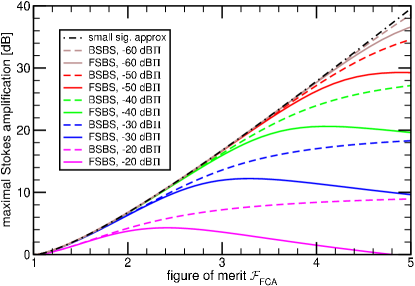
Figure 5: Stokes amplification plots for linear loss, FCA and weak 2PA: Comparison of the maximally realisable amplification within the small-signal approximation (black dash-dotted line) and corresponding maximal amplifications in FSBS (solid lines) and BSBS (dashed lines) configuration for finite Stokes input powers between $-60\,\text{dB}$ and $-20\,\text{dB}$ of the natural power unit $\Pi=\Gamma_{\text{eff}}/\gamma=(\Gamma-2\beta)/\gamma$.

In Fig. 5, we compare the maximally realisable Stokes amplification predicted by our small-signal approximation with results obtained by numerically solving the large-signal equations Eqs. (12, 13) for the analytically predicted operating conditions and injected Stokes powers between $-60\,\text{dB}$ and $-20\,\text{dB}$ of the natural power unit $\Pi$ both in forward and backward configuration. In the case of FSBS, we employed a simple 4-th order Runge-Kutta integrator. In the case of BSBS, we used the shooting method based on a variable order Runge-Kutta that is optimised for stiff differential equations. It is clearly visible how the small-signal solution provides an upper bound for the realisable Stokes amplification. The difference can be attributed to energy transfer from the pump to the Stokes (known as pump depletion in SBS without loss) and additional carrier generation due to the relatively high Stokes intensity. Finally, we note that the optimal operating conditions (i.e. waveguide length and pump power) shift as the input Stokes level is increased and that this affects forward SBS and backward SBS quite differently. This is because the small-signal approximation no longer applies over the full range of $\mathcal{F}_{\text{FCA}}$ and input Stokes powers. In the case of BSBS, the amplification maximum as a function of waveguide length and pump power remains very flat, which means that the analytical prediction is very viable. However, in the case of FSBS the amplification maximum becomes fairly sharp and the waveguide has to be shortened to obtain performance that is comparable to the BSBS amplification shown in Fig. 5. In other words: A forward SBS amplifier has a smaller dynamic range than an amplifier based on backward SBS.

V Conclusions

In this paper, we have discussed the impact of nonlinear optical loss on the process of SBS within a small-signal approximation. Based on analytical solutions to this problem, we have derived figures of merit that describe the suitability of a material or a waveguide design for the case that fifth-order nonlinear loss effects such as 2PA-induced FCA can be neglected and the case that they cannot. In the former case, we find that, although third-order loss reduces the total Stokes wave amplification along the waveguide, the amplification is not fundamentally restricted and can be increased indefinitely by increasing pump power until the weakest component in the optical circuit is permanently damaged. In the latter case, however, the Stokes amplification due to SBS is overcome by FCA once some optimal pump power is exceeded. Thus, the total amplification is bounded to a value that is ultimately given by the figure of merit $\mathcal{F}_{\text{FCA}}=(\Gamma-2\beta)/\sqrt{4\alpha\gamma}$. This opens basically three possible routes to effective SBS-circuits in semiconductor (especially silicon) photonics platforms. First, the upper amplification bound can be increased by reducing the linear loss $\alpha$. This often is a challenging task. Second, the impact of FCA could be drastically reduced by removing the free carriers by means of an externally applied electric field. The resulting increase in linear loss would be tolerable as long as the product $\alpha\gamma$ is reduced. The third, and on a short time scale potentially most viable, solution would be to design future silicon photonic circuits for SBS to operate at wavelengths below the 2PA-threshold, e.g. around $2400\,\text{nm}$ for the case of silicon. This would eliminate not only 2PA (which itself is not problematic), but in particular the induced FCA and lead to higher acoustic quality factors due to the reduced acoustic frequency.

Appendix A Expressions for loss coefficients

In the following Appendices, we derive the loss coefficients that appear in Eq. (3) and Eq. (4). The explicit expressions are:

$$\tilde{\alpha}_{i}= \frac{\varepsilon_{0}\omega}{{{\mathcal{P}}}^{(i)}}\int{\rm{d}}^{2}r\ \big{|}{\widetilde{{\bf{e}}}}^{(i)}\big{|}^{2}\Im\{\varepsilon_{r}\},$$ (67)

$$\tilde{\beta}_{ij}= \frac{1}{{{\mathcal{P}}}^{(i)}}\int{\rm{d}}^{2}r\ \big{(}\big{|}{\widetilde{{\bf{e}}}}^{(i)}\cdot{\widetilde{{\bf{e}}}}^{(j)}\big{|}^{2}+\big{|}{\widetilde{{\bf{e}}}}^{(i)}\cdot({\widetilde{{\bf{e}}}}^{(j)})^{\ast}\big{|}^{2}+\big{|}{\widetilde{{\bf{e}}}}^{(i)}\big{|}^{2}\big{|}{\widetilde{{\bf{e}}}}^{(j)}\big{|}^{2}\big{)}\Sigma^{\text{2PA}},$$ (68)

$$\tilde{\gamma}_{ijk}= \frac{1}{{{\mathcal{P}}}^{(i)}}\int{\rm{d}}^{2}r\ |{\widetilde{{\bf{e}}}}^{(i)}|^{2}\Big{[}|{\widetilde{{\bf{e}}}}^{(j)}\cdot{\widetilde{{\bf{e}}}}^{(k)}|^{2}+|{\widetilde{{\bf{e}}}}^{(j)}\cdot({\widetilde{{\bf{e}}}}^{(k)})^{\ast}|^{2}+|{\widetilde{{\bf{e}}}}^{(j)}|^{2}|{\widetilde{{\bf{e}}}}^{(k)}|^{2}\Big{]}\Sigma^{\text{FCA}},$$ (69)

where the indices $i$, $j$ and $k$ label the respective optical eigenmodes modes and can take the values 1 and 2. The Symbols $\Sigma^{\text{2PA}}$ and $\Sigma^{\text{FCA}}$ are nonlinear conductivities associated with 2PA and 2PA-induced FCA and are expressed in more conventional terms in Eq. (71) and Eq. (78), respectively. The values

$$\Sigma^{\text{2PA}}= 5.5\cdot 10^{-16}\,\text{W}\text{m}^{3}\text{V}^{-4}, \Sigma^{\text{FCA}}= 6.0\cdot 10^{-28}\,\text{W}\text{m}^{5}\text{V}^{-6},$$ (70)

correspond to a bulk 2PA-coefficient of $5\cdot 10^{-12}\text{ m/W}$ and an electron scattering cross section of $1.45\cdot 10^{-21}\text{ m}^{2}$ together with a carrier life time of $10\,\text{ns}$. Those are typical literature values Jalali2005 for silicon at a vacuum wavelength of $1550\text{ nm}$.

Appendix B Derivation of 2PA-terms

In time-domain it is sometimes advantageous to represent lossy (i.e. dispersive) optical nonlinearities is via a nonlinear current distribution Taflove2005 . The corresponding nonlinear conductivity to represent 2PA is related to the imaginary part of the third-order susceptibility:

$$\Sigma^{{\text{2PA}}}=\omega\varepsilon_{0}\Im\{\chi^{(3)}\}.$$ (71)

Here, we neglected the tensorial nature of $\chi^{(3)}$ in order to to improve the readability of the integrals (67–69). The generalisation to tensorial nonlinearities is a matter of book-keeping. With this, we find the real-valued time-domain current density ${\bf{J}}^{\text{2PA}}(t)=-\Sigma^{\text{2PA}}|{\bf{E}}(t)|^{2}{\bf{E}}(t),$ where for the sake of brevity, we wrote ${\bf{v}}^{2}={\bf{v}}\cdot{\bf{v}}$ and $|{\bf{v}}|^{2}={\bf{v}}^{\ast}\cdot{\bf{v}}$ for any vectorial quantity ${\bf{v}}$. The electric field is formed by the interference between two optical eigenmodes: ${\bf{E}}(t)={a}^{(1)}{{\bf{e}}}^{(1)}+{a}^{(2)}{{\bf{e}}}^{(2)}+{\rm{c.c.}}.$ Within a coupled-mode theory, we need the projection of ${\bf{J}}^{\text{2PA}}$ on the optical eigenmodes, e.g. ${{\bf{e}}}^{(1)}$:

$$\langle{e}^{(1)}|{\bf{J}}^{\text{2PA}}\rangle= -\Big{\langle}\ {\int{\rm{d}}^{3}r\ \left[({{\bf{e}}}^{(1)})^{\ast}\cdot({a}^{(1)}{{\bf{e}}}^{(1)}+{a}^{(2)}{{\bf{e}}}^{(2)}+{\rm{c.c.}})\right]\Sigma^{\text{2PA}}\big{|}{a}^{(1)}{{\bf{e}}}^{(1)}+{a}^{(2)}{{\bf{e}}}^{(2)}+{\rm{c.c.}}\big{|}^{2}}\ \Big{\rangle}_{T_{\text{ac}}}$$ (72)

$$= -\Big{\langle}2{a}^{(1)}\int{\rm{d}}^{3}r\ \big{|}{{\bf{e}}}^{(1)}\big{|}^{2}\Sigma^{\text{2PA}}\left[\big{|}{a}^{(1)}\big{|}^{2}\big{|}{{\bf{e}}}^{(1)}\big{|}^{2}+\big{|}{a}^{(2)}\big{|}^{2}\big{|}{{\bf{e}}}^{(2)}\big{|}^{2}\right]$$

$$\quad+\big{(}{a}^{(1)}\big{)}^{\ast}\int{\rm{d}}^{3}r\ \big{(}{{\bf{e}}}^{(1)}\cdot{{\bf{e}}}^{(1)}\big{)}^{\ast}\Sigma^{\text{2PA}}\big{(}{a}^{(1)}\big{)}^{2}{{\bf{e}}}^{(1)}\cdot{{\bf{e}}}^{(1)}$$

$$\quad+2{a}^{(2)}\int{\rm{d}}^{3}r\ \big{(}{{\bf{e}}}^{(1)}\big{)}^{\ast}\cdot{{\bf{e}}}^{(2)}\Sigma^{\text{2PA}}{a}^{(1)}\big{(}{a}^{(2)}\big{)}^{\ast}{{\bf{e}}}^{(1)}\cdot\big{(}{{\bf{e}}}^{(2)}\big{)}^{\ast}$$

$$\quad+2\big{(}{a}^{(2)}\big{)}^{\ast}\int{\rm{d}}^{3}r\ \big{(}{{\bf{e}}}^{(1)}\cdot{{\bf{e}}}^{(2)}\big{)}^{\ast}\Sigma^{\text{2PA}}{a}^{(1)}{a}^{(2)}{{\bf{e}}}^{(1)}\cdot{{\bf{e}}}^{(2)}$$

$$\quad+\text{oscillating terms}\Big{\rangle}_{T_{\text{ac}}}$$ (73)

$$= {a}^{(1)}\big{|}{a}^{(1)}\big{|}^{2}\ \int{\rm{d}}^{2}r\ \Sigma^{\text{2PA}}\big{(}2\big{|}{\widetilde{{\bf{e}}}}^{(1)}\cdot({\widetilde{{\bf{e}}}}^{(1)})^{\ast}\big{|}^{2}+\big{|}{\widetilde{{\bf{e}}}}^{(1)}\cdot{\widetilde{{\bf{e}}}}^{(1)}\big{|}^{2}\big{)}$$

$$\quad+2{a}^{(1)}\big{|}{a}^{(2)}\big{|}^{2}\ \int{\rm{d}}^{2}r\ \Sigma^{\text{2PA}}\big{(}\big{|}{\widetilde{{\bf{e}}}}^{(1)}\cdot{\widetilde{{\bf{e}}}}^{(2)}\big{|}^{2}+\big{|}{\widetilde{{\bf{e}}}}^{(1)}\cdot({\widetilde{{\bf{e}}}}^{(2)})^{\ast}\big{|}^{2}+\big{|}{\widetilde{{\bf{e}}}}^{(1)}\big{|}^{2}\big{|}{\widetilde{{\bf{e}}}}^{(2)}\big{|}^{2}\big{)}.$$ (74)

The projection on the other mode ${{\bf{e}}}^{(2)}$ follows from this by interchanging the mode index superscripts.

Appendix C Derivation of FCA-terms

As in Appendix B we intend to describe the loss via a time domain current density ${\bf{J}}^{\text{FCA}}$. It is due to the conductivity of a dilute plasma with carrier density $N_{\text{c}}$, which can be described Tinten2000 using a Drude-Sommerfeld model with effective carrier mass $m^{\ast}$ and damping parameter $\omega_{\text{d}}$:

$${\bf{J}}^{\text{FCA}}(t)=-\frac{\omega_{\text{d}}q^{2}N_{\text{c}}}{(\omega^{2}+\omega^{2}_{\text{d}})m^{\ast}}{\bf{E}}(t).$$ (75)

Here, $q$ is the elementary charge and the parameters $m^{\ast}$, $\omega_{\text{d}}$ are material specific and therefore may depend on position within the waveguide. The carriers are created by two-photon absorption and destroyed via recombination on a time scale $\tau_{\text{c}}>10\text{ns}$. The order of this time constant is important because it covers around $100$ acoustic cycles for typical Stokes shifts of $3-30\text{GHz}$. Consequently, the carrier density is to be derived from the 2PA power loss averaged over a time-scale greater than one acoustic period:

$$P^{\text{2PA}}_{\text{loss}}= -\Big{\langle}\ {{\bf{E}}(t)\cdot{\bf{J}}^{\text{2PA}}(t)}\ \Big{\rangle}_{T_{\text{ac}}}=\Sigma^{\text{2PA}}\Big{\langle}\ {|{\bf{E}}(t)|^{2}|{\bf{E}}(t)|^{2}}\ \Big{\rangle}_{T_{\text{ac}}}$$ (76)

$$= 2\Sigma^{\text{2PA}}\bigg{\{}|{a}^{(1)}|^{4}\Big{[}|{{\bf{e}}}^{(1)}\cdot{{\bf{e}}}^{(1)}|^{2}+2(|{{\bf{e}}}^{(1)}|^{2})^{2}\Big{]}\ +\ |{a}^{(2)}|^{4}\Big{[}|{{\bf{e}}}^{(2)}\cdot{{\bf{e}}}^{(2)}|^{2}+2(|{{\bf{e}}}^{(2)}|^{2})^{2}\Big{]}$$

$$\quad+4|{a}^{(1)}|^{2}|{a}^{(2)}|^{2}\Big{[}|{{\bf{e}}}^{(1)}\cdot{{\bf{e}}}^{(2)}|^{2}+|{{\bf{e}}}^{(1)}|^{2}|{{\bf{e}}}^{(2)}|^{2}+|{{\bf{e}}}^{(1)}\cdot({{\bf{e}}}^{(2)})^{\ast}|^{2}\Big{]}\bigg{\}}.$$ (77)

The carrier generation rate is this optical power loss divided by twice the photon energy, whereas the carrier recombination rate is determined by $N_{c}$ itself and the carrier life time $\tau_{c}$: $\partial_{t}N_{c}=P^{\text{2PA}}_{\text{loss}}/(2\hbar\omega)-\frac{N_{c}}{\tau_{c}}.$ Note that the carrier life typically is reduced near material interfaces and therefore position dependent. In our crude model we neglected carrier diffusion. If the field amplitudes vary on time scales larger than $\tau_{c}$, the loss due to FCA is given by the equilibrium carrier density $N_{c}^{\text{(eq)}}=\tau_{c}P^{\text{2PA}}_{\text{loss}}/(2\hbar\omega).$ This allows us to express the FCA-related nonlinear conductivity:

$$\Sigma^{\text{FCA}}=\frac{\omega_{\text{d}}\tau_{\text{c}}q^{2}\Sigma^{\text{2PA}}}{2\hbar\omega(\omega^{2}+\omega^{2}_{\text{d}})m^{\ast}}.$$ (78)

Within the context of our coupled mode theory, we require the projection of the FCA-current on the optical eigenmodes, e.g. the mode ${{\bf{e}}}^{(1)}$:

$$\langle{e}^{(1)}|{\bf{J}}^{\text{FCA}}\rangle= -\frac{1}{2\hbar\omega}\Big{\langle}\ {\int{\rm{d}}^{3}r\ [{{\bf{e}}}^{(1)}]^{\ast}\cdot[{a}^{(1)}{{\bf{e}}}^{(1)}+{a}^{(2)}{{\bf{e}}}^{(2)}+{\rm{c.c.}}]\frac{\omega_{\text{d}}q^{2}\tau_{\text{c}}}{2\hbar\omega(\omega^{2}+\omega_{\text{d}}^{2})m^{\ast}}P^{\text{2PA}}_{\text{loss}}}\ \Big{\rangle}_{T_{\text{opt}}}$$ (79)

$$= -\frac{{a}^{(1)}|{a}^{(1)}|^{4}}{\hbar\omega}\int{\rm{d}}^{2}r\ |{\widetilde{{\bf{e}}}}^{(1)}|^{2}\Sigma^{\text{FCA}}\Big{[}|{\widetilde{{\bf{e}}}}^{(1)}\cdot{\widetilde{{\bf{e}}}}^{(1)}|^{2}+2(|{\widetilde{{\bf{e}}}}^{(1)}|^{2})^{2}\Big{]}$$

$$\quad-\frac{{a}^{(1)}|{a}^{(2)}|^{4}}{\hbar\omega}\int{\rm{d}}^{2}r\ |{\widetilde{{\bf{e}}}}^{(1)}|^{2}\Sigma^{\text{FCA}}\Big{[}|{\widetilde{{\bf{e}}}}^{(2)}\cdot{\widetilde{{\bf{e}}}}^{(2)}|^{2}+2(|{\widetilde{{\bf{e}}}}^{(2)}|^{2})^{2}\Big{]}$$

$$\quad-\frac{4{a}^{(1)}|{a}^{(1)}|^{2}|{a}^{(2)}|^{2}}{\hbar\omega}\int{\rm{d}}^{2}r\ |{\widetilde{{\bf{e}}}}^{(1)}|^{2}\Sigma^{\text{FCA}}\Big{[}|{\widetilde{{\bf{e}}}}^{(1)}\cdot{\widetilde{{\bf{e}}}}^{(2)}|^{2}+|{\widetilde{{\bf{e}}}}^{(1)}|^{2}|{\widetilde{{\bf{e}}}}^{(2)}|^{2}+|{\widetilde{{\bf{e}}}}^{(1)}\cdot({\widetilde{{\bf{e}}}}^{(2)})^{\ast}|^{2}\Big{]}.$$ (80)

References

- (1) T. J. Kippenberg and K. J. Vahala, “Cavity Optomechanics: Back-Action at the Mesoscale, ” 321, 1172–1176 (2008).
- (2) B. J. Eggleton, C. G. Poulton, and R. Pant, “Inducing and harnessing stimulated Brillouin scattering in photonic integrated circuits,” Advances in Optics and Photonics 5, 536–587 (2013).
- (3) R. W. Boyd, Nonlinear optics (Academic, 3rd ed., 2003).
- (4) L. Brillouin. “Diffusion de la lumière par un corps transparent homogène,” Annals of Physics 17, 88–122 (1922).
- (5) R. Y. Chiao, C. H. Townes, and B. P Stoicheff, “Stimulated Brillouin scattering and coherent generation of intense hypersonic waves,” Phys. Rev. Lett. 12, 592 (1964).
- (6) G. P. Agrawal, Nonlinear fiber optics (Academic, 5th ed., 2012).
- (7) R. Pant, C. G. Poulton, D.-Y. Choi, H. Mcfarlane, S. Hile, E. Li, L. Thévenaz, B. Luther-Davies, S. J. Madden, and B. J. Eggleton, “On-chip stimulated Brillouin scattering,” Opt. Express 19, 8285–8290 (2011).
- (8) P. T. Rakich, C. Reinke, R. Camacho, P. Davids, and Z. Wang, “Giant enhancement of stimulated Brillouin scattering in the subwavelength Limit,” Phys. Rev. X 2, 011008 (2012).
- (9) H. Shin, W. Qiu, R. Jarecki, J. A. Cox, R. H. O. Ill, A. Starbuck, Z. Wang, and P. T. Rakich, “Tailorable stimulated Brillouin scattering in nanoscale silicon waveguides,” Nat. Commun. 4, 1944 (2013).
- (10) I. D. Rukhlenko, M. Premaratne, G. P. Agrawal, “Nonlinear Silicon Photonics: Analytical Tools,” IEEE J. Sel. Top. Quantum Electron. 16, 200–215 (2010).
- (11) R. Van Laer, B. Kuyken, D. Van Thourhout, and R. Baets, “Interaction between light and highly confined hypersound in a silicon photonic nanowire,” doi:10.1038/nphoton.2015.11, (2015).
- (12) I. V. Kabakova, R. Pant. D.-Y. Choi, S. Debbarma, B. Luther-Davies, S. J. Madden, and B. J. Eggleton, “Narrow linewidth Brillouin laser based on chalcogenide photonic chip,” Opt. Lett. 38, 3208–3211 (2013).
- (13) K. Hu, I. V. Kabakova, T. F. S. Büttner, S. Lefrancois, D. D. Hudson, S. He, and B. J. Eggleton, “Low-threshold Brillouin laser at 2m based on suspended-core chalcogenide fiber,” Opt. Lett. 39, 4651–4654 (2014).
- (14) T. F. S. Buettner, I. V. Kabakova, D. D. Hudson, R. Pant, C. G. Poulton, A. Judge, and B. J. Eggleton, “Phase-locking in Multi-Frequency Brillouin Oscillator via Four Wave Mixing,” Sci. Rep. 4, 5032 (2014).
- (15) X. Huang and S. Fan, “Complete all-optical silica fiber isolator via Stimulated Brillouin Scattering,” J. Lightwave Technol. 29, 2267–2275 (2011).
- (16) I. Aryanfar, C. Wolff, M. J. Steel, B. J. Eggleton, and C. G. Poulton, “Mode conversion using stimulated Brillouin scattering in nanophotonic silicon waveguides, ” Opt. Express 22, 29270–29282 (2014).
- (17) L. Thévenaz, “Slow and fast light in optical fibres,” Nature Photon. 2, 474–481 (2008).
- (18) B. Vidal, M. A. Piqueras, and J. Marti, “Tunable and reconfigurable photonic microwave filter based on stimulated Brillouin scattering,” Opt. Lett. 32, 23–25 (2007).
- (19) J. Li, H. Lee, and K. J. Vahala, “Microwave synthesizer using an on-chip Brillouin oscillator,” Nat. Commun. 4, 2097 (2013).
- (20) B. Morrison, D. Marpaung, R. Pant, E. Li, D.-Y. Choi, S. Madden, B. Luther-Davies, and B. J. Eggleton, “Tunable microwave photonic notch filter using on-chip stimulated Brillouin scattering,” Opt. Commun. 313, 85–89 (2014).
- (21) C. Wolff, M. J. Steel, B. J. Eggleton, and C. G. Poulton, “Stimulated Brillouin Scattering in integrated photonic waveguides: forces, scattering mechanisms and coupled mode analysis,” arXiv:1407.3521 [physics.optics], (2014).
- (22) C. Wolff, R. Soref, C. G. Poulton, and B. J. Eggleton, “Germanium as a material for stimulated Brillouin scattering in the mid-infrared, ” Opt. Express 22, 30735–30747 (2014).
- (23) C. Wolff, P. Gutsche, M. J. Steel, B. J. Eggleton, and C. G. Poulton, “Power limits and a figure of merit for stimulated Brillouin scattering in the presence of free carrier absorption, ” (in preparation)
- (24) D. Dimitropoulos, R. Jhaveri, R. Claps, J. C. S. Woo, and B. Jalali, “Lifetime of photogenerated carriers in silicon-on-insulator rib waveguides,” Appl. Phys. Lett. 86, 071115 (2005).
- (25) A. Taflove and S. C. Hagness Computational Electrodynamics (Artech House, 3rd ed., 2005)
- (26) K. Sokolowski-Tinten, D. von der Linde, “Generation of dense electron-hole plasmas in silicon, ” Phys. Rev. B 61, 2643 (2000).