Inflation in a modified radiative seesaw model

Abstract

A radiative seesaw model with an inert doublet dark matter is a promising candidate which could explain the existence of neutrino masses, dark matter and baryon number asymmetry of the Universe, simultaneously. In addition to these issues, inflation should also be explained since the recent CMB observations suggest the existence of the inflationary era at the early stage of the Universe. Thus, we extend it by a complex scalar field with a specific potential. This scaler could also be related to the neutrino mass generation at a TeV scale. We show that the inflation favored by the CMB observations could be realized even if inflaton takes sub-Plankian values during inflation.

I Introduction

Recent discovery of a Higgs-like particle higgs suggests that the framework of the standard model (SM) can describe Nature well up to the weak scale. On the other hand, we have experimental results which cannot be explained within it, that is, the existence of small neutrino masses t13 , the existence of dark matter (DM) uobs , and baryon number asymmetry in the Universe baryon . They require some extension of the SM. In our previous work, we show that a radiative seesaw model with an inert doublet Ma:2006km could be a promising candidate which can explain these problems, simultaneously Kashiwase:2012xd . The recent CMB observations suggest that the exponential expansion of the Universe occurs in the very early Universe. These results can constrain severely the allowed inflation models now Ade:2015lrj . Some inflationary models require the trans-Planckian field value for inflaton to realize the sufficient e-foldings. In this case, the Planck-suppressed operators become dominant and spoil the flatness of the inflaton potential. Thus, we consider its modification to realize the results from Planck by introducing inflaton with the sub-Planckian field value. We also show that the inflaton could play a crucial role for the neutrino mass generation other than the inflation.

II An extended model

The extended radiative seesaw model with a $Z_{2}$ odd complex scalar singlet $S$ is defined by the following $Z_{2}$ invariant terms Budhi:2014gxa :

$$-{\cal L}_{O} =-h_{\alpha i}\bar{N}_{i}H_{2}^{\dagger}L_{\alpha}-h_{\alpha i}^{*}\bar{L}_{\alpha}H_{2}N_{i}+\frac{1}{2}m_{N_{i}}\bar{N}_{i}N_{i}^{c}+\frac{1}{2}m_{N_{i}}^{*}\bar{N}_{i}^{c}N_{i},$$

$$+m_{1}^{2}|H_{1}|^{2}+m_{2}^{2}|H_{2}|^{2}+\lambda_{1}|H_{1}|^{4}+\lambda_{2}|H_{2}|^{4}+\lambda_{3}|H_{1}|^{2}|H_{2}|^{2}+\lambda_{4}|H_{1}^{\dagger}H_{2}|^{2}+\frac{\lambda_{5}}{2}\left[(H_{1}^{\dagger}H_{2})^{2}+h.c.\right],$$

$$-{\cal L}_{S} =\tilde{m}_{S}^{2}S^{\dagger}S+\frac{1}{2}m_{S}^{2}S^{2}+\frac{1}{2}m_{S}^{2}{S^{\dagger}}^{2}-\mu SH_{2}^{\dagger}H_{1}-\mu^{*}S^{\dagger}H_{1}^{\dagger}H_{2}$$

$$+\kappa_{1}(S^{\dagger}S)^{2}+\kappa_{2}(S^{\dagger}S)(H_{1}^{\dagger}H_{1})+\kappa_{3}(S^{\dagger}S)(H_{2}^{\dagger}H_{2}),$$ (1)

where $L_{\alpha}$ is a left-handed lepton doublet and $H_{2}$ is an inert doublet scalar. Since $H_{2}$ and right-handed neutrinos $N_{i}$ are assigned odd parity of $Z_{2}$ symmetry and all the SM contents including the ordinary Higgs doublet scalar $H_{1}$ are assigned even parity, neutrino Dirac mass terms are forbidden at tree level. Neutrino masses are generated through a one-loop diagram as shown in Fig. 1.

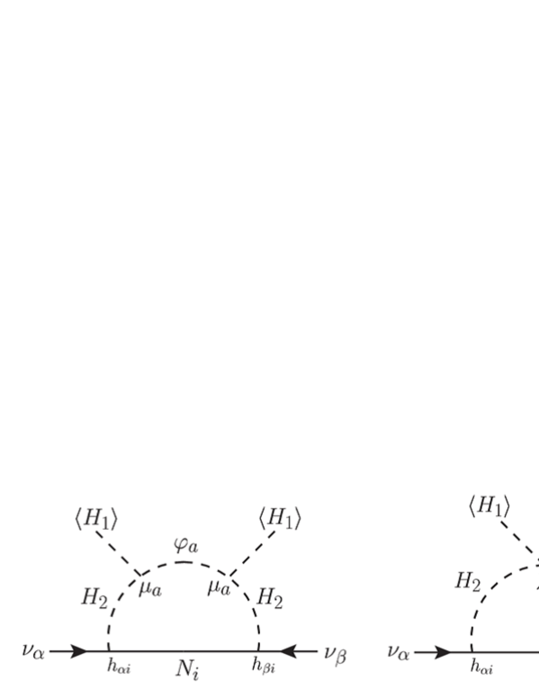
Figure 1: One-loop diagrams which contribute to the neutrino mass generation. The left diagram generates neutrino masses in the present model. The dimensionful coupling $\mu_{a}$ is defined as $\mu_{1}=\frac{\mu}{\sqrt{2}}$ and $\mu_{2}=\frac{i\mu}{\sqrt{2}}$ by using $\mu$ in eq. (1). Right one is the diagram in the original model Ma:2006km .

In this diagram, $\varphi_{a}$ represents component fields of $S$ which are defined as $S=\frac{1}{\sqrt{2}}(\varphi_{1}+\varphi_{2})$. Their masses are found to be $\bar{m}_{1}^{2}=\tilde{m}_{S}^{2}+m_{S}^{2}$ and $\bar{m}_{2}^{2}=\tilde{m}_{S}^{2}-m_{S}^{2}$. Since $Z_{2}$ is considered as an exact symmetry, $\tilde{m}_{S}^{2}>m_{S}^{2}$ should be satisfied. If we assume the condition $\tilde{m}_{S}\gg m_{S},m_{2},m_{N_{i}}$ is satisfied, the neutrino mass induced through the diagram in Fig. 1 can be estimated as

$${\cal M}^{\nu}_{\alpha\beta}=\sum_{i=1}^{3}h_{\alpha i}h_{\beta i}\frac{\langle H_{1}\rangle^{2}}{8\pi^{2}}\frac{m_{S}^{2}\mu^{2}}{\tilde{m}_{S}^{4}}\frac{m_{N_{i}}}{m_{H_{2}}^{2}-m_{N_{i}}^{2}}\left(1+\frac{m_{N_{i}}^{2}}{m_{H_{2}}^{2}-m_{N_{i}}^{2}}\ln\frac{m_{N_{i}}^{2}}{m_{H_{2}}^{2}}\right),$$ (2)

where $m_{H_{2}}^{2}=m_{2}^{2}+(\lambda_{3}+\lambda_{4})\langle H_{1}\rangle^{2}$. It is equivalent to the neutrino mass formula in the original model if $\frac{m_{S}^{2}\mu^{2}}{\tilde{m}_{S}^{4}}$ is identified with the coupling constant $\lambda_{5}$ for a $(H_{2}^{\dagger}H_{1})^{2}$ term.

This correspondence might be found in an effective theory obtained at energy regions smaller than $\tilde{m}_{S}$ by integrating out $S$. The origin of small $\lambda_{5}$ which is the key nature to explain the smallness of the neutrino masses is now translated to the hierarchy problem between $\mu$, $m_{S}$ and $\tilde{m}_{S}$ in this extension. If we leave the origin of this hierarchy to a complete theory at high energy regions, all the neutrino masses, the DM abundance and the baryon number asymmetry could be also explained in this extended model at TeV regions just as in the same way discussed in the previous articles Kashiwase:2012xd . Following the results obtained in these studies, the value of $\frac{m_{S}^{2}\mu^{2}}{\tilde{m}_{S}^{2}}$ could be constrained by the simultaneous explanation of these.

III Inflation due to the complex scalar $S$

We consider an inflation scenario which could work even for sub-Plankian values of $S$, following proposal in McDonald:2014oza . It is possible as long as the existence of specific nonrenormalizable terms is assumed in the potential for $S$. As such a potential, we suppose that the complex scalar $S$ has $Z_{2}$ invariant additional terms such as

$$V =c_{1}\frac{(S^{\dagger}S)^{n}}{M_{\rm pl}^{2n-4}}\left[1+c_{2}\left\{\left(\frac{S}{M_{\rm pl}}\right)^{2m}\exp\left(i\frac{S^{\dagger}S}{\Lambda^{2}}\right)+\left(\frac{S^{\dagger}}{M_{\rm pl}}\right)^{2m}\exp\left(-i\frac{S^{\dagger}S}{\Lambda^{2}}\right)\right\}\right],$$

$$=c_{1}\frac{\varphi^{2n}}{2^{n}M_{\rm pl}^{2n-4}}\left[1+2c_{2}\left(\frac{\varphi}{\sqrt{2}M_{\rm pl}}\right)^{2m}\cos\left(\frac{\varphi^{2}}{2\Lambda^{2}}+2m\theta\right)\right],$$ (3)

where both $n$ and $m$ are positive integers and $M_{\rm pl}$ is the reduced Planck mass. Here we assume the condition $\Lambda\ll\varphi\ll M_{\rm pl}$. We use the polar coordinate expression $S=\frac{\varphi}{\sqrt{2}}e^{i\theta}$ in the second equality of eq. (3).

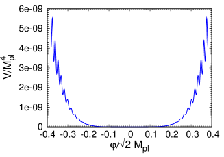
Figure 2: The left panel shows the potential $V$ defined by $n=3$ and $m=1$. Other Parameters in $V$ are fixed as $c_{1}=1.65\times 10^{-6}$, $c_{2}=0.7$ and $\Lambda/M_{\rm pl}=0.04$. The right panel depicts the time evolution of the inflaton in the $(\frac{\varphi_{1}}{\sqrt{2}M_{\rm pl}},\frac{\varphi_{2}}{\sqrt{2}M_{\rm pl}})$ plane for the potential $V$ shown in the left panel. $\varphi$ is related to $\varphi_{1,2}$ by $\varphi^{2}=\varphi_{1}^{2}+\varphi_{2}^{2}$.

In the left panel of Fig. 2, we show a typical shape of the potential as a function of $\varphi$ for a fixed $\theta$. We assume that inflaton moves along this local minimum. In the right panel of Fig. 2, we show an example for the evolution of the inflaton in the $(\frac{\varphi_{1}}{\sqrt{2}M_{\rm pl}},\frac{\varphi_{2}}{\sqrt{2}M_{\rm pl}})$ plane. In this calculation, we assume that $\varphi_{1,2}$ initially stay at the local minimum. The figure shows that the inflaton evolves along an aperiodic circle. During this evolution, the value of inflaton changes by an amount larger than the Planck scale for the small change of $\varphi$ in the sub-Planckian range. From this figure, we find that the single inflaton scenario could be realized in this model as long as we assume that the conditions mentioned above are satisfied and also the fields $\varphi_{1,2}$ start to evolve from a local minimum.

In order to see the feature of the inflation in this model, we calculate the quantities which characterize the inflation, that is, the e-foldings $N$, the spectral index $n_{s}$ and the tensor-to-scalar ratio $r$ (See more details in Budhi:2014gxa ). In Table 1, we show typical examples which are calculated numerically for different values for the model parameters $c_{1}$, $c_{2}$ and $\Lambda$. These examples suggest that sufficiently large e-foldings such as $N_{\ast}=50$ - 60 could be realized as long as $\Lambda\ll\varphi_{\ast}$ is satisfied even for the sub-Planckian inflaton value $\varphi_{\ast}<M_{\rm pl}$. The predicted values of $n_{s}$ and $r$ are also listed in each case. In Fig. 3, we plot the predicted points in the $(n_{s},r)$ plane for $N_{\ast}=50$ - 60 in the cases A, B and C given in Table 1. As we can see from this figure, both cases A and B which were favored by BICEP2 Ade:2014xna have been excluded by the recent Planck data Ade:2015lrj . On the other hand, the case C is in the region of the 95% CL due to the Planck results. We will examine the viable region in this model more extensively in pre .

Table 1: The spectral index and the tensor-to-scalar ratio for typical examples of three parameters in the potential (3) defined by $n=3$ and $m=1$. These model parameters are fixed to realize the observed value for the scalar perturbation amplitude $\Delta_{\cal R}^{2}$ at $k_{*}=0.002$ Mpc^-1.

	$c_{1}$	$c_{2}$	$\frac{\Lambda}{M_{\rm pl}}$	$\frac{\varphi_{*}}{\sqrt{2}M_{\rm pl}}$	$N_{*}$	$n_{s}$	$r$
A	$1.66\times 10^{-6}$	0.7	0.04	0.378	59.0	0.971	0.107
	$2.04\times 10^{-6}$	0.7	0.04	0.371	54.2	0.968	0.119
	$2.42\times 10^{-6}$	0.7	0.04	0.366	49.1	0.965	0.131
B	$0.257$	6.0	0.002	0.0512	60.4	0.969	0.124
	$0.305$	6.0	0.002	0.0505	55.0	0.966	0.136
	$0.364$	6.0	0.002	0.0498	50.0	0.962	0.149
C	$0.82\times 10^{-6}$	1.4	0.05	0.425	66.6	0.966	0.066
	$1.52\times 10^{-6}$	1.4	0.05	0.406	48.3	0.960	0.101

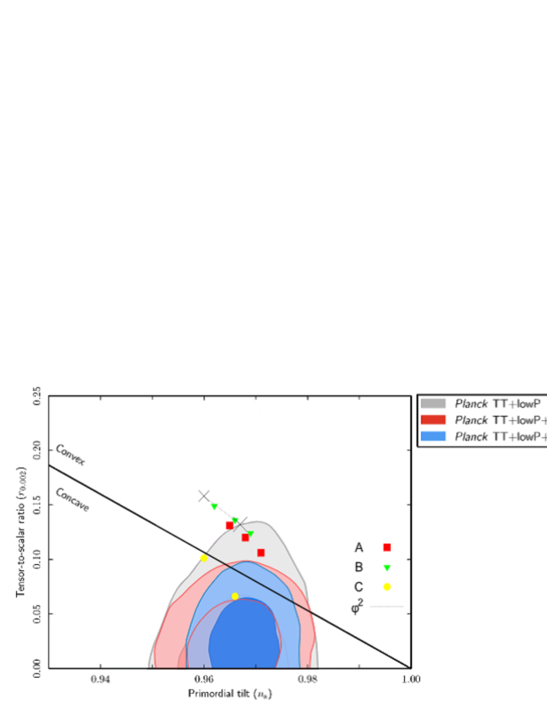
Figure 3: Predicted values of $(n_{s},r)$ for several parameter sets $(c_{2},\frac{\Lambda}{M_{\rm pl}})$ given in Table 1. A dotted line represents the prediction by the quadratic chaotic inflation model and the crosses correspond to the points for $N_{\ast}=50$ and 60. Contours given as Fig. 54 in Planck Collaboration XX Ade:2015lrj are used here.

IV Reheating after the end of inflation

In this model, the Universe could be reheated up through inflaton decay after the end of inflation. Since $\tilde{m}_{S}\gg m_{S}$ is assumed to be satisfied here, the reheating temperature realized through this process could be estimated as

$$T_{R}\simeq 1.6\times 10^{8}\left(\frac{|\lambda_{5}|}{10^{-6}}\right)^{1/2}\left(\frac{\tilde{m}_{S}}{m_{S}}\right)\left(\frac{\tilde{m}_{S}}{10^{6}~{}{\rm GeV}}\right)^{1/2}~{}{\rm GeV}.$$ (4)

In this estimation, we take account of the constraint from the neutrino mass generation as discussed in the previous part. Here we also note that $|\lambda_{5}|$ should be larger than $O(10^{-6})$, which is imposed by the present bound of DM direct search since we suppose that the lightest neutral component of $H_{2}$ is DM and its mass is $\sim 1$ TeV Kashiwase:2012xd . We find that the reheating temperature could take values in a wide range such as $10^{5}{\rm GeV}~{}{{}^{<}_{\sim}}~{}T_{R}~{}{{}^{<}_{\sim}}~{}10^{15}~{}{\rm GeV}$ depending on a value of $\tilde{m}_{S}$. This temperature is high enough to produce thermal right-handed neutrinos in the present model since the masses of right-handed neutrinos are assumed to be of $O(1)$ TeV. If the right-handed neutrino masses are sufficiently degenerate, the baryon number asymmetry could be generated through the resonant leptogenesis as discussed in Kashiwase:2012xd . Right-handed neutrinos need not to be light but they could have large mass such as $O(10^{9})$ GeV in a consistent way with this neutrino mass model Kashiwase:2012xd . Even in that case, eq. (4) shows that the reheating temperature could be high enough for leptogenesis to work well without the resonant effect.

V conclusion

We have considered an extension of the radiative seesaw model with a complex singlet scalar to realize the inflation of the Universe keeping favorable features of the original model, that is, the simultaneous explanation of the small neutrino masses, the DM abundance and the baryon number asymmetry in the Universe. This singlet scalar plays a crucial role not only for inflation but also for the small neutrino mass generation. In this scenario, the inflaton trajectory follows an aperiodic circle during the inflation. This feature makes it possible that sub-Planckian values of the relevant field induce trans-Planckian change of the inflaton value which is needed for the sufficient e-foldings. The model could be free from the serious problem caused by trans-Planckian field values. Both the spectral index $n_{s}$ and the tensor-to-scalar ratio $r$ could have values which are favorable from the recent CMB observations. The roughly estimated reheating temperature could be high enough for leptogenesis.

- (1) ATLAS Collaboration, G. Aad, el al., Phys. Lett. B716 (2012) 1; CMS Collaboration, S. Chatrchyan, el al., Phys. Lett. B716 (2012) 30.
- (2) Super-Kamiokande Collaboration, Y. Fukuda, et al., Phys. Rev. Lett. 81 (1998) 1562; SNO Collaboration, Q. R .Ahmad, et al., Phys. Rev. Lett. 89 (2002) 011301; KamLAND Collaboration, K. Eguchi, et al., Phys. Rev. Lett. 90 (2003) 021802; K2K Collaboration, M. H. Ahn, et al., Phys. Rev. Lett. 90 (2003) 041801;
- (3) T2K Collaboration, K. Abe, et al., Phys. Rev. Lett. 107 (2011) 041801; Double Chooz Collaboration, Y. Abe, et al., Phys. Rev. Lett. 108 (2012) 131801; RENO Collaboration, J. K. Ahn, et al., Phys. Rev. Lett. 108 (2012) 191802; The Daya Bay Collaboration, F. E. An, et al., Phys. Rev. Lett. 108 (2012) 171803.
- (4) WMAP Collaboration, D. N. Spergel, et al., Astrophys. J. 148 (2003) 175; SDSS Collaboration, M. Tegmark, et al., Phys. Rev. D69 (2004) 103501.
- (5) A. Riotto and M. Trodden, Ann. Rev. Nucl. Part. Sci. 49 (1999) 35; W. Bernreuther, Lect. Notes Phys. 591 (2002) 237; M. Dine and A. Kusenko, Rev. Mod. Phys. 76 (2003) 1.
- (6) E. Ma, Phys. Rev. D 73, 077301 (2006).
- (7) S. Kashiwase and D. Suematsu, Phys. Rev. D 86, 053001 (2012); S. Kashiwase and D. Suematsu, Eur. Phys. J. C 73, 2484 (2013).
- (8) P. A. R. Ade et al. [Planck Collaboration], arXiv:1502.02114 [astro-ph.CO].
- (9) R. H. S. Budhi, S. Kashiwase and D. Suematsu, Phys. Rev. D 90 (2014) 11, 113013.
- (10) J. McDonald, JCAP 1409 (2014) 09, 027.
- (11) P. A. R. Ade et al. [BICEP2 Collaboration], Phys. Rev. Lett. 112 (2014) 24, 241101.
- (12) Romy H. S. Budhi, S. Kashiwase and Daijiro Suematsu, in preparation.