Modeling Networks with
a Growing Feature-Structure

Abstract

We present a new network model accounting for multidimensional assortativity. Each node is characterized by a number of features and the probability of a link between two nodes depends on common features. We do not fix a priori the total number of possible features. The bipartite network of the nodes and the features evolves according to a stochastic dynamics that depends on three parameters that respectively regulate the preferential attachment in the transmission of the features to the nodes, the number of new features per node, and the power-law behavior of the total number of observed features. Our model also takes into account a mechanism of triadic closure. We provide theoretical results and statistical estimators for the parameters of the model. We validate our approach by means of simulations and an empirical analysis of a network of scientific collaborations.

keyword: complex network, bipartite network, assortativity, homophily, preferential attachment, triadic closure.

1 Introduction

Many complex systems are often described by means of a network of interacting components, i.e. a set of nodes connected by links [6, 15, 18, 30, 61]. A large number of scientific fields involve the study of networks in some form: networks have been used to analyze interpersonal social relationships, communication systems, international trade, financial systems, co-authorships and citations, protein interaction patterns, and much more. Therefore, formal stochastic models and statistical techniques for the analysis of network data have emerged as a major topic of interest in diverse areas of study. The distribution of the number of node’s connections is well approximated by a power-law in many contexts and preferential attachment is generally accepted as the simplest mechanism that can reproduce such a distribution [3, 4]. This basic mechanism, however, is only one of the many forces that can contribute to shape the evolution of complex networks. For instance, a social network having power-law degree distribution is an exception rather than the rule. In particular, preferential attachment is not able to reproduce the formation of social groups, or communities, and the composition of social circles. Assortativity (or assortative mixing), called homophily in social networks, is defined as the prevalence of network-links between nodes that are similar to each other in some respect. Network theorists often analyze assortativity in terms of a node’s degree [2, 47, 52, 53]. Moreover, a large body of research in sociology and, more recently, in economics, confirms the presence of a multidimensional assortativity in socio-economic networks: homophily, along the lines of race and ethnicity, age and sex, education, professional background and occupation, shapes complex networks such as friendship, marriage, teamwork, co-membership, exchange and communication networks [8, 9, 11, 14, 16, 18, 19, 22, 29, 32, 34, 35, 40, 41, 42, 44, 54, 60]. The assortativity property has been also studied in citation networks: for instance, in [13] authors analyze the citations among papers (the nodes of the network) published in journals of the American Physical Society with respect to their PACS classification codes, that represent the different research sub-fields. In formal models assortativity is typically represented by partitioning nodes into different classes (also called groups, clusters, or types) related to some (observable or unobservable) features [1, 13, 20, 23, 24, 25, 26, 27, 33, 37, 49, 58]. The assumption that each node can belong only to a single class and/or the fact that the number of classes is finite and fixed a priori as well as the number of the possible features restrict their applicability.

We contribute to this growing body of literature by introducing a new stochastic model accounting for multidimensional assortativity. The study of networks of papers, such as co-authorship or citation networks [5, 13, 21, 48], is a particularly suitable application of our model as the generative processes of features and links are consistent with the basic aspects of the model: first, it is a growing network process where nodes appear in chronological order and do not exit; second, the links are established at the entrance of the nodes and are unchangeable along time; third, each node exhibits some features (for example, key-words, main topics, etc.) that are unchangeable during time; finally, the set of the features grows in time and the evolution of the nodes-features structure is interesting exactly as the process of the link-creation among the nodes. Indeed, the description of both phenomena is very important for the understanding of the diffusion process of ideas and discoveries inside a certain research field and among different research fields. Anyway, as we will discuss at the end of this paper, our model can be easily modified and/or enriched in order to get variants that better fit networks of a different type.

In particular, besides the link-creation mechanism, our model provides a stochastic dynamics for the evolution of the features. Differently from the above quoted works (see, for instance, the model in [37] and the related discussion about the selection problem for the dimension of the feature-space), we do not fix a priori the total number of possible features but we allow the number of observed features to grow in time. The bipartite nodes-features network (i.e. the surrounding context) grows according to a stochastic model that depends on three parameters that respectively regulate the preferential attachment in the transmission of the features to the nodes, the number of new features per node, and the power-law behavior of the total number of observed features. Concerning this point, the present paper may be considered as a companion article to [12]. Indeed, both of them provide an evolving dynamics for the feature-structure, but they also show some differences. The main issue is that here we introduce a parameter that tunes the preferential attachment in the transmission of the features to the nodes; while in [12] authors only consider a preferential attachment rule. Moreover, in that paper a random “fitness” parameter which determines the node’s ability to transmit its own features to other nodes (see also [7]) is attached to each node; while here we do not take into account fitness parameters for nodes.

Coming from a structural approach, differently from other models which concentrate only on assortativity [17, 45, 51, 56], our model also accounts for the principle, known as triadic closure or transitivity, according to which, if A is a neighbor of B and B is a neighbor of C, then A and C have a high chance to be neighbors. This principle is widely supported on the empirical ground and it is at the basis of many generative network models [10, 18, 22, 28, 31, 35, 41, 43, 46, 50, 55, 57, 59]. It is worthwhile to note that the expression “triadic closure” conceptually refers to a link-formation process not depending on the features of the nodes that get attached. However, also assortativity can naturally induce closed triplets in the network and hence evaluating assortativity and triadic closure separately sometimes may be not easy. (For a further discussion on this issue, we refer to the next Section 5.) Anyway models based on both mechanisms produce more realistic networks.

The paper is structured as follows. In Section 2 we describe the basic assumptions of our model and the notation used throughout the paper. In Section 3 we present our stochastic model, that involves a dynamics for the bipartite network of nodes-features and the mechanism underlying the formation of the unipartite (i.e. node-node) network. In Section 4 we illustrate some theoretical results and we carefully explain the meaning of each parameter inside our model. In Section 5 we show and discuss some statistical tools in order to estimate the model parameters from the data. In Section 6 we provide a number of simulations in order to point out the functioning of the model parameters and the ability of the proposed estimation tools. Section 7 deals with an application of our model and instruments to a co-authorship network. Finally, in Section 8 we give our conclusions and discuss some future developments. The paper is enriched by an Appendix that contains a theorem and its proof, and supplementary simulation results.

2 Preliminaries

We assume new nodes sequentially join the network so that node $i$ represents the one that comes into the network at time step $i$. Each node shows a finite number of features, that can be of different kinds (key-words, main topics, spatial/geographical contexts, profile, etc.), and different nodes can share the same features. It is worthwhile to note that we do not specify a priori the total number of possible features but we allow the number of observed features to increase along time. On its arrival, each new node links to some nodes already present in the system. Firstly, links are created according to probabilities that depend on the number of common features (multidimensional assortativity). Then additional links can be established by means of common neighbors, inducing the closure of some triangles (triadic closure). We consider the connections as undirected, non-breakable and we omit self-loops (i.e. edges of type $(i,i)$). In particular, this means that connections are mutual or the direction is naturally predefined (for instance, only citations from newer to older nodes are possible). We denote the adjacency matrix (symmetric by assumption) by $A$, so that $A_{i,j}=1$ when there exists a link between nodes $i$ and $j$, $A_{i,j}=0$ otherwise. We set

$${\mathcal{V}}_{j}(i)=\{j^{\prime}=1,\dots,i:A_{j,j^{\prime}}=1\}$$

to be the set of node $j$’s neighbors at time step $i$ (after the arrival of $i$).

We denote by $F$ the binary bipartite network where each row $F_{i}$ represents the features of node $i$: $F_{i,k}=1$ if node $i$ has feature $k$, $F_{i,k}=0$ otherwise. It represents the surrounding context in which the nodes interact. We assume that each $F_{i}$ is unchangeable during time. We take $F$ left-ordered: this means that in the first row the columns for which $F_{1,k}=1$ are grouped on the left and hence, if the first node has $N_{1}$ features, then the columns of $F$ with index $k\in\{1,\dots,N_{1}\}$ represent these features. The second node could have some features in common with the first node (those corresponding to indices $k$ such that $k=1,\dots,N_{1}$ and $F_{2,k}=1$) and some, say $N_{2}$, new features. The latter are grouped on the right of the set for which $F_{1,k}=1$, i.e., the columns of $F$ with index $k\in\{N_{1}+1,\dots,N_{2}\}$ represent the new features brought by the second node. This grouping structure persists throughout the matrix $F$ and we define $L_{n}=\sum_{i=1}^{n}N_{i}$, i.e.

$$\begin{split}L_{n}=\hbox{overall number of different observed features for the first }n\hbox{ nodes}.\end{split}$$ (2.1)

Here is an example of a $F$ matrix with $n=3$ nodes:

$$F=\left(\begin{array}[]{cccccccccccc}\pagecolor{gray!20}1&\pagecolor{gray!20}1&\pagecolor{gray!20}1&0&0&0&0&0\\ 1&0&1&\pagecolor{gray!20}1&\pagecolor{gray!20}1&0&0&0\\ 0&1&1&1&0&\pagecolor{gray!20}1&\pagecolor{gray!20}1&\pagecolor{gray!20}1\\ \end{array}\right).$$

In gray we show the new features brought by each node (in the example $N_{1}=3$, $N_{2}=2$, $N_{3}=3$ and so $L_{1}=3,L_{2}=5,L_{3}=8$). Observe that, for every node $i$, the $i$-th row contains 1 for all the columns with indices $k\in\{L_{i-1}+1,\dots,L_{i}\}$ (they represent the new features brought by $i$). Moreover, some elements of the columns with indices $k\in\{1,\dots,L_{i-1}\}$ are also $1$ (features brought by previous nodes adopted by node $i$).

3 The model

Fix $\alpha>0$, $\beta\in[0,1]$, $\delta\in[0,1]$, $p\in[0,1]$ and let $\Phi:{\mathbb{R}}\to[0,1]$ be an increasing function. The dynamics is the following. Node 1 arrives and shows $N_{1}$ features, where $N_{1}$ is Poi$(\alpha)$-distributed (the symbol Poi$(\alpha)$ denotes the Poisson distribution with mean $\alpha$). Then, for each $i\geq 2$,

• Feature-structure dynamics: Node $i$ arrives and shows a number of features as follows:

  • Node $i$ exhibits some of the “old” features brought by the previous nodes $1,\dots,i-1$: more precisely, each feature $k\in\{1,\dots,L_{i-1}\}$ is, independently of the others, possessed by node $i$ with probability (that we call “inclusion-probability”)

    $$P_{i}(k)=\delta\frac{1}{2}+(1-\delta)\frac{\sum_{j=1}^{i-1}F_{j,k}}{i}\,,$$ (3.1)

    where $F_{j,k}=1$ if node $j$ shows feature $k$ and $F_{j,k}=0$ otherwise.

  • Node $i$ also shows $N_{i}$ “new” features, where $N_{i}$ is Poi$(\lambda_{i})$-distributed with

    $$\lambda_{i}=\frac{\alpha}{i^{1-\beta}}.$$ (3.2)

  ($N_{i}$ is independent of $N_{1},\dots,N_{i-1}$ and of the exhibited “old” features.)
  The matrix element $F_{i,k}$ is set equal to $1$ if node $i$ has feature $k$ and equal to zero otherwise.

• Network construction: On its arrival, node $i$ determines a set ${\mathcal{L}}_{i}$ of neighbors among the nodes already present in the network (so that we set $A_{i,j}=A_{j,i}=1$ for each $j\in{\mathcal{L}}_{i}$) as follows:

  • (First phase) First, a set ${\mathcal{L}}_{i}^{*}$ of neighbors of node $i$ is established on the basis of the features shown. Each node $j$ already present in the network (i.e. $1\leq j\leq i-1$) is included in ${\mathcal{L}}_{i}^{*}$, independently of the others, with probability $\Phi(S_{i,j})$, where

    $$S_{i,j}=\sum_{k=1}^{L_{i}}F_{i,k}F_{j,k}.$$ (3.3)

    is the number of features that $i$ and $j$ have in common.

  • (Second phase) Then some extra neighbors are added to ${\mathcal{L}}_{i}$ on the basis of common neighbors. For every node $j\in\{1,\dots,i-1\}\setminus{\mathcal{L}}_{i}^{*}$, each node $j^{\prime}\in{\mathcal{V}}_{j}(i-1)\cap{\mathcal{L}}_{i}^{*}$ (i.e. each neighbor that $i$ and $j$ currently share) can induce, independently of the others, the additional link $(i,j)$ with probability $p$.

4 Meaning of the model parameters and some results

We now illustrate the meaning of the model parameters and some mathematical results regarding our model.

4.1 The parameters $\alpha$ and $\beta$

Let us start with $\alpha$ and $\beta$. The main effect of $\beta$ is to regulate the asymptotic behavior of the random variable $L_{n}$ defined in (2.1) as a function of $n$. In particular, $\beta>0$ is the power-law exponent of $L_{n}$. The main effect of $\alpha$ is the following: the larger $\alpha$, the larger the total number of new features brought by a node. It is worth to note that $\beta$ fits the asymptotic behavior of $L_{n}$ and then, separately, $\alpha$ fits the number of new observed features per node. (In Section 6.1 we will discuss more deeply this fact.) More precisely, we prove (see the Appendix) the following asymptotic behaviors:

• for $\beta=0$, we have a logarithmic behavior of $L_{n}$, that is ${L_{n}}/{\ln(n)}\stackrel{{\scriptstyle a.s.}}{{\longrightarrow}}\alpha$;

• for $\beta\in(0,1]$, we obtain a power-law behavior, i.e. ${L_{n}}/{n^{\beta}}\stackrel{{\scriptstyle a.s.}}{{\longrightarrow}}{\alpha}/{\beta}$.

4.2 The parameter $\delta$

The parameter $\delta$ tunes the phenomenon of preferential attachment in the spreading process of features among nodes. The value $\delta=0$ corresponds to the “pure preferential attachment case”: the larger the weight of a feature $k$ at time step $i-1$ (given by the numerator of the second element in (3.1), i.e., the total number of nodes that exhibit it until time step $i-1$), the greater the probability that $k$ will be shown by the future node $i$. The value $\delta=1$ corresponds to the “pure i.i.d. case” with inclusion probability equal to $1/2$: a node includes each feature with probability $1/2$ independently of the other nodes and the other features. When $\delta\in(0,1)$, we have a mixture of the two cases above: the smaller $\delta$, the more significant is the role played by preferential attachment in the transmission of the features to new nodes.

4.3 The function $\Phi$ and the parameter $p$

According to our model, when a new node enters the system, it links to some (possibly zero, one, or more) old nodes by means of the two phases network construction described in Section 3. In the first phase, a new node $i$ connects itself to some of the old nodes according to a probability depending on its own features and the ones of the others. The function $\Phi$ relates the “first-phase link-probability” of $i$ to $j$ (with $1\leq j\leq i-1$) to their “similarity” $S_{i,j}$ defined by (3.3). Since $\Phi$ is assumed to be an increasing function, a higher number of common features between nodes $i$ and $j$ induces a larger probability for them to connect (akin the principle of assortativity). For instance, we can take the generalization of the logistic function, i.e. the sigmoid function

$$\Phi(s)=\frac{1}{1+e^{K(\vartheta-s)}}\qquad\hbox{with }K>0,\,\vartheta\in\mathbb{R}.$$ (4.1)

The sigmoid function smoothly increases (from $0$ to $1$) around a threshold $\vartheta$, while $K$ controls its smoothness: the bigger $K$, the steeper the sigmoid. In particular, $K=1$ and $\vartheta=0$ give the logistic function and, for $K\to+\infty$, $\Phi$ approaches to a step function equal to $1$ or $0$, if the variable $s$ is respectively greater or smaller than $\vartheta$ (in our model, $\vartheta\geq 0$ means that the links are established deterministically based on whether the two involved nodes have, or not, a similarity bigger than $\vartheta$). In the second phase, node $i$ can connect to some of the nodes discarded in the first phase by means of common neighbors (triadic closure). The parameter $p$ regulates this phenomenon. Indeed, it represents the probability that a node causes a link between two of its neighbors. More precisely, in the second phase, the probability of having a link between node $i$ and a node $j\in\{1,\dots,i-1\}\setminus{\mathcal{L}}_{i}^{*}$ is $\left[1-(1-p)^{C_{i,j}}\right]$, where $C_{i,j}=\mbox{card}\big{(}{\mathcal{V}}_{j}(i-1)\cap{\mathcal{L}}_{i}^{*}\big{)}$ is the number of common neighbors of $i$ and $j$ after the first phase. Consequently, the “second-phase link-probability” between a pair of nodes increases with respect to $p$ and the number of neighbors they share. The case $p=0$ corresponds to the case in which the connections only depend on the similarity among nodes. The case $p=1$ corresponds to the case in which the connection is automatically established when $C_{i,j}>0$.

5 Estimation of the model parameters

In this section we illustrate how to estimate the model parameters from the data.

Suppose we can observe the values of $F_{1},\dots,F_{n}$, i.e. $n$ rows of the matrix $F$, where $n$ is the number of observed nodes. From the asymptotic behavior of $L_{n}$, we get that $\ln(L_{n})/\ln(n)$ is a strongly consistent estimator for $\beta$, hence we can use the slope $\widehat{\beta}$ of the regression line in the log-log plot (of $L_{n}$ as a function of $n$) as an estimate for $\beta$.

After computing $\widehat{\beta}$, we can estimate $\alpha$ as:

$$\begin{split}\widehat{\alpha}&=\widehat{\gamma}\qquad\hbox{when }\widehat{\beta}=0\\ \widehat{\alpha}&={\widehat{\beta}}\,\widehat{\gamma}\qquad\hbox{when }0<\widehat{\beta}\leq 1,\end{split}$$ (5.1)

where $\widehat{\gamma}$ is the slope of the regression line in the plot $\big{(}\ln(n),L_{n}\big{)}$ or in the plot $\big{(}n^{\widehat{\beta}},L_{n}\big{)}$ according to whether $\widehat{\beta}=0$ or $\widehat{\beta}\in(0,1]$.

We can estimate $\delta$ by means of a maximum likelihood procedure. For this purpose, we now give a general expression of the probability of observing $F_{1}=f_{1},\dots,F_{n}=f_{n}$ given the parameters $\alpha,\beta$, and $\delta$.

The first row $F_{1}$ is simply identified by $L_{1}=N_{1}$ and so

$$\begin{split}P(F_{1}=f_{1})&=P(N_{1}=n_{1}=\mbox{card}\{k:f_{1,k}=1\})\\ &=\mbox{Poi}(\alpha)\{n_{1}\}=e^{-\alpha}\frac{\alpha^{n_{1}}}{n_{1}!}.\end{split}$$

Then the second row is identified by the values $F_{2,k}$, with $k=1,\dots,L_{1}=N_{1}$, and by $N_{2}$, so that

$$\begin{split}&P(F_{2}=f_{2}|F_{1})=\\ &P(F_{2,k}=f_{2,k}\,\hbox{for }k=1,\dots,L_{1},\,N_{2}=n_{2}=\mbox{card}\{k>L_{1}:f_{2,k}=1\}|F_{1})=\\ &\prod_{k=1}^{L_{1}}P_{2}(k)^{f_{2,k}}(1-P_{2}(k))^{1-f_{2,k}}\times\mbox{Poi}(\lambda_{2})\{n_{2}\},\end{split}$$

where $P_{2}(k)$ is defined in (3.1) and $\lambda_{2}$ is defined in (3.2). The general formula is

$$\begin{split}&P(F_{i}=f_{i}|F_{1},\dots,F_{i-1})=\\ &P\left(F_{i,k}=f_{i,k}\,\hbox{for }k=1,\dots,L_{i-1},\,\right.\\ &\quad\quad\left.N_{i}=n_{i}=\mbox{card}\{k>L_{i-1}:f_{i,k}=1\}|F_{1},\dots,F_{i-1}\right)=\\ &\prod_{k=1}^{L_{i-1}}P_{i}(k)^{f_{i,k}}(1-P_{i}(k))^{1-f_{i,k}}\times\mbox{Poi}(\lambda_{i})\{n_{i}\},\end{split}$$

where $P_{i}(k)$ is defined in (3.1) and $\lambda_{i}$ is defined in (3.2). Thus, for $n$ nodes, we can write a formula for the probability of observing $F_{1}=f_{1},\dots,F_{n}=f_{n}$:

$$\begin{split}&P(F_{1}=f_{1},\dots,F_{n}=f_{n})=\\ &P(F_{1}=f_{1})\prod_{i=2}^{n}P(F_{i}=f_{i}|F_{1},\dots,F_{i-1}).\end{split}$$ (5.2)

Therefore, we look for $\widehat{\delta}$ that maximizes the likelihood function, i.e. the quantity $P(F_{1}=f_{1},\dots,F_{n}=f_{n})$ as a function of $\delta$ (given the observed vectors $f_{i}$). Since some factors do not depend on $\delta$, we can simplify the function to be maximized as

$$\prod_{i=2}^{n}\prod_{k=1}^{L_{i-1}}P_{i}(k)^{f_{i,k}}(1-P_{i}(k))^{1-f_{i,k}},$$ (5.3)

or, equivalently, passing to the logarithm, as

$$\sum_{i=2}^{n}\sum_{k=1}^{L_{i-1}}f_{i,k}\ln\big{(}P_{i}(k)\big{)}+(1-f_{i,k})\ln\big{(}1-P_{i}(k)\big{)}.$$ (5.4)

Now, suppose that we are also allowed to observe the adjacency matrix $A=(A_{i,j})_{1\leq i,j\leq n}$ (meaning the final adjacency matrix after the arrival of all the $n$ observed nodes and the formation of all their links) and to know which are the links that each of the $n$ observed nodes formed only by means of the previously described first phase (i.e. only due to assortativity). Denote by $A^{\prime}=(A^{\prime}_{i,j})_{1\leq i,j\leq n}$ the adjacency matrix collecting them. Then, if we decide to model the function $\Phi$ as in (4.1), we can choose $K$, $\vartheta$, and $p$, in order to fit some properties of the observed matrices $A^{\prime}$ and $A$. For instance, if $\ell$ is the number of observed (undirected) links in matrix $A^{\prime}$ (i.e. only due to the first phase of network construction) and

$$f^{*}=\frac{\hbox{observed number of linked (in $A^{\prime}$) pairs of nodes with }s^{*}\,\hbox{ features in common}}{\hbox{observed number of pairs of nodes with }s^{*}\,\hbox{ features in common}},$$

where $s^{*}$ is a fixed value that we choose, then we can determine $K>0$ and $\vartheta\in\mathbb{R}$ by solving (numerically) the following system of two equations:

$$\begin{split}&\Phi(s^{*})=\left(1+e^{K(\vartheta-s^{*})}\right)^{-1}=f^{*}\\[3.0pt] &E\left[\sum_{i,j:2\leq i\leq n,1\leq j\leq i-1}A^{\prime}_{i,j}\right]=\sum_{i=2}^{n}\sum_{j=1}^{i-1}\Phi\left(S_{i,j}\right)=\\ &\sum_{i=2}^{n}\sum_{j=1}^{i-1}\left(1+e^{K(\vartheta-s^{*})+K(s^{*}-\sum_{k=1}^{L_{i}}F_{i,k}F_{j,k})}\right)^{-1}=\ell.\end{split}$$ (5.5)

By means of the first equation, we fit the probability that a pair of nodes with $s^{*}$ features in common establishes a link (during the first phase of network construction); while, by the second equation, we set the expected number of links in $A^{\prime}$ equal to the observed $\ell$. From the first equation, we get the quantity $K(\vartheta-s^{*})$, we then replace it in the second one in order to obtain $K$ and from this we get $\vartheta$. Note that this is not a proper estimation procedure, but rather a selection mechanism for $K$ and $\vartheta$ in order to fit some observed properties of the network. After that, we can estimate $p$ by means of a maximum likelihood procedure based on the observed matrices.

Some important remarks follow. If in the considered situation the formation of links only occur according to the first phase (i.e. as a result of the assortativity property), then we can set $p=0$ as in this case the presence of closed triplets is only caused by common features and the matrix $A$ coincides with $A^{\prime}$. Then we have no problem to implement the previous procedures for detecting all the model parameters. When we have both phases of network construction (i.e. $p>0$), the detection of $K,\vartheta$, and $p$ may generate some problems since the available data are typically $F$ and $A$, while, in order to implement the above procedure, we also need to observe $A^{\prime}$. When we cannot observe $A^{\prime}$, we may try to reconstruct it from $A$ in some consistent way, if it is possible for the considered application [38]. However, every empirical criterion used to distinguish between the two different types of links (the ones due to the first phase and the ones induced by the second phase), obviously has some degree of arbitrariness and it can be hard to understand the bias implied by it. An example of this problem can be found in [13] regarding a citation network. In the case no suitable criterion is found, we may try to select $K,\vartheta$, and $p$ in such a way that some properties of the adjacency matrix generated by the model are close to the observed one. Statistical procedures that integrate out unobserved variables (in this case, $A^{\prime}$) or expectation-maximization (EM) algorithms are also possible and they will be subject of future developments. Therefore, although assortativity and triadic closure are theoretically well separated concepts, in practice there are situations in which estimating them singly is not a simple task. However, their combination is often necessary in order to get models that produce realistic networks. The simulation of the model with the observed matrix $F$ and $p=0$ can be useful as a benchmark.

6 Simulations

In this section, we present a number of simulations performed following the dynamics for the features’ selection and links’ creation described in Section 3. We simulated the outcome for feature matrices and for unipartite networks of $1000$ nodes, on a sample of $100$ realizations. Regarding the feature-selection dynamics, we analyzed the resulting feature matrices (constructed as explained in Section 2) for different values of the model parameters $\alpha$, $\beta$, and $\delta$, responsible respectively of the number of new features per node, the asymptotic behavior of $L_{n}$ defined in (2.1), and the phenomenon of preferential attachment in the transmission of the features to new nodes. After that, we simulated the network construction taking $\Phi$ as in (4.1) and analyzed its properties for different values of $\delta$, $K$, and $p$, while $\vartheta$ is determined according to a certain number $\ell$ of (undirected) links due to the first phase of the unipartite network construction.

6.1 Simulations of the feature matrix and estimation of $\alpha,\,\beta$, and $\delta$

As said before, parameter $\alpha$ is responsible for the number of new features per node: the larger $\alpha$, the higher the number of new features per node. Concerning this, it is very important to stress that also the parameter $\beta$ affects the number of features per node, but the idea is that we select first $\beta$, in order to fit the asymptotic behavior of $L_{n}$, and then $\alpha$ in order to fit the number of new features per node.

In the first set of simulations we kept $\beta=0.5$ and $\delta=0.1$ fixed and we built the feature matrix for different values of $\alpha=3,\,8,\,13$. In Figure 1 we can see the shapes of the feature matrices (where colored points denote non-zero values, i.e. $1$) for the three different values of $\alpha$. It is immediate to see that the main difference among these matrices concerns the number of features: the total number of features is $185$ for $\alpha=3$, $533$ for $\alpha=8$, and $819$ for $\alpha=13$. Correspondingly, the mean number of new features per node (averaged over $100$ realizations) is about $0.19$ for $\alpha=3$, $0.49$ for $\alpha=8$, and $0.8$ for $\alpha=13$. The mean number of (total) adopted features per node (averaged over $100$ realizations) is about $19.99$ for $\alpha=3$, $52.66$ for $\alpha=8$, and $79.65$ for $\alpha=13$.

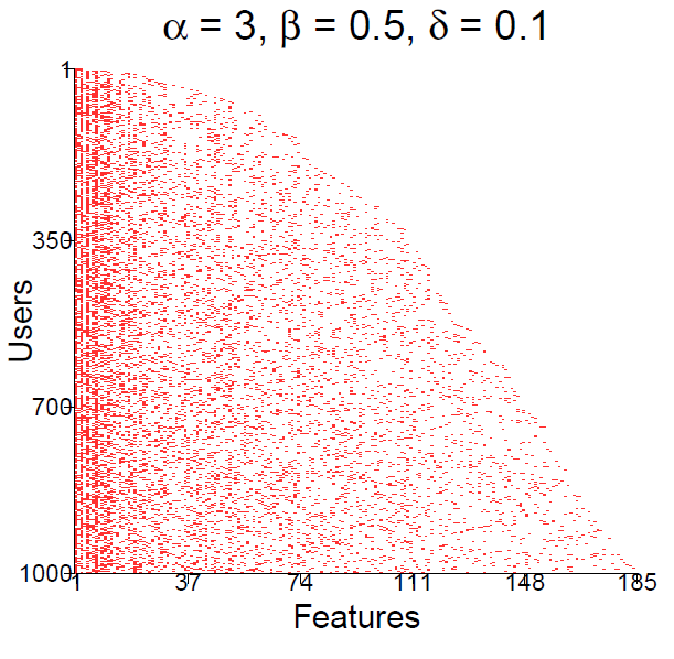
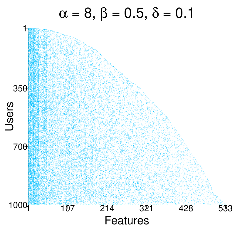
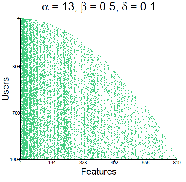
Figure 1: An example of features matrices for $n=1000$, $\beta=0.5$, $\delta=0.1$, and different values of $\alpha:3$ (left), $8$ (middle), $13$ (right). Colored points denote $1$ and white points denote $0$.

In Figure 2 we show the estimates for the different values of $\alpha$ (with $\beta=0.5$ and $\delta=0.1$ kept fixed).

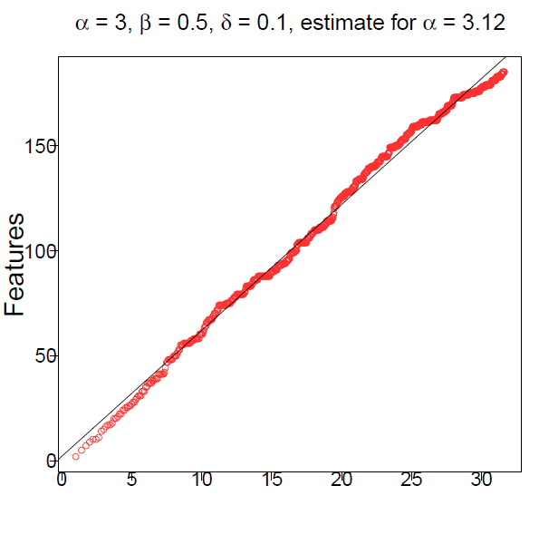
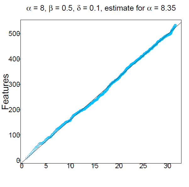
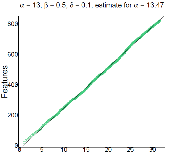
Figure 2: Estimates of $\alpha$ (when $\beta=0.5$ and $\delta=0.1$) obtained as the slope of the regression line in the plot of $L_{n}$ as a function of $n^{\beta}$. Different values of $\alpha:3$ (left), $8$ (middle), $13$ (right) are reported.

Parameter $\beta$ controls the asymptotic behavior of $L_{n}$. For this reason we plotted $L_{n}$ as a function of $n$ in a log-log scale, results are reported in Figure 3. In Figure 3 (a)-(b), we show the estimates for two different values of $\beta$ ($\beta=0.75$ and $\beta=1$), with $\alpha=3$ and $\delta=0.1$. In Figure 3 (c)-(d), we show the estimate of $\beta$, for $\beta=0.5$ and $\beta=0.75$, but for a different value of $\alpha$ ($\alpha=10$) in order to underline that $\alpha$ does not affect the power-law behavior of $L_{n}$ (obviously, the value of the estimate can be more or less accurate for different values of $\alpha$).

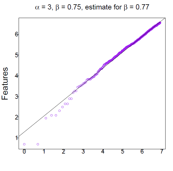
(a)

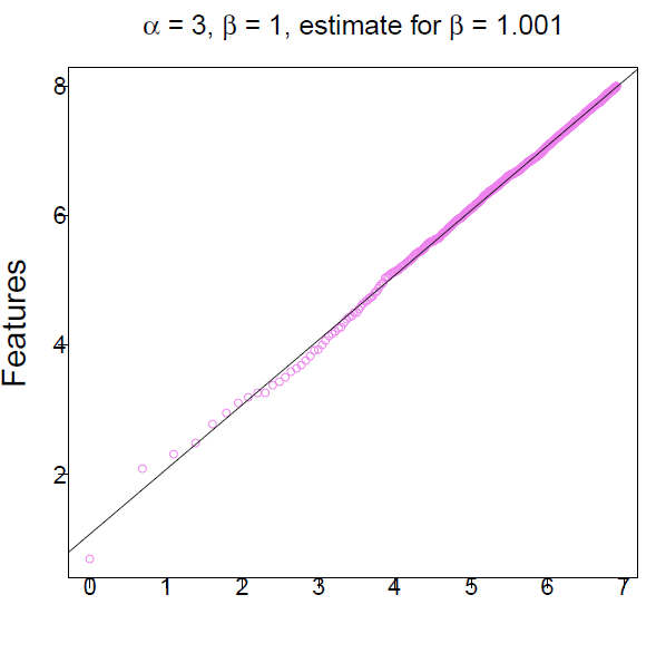
(b)

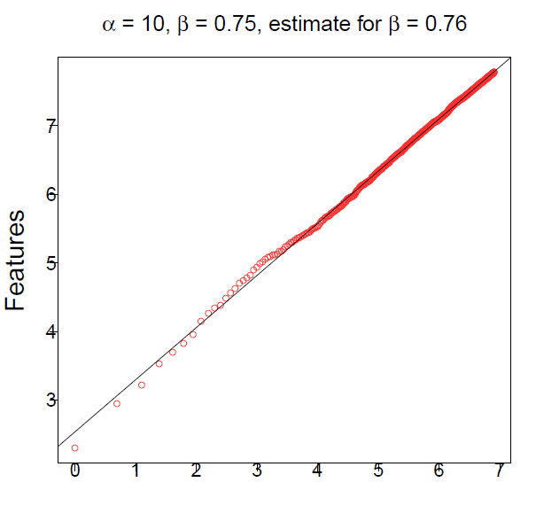
(c)

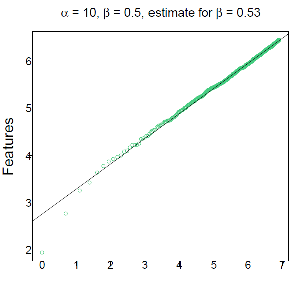
(d)

Figure 3: Estimates of $\beta$ obtained as the slope of the regression line in the log-log plot of $L_{n}$ as a function of $n$. Different values of $\alpha$ and $\beta$ are reported: $\alpha=3,\,\beta=0.75$ (a), $\alpha=3,\,\beta=1$ (b), $\alpha=10,\,\beta=0.75$ (c), and $\alpha=10,\,\beta=0.5$ (d).

Finally, parameter $\delta$ regulates the phenomenon of preferential attachment: $\delta=0$ corresponds to the pure preferential attachment case; while $\delta=1$ to the pure i.i.d case with inclusion probability equal to $1/2$. The parameter $\delta$ is estimated through the maximization of the likelihood function in Equation (5.4). Results for the estimated parameters are reported in Table 1.

$\delta$	0	0.1	0.2	0.3	0.4	0.5	0.6	0.7	0.8	0.9	1
$\hat{\delta}$	0.0002	0.1002	0.2002	0.296	0.401	0.495	0.603	0.703	0.8	0.9	1.007

Table 1: Estimates of $\delta$ computed as the maximum point $\widehat{\delta}$ of the likelihood function in formula (5.4) with $\alpha=10$ and $\beta=0.5$.

In order to assess the accuracy of our estimation procedures, we checked the Mean Squared Error (MSE) for all the three parameters. More precisely, taking a sample of $R=100$ realizations, we computed the quantities

$$MSE_{\alpha}=\frac{1}{R}\sum_{r=1}^{R}({\widehat{\alpha}}_{r}-\alpha)^{2},\quad MSE_{\beta}=\frac{1}{R}\sum_{r=1}^{R}({\widehat{\beta}}_{r}-\beta)^{2},\quad MSE_{\delta}=\frac{1}{R}\sum_{r=1}^{R}({\widehat{\delta}}_{r}-\delta)^{2},$$

where $\alpha,\,\beta,\,\delta$ are the values used to generate all the $100$ realizations and ${\widehat{\alpha}}_{r},\,{\widehat{\beta}}_{r},\,{\widehat{\delta}}_{r}$ are the estimated values associated with the realization $r$. For $\alpha=10,\,\beta=0.5,\,\delta=0.1$, we obtained the following values:

$$MSE_{\alpha}=1.18,\quad MSE_{\beta}=0.0004,\quad MSE_{\delta}=9\times 10^{-7}.$$

In Figure 4, we show the shapes of the feature matrices (where colored points denote non-zero values, i.e. $1$) for different values of $\delta=0.1,\,0.5,\,0.95$ (two different values of $\alpha=3,\,8$ and a fixed value of $\beta=0.5$). Although the number of new features for each node is comparable for different values of $\delta$ and a fixed value of $\alpha$ (indeed, the parameter $\delta$ does not affect the number of new features per node, but only the transmission of the old features to the subsequent nodes), the number of old features selected by the nodes depends on $\delta$: the more $\delta$ is near to zero, the more the probability of showing an old feature depends on how many other nodes selected it (preferential attachment). This fact is pointed out by the “full” vertical lines, that are concentrated on the left-hand side (since the preferential attachment phenomenon, the first features are more successfully transmitted). For greater values of $\delta$, the matrices become denser and they present a more uniform distribution of the features among the nodes. The mean number of (total) adopted features per node for $\alpha=3$ and $\delta$ equal to $0.1,\,0.5$, and $0.95$ (averaged over $100$ realizations) is about $19.99,\,44.24$, and $71.49$ respectively; while for $\alpha=8$ and same values of $\delta$ it is approximately equal to $52.66,\,128.17$, and $167.63$ respectively.

In order to measure the “uniformity” of the distribution of the features among nodes, we simply divided the total set of the features into two subsets: $\{1,\dots,\lfloor L_{n}/2\rfloor\}$ and $\{\lfloor L_{n}/2\rfloor+1,\dots,L_{n}\}$. For each feature, we computed the mean number of nodes that adopted it (i.e. the total number of nodes that adopted the considered feature divided by the total number of nodes that could have adopted it). Then we computed the mean value of these numbers over the two subsets and took the difference between these two values. For different values of $\alpha$ and $\delta$, Table 2 contains the corresponding values (averaged over $100$ realizations) of these differences. It is clear that the smaller the reported value, the more uniform is the distribution of the features in the matrix. We can notice that for $\delta=0.1$ and $\delta=0.5$ the obtained values are comparable (about $0.10$ and $0.11$); while for $\delta=0.95$ we got a very small value.

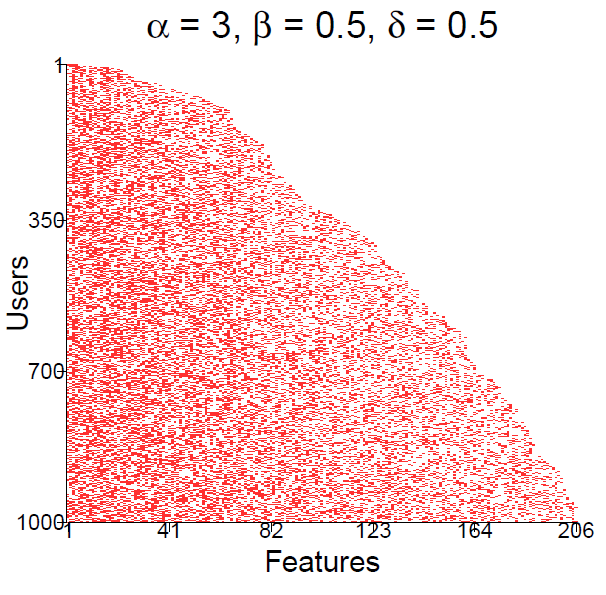
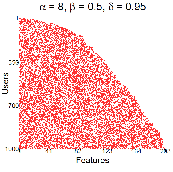
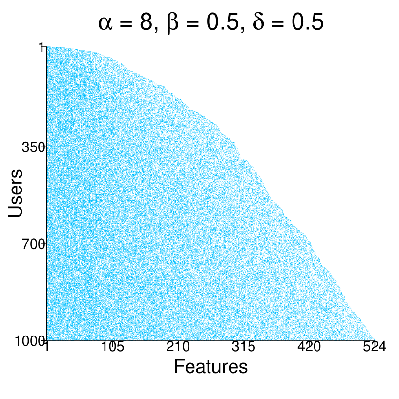
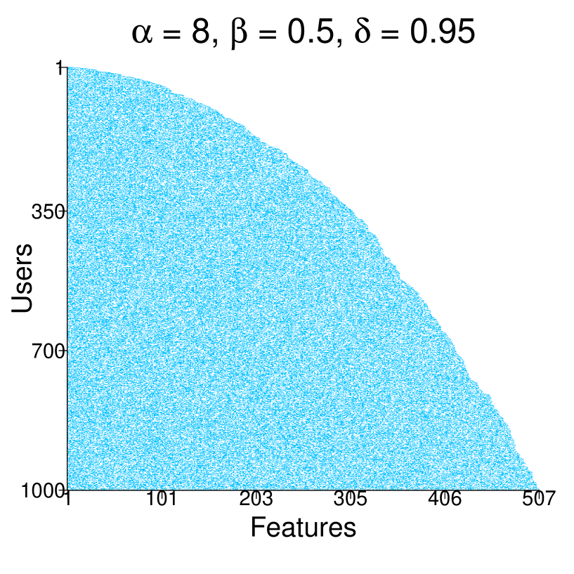
Figure 4: Examples of features matrices for $n=1000$, $\beta=0.5$, different values of $\alpha:3$ (top), $8$ (bottom) and different values of $\delta:0.1$ (left), $0.5$ (middle), $0.95$ (right). Colored points denote $1$ and white points denote $0$.

	$\delta\,=\,0.1$	$\delta\,=\,0.5$	$\delta\,=\,0.95$
$\alpha=3$	0.1005	0.1119	0.0099
$\alpha=8$	0.1010	0.1129	0.0097

Table 2: Measure of the “uniformity” of the feature matrix defined as the difference (averaged over $100$ realizations) between the mean number of nodes per feature for the first and the second half of the features’ set. Considered parameters: $\alpha=3,\,8$, $\beta=0.5$ and $\delta=0.1,\,0.5,\,0.95$.

6.2 Simulations of the unipartite network and procedure in order to recover $K$ and $\vartheta$

We performed the simulations of the unipartite network as follows. Once a feature matrix $F$ is generated, links are created according to the two phases of the link construction described in Section 3, taking $\Phi$ as in (4.1). We simulated the network for $n=1\,000$ nodes on a sample of $100$ realizations.

In the first set of experiments, we fixed a number $\ell$ of links and we determined the value of $\vartheta$, for different values of $K$, by solving (numerically) the equation

$$\sum_{i=2}^{n}\sum_{j=1}^{i-1}\left(1+e^{K(\vartheta-\sum_{k=1}^{L_{i}}F_{i,k}F_{j,k})}\right)^{-1}=\ell\,,$$ (6.1)

in order to have the expected number of (undirected) links due to the first phase of the unipartite network construction equal to the given number $\ell$. Hence, we studied the network structure as a function of the parameters $K$ and $p$ (related to the link formation). In particular, we recall that $p$ increases the triadic closure phenomenon. We also considered different values of $\delta$, that regulates the preferential attachment in the transmission of the features and so influences the shape of the feature matrix $F$. In the Appendix we report the results.

With the second set of experiments, we studied the accuracy of the procedure (5.5) used in order to recover $K$ and $\vartheta$. Hence, we fixed $\alpha=10$, $\beta=0.5$, $\delta=0.1$, $K=1$, $\vartheta=10$, and $p=0$ (so that $A^{\prime}=A$) and we generated a sample of $R=100$ realizations of the network. We then applied the procedure (5.5) to each realization $r$ (with $s^{*}=10$) in order to get the corresponding values ${\widehat{K}}_{r}$ and ${\widehat{\vartheta}}_{r}$. We found:

$$\begin{split}&\frac{1}{R}\sum_{r=1}^{R}{\widehat{K}}_{r}=1.000462,\qquad MSE_{K}=\frac{1}{R}\sum_{r=1}^{R}({\widehat{K}}_{r}-K)^{2}=0.00415,\\ &\frac{1}{R}\sum_{r=1}^{R}{\widehat{\vartheta}}_{r}=9.998843,\qquad MSE_{\vartheta}=\frac{1}{R}\sum_{r=1}^{R}({\widehat{\vartheta}}_{r}-\vartheta)^{2}=0.00010.\end{split}$$

7 Application to a co-authorship network

We downloaded bibliographic information of papers and preprints found in the IEEE Xplore database [62]. In this dataset a link is taken as the co-authorship of a paper between two or more authors and the contexts of the papers are given by $2$-grams (pairs of sequential words in the title or abstract). We selected the papers using search terms related to the specific research area of autonomous cars (also called connected cars).

7.1 Description of the dataset

We downloaded (on Aug. 7, 2014) all papers in the IEEE preprint and paper archive using $17$ specific search terms: ‘Lane Departure Warning’, ‘Lane Keeping Assist’, ‘Blindspot Detection’, ‘Rear Collision Warning’, ‘Front Distance Warning’, ‘Autonomous Emergency Braking’, ‘Pedestrian Detection’, ‘Traffic Jam Assist’, ‘Adaptive Cruise Control’, ‘Automatic Lane Change’, ‘Traffic Sign Recognition’, ‘Semi-Autonomous Parking’, ‘Remote Parking’, ‘Driver Distraction Monitor’, ‘V2V or V2I or V2X’, ‘Co-Operative Driving’, ‘Telematics & Vehicles’, and ‘Night vision’. The IEEE archive returned all the papers in their database that contain these terms in the title or abstract, and we downloaded the bibliographic records for all returned papers including the authors, title, abstract, and the date on which the paper was added to the database. This download yielded $6\,129$ distinct papers with a complete bibliographic record and at least two authors. While these search terms can not be expected to yield all papers related to automated car research, we expect to have found a relatively broad panel of related papers.

7.2 Analysis of the feature-structure

The feature matrix was built by extracting all $2$-grams (pairs of words) appearing in either the title or abstract of a paper. The text was converted to lowercase, removing all punctuation (with the exception of the ‘/’ and ‘.’ characters) and multi-spaces, and split into individual sentences. The $2$-grams occurring in any sentence in the title or abstract were labeled as features of the paper. In order to remove spurious $2$-grams (e.g. ‘this paper’ often occurs in the abstract, but it is not relevant to connected cars), we exclude any $2$-grams containing any of the words: ‘the’, ‘a’, ‘of’, ‘and’, ‘to’, ‘is’, ‘for’, ‘in’, ‘an’, ‘with’, ‘by’, ‘from’, ‘on’, ‘or’, ‘that’, ‘at’, ‘be’, ‘which’, ‘are’, ‘as’, ‘one’, ‘may’, ‘it’, ‘and/or’, ‘if’, ‘via’, ‘can’, ‘when’, ‘we’, ‘his’, ‘her’, ‘their’, ‘this’, ‘our’, ‘into’, ‘has’, ‘have’, ‘only’, ‘also’, ‘do’, ‘does’, ‘presents’, ‘paper’, ‘doesn’t’, and ‘not’. This approach gave $155\,897$ distinct $2$-grams (features) for a total of $6\,129$ papers (nodes). We ordered the papers chronologically based on their entry date into the IEEE database (which we expect to be a good proxy for their publication date). The $2$-grams were ordered in terms of their first appearance in a paper (as described in Section 2).

Having extracted the set of the $2$-grams contained in each paper, we constructed the feature-matrix $F$, with $F_{ik}=1$ if paper $i$ contains the $2$-gram $k$ and $F_{ik}=0$ otherwise. The resulting matrix $F$ is shown in Fig. 5(a), with non-zero values of $F$ indicated by colored points. We also simulated the feature-matrix for a smaller network of $1000$ nodes taking the parameters equal to the corresponding estimated values (see Fig. 5(b)). The number of features obtained in the simulation is $28\,664$, which is consistent with the observed matrix.

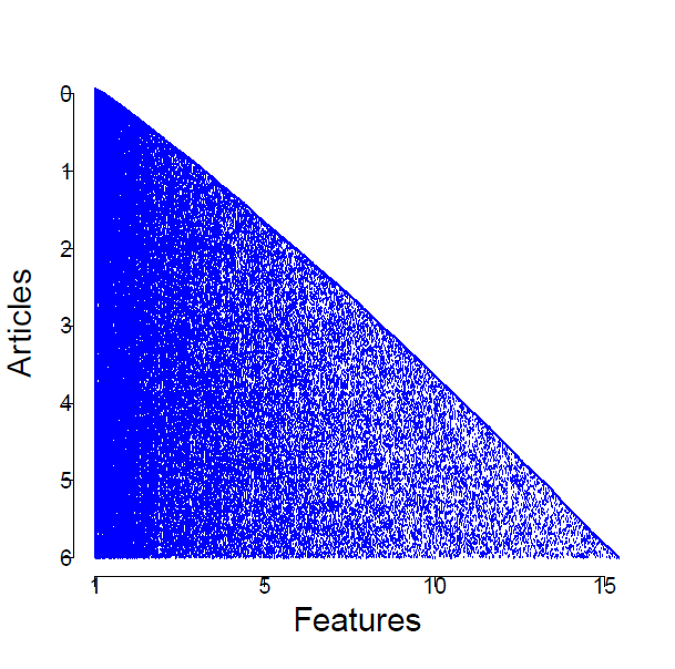
(a)

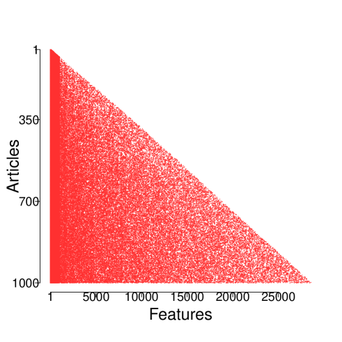
(b)

Figure 5: (a) Feature-matrix associated to the dataset. Dimensions: $6\,129$ nodes (papers) $\times$ $155\,897$ features ($2$-grams). Colored points denote $1$ and white points denote $0$. (b) Feature matrix for $1000$ nodes, obtained by simulation of the model with $\alpha=\widehat{\alpha}=32.28$, $\beta=\widehat{\beta}=0.98$, and $\delta=\widehat{\delta}=0.0057$. Colored points denote $1$ and white points denote $0$. The total number of features is $28\,664$, which is consistent with the observed matrix.

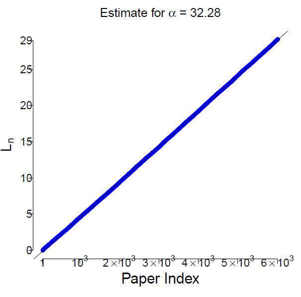
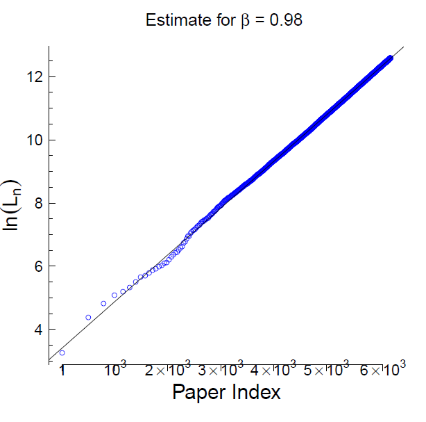
Figure 6: Estimated values of the model parameters $\alpha$ and $\beta$.

The growth of the cumulative count $L_{n}$ of the distinct $2$-grams (the number of distinct $2$-grams seen until the $n^{th}$ paper included, as described in Section 2) is shown in Fig. 6(b) in a log-log scale and it shows a clear power-law behavior, with estimated parameter $\widehat{\beta}=0.98$ (that corresponds to the estimated value of the model parameter $\beta$). Regarding the model parameter $\alpha$, we get the estimated value $\widehat{\alpha}=32.28$ and in Fig. 6(a) we show the corresponding fit plotting the cumulative count $L_{n}$ of the $2$-grams as a function of $n^{\widehat{\beta}}$. Finally, the estimated value for the parameter $\delta$ is $\widehat{\delta}=0.0057$. As we can see, this last value is very small and so we can conclude that the preferential attachment rule in the transmission of the features plays an important role.

7.3 Analysis of the unipartite network

Our dataset includes $6\,129$ papers for a total of $13\,581$ distinct author names. The considered unipartite network is constructed taking the papers as nodes and drawing a link between two nodes if they share at least one author. We harmonized the author names across different papers by ensuring that the authors’ last names are always found in the same position and removed any stray punctuation in the names. No further disambiguation was performed, meaning that authors who may use their full names in some papers but only their initials in other papers will be treated as distinct. For example, the names “J. J. Anaya” and “Jose Javier Anaya” are treated as distinct authors in our dataset, while it is possible that these distinct names refer to the same person. A full disambiguation of author names is computationally difficult [39], and beyond the scope of this paper. This approach gave a unipartite network with $19\,065$ links that involve $4\,712$ nodes in the network. This means that there is a set of $1\,417$ isolated nodes, where a paper has two or more authors that are not listed on any other paper in the dataset. However, we decided to also consider these nodes in our analysis since we included them in the features matrix as nodes that can potentially link to other nodes.

The distribution of the $2$-grams (the features) in common between two papers (the nodes) given the presence or the absence of at least one shared author (i.e. given the presence or the absence of a link between them) is plotted in Figure 7(a). The curve with (red) triangles is the distribution of the number of $2$-grams shared by two papers given they have at least one co-author. More precisely, for each value on the $x$-axis, we have on the $y$-axis the fraction

$$\frac{\hbox{num. of pairs of papers with }x\,\hbox{2-grams in common and at least 1 shared author}}{\hbox{num. of pairs of papers with at least 1 shared author}}.$$ (7.1)

The curve with (green) stars represents the distribution of the number of $2$-grams shared by two papers given they have no authors in common, i.e. it is given by the same formula as (7.1) but with pairs of papers without shared authors. As we can see, there is a higher probability of common $2$-grams when there are shared authors.

The fraction of pairs of papers with $x$ $2$-grams in common that have at least one shared author is plotted in Figure 7(b) by the curve with (red) triangles. More precisely, for each value on the $x$-axis, we have on the $y$-axis the fraction

$$\frac{\hbox{num. of pairs of papers with }x\,\hbox{2-grams in common and at least 1 shared author}}{\hbox{num. of pairs of papers with }x\,\hbox{2-grams in common}}.$$ (7.2)

As we can see, the plotted fraction increases with the number of features in common.

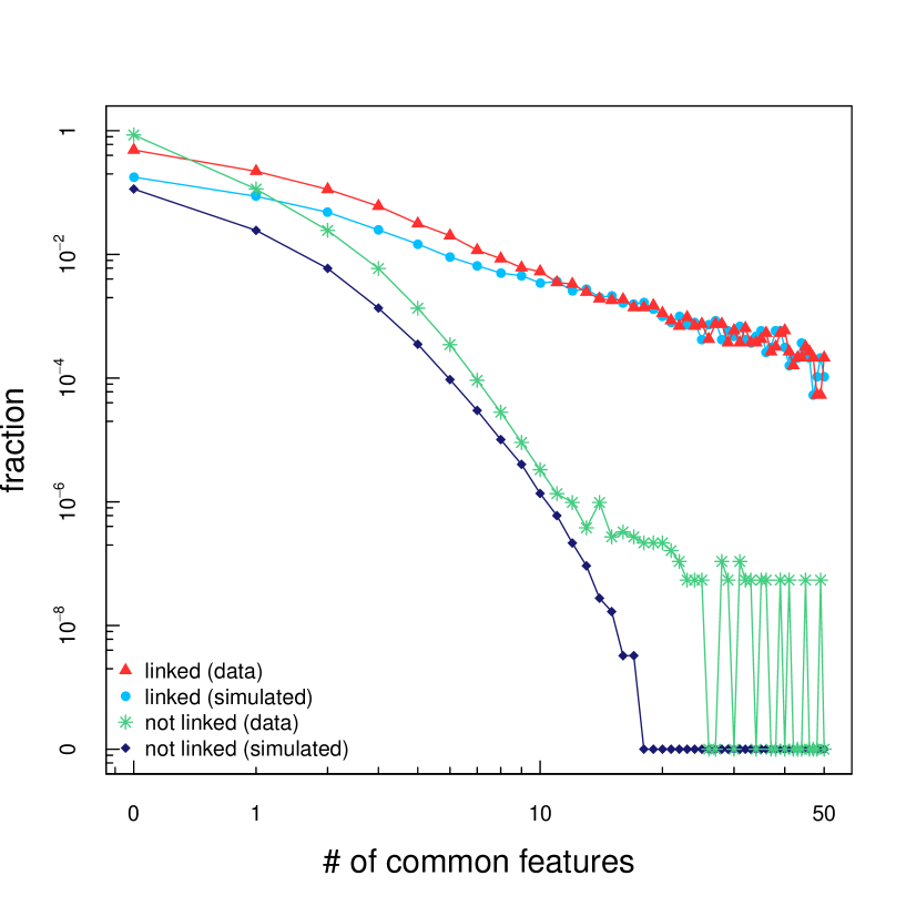
(a)

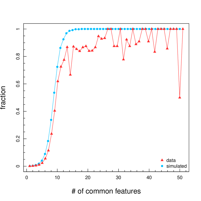
(b)

Figure 7: (a) Distribution of the $2$-grams (features) in common between two papers (nodes) given the presence (red triangles for the real data and light blue circles for the simulated ones) or the absence (green stars for the real data and dark blue squares for the simulated ones) of at least one co-author. (b) Fraction of pairs of papers with $x$ $2$-grams in common that have at least one co-author, for the real data case (red triangles) and for the simulated one (light blue circles).

The network is composed of $586$ connected components with at least one edge and $1\,417$ isolated nodes (a total of $2\,003$ components). The largest connected component has $2\,776$ nodes and $16\,108$ links, so about the $45\%$ of the nodes can reach each other in the largest connected component and it includes about the $84\%$ of the links. The diameter (i.e. the maximum distance between nodes) of the largest connected component is $23$. The other $585$ connected components (disconnected from the largest component but still having at least one edge) globally contain $1\,936$ nodes, and over $90\%$ of the components (containing over $75\%$ of the nodes outside of the largest connected component) contain $7$ or fewer nodes. Hence the percentage of reachable pairs (denoted by $RP$ in the remainder of the paper) of nodes in the network is about $20.51\%$.

We decided to first use the model with $p=0$ in order to have a benchmark and then try to guess a good value for $p$. Taking $p=0$, we set $A^{\prime}=A$ (i.e. links are only formed by means of the first phase) and we applied the procedure (5.5) to the observed feature-matrix $F$ with $s^{*}=10$ (the corresponding value for $f^{*}$ is $0.725$) and $\ell=19\,065$ in order to detect $K$ and $\vartheta$: we found $\widehat{K}=0.8228$ and $\widehat{\vartheta}=8.8201$. We then generate a sample of $100$ realizations of the network by simulating the model starting from the observed matrix $F$ and with $p=0$, $K={\widehat{K}}=0.8228$, and $\vartheta={\widehat{\vartheta}}=8.8201$. We obtained a network structure very different from the observed one (for instance, $RP=99\%$). This can be obviously explained by the fact that we set $p=0$ (benchmark case), while a value of $p$ strictly greater than $0$ is guessable. Indeed, an author with $m\geq 3$ papers automatically guarantees a minimum of $m\choose 3$ triangles. Setting $p=0.7$ and generating a sample of $100$ realizations of the network by simulating the model starting from the observed matrix $F$ , we succeeded to capture a value for $RP$ very near to the observed one, i.e. $RP=19.61\%$ (this value is an average over the $100$ realizations). Moreover, we obtained that the largest connected component contains on average $2\,689.16$ nodes, again a value near to the observed one. Finally, Figure 7(a) contains the distribution of the features in common between two nodes given the presence (light blue circles) or the absence (dark blue squares) of a link between them and Figure 7(b) depicts the fraction of pairs of nodes with $x$ features in common that are linked. Although the curves related to real data are obviously more irregular, the curves generated by simulations properly fit to the observed ones.

8 Conclusions and discussion on some variants of the model

In this paper, we presented a new network model, where each node is characterized by a number of features and the probability of a link between two nodes depends on the number of features and neighbors they share, so that it includes two of the most observed phenomena in complex systems: assortativity, i.e. the prevalence of network-links between nodes that are similar to each other in some sense, and triadic closure, meant as the high probability of having a link between a pair of nodes due to common neighbors. The bipartite network of nodes and features grows according to a stochastic dynamics that depends on three parameters respectively regulating the preferential attachment in the transmission of the features to the nodes, the number of new features per node, and the power-law behavior of the total number of observed features. We provide theoretical results and statistical tools for the estimation of the model parameters involved in the feature-structure dynamics. From the observation of the feature-matrix, we completely determine the parameters, $\alpha,\beta,\delta$, that regulate its evolution. We provide a procedure for recovering the two parameters, $K,\,\vartheta$, of the function $\Phi$, which relates the link probability between two nodes to their similarity in terms of common features, and the parameter $p$ which tunes triadic closure. However, as discussed in Section 5, for this last point, we need to know which are the links formed by assortativity and those formed by triadic closure, but often they are not easily distinguishable. Therefore we aim in the future to evaluate more sophisticated estimation techniques for this issue. Nevertheless, as shown in Section 7, we can still exploit the proposed procedure in order to guess a good combination of these parameters.

The originality and the merit of our model mainly lie in the double temporal dynamics (one for the feature-structure and one for the network of nodes), but also in the attention given to both assortativity and triadic closure mechanisms. We underline that, differently from other models in the literature, we do not require to specify a priori the values of some hyperparameters, such as the total number of possible features (avoiding some selection problems discussed in [37]). In the future, we aim at improving our model in order to make it suitable for other kind of networks, e.g. real social networks (such as friendship networks). In particular, the following variations are possible:

• Normalizing the number of common features: We can vary the model by replacing the factor $F_{i,k}F_{j,k}$ in formula (3.3) with

  $$\frac{F_{i,k}F_{j,k}}{\sum_{j^{\prime}=1}^{i-1}F_{j^{\prime},k}},\,\forall(i,j)\mbox{ with }1\leq j\leq i-1,$$

  so that the contribution of a common feature $k$ is smaller when the number of nodes with $k$ as a feature is larger.

• Weighted bipartite matrices: We can modify the model by replacing in the inclusion-probability and in the link-probability the binary random number $F_{i,k}$ by a random weight $W_{i,k}$ of the form $W_{i,k}=F_{i,k}Y_{i,k}/(\sum_{k=1}^{L_{i}}F_{i,k}Y_{i,k})$, where $Y_{i,k}$ are i.i.d. strictly positive random variables. (By convention, we set $0/0=0$.) Hence, we have

  $$W_{i,k}\in[0,1]\quad\mbox{and}\quad\sum_{k=1}^{L_{i}}W_{i,k}=1$$

  so that $W_{i,k}$ represents the weight percentage given to feature $k$ by node $i$. Therefore, the preferential attachment in the inclusion-probability becomes a “weighted preferential attachment”, in the sense that it depends on the total weight given to feature $k$ by the previous nodes, and the link-probability depends on the weights associated to the common features.

• Changeable links: For some real situations, we need to consider also the case in which the links among nodes can change along time. For instance, we can combine a link-formation model and a link-dissolution model as in [36]. See also [26] for node exit.

• Exit of some features and social influence of links on features: We can modify the evolution of the feature-structure by accounting for the fact that at each time step $j$ (after the arrival of the node $j$) some features can become “obsolete” and so for such a feature $k$ we will have $F_{i,k}=0$ for all $i\geq j+1$. Moreover, a node could change some features under the influence of its “friends” (i.e. neighbors) [26]. Hence, we can introduce a sequence $(F^{(i)})_{i}$ of bipartite matrices such that each $F^{(i)}$ provides the features before the arrival of node $i+1$, so that in the inclusion-probabilities and in the link-probabilities for node $i+1$, the matrix $F$ is replaced by $F^{(i)}$.

• Different dynamics for triadic closure: We can change the second phase of our model by means of different policies for the selection of additional neighbors of a node $i$ among the neighbors of $i$’s neighbors. Indeed, in this paper we consider a binomial model according to which each common neighbor of a pair $(i,j)$ of not-linked nodes gives, independently of the others, a probability $p$ of inducing a link between $i$ and $j$. A possible alternative is that, with probability $p$, an additional link for a certain node is formed by the selection (uniformly at random) of a node among the neighbors of its neighbors (e.g. [10]).
  

Acknowledgments and Financial Support

Authors acknowledge support from CNR PNR Project “CRISIS Lab”.

Appendix A Appendix

A.1 Proof of the asymptotic behavior of $L_{n}$

Theorem A.1.

Consider our model, the following statements hold true:

• ${L_{n}}/{\ln(n)}\stackrel{{\scriptstyle a.s.}}{{\longrightarrow}}\alpha$ for $\beta=0$;

• ${L_{n}}/{n^{\beta}}\stackrel{{\scriptstyle a.s.}}{{\longrightarrow}}{\alpha}/\beta$ for $\beta\in(0,1]$.

Proof.

Set $\lambda_{1}=\alpha$ and recall that the random variables $N_{i}$ are independent and each $N_{i}$ has distribution Poi$(\lambda_{i})$.

The assertion b) is trivial for $\beta=1$ since, in this case, $L_{n}$ is the sum of $n$ independent random variables with distribution $\hbox{Poi}(\alpha)$ and so, by the classical strong law of large numbers, $L_{n}/n\stackrel{{\scriptstyle a.s.}}{{\longrightarrow}}\alpha$.

Now, let us prove assertions a) and b) for $\beta\in[0,1)$. Define

$$\lambda(\beta)=\alpha\,\text{ if }\,\beta=0\quad\text{and}\quad\lambda(\beta)=\frac{\alpha}{\beta}\,\,\text{ if }\,\beta\in(0,1),$$

$$a_{n}(\beta)=\log{n}\,\text{ if }\,\beta=0\quad\text{and}\quad a_{n}(\beta)=n^{\beta}\,\text{ if }\,\beta\in(0,1).$$

We need to prove that $L_{n}/a_{n}(\beta)\stackrel{{\scriptstyle a.s.}}{{\longrightarrow}}\lambda(\beta)$. First, we observe that

$$\frac{\sum_{i=1}^{n}\lambda_{i}}{a_{n}(\beta)}=\alpha\frac{\sum_{i=1}^{n}i^{\beta-1}}{a_{n}(\beta)}\longrightarrow\lambda(\beta),$$

Next, let us define

$$T_{0}=0\quad\text{and}\quad T_{n}=\sum_{i=1}^{n}\frac{N_{i}-E[N_{i}]}{a_{i}(\beta)}=\sum_{i=1}^{n}\frac{N_{i}-\lambda_{i}}{a_{i}(\beta)}.$$

Then $(T_{n})$ is a martingale with

$$E[T_{n}^{2}]=\sum_{i=1}^{n}\frac{E\bigl{[}(N_{i}-\lambda_{i})^{2}\bigr{]}}{a_{i}(\beta)^{2}}=\sum_{i=1}^{n}\frac{\lambda_{i}}{a_{i}(\beta)^{2}}$$

and so $\sup_{n}E[T_{n}^{2}]=\sum_{i=1}^{+\infty}\frac{\lambda_{i}}{a_{i}(\beta)^{2}}<+\infty$. Thus, $(T_{n})$ converges a.s. and the Kronecker’s lemma implies

$$\frac{1}{a_{n}(\beta)}\sum_{i=1}^{n}a_{i}(\beta)\frac{(N_{i}-\lambda_{i})}{a_{i}(\beta)}\stackrel{{\scriptstyle a.s.}}{{\longrightarrow}}0,$$

that is

$$\frac{\sum_{i=1}^{n}N_{i}}{a_{n}(\beta)}-\frac{\sum_{i=1}^{n}\lambda_{i}}{a_{n}(\beta)}\stackrel{{\scriptstyle a.s.}}{{\longrightarrow}}0.$$

Therefore, we can conclude that

$$\lim_{n}\frac{L_{n}}{a_{n}(\beta)}=\lim_{n}\frac{\sum_{i=1}^{n}N_{i}}{a_{n}(\beta)}=\lim_{n}\frac{\sum_{i=1}^{n}\lambda_{i}}{a_{n}(\beta)}=\lambda(\beta)\quad\text{a.s.}$$

∎

Remark A.2.

The above Theorem implies that $\ln(L_{n})/\ln(n)$ is a strongly consistent estimator of $\beta$. Indeed, if $\beta=0$ then $L_{n}\stackrel{{\scriptstyle a.s.}}{{\sim}}\alpha\ln(n)$ as $n\to+\infty$; hence $\ln(L_{n})\stackrel{{\scriptstyle a.s.}}{{\sim}}\ln(\alpha)+\ln(\ln(n))$, therefore $\ln(L_{n})/\ln(n)\stackrel{{\scriptstyle a.s.}}{{\sim}}\ln(\alpha)/\ln(n)+\ln(\ln(n))/\ln(n)\stackrel{{\scriptstyle a.s.}}{{\to}}0=\beta$. Furthermore, if $\beta>0$, then we have $L_{n}\stackrel{{\scriptstyle a.s.}}{{\sim}}(\alpha/\beta)n^{\beta}$ as $n\to+\infty$ so $\ln(L_{n})\stackrel{{\scriptstyle a.s.}}{{\sim}}\ln(\alpha/\beta)+\beta\ln(n)$, hence $\ln(L_{n})/\ln(n)\stackrel{{\scriptstyle a.s.}}{{\sim}}\ln(\alpha/\beta)/\ln(n)+\beta\stackrel{{\scriptstyle a.s.}}{{\to}}\beta$.

A.2 Simulations of the unipartite network: some analysis on its structure

We generated feature matrices with $n=1\,000$ nodes taking fixed values for $\alpha$ and $\beta$, i.e. $\alpha=10$ and $\beta=0.5$, and different values for $\delta$ ($\delta\in[0.1,\,0.5]$). Starting from these feature matrices, we considered the structure of the unipartite network for three different values of $K$ ($K=1,\,4,\,10$) and three different values of $p$ ($p=0,\,0.1,\,0.5$).

We considered the following quantities:

• the clustering coefficient defined as:

  $$C=\frac{\hbox{Number of closed triplets}}{\hbox{Number of connected triplets of nodes}},$$ (A.1)

  where a connected triplet is a set of three nodes that are connected by two or three undirected links (open and closed triplet, respectively). See Table 3.

• the fraction of pairs of nodes at distance at most $20$, i.e. the fraction of pairs of nodes that are reachable from each other within at most $20$ steps (see Table 4):

  $$RP_{20}=\frac{\hbox{Number of couples of nodes at distance at most $20$}}{\hbox{Number of couples of nodes}}.$$ (A.2)

  We recorded also the observed maximum value $h^{*}$ of the distance between the nodes.

• the degree distribution, in the sense of the Complementary Cumulative Distribution Function (CCDF) of the number of neighbors of each node (see Figure 8).

The clustering coefficient $C$ strongly increases with $p$ (as expected). For $p=0$ the percentage of closed triplets increases with $\delta$, but remains smaller or equal than $13\%$ of total triplets for all considered values of $\delta$ and $K$. For values of $p$ greater than zero, the percentage of closed triplets increases with $\delta$ in a range of $13\%-30\%$ for $p=0.1$ and in a range of $39\%-62\%$ for $p=0.5$. The effect of $K$ and $\delta$ seems to be marginal on the clustering coefficient.

		$\delta\,=$	0.1	0.15	0.2	0.25	0.3	0.35	0.4	0.45	0.5
	$p\,=\,0$		0.04	0.05	0.07	0.08	0.08	0.10	0.13	0.13	0.10
$K=1$	$p\,=\,0.1$		0.13	0.17	0.20	0.23	0.23	0.24	0.26	0.27	0.30
	$p\,=\,0.5$		0.39	0.45	0.45	0.49	0.49	0.47	0.49	0.53	0.62
	$p\,=\,0$		0.06	0.06	0.08	0.09	0.08	0.11	0.13	0.13	0.11
$K=4$	$p\,=\,0.1$		0.15	0.18	0.21	0.24	0.23	0.25	0.26	0.28	0.30
	$p\,=\,0.5$		0.42	0.47	0.46	0.49	0.49	0.48	0.50	0.53	0.62
	$p\,=\,0$		0.06	0.06	0.08	0.09	0.08	0.11	0.13	0.14	0.11
$K=10$	$p\,=\,0.1$		0.15	0.18	0.21	0.24	0.23	0.25	0.26	0.28	0.30
	$p\,=\,0.5$		0.42	0.47	0.46	0.49	0.49	0.48	0.49	0.53	0.62

Table 3: Clustering coefficient (averaged over $100$ realizations) for $\alpha=10$, $\beta=0.5$, $\ell=4000$, and different values of $\delta$, $K$, and $p$.

Looking at the values obtained for the fraction of pairs of nodes at distance at most $20$, for the two different values $\delta=0.1$ and $\delta=0.5$, we can notice a clear difference in the behavior (independently of $K$ and $p$): indeed, the fraction of reachable pairs for $\delta=0.1$ (when $K$ and $p$ are fixed) is highly greater than the corresponding fraction for $\delta=0.5$. Moreover, the fraction of reachable pairs decreases when $K$ increases (and the other parameters are fixed) and slightly changes when only $p$ varies. The complementary fraction corresponds to the pairs of nodes at distance greater than $20$ or not reachable from each other.
The observed maximum distance $h^{*}$ (among pairs of nodes at distance at most $20$) varies in range of $2-5$ and decreases when $\delta$ ($p$ and $K$, respectively) increases and the other parameters are fixed.

		$K=1$		$K=4$		$K=10$
	$\delta=$	0.1	0.5	0.1	0.5	0.1	0.5
$p=0$		0.439 ($5$)	0.128 ($4$)	0.350 ($4$)	0.118 ($4$)	0.349 ($4$)	0.117 ($4$)
$p=0.1$		0.438 ($4$)	0.128 ($3$)	0.352 ($3$)	0.118 ($3$)	0.350 ($3$)	0.117 ($3$)
$p=0.5$		0.437 ($3$)	0.128 ($2$)	0.351 ($2$)	0.118 ($2$)	0.349 ($2$)	0.117 ($2$)

Table 4: Fraction of pairs of nodes at distance at most $20$ (averaged over $100$ realizations) for $\alpha=10$, $\beta=0.5$, $\ell=4000$, and different values of $\delta$, $K$, and $p$. For each set of parameters, the corresponding observed maximum distance $h^{*}$ is reported in brackets.

Finally, the effect of $p$ on the total number of links is clear: when $p=0$ the number of links is approximately equal to the chosen $\ell$ (i.e. $\ell=4000$), since in this case we have only the first phase of the unipartite network construction: links are related only to the features. The larger $p$ the more triangles are closed and so the more links we have. Table 5 reports the total number of links for all combinations of the parameters. Regarding the degree distribution, Figure 8 shows the CCDF of the number of neighbors of a node. Parameter $p$ also influences the shape of the degree distribution, together with $\delta$ and $K$.

		$K=1$		$K=4$		$K=10$
	$\delta\,=$	0.1	0.5	0.1	0.5	0.1	0.5
$p\,=\,0$		4 003.47	3 998.15	4 002.17	3 999.59	3 997.13	3 999.52
$p\,=\,0.1$		17 853.46	19 862.54	19 107.53	19 523.42	19 112.46	19 484.86
$p\,=\,0.5$		93 093.05	43 538.68	81 343.97	41 382.62	81 039.49	41 156.34

Table 5: Total number of links in the unipartite network (averaged over $100$ realizations) for $\alpha=10$, $\beta=0.5$, $\ell=4000$, and $\delta$, $K$, and $p$ varying. Note that for $p=0$ the number is around the chosen $\ell=4000$.

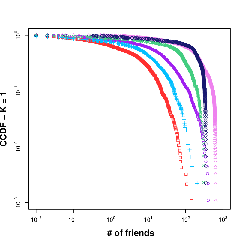
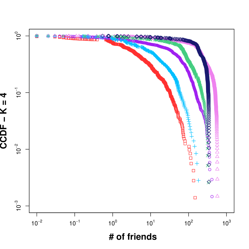
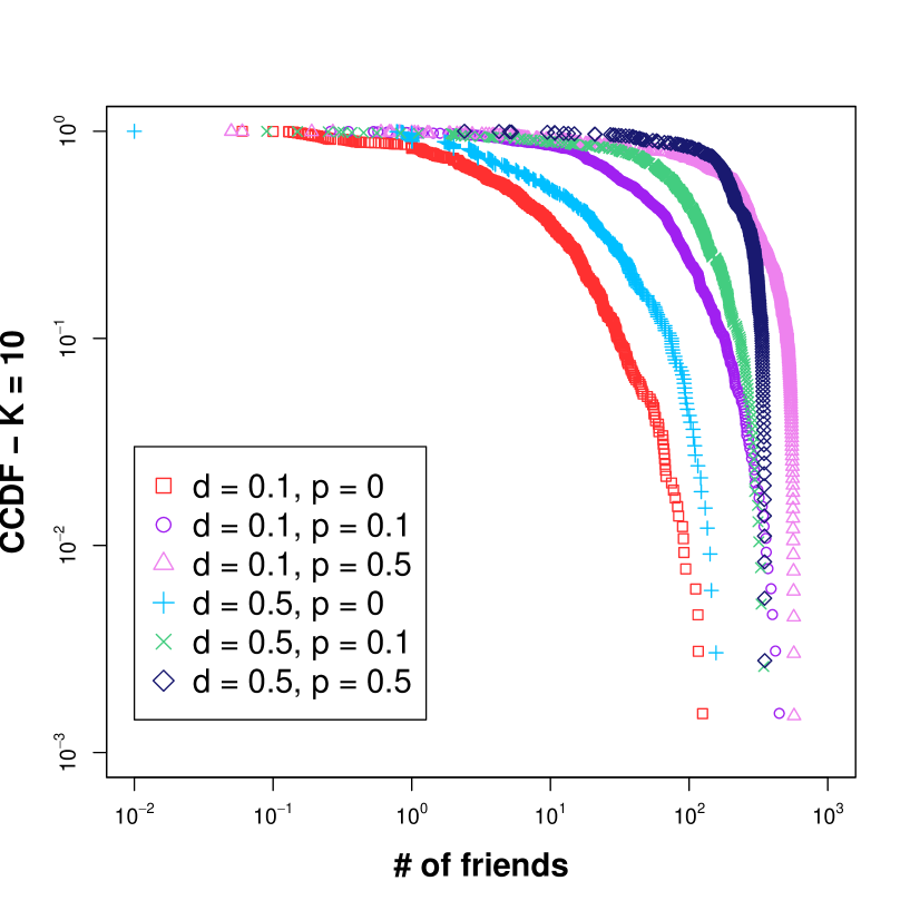
Figure 8: CCDF of the number of neighbors (averaged over $100$ realizations) for $\alpha=10$, $\beta=0.5$, $\ell=4000$, and different values of $K$ (corresponding to different boxes) and different values of $\delta$ and $p$ (corresponding to different symbols and colors).

References

- [1] Airoldi E., Blei D., Fienberg S. and Xing E. (2008) Mixed membership stochastic block-models. Journal of Machine Learning Research, 9, 1981-2014.
- [2] Bagler G. and Sinha S. (2007) Assortative mixing in protein contact networks and protein folding kinetics. Bioinformatics 23 (14), 1760-1767.
- [3] Barabási A. L. and Albert R. (2002) Statistical mechanics of complex networks. Reviews of modern physics 74, 47-97.
- [4] Barabási A. L. and Albert R. (1999) Emergence of scaling in random networks. Science 286, 509-512.
- [5] Barabási A. L., Jeong H., Neda Z., Ravasz E., Schubert A. and Vicsek T. (2002) Evolution of the social network of scientific collaborations. Physica A, 311, 590-614.
- [6] Barrat A., Barthlemy M. and Vespignani A. (2008) Dynamical processes on complex networks. Cambridge University Press.
- [7] Berti P., Crimaldi I., Pratelli L. and Rigo P. (2015) Central limit theorems for an Indian buffet model with random weights. The Annals of Applied Probability 25(2), 523-547.
- [8] Bessi A., Caldarelli G., Del Vicario M., Scala A. and Quattrociocchi W. (2014) Social determinants of content selection in the age of (mis)information. Proceedings of SOCINFO 2014; abs/1409.2651.
- [9] Blau P. M. and Schwartz J. E. (1984) Crosscutting social circles: testing a macrostructural theory of intergroup relations, Academic Press, Orlando (FL).
- [10] Bianconi G., Darst R. K., Iacovacci J. and Fortunato S. (2014) Triadic closure as a basic generating mechanism of communities in complex networks. Physical Review E, 90(4), 042806.
- [11] Block P. and Grund T. (2014) Multidimensional homophily in friendship networks. Network Science, 2(02), 189-212.
- [12] Boldi P., Crimaldi I. and Monti C. A network model characterized by a latent attribute structure with competition. Under review. Currently available on arXiv 1407.7729.
- [13] Bramoullé Y., Currarini S., Jackson M. O., Pin P. and Rogers B. W. (2012) Homophily and long-run integration in social networks. Journal of Economic Theory, 147(5), 1754-1786.
- [14] Brown J., Broderick A. J. and Lee N. (2007) Word of mouth communication within online communities: Conceptualizing the online social network. Journal of interactive marketing, 21(3), 2-20.
- [15] Caldarelli G. (2007) Scale-Free Networks: complex webs in nature and technology. OUP Catalogue.
- [16] Currarini S., Jackson M. O. and Pin P. (2009) An economic model of friendship: Homophily, minorities, and segregation. Econometrica, 77(4), 1003-1045.
- [17] Currarini S. and Vega-Redondo F. (2013) A simple model of homophily in social networks. University Ca’ Foscari of Venice, Dept. of Economics Research Paper Series, (24).
- [18] Easly D. and Kleinberg J. (2010) Networks, Crowds and Markets: Reasoning about a highly connected world. Cambridge Univ. Press.
- [19] Feld S. L. (1982) Social structural determinants of similarity among associates. American Sociological Review, 47(6), 797-801.
- [20] Goldenberg A. and Zhen E. (2009) A survey of statistical network models. Foundations and trends in Machine Learning, 2, 129-233.
- [21] Golub B. and Jackson M. O. (2009) How homophily affects the speed of learning and best response dynamics. Quart. J. Econ., forthcoming.
- [22] Goodreau S. M., Kitts J. A. and Morris M. (2009) Birds of a feather, or friend of a friend? Using Exponential Random Graph Models to investigate Adolescent Social Networks. Demography, 46(1), 103-125.
- [23] Handcock M. S., Raftery A. E. and Tantrum J. M. (2007) Model-based clustering for social networks. Journal of the Royal Statistical Society, series A, 170, 301-354.
- [24] Hanneke S., Fu W. and Xing E. P. (2010) Discrete temporal models of social networks. Electronic Journal of Statistics, 4, 585-605
- [25] Hoff P. D., Raftery A. E. and Handcock M. S. (2002) Latent space approaches to social network analysis. J. American Statistical Ass., 97, 1090-1098.
- [26] Huisman M. and Snijders T. A. B. (2003) Statistical Analysis of longitudinal network data with changing composition. Sociological methods and research, 32(2), 253-287.
- [27] Hunter D. R., Krivitsky P. N. and Schweinberger M. (2012) Computational statistical methods for social network models. J. comput. Graph Stat., 21(4), 856-882.
- [28] Ispolatov I., Krapivsky P. L. and Yuryev A. (2005). Duplication-divergence model of protein interaction network. Phys. Rev. E., 71(6).
- [29] Jackson M. O. (2014) Networks in the understanding of economic behaviors, The Journal of Economic Perspectives (2014), 3-22.
- [30] Jackson M. O. (2008). Social and Economic Networks. Princeton University Press.
- [31] Jackson M. O. and Rogers B. W. (2007) Meeting strangers and friends of friends: How random are social networks? The American economic review, 97(3), 890-915.
- [32] Kandel D. A. (1978) Homophily, selection, and socialization in adolescent friendships, American Journal of Sociology, 84(2), 427-436.
- [33] Kolaczyk E. D. (2009) Statistical analysis of network data: methods and models. Springer.
- [34] Kossinets G. and Watts, D. J. (2009) Origins of homophily in an evolving social network. American Journal of Sociology, 115(2), 405-450.
- [35] Kossinets G. and Watts D. J. (2006) Empirical analysis of an evolving social network. Science 311.
- [36] Krivitsky P. N., Handcock M. S. (2014) A separable model for dynamic networks. Journal of the Royal Statistical Society, series B, 76(1), 29-46.
- [37] Krivitsky P. N., Handcock M. S., Raftery A. E. and Hoff P. (2009) Representing degree distributions, clustering and homophily in social networks with latent cluster random effects models. Social Networks, 31(3), 204-213.
- [38] La Fond T. and Neville J. (2010) Randomization tests for distinguishing social influence and homophily effects. International World Wide Web Conference.
- [39] Lai R., Doolin D. M., Li G. C., Sun Y., Torvik V. and Yu A. (2014) Disambiguation and co-authorship networks of the U.S. Patent Inventor Database. Research Policy 43, 941-955.
- [40] Lazarsfeld P. F. and Merton R. K. (1954) Friendship as a social process: A substantive and methodological analysis. Freedom and control in modern society, 18(1), 18-66.
- [41] Louch H. (2000) Personal network integration: transitivity and homophily in strong-tie relations. Social networks, 22(1), 45-64.
- [42] Marsden P. V. (1987) Core discussion networks of Americans, American Sociological Review, 52(1), 122-131.
- [43] Marsili M., Vega-Redondo F. and Slanina F. (2004) The rise and fall of a networked society: A formal model. Proceedings of the National Academy of Sciences of the United States of America, 101(6), 1439-1442.
- [44] McPherson M., Smith-Lovin L. and Cook, J. M. (2001) Birds of a feather: Homophily in social networks. Annual review of sociology, 27, 415-444.
- [45] Miller K. T., Griffiths, T. L. and Jordan, M. I. (2009) Nonparametric latent feature models for link prediction. In NIPS, Curran Associates, Inc., 1276-1284.
- [46] Newman M. E. J. (2003) The structure and function of complex networks. SIAM review, 45(2), 167-256.
- [47] Newman M. E. J. (2003). Mixing patterns in networks. Physical Review E 67 (2): 026126.
- [48] Newman M. E. J. (2004) Coauthorship networks and patterns of scientific collaboration. Proceedings of the National Academy of Sciences of the United States of America, 101 Suppl: 5200-5.
- [49] Nowicki K. and Snijders T. A. B. (2001) Estimation and prediction for stochastic blockstructures. J. American Statistical Ass., 96, 1077-1087.
- [50] Palla G., Barabási A. L. and Vicsek T. (2007) Quantifying social group evolution. Nature, 446, 664-667.
- [51] Palla K., Knowles D. A. and Ghahramani Z. (2012) An infinite latent attribute model for network data. Proc. of the 29th International Conference on Machine Learning, Edinburgh, Scotland, UK.
- [52] Pastor-Satorras R., A. Vázquez A. and Vespignani A. (2001) Dynamical and correlation properties of the Internet. Physical Review Letters 87 (25): 258701.
- [53] Piraveenan M., Prokopenko M. and Zomaya A. Y. (2008) Assortative mixing in directed biological networks. IEEE/ACM Transactions on Computational Biology and Bioinformatics, 9.1, 66-78.
- [54] Quattrociocchi W., Caldarelli G., Scala A. (2014) Opinion dynamics on interacting networks: media competition and social influence. Scientific Reports, 4.
- [55] Rapoport A. (1953). Spread of information through a population with socio-structural bias: I. Assumption of transitivity. The Bulletin of Mathematical Biophysics, 15(4), 523-533.
- [56] Sarkar P., Chakrabarti D. and Jordan M. I. (2012) Nonparametric link prediction in dynamic networks. Proc. of the 29th International Conference on Machine Learning, Edinburgh, Scotland, UK.
- [57] Solé R. V., Pastor-Satorras R., Smith E. and Kepler T. B. (2002) A model of large-scale proteome evolution. Advances in Complex Systems, 5(1), 43-54.
- [58] Snijders T. A. B. and Nowicki K. (1997) Estimation and prediction for stochastic blockmodels for graphs with latent block structure. Journal of Classification, 14(1), 75-100.
- [59] Toivonen R., Onnela J. P., Saramäki J., Hyvönen J. and Kaski K. (2006) A model for social networks. Physica A: Statistical Mechanics and its Applications, 371(2), 851-860.
- [60] Verbrugge L.M. (1977) Structure of adult friendship choices. Social Forces, 56(2), 576-597.
- [61] Wasserman S. and Faust K. (1994) Social network analysis: Methods and Applications. Cambridge University Press.
- [62] http://ieeexplore.ieee.org/search/advsearch.jsp