The Local Group as a time machine: studying the high-redshift Universe with nearby galaxies

Abstract

We infer the UV luminosities of Local Group galaxies at early cosmic times ($z\sim 2$ and $z\sim 7$) by combining stellar population synthesis modeling with star formation histories derived from deep color-magnitude diagrams constructed from Hubble Space Telescope (HST) observations. Our analysis provides a basis for understanding high-$z$ galaxies – including those that may be unobservable even with the James Webb Space Telescope (JWST) – in the context of familiar, well-studied objects in the very low-$z$ Universe. We find that, at the epoch of reionization, all Local Group dwarfs were less luminous than the faintest galaxies detectable in deep HST observations of blank fields. We predict that JWST will observe $z\sim 7$ progenitors of galaxies similar to the Large Magellanic Cloud today; however, the HST Frontier Fields initiative may already be observing such galaxies, highlighting the power of gravitational lensing. Consensus reionization models require an extrapolation of the observed blank-field luminosity function at $z\approx 7$ by at least two orders of magnitude in order to maintain reionization. This scenario requires the progenitors of the Fornax and Sagittarius dwarf spheroidal galaxies to be contributors to the ionizing background at $z\sim 7$. Combined with numerical simulations, our results argue for a break in the UV luminosity function from a faint-end slope of $\alpha\sim-2$ at ${M_{\rm UV}}\la-13$ to $\alpha\sim-1.2$ at lower luminosities. Applied to photometric samples at lower redshifts, our analysis suggests that HST observations in lensing fields at $z\sim 2$ are capable of probing galaxies with luminosities comparable to the expected progenitor of Fornax.

1 Introduction

Faint galaxies below the detection limits of current observatories are necessary contributors to the ionizing background in the galaxy-dominated models of cosmic reionization that are currently favored. Deep-field observations with the Hubble Space Telescope (HST) only reach $\approx 0.1\,L^{*}(z\sim 7)$, while essentially all models of reionization require galaxies $10-1000$ times fainter to contribute to the ionizing background (Alvarez et al., 2012; Kuhlen & Faucher-Giguère, 2012; Duffy et al., 2014; Robertson et al., 2015; Bouwens et al., 2015a). Probing these likely drivers of reionization is a prime motivation of the James Webb Space Telescope (JWST), yet even JWST is unlikely to reach the faintest (and most numerous) of these sources (see Section 3.2).

Resolved-star observations of Local Group galaxies provide an alternate path for learning about the faintest galaxies at the epoch of reionization, via “archeological” studies of their descendants. Local galaxies also provide important benchmarks against which data at a variety of redshifts can be compared. Accordingly, observations in the Local Group have long informed our understanding of faint galaxies at early times (Bullock et al., 2000; Freeman & Bland-Hawthorn, 2002; Ricotti & Gnedin, 2005; Madau et al., 2008; Bovill & Ricotti, 2011; Brown et al., 2012; Benítez-Llambay et al., 2015).

The relation between high-$z$ star formation rates (SFRs) and dark matter halo masses for the progenitors of Local Group dwarfs is of particular interest for understanding the reionization epoch. Boylan-Kolchin et al. (2014, hereafter B14) showed that the requisite inefficient star formation in low-mass dark matter halos at $z=0$ proves difficult to reconcile with expected physics of the high-redshift Universe in general and reionization models in particular, as these often require relatively efficient star formation in low-mass halos at early times. Indeed, Madau et al. (2014) suggested that the reionization-era progenitors of present-day dwarf galaxies may have been among the most efficient sites of conversion of gas into stars on galactic scales. Efficient galaxy formation at high redshift has low-redshift implications, however: based on counts of remnants of atomic cooling halos from $z=8$ that survive to $z=0$ in simulated Local Groups, B14 argued that the UV luminosity function (LF) should break to a shallower value than the observed $\alpha\approx-2$ for galaxies fainter than ${M_{\rm UV}}\sim-14$ (corresponding to halo masses of $M_{\rm{vir}}\la 10^{9}\,M_{\odot}$).

Weisz et al. (2014b, hereafter W14) further demonstrated the power of combining local observations with stellar population synthesis models in confronting LFs in the high-redshift Universe: they showed that one can construct LFs that reach several orders of magnitude fainter than is currently observable. The results of W14 indicate that UV LFs continue without a sharp truncation to much fainter galaxies [${M_{\rm UV}}(z\sim 5)\approx-5$], showing how near-field observations can inform our understanding of galaxies that are not directly observable at present.

In this paper, we combine the approaches of B14 and W14. Using resolved star formation histories (SFHs), we model the UV luminosities that Local Group galaxies had at earlier epochs. We compare these to existing HST data at $z\sim 2$ (from UV dropout galaxies in blank fields and cluster lensing fields) and at $z\sim 7$ (from the Ultra-Deep Field (HUDF) and the Frontier Fields). As we show below, this approach holds the promise of both placing the faintest observable galaxies at high redshift into a more familiar context and understanding the possible role of well-studied Local Group galaxies in high-redshift processes such as cosmic reionization.

2 Modeling Local Group Galaxies at higher redshifts

2.1 Deriving ${M_{\rm UV}}(z)$

Figure 1: Star formation rates calculated in bins of 200 Myr (light gray histograms) and 20 Myr (dark gray histograms) for simulated galaxies from Oñorbe et al. (2015; left) and Fitts et al. (in preparation; center and right) up to $z=5$. At the present day, each galaxy has $10^{6}\la M_{\star}(z=0)/M_{\odot}\la 5\times 10^{6}$ and is hosted by a halo with $M_{\rm{vir}}(z=0)=10^{10}\,M_{\odot}$. The dotted horizontal line shows the mean SFR over the period plotted. Averaged over 200 Myr periods, the SFRs appear to be increasing to $z=7$. On 20 Myr timescales, they are much burstier and fluctuate strongly. These simulated SFHs motivate the burst parametrizations we use in our modeling.

To interpret our observations of Local Group galaxies in a high-redshift context, we follow the methodology described in W14. This procedure is summarized here; for further details, see W14 and references therein.

We begin with SFHs derived from resolved star color-magnitude diagrams (CMDs) constructed from HST imaging. The majority of the SFHs we use are based on analysis of archival HST/WFPC2 imaging; these data, the SFHs, and details on how the SFHs were computed are presented in Weisz et al. (2013) and Weisz et al. (2014a). We select Local Group galaxies that span a wide range in present-day stellar mass ($2\times 10^{5}-2\times 10^{9}\,M_{\odot}$) and have HST-based CMDs that extend below the oldest main sequence turn-off (MSTO), which enables a precise constraint on the stellar mass at all epochs back to $z=5$. The archival WFPC2 data meet the MSTO criteria for galaxies within $\sim 400$ kpc of the MW, and of these, we select a representative subset. We supplement this dataset with SFHs of Leo A (presented in Cole et al. 2007) and IC 1613 (presented in Skillman et al. 2014), which are based on newer imaging that includes the ancient MSTO. Our sample includes SFHs for all known bright ($L_{V}>10^{5}\,L_{V,\odot}$) MW satellite galaxies with the exception of Sextans (for which there is no sufficiently deep HST imaging), as well as several Local Group dwarf irregular galaxies. SFHs from Local Group galaxies are “non-parametric” in the sense that they are the sum of simple stellar populations (e.g., Dolphin 2002) as opposed to imposed analytic prescriptions (e.g., $\tau$ models).

The SFH of each galaxy is input into the Flexible Stellar Population Synthesis code (Conroy et al., 2009; Conroy & Gunn, 2010) in order to generate UV and $V$-band flux profiles over time. In both of these steps, we use the Padova stellar evolution models (Girardi et al., 2002, 2010) and a Kroupa (2001) initial mass function (IMF). We assume a constant metallicity of $0.2\,Z_{\odot}$ and no internal dust extinction (see the discussion in Section 2.3). The latter assumption appears to be in broad agreement with the apparent dust-free spectral energy distributions of faint, high-redshift galaxies (e.g., Bouwens et al. 2012; Dunlop et al. 2013) and with expectations from simulations (Salvaterra et al., 2011). Finally, in order to generate the simulated fluxes as a function of redshift, we require the simulated $V$-band luminosity at $z=0$ to match observations of Local Group galaxies as listed in McConnachie (2012). This normalization accounts for the fact that the HST field of view does not always cover the entire spatial extent of a nearby galaxy.

We initially generate predicted fluxes assuming the fiducial SFH, i.e., a constant SFH over each time bin. However, as suggested by a variety of simulations (Stinson et al., 2007; Ricotti et al., 2008; Governato et al., 2012; Zolotov et al., 2012; Teyssier et al., 2013; Domínguez et al., 2014; Power et al., 2014; Oñorbe et al., 2015) and observations (e.g., van der Wel et al. 2011; Kauffmann 2014), the SFHs of low-mass galaxies at high redshift are likely to fluctuate on timescales ($\sim$ 10-100 Myr) that are shorter than what is directly available from the fossil record (which provides a time resolution of $\sim$ 10-15% of a given lookback time for CMDs that include the oldest MSTO).

To account for short duration bursts of star formation, we have modified the fiducial SFHs of our Local Group sample to include short duration ($\sim$ 10-100 Myr) bursts. That is, in each time bin, we insert bursts with a specified amplitude and duration that are stochastically spaced in time, with the requirement that the total stellar mass formed in each time bin matches that of the fiducial SFH. For the purpose of this exercise, we have adopted two representative burst models: 200 Myr duration with amplification factor of 5 and 20 Myr duration with amplification factor of 20. In both cases, we assume that 80% of the star formation occurs in the bursting phase. Each modified SFH is therefore a series of 20 (200) Myr bursts with an amplitude of 20 (5) times the average SFH instead of the fiducial constant SFH in a given time bin (as noted above, each time bin has a width of $\sim$ 10-15% of the corresponding lookback time).

The choice of these parameters is guided by cosmological simulations. Figure 1 shows examples of such episodic SFHs for three simulated dwarf galaxies at $z>5$. Each was run using Gizmo (Hopkins, 2015) with meshless finite-mass hydrodynamics at very high force and mass resolution and using the FIRE implementations of galaxy formation and stellar feedback (Hopkins et al., 2014). The dwarf in the left panel is a version of the “dwarf-early” galaxy presented in Oñorbe et al. (2015) and Wheeler et al. (2015), while the dwarfs in the center and right panels are of halos with nearly identical masses selected from a $35\,{\rm Mpc}$ volume and resimulated at very high resolution (from A. Fitts et al., in preparation). The average SFRs of these galaxies at $z>5$ are $(0.1-1)\times 10^{-3}\,M_{\odot}\,{\rm yr}^{-1}$ and their stellar masses at $z=0$ are $(1.8-5)\times 10^{6}\,M_{\odot}$.

Figure 1 shows the early ($z\geq 5$) star formation in each halo, with the light gray (dark gray) histogram showing the star formation averaged over 200 (20) Myr periods. While the variation when averaged over 200 Myr periods is typically a factor of 2–5, the variation on 20 Myr timescales is frequently a factor of 10–20 and can even exceed 100. This is further corroborated by SFRs for a variety of halos over the range $11>z>5$ presented in Ma et al. (2015). While the masses of their halos [$M_{\rm{vir}}(z=6)\sim 10^{10-10.5}\,M_{\odot}$] are generally larger than those considered here [$M_{\rm{vir}}(z=6)\sim 10^{8.5-9.5}$], the SFHs are qualitatively similar in their very bursty, episodic nature.

2.2 From ${M_{\rm UV}}(z)$ to $P({M_{\rm UV}})$

The result of this modeling is a distribution of magnitudes as a function of lookback time, ${M_{\rm UV}}(t)$, or redshift, ${M_{\rm UV}}(z)$, for each galaxy. The probability distribution $P({M_{\rm UV}})$ for each galaxy is then given by $P({M_{\rm UV}})\propto{M_{\rm UV}}(z)\,P(z)$, i.e., it is a distribution over the modeled UV flux as a function of time, weighted by the probability that the galaxy falls into a sample with redshift selection function $P(z)$. The weights can correspond to the photometric redshift distribution from an observational sample, to some modification thereof, or to an arbitrary selection function.

In what follows, we adopt a Gaussian centered at $z=7$ with width $\sigma_{z}=0.475$ as the redshift selection function $P(z)$ for our $z\sim 7$ galaxies. This produces a good match to the photometric redshift distribution from Finkelstein et al. (2014) (after excluding the secondary peak at $z\sim 1.4$ originating from detections of a 4000 ${\rm\AA}$ break rather than the Lyman break). Similarly, we use a Gaussian centered at $z=1.91$ with a width of $\sigma_{z}=0.21$ as the redshift selection function $P(z)$ for our $z\sim 2$ sample, as this reproduces the photometric redshift distribution from Oesch et al. (2010). At both $z\sim 7$ and $z\sim 2$, the width of $P(z)$ is smaller than the time resolution of the observed SFHs.

       

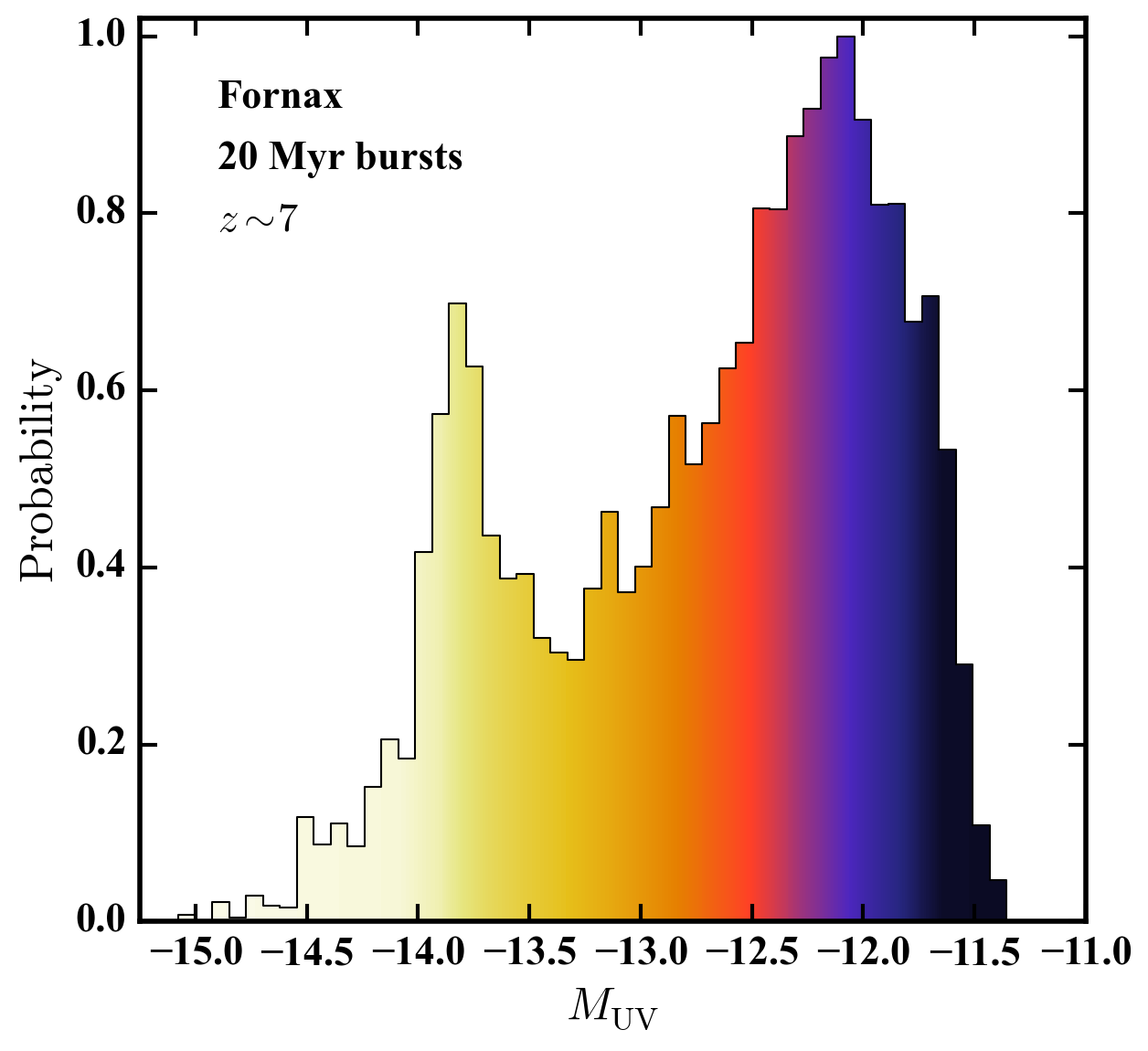
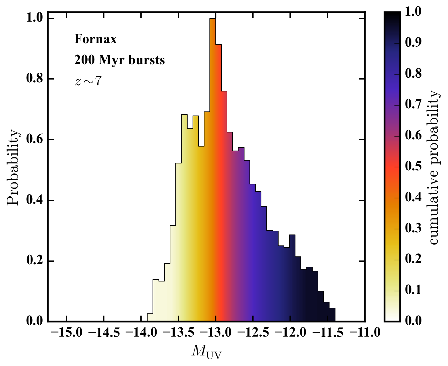
Figure 2: Probability distribution for ${M_{\rm UV}}$ of Fornax, given the photometric redshift distribution of Finkelstein et al. and assuming that Fornax’s high-redshift star formation occurred in bursts with a characteristic timescale of 20 Myr (left) or 200 Myr (right). The colors indicate the cumulative probability distribution in each panel. In the case of 20 Myr bursts, the frequent and relatively high-amplitude bursts result in a bimodal probability distribution function (with peaks corresponding to the burst and inter-burst periods). The 200 Myr bursts, which are modeled with smaller burst amplitudes, result in a distribution that is less broad and is unimodal. This is a direct consequence of our smaller assumed burst amplitude for 200 Myr bursts; the resulting SFH is therefore much closer to the fiducial constant SFH. Taking the instantaneous value of ${M_{\rm UV}}$ at $z=7$ in each realization results in a cumulative distribution that is very similar to that shown here in each case.

Figure 2 shows the probability distribution $P({M_{\rm UV}})$ for the Fornax dwarf spheroidal (dSph) galaxy, computed from 1000 realizations of its SFH, at $z\sim 7$. The left panel shows the case of 20 Myr bursts while the right panel shows the result for 200 Myr bursts. The distributions are shown as shaded histograms; the shading gives the value of the cumulative distribution function $P(<\!{M_{\rm UV}})$ for each ${M_{\rm UV}}$. Taking the instantaneous value of ${M_{\rm UV}}$ at $z=7$ in each realization results in a cumulative distribution that is very similar to that shown here in each case.

While the full range of ${M_{\rm UV}}$ spanned by the distributions is set by the burst fluctuation amplitude and is therefore roughly the same in the case of 20 or 200 Myr bursts, the distributions themselves differ substantially. 20 Myr bursts result in a bimodal distribution with a prominent peak $\sim 0.5$ magnitudes from the faint end of the distribution and a secondary peak $\sim 1.0$ magnitudes from the bright end of the distribution. The median value falls at $\sim 1$ magnitude from the faint end of the distribution. In the case of 200 Myr bursts, the distribution is noticeably different: there is a much stronger peak near the median of the distribution, with relatively high probabilities of being up to half a magnitude brighter or a magnitude fainter than the median value of ${M_{\rm UV}}$. The net result is that the median probability in the case of 200 Myr bursts is approximately 0.5 magnitudes brighter than in the (likely more realistic) case of 20 Myr bursts (e.g., Weisz et al. 2012). This is similar to the value of ${M_{\rm UV}}$ that would be obtained by assuming a constant SFR over the entire period to $z=5$, i.e., the parameters we adopt for 200 Myr bursts act mainly to distribute ${M_{\rm UV}}$ about the median value for the constant SFH.

Table 1: Observed $V$-band magnitudes of Local Group dwarfs (column 2), along with modeled UV magnitudes at $z\sim 2$ (column 3) and $z\sim 7$ (column 4). The ${M_{\rm UV}}$ values quoted in columns 3 and 4 are the medians of the probability distributions, while the errors are the minimum range containing 68% (95%) of the cumulative probability for ${M_{\rm UV}}$.

Name	$M_{\rm V}(z=0)$	${M_{\rm UV}}(z\sim 2)$	${M_{\rm UV}}(z\sim 7)$
Carina	$-9.1\pm 0.5$	$-8.3^{+0.6\,(2.4)}_{-1.6\,(2.0)}$	$-8.9^{+0.9\,(1.3)}_{-0.9\,(1.5)}$
CVn I	$-8.6\pm 0.2$	$-6.9^{+3.9\,(3.9)}_{-1.4\,(3.2)}$	$-9.5^{+0.9\,(0.9)}_{-0.6\,(1.6)}$
Draco	$-8.8\pm 0.3$	$-9.4^{+0.6\,(2.3)}_{-1.7\,(2.2)}$	$-9.2^{+0.9\,(0.9)}_{-0.5\,(1.4)}$
Fornax	$-13.4\pm 0.3$	$-12.1^{+0.9\,(0.9)}_{-0.6\,(1.6)}$	$-12.6^{+1.1\,(1.1)}_{-0.5\,(1.4)}$
IC 1613	$-15.2\pm 0.2$	$-12.6^{+0.6\,(1.6)}_{-1.2\,(1.8)}$	$-13.4^{+0.9\,(1.0)}_{-0.7\,(1.6)}$
Leo A	$-12.1\pm 0.2$	$-5.7^{+0.7\,(0.9)}_{-0.5\,(1.2)}$	$-10.5^{+1.0\,(1.0)}_{-0.6\,(1.3)}$
Leo I	$-12.0\pm 0.3$	$-5.1^{+0.9\,(0.9)}_{-2.2\,(4.5)}$	$-11.1^{+1.0\,(1.0)}_{-0.6\,(1.4)}$
Leo II	$-9.8\pm 0.3$	$-8.7^{+1.2\,(1.5)}_{-0.8\,(2.2)}$	$-8.8^{+0.7\,(0.7)}_{-0.5\,(1.5)}$
Leo T	$-8.0\pm 0.5$	$-1.5^{+0.4\,(0.8)}_{-0.4\,(0.8)}$	$-7.9^{+0.9\,(0.9)}_{-0.6\,(1.5)}$
LMC	$-18.1\pm 0.1$	$-15.6^{+0.8\,(0.9)}_{-0.6\,(1.6)}$	$-15.8^{+1.0\,(1.1)}_{-0.6\,(1.4)}$
Phoenix	$-9.9\pm 0.4$	$-9.0^{+1.0\,(1.0)}_{-0.6\,(1.5)}$	$-10.0^{+0.8\,(0.8)}_{-0.6\,(1.5)}$
Sagittarius	$-13.5\pm 0.3$	$-5.9^{+0.4\,(0.8)}_{-0.4\,(0.8)}$	$-12.3^{+0.9\,(0.9)}_{-0.5\,(1.5)}$
Sculptor	$-11.1\pm 0.5$	$-10.5^{+0.5\,(2.3)}_{-1.5\,(1.9)}$	$-11.2^{+0.6\,(1.3)}_{-1.2\,(1.3)}$
SMC	$-16.8\pm 0.2$	$-14.3^{+0.8\,(1.3)}_{-1.0\,(1.8)}$	$-14.1^{+0.4\,(1.3)}_{-1.2\,(1.2)}$
Ursa Minor	$-8.8\pm 0.5$	$-6.2^{+1.7\,(1.6)}_{-2.9\,(5.1)}$	$-8.9^{+1.0\,(1.0)}_{-0.6\,(1.5)}$

Given the expectations from observations and cosmological simulations, we adopt 20 Myr bursts as our default model for star formation and compute UV magnitudes from the resulting probability distribution derived from 100 independent realizations per galaxy. The results at $z\sim 2$ and $z\sim 7$ are listed in Table 1. We quote median values and confidence intervals comprising the minimum range in ${M_{\rm UV}}$ containing 68% and 95% of the cumulative probability. Since virtually all of the galaxies have $P({M_{\rm UV}})$ distributions that look like Figure 2, these ranges are usually asymmetric about the median.

An immediate connection that we can make between high redshifts and current-day quantities is to compare observed $V$-band magnitudes at $z=0$ with modeled values of ${M_{\rm UV}}(z=7)$. Such a comparison is shown in Figure 3. Perhaps unsurprisingly, there is a clear correlation between high-redshift UV luminosity and present-day $V$-band luminosity for the dwarf galaxies studied here. The slope of this correlation is $0.71$, indicating that the high-redshift UV luminosities span a narrower range than the $z=0$ $V$-band luminosities. While there is non-negligible scatter in this relation, which is related to the diverse early SFHs of the low-mass dwarfs in particular (e.g., figure 12 of Weisz et al. 2014a), the correlation is well-defined over the range of luminosities studied here. We caution against extrapolating this relation to significantly higher luminosities, as it is unlikely to remain linear indefinitely. The balance between ${M_{\rm UV}}(z\sim 7)$ and $M_{V}(z=0)$ is set by the stellar mass formed at early times versus over a galaxy’s lifetime, and very massive galaxies today have predominantly ancient stellar populations (Thomas et al., 2005), which is more similar to low-mass classical dSphs in the MW than to galaxies at intermediate mass (such as the MW itself).

For our sample of galaxies as a whole, ${M_{\rm UV}}(z=2)$ is reasonably well-correlated with ${M_{\rm UV}}(z=7)$ and with $M_{V}(z=0)$. There are notable exceptions, however, including Leo A, Leo I, Leo T, and Sagittarius. These galaxies show much lower UV luminosities at $z\sim 2$ than would be naively expected based on their present-day luminosities. The origin of this difference lies in the SFHs of these galaxies: while all of the galaxies in our sample have ancient ($z\sim 7$) star formation, the galaxies listed above appear to have gone through relatively quiescent phases at lower redshifts (see figure 7 of Weisz et al. 2014a). These periods of quiescence result in dramatically reduced UV luminosities at those times.

As discussed at the beginning of this section, we have only included a representative set of Local Group galaxies. They are mainly selected based on diversity in stellar mass and morphology at $z=0$, and all have the requirement of reaching below the oldest MSTO in order to provide the best possible constraints on the stellar mass formed by $z=5$. Future work analyzing the CMDs of newer, deep HST observations will enable us to include a more exhaustive sample of Local Group galaxies.

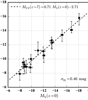
Figure 3: Observed $V$-band magnitude at $z=0$ versus modeled $z\sim 7$ UV magnitude. Error bars indicate minimum 68% confidence intervals (see Sec. 2.2 for more details). There is a well-defined, linear relation between the present-day $V$-band magnitude and the modeled high-redshift UV magnitude for the galaxies in our sample with a dispersion of $\sim 0.5$ magnitudes. The detailed form of this relation relies on the mode of star formation in galaxies. For the dwarf galaxies studied in this paper, we have assumed that star formation occurs predominantly in short-duration bursts. More massive galaxies are likely to maintain star formation over longer periods, which would result in a shallower relation between ${M_{\rm UV}}(z\sim 7)$ and $M_{\rm V}(z=0)$.

2.3 Uncertainties in, and limitations of, our approach

There are a number of assumptions we must make in our modeling. For completeness, we list several of them here.

• Star formation histories: we have only used the best-fit SFH, i.e., we assume perfect knowledge of the stellar mass at $z=5$. This is mitigated by the SFHs reaching the ancient MSTO, but it still can introduce uncertainties at the factor of $\la 2$ level into the total stellar mass formed.

• Aperture corrections: we assume the measured SFHs are representative of the entire galaxy. If the galaxies have strong population gradients, however, this assumption may be violated. The results of Hidalgo et al. (2013) indicate that at least some Local Group dwarf irregular galaxies do have population gradients, with younger stellar populations being more centrally concentrated than older populations. Any bias in our calculations is therefore likely to be in the direction of underestimating the UV luminosities at early times, as most of the galaxies have observations that sample close to their centers.

• Stellar IMF: we assume a fully populated Kroupa IMF, but the IMF may not be Kroupa or fully populated. Furthermore, we are basing the SFH on the IMF of lower-mass stars, but it was the high-mass stars in the early Universe that produced the UV light (Zaritsky et al., 2012).

• Dust: we do not make any corrections for dust in our modeling. This is unlikely to be a poor assumption for early-time progenitors of the Local Group dwarf galaxies we are considering, as the vast majority are very metal-poor even today. More massive, and vigorously star-forming, galaxies at the epoch of reionization may be dusty (see, e.g., Finkelstein et al. 2012; Watson et al. 2015). The galaxies studied here are expected to be low-metallicity and forming stars at rates of $10^{-4}-10^{-2}\,M_{\odot}\,{\rm yr^{-1}}$ at $z\sim 7$, however, and are likely to be dust-poor (Fisher et al., 2014).

• Metallicity: we assume a constant metallicity of $0.2\,Z_{\odot}$ throughout our analysis. Variations around this choice are unlikely to affect our modeling of ${M_{\rm UV}}$ appreciably; see Johnson et al. 2013 for further details and a more expansive discussion of several of the uncertainties discussed here.

• Distances: Our present analysis ignores the difference in luminosity distance over the width of photometric redshift distribution $P(z)$. For our $z=7$ sample, the distance modulus only varies by $\sim 0.2$ magnitudes from $z=6.5$ to $z=7.5$, meaning it will introduce at most a small correction to the effects we have modeled. The difference at $z\sim 2$ is $\sim 0.4$ magnitudes, which is still sub-dominant to the effects induced by bursty star formation.

One potentially important uncertainty is the merger histories of dwarf galaxies. Our approach is inherently archeological in nature, as we are using resolved SFHs of galaxies observed at $z=0$ to study the high-redshift Universe. Our analysis yields modeled UV fluxes as a function of time for the stars that are in the galaxy today, but those stars may have been formed in multiple distinct progenitors and only assembled more recently. If, for example, a typical merger history for our modeled galaxies were such that the $z=0$ galaxy had $N$ equal-mass progenitors at $z=7$, then our inferred UV luminosities at that epoch would be an overestimate by a factor of $N$. We assess the likely distribution of progenitor masses in two ways, through the use of abundance matching to dark-matter-only simulations (for a statistical understanding) and through high-resolution hydrodynamic simulations (for individual case studies).

Our first method relies on the ELVIS suite of dark-matter-only simulations of Local Group analogs (Garrison-Kimmel et al., 2014). We identify all objects within 1.2 Mpc of either Local Group giant at $z=0$ (excluding the central subhalos, which correspond to the MW and M31) and trace these objects back in time. Rather than following only the most massive progenitor, we track all progenitors at each previous redshift. We find that, at $z\sim 7$, there is typically a dominant progenitor in terms of mass: the next most massive progenitor is more than a factor of two lower in mass than the most massive progenitor at that epoch, on average. Based on our modeling, this indicates that the main progenitor is likely to be at least one magnitude brighter in the UV than any other progenitor. Since the SFHs are highly episodic, this statement is true only in a time-averaged sense.

We can also address this issue directly through hydrodynamical simulations. Specifically, we can use both an archeological and an instantaneous approach to $z\sim 7$ star formation by asking (1) how many of the stars in the galaxy at $z=0$ formed by $z=7$, and (2) what is the stellar content of the main progenitor of the $z=0$ galaxy at $z=7$? The difference between these two answers is a direct measure of the difference between resolved-star studies at $z=0$ and observations at $z\sim 7$. We use the cosmological zoom-in simulations described in Section 2.1 to perform this test. In all cases, the main progenitor of the simulated dwarf contains approximately 70% or more of the stars in the $z=0$ galaxy that have formed by $z=7$. The main progenitor is therefore already dominant by that time (see also Domínguez et al. 2014), and our archeological approach to the properties of Local Group galaxy progenitors at high redshift should be a reasonable approximation.

3 High-redshift observations in a Local Group context

With the results of Section 2, we are now in position to consider observations at high redshift in the context of well-observed galaxies in the Local Group. Of particular interest is the nature of the faintest objects observable in deep fields; in what follows, we discuss how the progenitors of Local Group dwarf galaxies would appear at $z\sim 7$ and $z\sim 2$.

3.1 Local Group galaxies at cosmic dawn

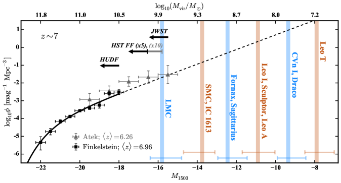
Figure 4: Local Group galaxies at $z\sim 7$. The data points show the observed UV luminosity function at $z\sim 7$ from Finkelstein et al. (2014; HST, no lensing; black squares) and Atek et al. (2015; HST Frontier Fields; gray triangles). The best-fit Schechter (1976) function ($M^{*}=-21.03,\,\phi^{*}=1.57\times 10^{-4}\,{\rm mag^{-1}\,Mpc^{-3}},\,\alpha=-2.03$) from Finkelstein et al. is displayed as a solid curve, while its extrapolation to lower luminosities is shown as a dashed line. The observational limits are also shown for the HUDF (assuming a completeness limit of ${M_{\rm UV}}=-18$), the HST Frontier Fields [assuming $m_{\rm lim}=28.7$ before lensing and a lensing magnification of 5 (1.75 magnitudes) or 10 (2.5 magnitudes)], and JWST (assuming $m_{\rm lim}=31.5$; this same depth would be reached in the Frontier Fields at $z=7$ with a magnification of 13.18 or 2.8 magnitudes). The modeled $\langle{M_{\rm UV}}(z\sim 7)\rangle$ for various Local Group galaxies are plotted as vertical bands (with error bars giving $1\,\sigma$ uncertainties; see Table 1), indicating the power of local observations for interpreting deep-field data. Consensus reionization models require extrapolation to ${M_{\rm UV}}(z\sim 7)\approx-13$, corresponding to the brightest dSphs today (Fornax, Sagittarius).

Figure 4 shows the observed UV LF of galaxies at $z\sim 7$ (from Finkelstein et al. 2014; see also McLure et al. 2013; Schenker et al. 2013; Schmidt et al. 2014; Bouwens et al. 2015b). The approximate halo masses expected for a given ${M_{\rm UV}}$ are shown on the upper horizontal axis; these are obtained by matching cumulative number densities of galaxies and halos (assuming a Sheth et al. (2001) mass function for the latter). In the deepest blank field, the HUDF, HST is capable of reaching ${M_{\rm UV}}\approx-17.5$. Models of reionization in which galaxies play the dominant role in maintaining an ionized intergalactic medium require a major contribution from fainter galaxies, however, meaning an important subset of the galaxies responsible for reionization have not yet been directly observed. The luminosities of the faintest galaxies contributing to reionization are unknown even theoretically, as this limit (often denoted $M_{\rm lim}$) depends on the slope of the UV LF and the escape fraction of ionizing photons from these galaxies (among other factors). The minimum ${M_{\rm UV}}$ necessary for maintaining reionization in models ranges from $M_{\rm lim}\approx-15$ to $M_{\rm lim}\ga-10$ (e.g., Kuhlen & Faucher-Giguère 2012; Robertson et al. 2013).

Our calculations of ${M_{\rm UV}}(z\sim 7)$ for Local Group galaxies can therefore provide crucial context for galaxies at cosmic dawn. We find that the progenitor of the Large Magellanic Cloud (LMC) – the brightest Local Group dwarf galaxy in our sample both at $z=0$ and $z\sim 7$– had ${M_{\rm UV}}(z\sim 7)\sim-16$, beyond the capabilities of HST in the HUDF. The Small Magellanic Cloud (SMC) and IC 1613 likely had ${M_{\rm UV}}(z=7)\sim-13.8$; virtually all reionization models therefore require progenitors of such galaxies to contribute to reionization. If ${M_{\rm UV}}(z\sim 7)\approx-13$ galaxies are required to maintain reionization, as is the case in many models, then the progenitors of the Sagittarius and Fornax dSphs must contribute. And finally, if galaxies as faint as ${M_{\rm UV}}(z\sim 7)\sim-9.5$ are required, then progenitors galaxies such as Draco, CVn I, and Phoenix – which have $L_{V}(z=0)\sim(0.2-1)\times 10^{6}\,L_{V,\odot}$ – may be necessary contributors to reionization.

These results also provide context for what observations in the HST Frontier Fields and with JWST will see. At $z\sim 7$, Frontier Fields can probe galaxies as faint as ${M_{\rm UV}}\approx-16.5$, assuming magnifications of 5 in luminosity (1.75 mags); such observations may approach the depth required for observing the main progenitor of the LMC. JWST deep field observations are expected to have a limiting magnitude of $m_{\rm AB}=31.5$ (Windhorst et al., 2006), corresponding to ${M_{\rm UV}}\sim-15.5$; JWST is therefore likely to reveal the $z\sim 7$ progenitors of Magellanic irregulars. If a Frontier Fields-like campaign with JWST could obtain a factor of 10 in magnification (2.5 mags), it would observe objects as faint as ${M_{\rm UV}}\approx-13$; this would just approach the sensitivity required to observe the progenitors of Fornax and Sagittarius, potentially revealing the faintest galaxies required for reionization. (We note that, based on the results of W14, we do not expect a strong truncation in the LF at at ${M_{\rm UV}}\sim-13$ or even at significantly fainter magnitudes; the idea of a limiting magnitude $M_{\rm lim}$ required for reionization is more of a mathematical construct than a physical cut-off. However, this does not preclude the possibility that the LF becomes shallower near $M_{\rm lim}$; see Sec. 3.1.) Progenitors of the vast majority of Local Group dwarfs will remain unobservable even with a JWST Frontier Fields-like project, however. This highlights the inherent difficulty of high-$z$ observations and the power of studying the high-$z$ Universe through its local descendants.

3.2 Near-field / deep-field connections

Figure 5: The $z=7$ mass function of the main progenitors of surviving $z=0$ (sub)halos – including the main progenitor of the MW itself – within 300 kpc of the Milky Way based on the ELVIS simulations (shaded region). The upper horizontal axis gives the abundance-matched ${M_{\rm UV}}$; the data points show our modeled UV luminosity function for progenitors of the MW and its satellites at $z\sim 7$. The luminosity function from direct modeling of SFHs and from abundance matching are in good agreement for ${M_{\rm UV}}\la-12.5$ ($M_{\rm{vir}}\approx 7\times 10^{8}\,M_{\odot}$) but diverge for fainter galaxies (lower mass halos), perhaps indicating the need for a break in the UV luminosity function at ${M_{\rm UV}}\approx-13$ at $z\sim 7$.

Figure 6: Similar to Figure 5, but assumes a UV luminosity function that breaks to $\alpha=-1.2$ at ${M_{\rm UV}}>-13$ (from the fiducial value of $\alpha=-2.03$ for brighter galaxies). The $z=7$ census of galaxies surviving to $z=0$ in the Milky Way is in much better agreement with the modeled UV luminosities in this case, as galaxies over a wider range in luminosity are placed in a narrower range of halo masses (for ${M_{\rm UV}}>-13$). In such a scenario, all known MW galaxies, including ultra-faint dwarfs, could lie at or above the atomic cooling threshold of $M_{\rm{vir}}\sim 10^{8}\,M_{\odot}$ at $z=7$.

Figure 4 indicates that the faintest galaxies observable in the HUDF at $z\sim 7$ likely are hosted by $M_{\rm{vir}}\approx 3\times 10^{10}\,M_{\odot}$ halos, while the atomic cooling threshold of $T_{\rm{vir}}\approx 10^{4}\,{\rm K}$ corresponds to ${M_{\rm UV}}\approx-10$. B14 showed that the ELVIS suite of simulated Local Groups predicts approximately 50 surviving, bound remnants of $M_{\rm{vir}}(z\sim 7)>10^{8}\,M_{\odot}$ halos in the Milky Way’s virial volume today. They argued this was potentially problematic, as even low-level star formation in such halos would quickly over-produce the observed stellar content of Milky Way satellites.

This tension is evident in Figure 5, which shows the $z\sim 7$ UV LF of the Milky Way and its satellites (symbols) as well as predicted dark matter halo mass functions from the ELVIS simulation suite (gray shaded region). The corresponding values of ${M_{\rm UV}}$ based on the abundance matching model described in Sec. 3.1 are given in the upper horizontal axis. The LF from direct modeling of SFHs and from abundance matching are in good agreement for ${M_{\rm UV}}\la-12$ ($M_{\rm{vir}}\approx 5\times 10^{8}\,M_{\odot}$), but the disagreement disappears for fainter galaxies (lower mass halos), with low-mass halos far outnumbering the number of known galaxies even at the modeled $z\sim 7$ luminosity of Draco and Leo II (${M_{\rm UV}}\sim-9$, corresponding to $M_{\rm halo}\sim 3\times 10^{7}\,M_{\odot}$). If every dark matter halo is capable of hosting a galaxy, then there should be 40-100 surviving descendants of galaxies with ${M_{\rm UV}}(z\sim 7)\la-10$; our modeling predicts there are only 10 or so such galaxies around the Milky Way today. Either only a small fraction of the halos at this mass ($M_{\rm halo}\approx 10^{8}\,M_{\odot}$) are capable of cooling gas and forming stars at $z\sim 7$ or the mapping between halo mass and UV luminosity is highly stochastic at early times in low-mass halos – both of which are contrary to current models and simulation results; or the UV LF breaks at ${M_{\rm UV}}\sim-13$, with $M_{\rm{vir}}\la 10^{9}\,M_{\odot}$ halos hosting fainter galaxies than our fiducial abundance matching model predicts. Whichever of these possibilities is correct, there are important implications for the threshold of galaxy formation and the mass scale of halos that host classical and ultra-faint dSphs.

The most realistic possibility may be that the $z\sim 7$ UV LF breaks at ${M_{\rm UV}}\approx-13$, as argued for in B14. Recent simulations have also found LFs that may flatten at fainter magnitudes than are probed by HST (Gnedin & Kaurov, 2014; O’Shea et al., 2015); there is no evidence for the LF flattening in current Frontier Fields data (Atek et al. 2015, Livermore et al. 2015, in preparation), which reach ${M_{\rm UV}}\sim-15.5$ at $z\sim 7$. ${M_{\rm UV}}\approx-13$ is also a frequently-adopted value of $M_{\rm lim}$ in models of reionization, although, as noted above, $M_{\rm lim}$ need not be associated with any feature or break in the UV LF.

If a break in the LF is indeed the answer, the Local Group data (in particular, galaxy counts at $z=0$ combined with modeled UV luminosities at $z\sim 7$) indicate the faint-end slope for ${M_{\rm UV}}\ga-13$ should be close to $-1.2$ rather than the value of approximately $-2$ that is observed in the HUDF. As is shown in Figure 6, fainter galaxies would then live in halos that are more massive than our original abundance matching prescription would indicate. This issue is explored in more detail, and at a variety of redshifts, in Graus et al. (in preparation). In this model (and in Fig. 6), the classical MW dSphs are hosted by halos with $M_{\rm{vir}}(z\sim 7)=(0.5-1)\times 10^{9}\,M_{\odot}$. All known Milky Way satellites could therefore be hosted by halos at or above the atomic cooling limit ($M_{\rm{vir}}\sim 10^{8}\,M_{\odot}$) at $z\sim 7$ (see also Milosavljević & Bromm 2014).

It is important to emphasize that completeness in the $z=0$ data is not an issue when constructing Figures 5-6: we have only used data for satellites with $L_{\rm V}(z=0)>10^{5}\,L_{V,\odot}$ and current Galactocentric distances of $<300\,{\rm kpc}$, a region where our census of satellites is very likely complete (e.g., Tollerud et al. 2008; Koposov et al. 2008; Walsh et al. 2009). Furthermore, the mismatch in Figure 5 is already significant for galaxies such as Leo I and Sculptor (with $L_{V}(z=0)\approx 5\times 10^{6}\,L_{V,\odot}$). The only galaxy this bright that has been found within the Milky Way’s virial volume since the 1950s is Sagittarius (Ibata et al., 1995), whose presence had been concealed by the Galaxy’s disk. Although we do not have data for Sextans, the discrepancy in numbers shown in Figure 5 is an order of magnitude, indicating that even the inclusion of Sextans and the discovery of several $10^{5}\,L_{V,\odot}$ satellites would not change the qualitative picture described here.

3.3 Local Group galaxies at cosmic noon

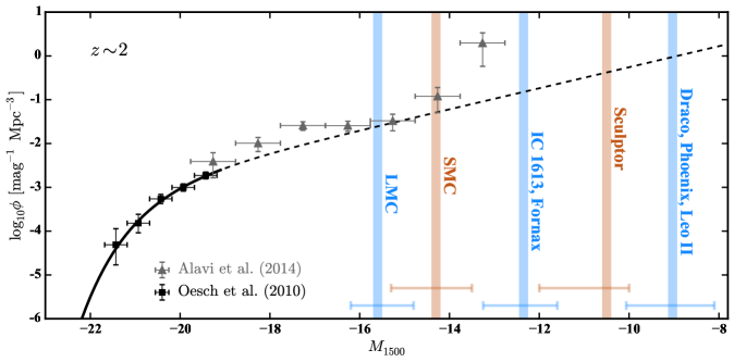
Figure 7: Local Group galaxies in a $z\sim 2$ context. The data points show HST observations of $z\sim 2$ galaxies in the GOODS-South field (Oesch et al. 2010; black points) and in the A1689 lensing field (Alavi et al. 2014; gray points). The best-fitting Schechter luminosity function from Oesch et al. $(M^{*}=-20.16,\,\phi^{*}=2.188\times 10^{-3}\,{\rm mag^{-1}\,Mpc^{-3}},\,\alpha=-1.60)$ is plotted as a solid curve, and its extrapolation to fainter magnitudes is plotted a dashed curve. Vertical bands indicate the modeled $\langle{M_{\rm UV}}(z\approx 2)\rangle$ for various Local Group galaxies (with error bars giving $1\,\sigma$ uncertainties; see Table 1). While deep observations of blank fields only probe much more massive galaxies than those of the Local Group (except the Galaxy and M31), lensing magnification likely enables the study of galaxies similar to progenitors of the LMC and SMC at $z\sim 2$ and are nearly capable of reaching the main progenitor of galaxies like IC 1613 and Fornax at that time.

Dwarf galaxies are also important test-beds of galaxy formation physics at eras other than the epoch of reionization. In particular, large samples of UV-selected galaxies at $z\sim 2$ are becoming available, and ongoing HST programs are enabling studies of galaxies that are intrinsically as faint as ${M_{\rm UV}}\sim-13.5$ (Alavi et al., 2014) at that time, which is close to “cosmic noon”, the peak of the cosmic star formation rate density (Madau & Dickinson, 2014). Understanding the likely descendants of such galaxies today – or the likely progenitors of Local Group galaxies – will shed further light on the processes at work in galaxy formation over the past 10 billion years.

Figure 7 shows the observed UV LF of galaxies at $z\sim 2$ (black data points, from Oesch et al. 2010). The gray data points are observations that take advantage of lensing magnification combined with deep near-UV imaging (WFC3/UVIS in F275W), which allowed Alavi et al. to probe to much fainter galaxies (${M_{\rm UV}}\sim-13$) than would otherwise be possible. The figure also shows the UV magnitudes that a variety of Local Group galaxies would have at this redshift.

The LMC and SMC are predicted to have ${M_{\rm UV}}(z\sim 2)\approx-16$ and $-14$, respectively, placing them well within the reach of HST at $z\sim 2$. IC 1613 and the Fornax dSph are predicted to have ${M_{\rm UV}}(z\sim 2)\approx 12.5$, meaning the progenitors of these galaxies are just at the edge of HST’s current capabilities at $z=2$. Other Local Group galaxies in our sample are all predicted to be fainter than ${M_{\rm UV}}=-12$ at $z\sim 2$.

As yet larger samples of galaxies become available, it will be possible to examine $z\sim 2$ galaxies as a population in ever-greater detail. If lensing allows the study of ${M_{\rm UV}}\sim-12$ galaxies at $z\sim 2$, a number of applications will present themselves. Such observations will likely reveal the progenitors of present-day dwarf irregular galaxies and massive dSphs in a variety of environments. The distribution of $z\sim 2$ UV fluxes obtained through direct observation will help constrain potential burst parameters (e.g., the $z\sim 2$ equivalent of Figure 2). Observations at $z\sim 2$ will also increase the precision with which the faint end slope of the UV luminosity function can be measured, placing further constraints on the evolution of cosmic star formation and on the properties of dust in faint, star-forming galaxies.

4 Discussion

The previous sections illustrate the power that deep resolved-star observations of Local Group galaxies have for understanding not just the nearby Universe but also (much) earlier eras. Using the modeled UV luminosities, we have shown that Local Group galaxies such as the Fornax dSph and IC 1613 were, at $z\sim 2$, slightly less luminous (${M_{\rm UV}}\sim-12.5$) than the faintest galaxies HST is currently observing at that epoch (${M_{\rm UV}}\sim-13$). The LMC and SMC are predicted to be substantially more luminous at that time; many of the faint (${M_{\rm UV}}\sim-15$) galaxies observed at $z\sim 2$ may evolve to become Magellanic irregulars in the local Universe. Pushing to higher redshifts ($z\sim 7$), we find that none of the Local Group galaxies are bright enough to be seen in the HUDF, consistent with expectations based on number counts and space densities (e.g., Trenti et al. 2010, B14). Many reionization models predict that extrapolating the observed LF to ${M_{\rm UV}}\sim-10$ is required to maintain reionization; if this is the case, the progenitors of some of the faintest classical dSphs (e.g., Draco, CVn I) and low-luminosity dwarf irregulars (e.g., Phoenix and Leo A) would be required contributors to the ionizing background.

In Section 3.2, we showed that a comparison between our derived ${M_{\rm UV}}$ values for Local Group galaxies at $z\sim 7$ and counts of surviving subhalos in dark-matter-only simulations of the Local Group show that $z\sim 7$ LF cannot continue with a slope of $\alpha=-2$ to ${M_{\rm UV}}\sim-9$, as this would imply an order-of-magnitude excess in surviving satellites with $z=0$ luminosities comparable to the classical MW dwarfs. The faint-end slope derived from high-$z$ observations is still somewhat degenerate with measured value of $M^{*}$ in the Schechter LF, however, with a typical uncertainty of $\pm 0.3$ (e.g., McLure et al. 2013; Finkelstein et al. 2014; Bouwens et al. 2015b). These degeneracies translate into substantial uncertainties in $M_{\rm lim}$ (see, e.g., figure 2 of Robertson et al. 2013), which in turn will affect the specific value of ${M_{\rm UV}}$ at which archeological studies in the MW require the high-$z$ LF to break. The general trend is that if the faint-end slope of the LF is steeper, it must break at brighter values of ${M_{\rm UV}}$; if it is shallower, the break can occur at fainter values. This mirrors the behavior of $M_{\rm lim}$ and its dependence on $\alpha$.

The Planck collaboration has recently reported a value of the optical depth to electron scattering, $\tau=0.066\pm 0.012$ (Planck Collaboration, 2015), that is $\approx 30\%$ lower than previous determinations of $\tau=0.088\pm 0.014$ (Komatsu et al., 2011). Robertson et al. (2015) show that extrapolating the LF to a limiting magnitude of $M_{\rm lim}\approx-13$ (with a luminosity-independent escape fraction $f_{\rm esc}=0.2$) is sufficient to maintain reionization (see also Finkelstein et al. 2012) and match the updated Planck determination of $\tau$. Such a scenario still requires extrapolation of the LF down to progenitors of the Fornax dSph, which has a present-day luminosity of $L_{V}\approx 10^{7}\,L_{V,\odot}$.

If time-averaged escape fractions are lower than 20% for galaxies with ${M_{\rm UV}}\la-13$, as suggested by the work of Wise et al. (2014) and Ma et al. (2015), then maintaining reionization would require even fainter galaxies (or additional sources such as X-rays; e.g., Mirabel et al. 2011). Galaxy-driven reionization scenarios therefore still require that most of the known Local Group irregular galaxies – and the most luminous of the dSphs – were necessary contributors to cosmic reionization. These galaxies are intrinsically very faint at high redshift: JWST will only resolve galaxies that are an order-of-magnitude brighter even in a deep field campaign. The unique high-angular-resolution capabilities of observatories such as HST and JWST, and the deep observations of faint galaxies in and around the Local Group they facilitate, therefore hold the promise of providing a unique probe of the earliest epoch of galaxy formation.

References

- Alavi et al. (2014) Alavi, A. et al. 2014, ApJ, 780, 143
- Alvarez et al. (2012) Alvarez, M. A., Finlator, K., & Trenti, M. 2012, ApJ, 759, L38
- Atek et al. (2015) Atek, H. et al. 2015, ApJ, 800, 18
- Benítez-Llambay et al. (2015) Benítez-Llambay, A., Navarro, J. F., Abadi, M. G., Gottlöber, S., Yepes, G., Hoffman, Y., & Steinmetz, M. 2015, MNRAS, 450, 4207
- Bouwens et al. (2015a) Bouwens, R. J., Illingworth, G. D., Oesch, P. A., Caruana, J., Holwerda, B., Smit, R., & Wilkins, S. 2015a, arXiv:1503.08228 [astro-ph]
- Bouwens et al. (2015b) Bouwens, R. J. et al. 2015b, ApJ, 803, 34
- Bouwens et al. (2012) —. 2012, ApJ, 752, L5
- Bovill & Ricotti (2011) Bovill, M. S., & Ricotti, M. 2011, ApJ, 741, 17
- Boylan-Kolchin et al. (2014) Boylan-Kolchin, M., Bullock, J. S., & Garrison-Kimmel, S. 2014, MNRAS, 443, L44
- Brown et al. (2012) Brown, T. M. et al. 2012, ApJ, 753, L21
- Bullock et al. (2000) Bullock, J. S., Kravtsov, A. V., & Weinberg, D. H. 2000, ApJ, 539, 517
- Cole et al. (2007) Cole, A. A. et al. 2007, ApJ, 659, L17
- Conroy & Gunn (2010) Conroy, C., & Gunn, J. E. 2010, ApJ, 712, 833
- Conroy et al. (2009) Conroy, C., Gunn, J. E., & White, M. 2009, ApJ, 699, 486
- Dolphin (2002) Dolphin, A. E. 2002, MNRAS, 332, 91
- Domínguez et al. (2014) Domínguez, A., Siana, B., Brooks, A. M., Christensen, C. R., Bruzual, G., Stark, D. P., & Alavi, A. 2014, arXiv:1408.5788 [astro-ph]
- Duffy et al. (2014) Duffy, A. R., Wyithe, J. S. B., Mutch, S. J., & Poole, G. B. 2014, MNRAS, 443, 3435
- Dunlop et al. (2013) Dunlop, J. S. et al. 2013, MNRAS, 432, 3520
- Finkelstein et al. (2012) Finkelstein, S. L. et al. 2012, ApJ, 758, 93
- Finkelstein et al. (2014) —. 2014, arXiv:1410.5439 [astro-ph]
- Fisher et al. (2014) Fisher, D. B. et al. 2014, Nature, 505, 186
- Freeman & Bland-Hawthorn (2002) Freeman, K., & Bland-Hawthorn, J. 2002, ARA&A, 40, 487
- Garrison-Kimmel et al. (2014) Garrison-Kimmel, S., Boylan-Kolchin, M., Bullock, J. S., & Lee, K. 2014, MNRAS, 438, 2578
- Girardi et al. (2002) Girardi, L., Bertelli, G., Bressan, A., Chiosi, C., Groenewegen, M. A. T., Marigo, P., Salasnich, B., & Weiss, A. 2002, A&A, 391, 195
- Girardi et al. (2010) Girardi, L. et al. 2010, ApJ, 724, 1030
- Gnedin & Kaurov (2014) Gnedin, N. Y., & Kaurov, A. A. 2014, ApJ, 793, 30
- Governato et al. (2012) Governato, F. et al. 2012, MNRAS, 422, 1231
- Hidalgo et al. (2013) Hidalgo, S. L. et al. 2013, ApJ, 778, 103
- Hopkins (2015) Hopkins, P. F. 2015, MNRAS, 450, 53
- Hopkins et al. (2014) Hopkins, P. F., Kereš, D., Oñorbe, J., Faucher-Giguère, C.-A., Quataert, E., Murray, N., & Bullock, J. S. 2014, MNRAS, 445, 581
- Hunter (2007) Hunter, J. D. 2007, Computing In Science & Engineering, 9, 90
- Ibata et al. (1995) Ibata, R. A., Gilmore, G., & Irwin, M. J. 1995, MNRAS, 277, 781
- Johnson et al. (2013) Johnson, B. D. et al. 2013, ApJ, 772, 8
- Jones et al. (2001) Jones, E., Oliphant, T., Peterson, P., et al. 2001, SciPy: Open source scientific tools for Python, [Online; accessed 2015-02-15]
- Kauffmann (2014) Kauffmann, G. 2014, MNRAS, 441, 2717
- Komatsu et al. (2011) Komatsu, E. et al. 2011, ApJS, 192, 18
- Koposov et al. (2008) Koposov, S. et al. 2008, ApJ, 686, 279
- Kroupa (2001) Kroupa, P. 2001, MNRAS, 322, 231
- Kuhlen & Faucher-Giguère (2012) Kuhlen, M., & Faucher-Giguère, C.-A. 2012, MNRAS, 423, 862
- Ma et al. (2015) Ma, X., Kasen, D., Hopkins, P. F., Faucher-Giguere, C.-A., Quataert, E., Keres, D., & Murray, N. 2015, arXiv:1503.07880 [astro-ph]
- Madau & Dickinson (2014) Madau, P., & Dickinson, M. 2014, ARA&A, 52, 415
- Madau et al. (2008) Madau, P., Kuhlen, M., Diemand, J., Moore, B., Zemp, M., Potter, D., & Stadel, J. 2008, ApJ, 689, L41
- Madau et al. (2014) Madau, P., Weisz, D. R., & Conroy, C. 2014, ApJ, 790, L17
- McConnachie (2012) McConnachie, A. W. 2012, AJ, 144, 4
- McLure et al. (2013) McLure, R. J. et al. 2013, MNRAS, 432, 2696
- Milosavljević & Bromm (2014) Milosavljević, M., & Bromm, V. 2014, MNRAS, 440, 50
- Mirabel et al. (2011) Mirabel, I. F., Dijkstra, M., Laurent, P., Loeb, A., & Pritchard, J. R. 2011, A&A, 528, A149
- Oñorbe et al. (2015) Oñorbe, J., Boylan-Kolchin, M., Bullock, J. S., Hopkins, P. F., Kerěs, D., Faucher-Giguère, C.-A., Quataert, E., & Murray, N. 2015, arXiv:1502.02036 [astro-ph]
- Oesch et al. (2010) Oesch, P. A. et al. 2010, ApJ, 725, L150
- O’Shea et al. (2015) O’Shea, B. W., Wise, J. H., Xu, H., & Norman, M. L. 2015, arXiv:1503.01110 [astro-ph]
- Pérez & Granger (2007) Pérez, F., & Granger, B. E. 2007, Computing in Science and Engineering, 9, 21
- Planck Collaboration (2015) Planck Collaboration. 2015, arXiv:1502.01589 [astro-ph]
- Power et al. (2014) Power, C., Wynn, G. A., Robotham, A. S. G., Lewis, G. F., & Wilkinson, M. I. 2014, arXiv:1406.7097 [astro-ph]
- Ricotti & Gnedin (2005) Ricotti, M., & Gnedin, N. Y. 2005, ApJ, 629, 259
- Ricotti et al. (2008) Ricotti, M., Gnedin, N. Y., & Shull, J. M. 2008, ApJ, 685, 21
- Robertson et al. (2015) Robertson, B. E., Ellis, R. S., Furlanetto, S. R., & Dunlop, J. S. 2015, ApJ, 802, L19
- Robertson et al. (2013) Robertson, B. E. et al. 2013, ApJ, 768, 71
- Salvaterra et al. (2011) Salvaterra, R., Ferrara, A., & Dayal, P. 2011, MNRAS, 414, 847
- Schechter (1976) Schechter, P. 1976, ApJ, 203, 297
- Schenker et al. (2013) Schenker, M. A. et al. 2013, ApJ, 768, 196
- Schmidt et al. (2014) Schmidt, K. B. et al. 2014, ApJ, 786, 57
- Sheth et al. (2001) Sheth, R. K., Mo, H. J., & Tormen, G. 2001, MNRAS, 323, 1
- Skillman et al. (2014) Skillman, E. D. et al. 2014, ApJ, 786, 44
- Stinson et al. (2007) Stinson, G. S., Dalcanton, J. J., Quinn, T., Kaufmann, T., & Wadsley, J. 2007, ApJ, 667, 170
- Teyssier et al. (2013) Teyssier, R., Pontzen, A., Dubois, Y., & Read, J. I. 2013, MNRAS, 429, 3068
- Thomas et al. (2005) Thomas, D., Maraston, C., Bender, R., & Mendes de Oliveira, C. 2005, ApJ, 621, 673
- Tollerud et al. (2008) Tollerud, E. J., Bullock, J. S., Strigari, L. E., & Willman, B. 2008, ApJ, 688, 277
- Trenti et al. (2010) Trenti, M., Stiavelli, M., Bouwens, R. J., Oesch, P., Shull, J. M., Illingworth, G. D., Bradley, L. D., & Carollo, C. M. 2010, ApJ, 714, L202
- Van Der Walt et al. (2011) Van Der Walt, S., Colbert, S. C., & Varoquaux, G. 2011, arXiv:1102.1523 [astro-ph]
- van der Wel et al. (2011) van der Wel, A. et al. 2011, ApJ, 742, 111
- Vogelsberger et al. (2014) Vogelsberger, M., Zavala, J., Simpson, C., & Jenkins, A. 2014, MNRAS, 444, 3684
- Walsh et al. (2009) Walsh, S. M., Willman, B., & Jerjen, H. 2009, AJ, 137, 450
- Watson et al. (2015) Watson, D., Christensen, L., Knudsen, K. K., Richard, J., Gallazzi, A., & Michałowski, M. J. 2015, Nature, 519, 327
- Weisz et al. (2013) Weisz, D. R., Dolphin, A. E., Skillman, E. D., Holtzman, J., Dalcanton, J. J., Cole, A. A., & Neary, K. 2013, MNRAS, 431, 364
- Weisz et al. (2014a) Weisz, D. R., Dolphin, A. E., Skillman, E. D., Holtzman, J., Gilbert, K. M., Dalcanton, J. J., & Williams, B. F. 2014a, ApJ, 789, 147
- Weisz et al. (2014b) Weisz, D. R., Johnson, B. D., & Conroy, C. 2014b, ApJ, 794, L3
- Weisz et al. (2012) Weisz, D. R. et al. 2012, ApJ, 744, 44
- Wheeler et al. (2015) Wheeler, C., Onorbe, J., Bullock, J. S., Boylan-Kolchin, M., Elbert, O., Garrison-Kimmel, S., Hopkins, P. F., & Keres, D. 2015, arXiv:1504.02466 [astro-ph]
- Windhorst et al. (2006) Windhorst, R. A., Cohen, S. H., Jansen, R. A., Conselice, C., & Yan, H. 2006, New Astron. Rev., 50, 113
- Wise et al. (2014) Wise, J. H., Demchenko, V. G., Halicek, M. T., Norman, M. L., Turk, M. J., Abel, T., & Smith, B. D. 2014, MNRAS, 442, 2560
- Zaritsky et al. (2012) Zaritsky, D., Colucci, J. E., Pessev, P. M., Bernstein, R. A., & Chandar, R. 2012, ApJ, 761, 93
- Zolotov et al. (2012) Zolotov, A. et al. 2012, ApJ, 761, 71