Matrix product state representation of non-Abelian quasiholes

Abstract

We provide a detailed explanation of the formalism necessary to construct matrix product states for non-Abelian quasiholes in fractional quantum Hall model states. Our construction yields an efficient representation of the wave functions with conformal-block normalization and monodromy, and complements the matrix product state representation of fractional quantum Hall ground states.

I Introduction

The fractional quantum Hall (FQH) effect Tsui et al. (1982) is the archetypal system for the emergence of topological order Wen (1995) in condensed matter physics. Due to the presence of strong correlations, the theoretical understanding of its microscopic properties heavily relies on finite-size numerics. Laughlin (1983); Haldane (1983); Tserkovnyak and Simon (2003); Prodan and Haldane (2009); Baraban et al. (2009) Such calculations are limited to rather small system sizes, as the many-body Hilbert space grows exponentially with the system area. An ingenious way to circumvent this problem comes from the recent development Dubail et al. (2012); Zaletel and Mong (2012); Estienne et al. (2013a, b); Wu et al. (2014); Estienne et al. (2015); Zaletel et al. (2013) of exact matrix product states Fannes et al. (1992); Schollwöck (2011) (MPS) for a large class of FQH model wave functions derived from conformal field theory (CFT) correlators Belavin et al. (1984); Fubini (1991); Moore and Read (1991). Exploiting the area law of quantum entanglement, Eisert et al. (2010) the MPS factorization enables efficient calculation of physical observables and gives access to much larger system sizes than previously attainable.

In a recent paper, Wu et al. (2014) we applied this technique to study quasihole excitations in the Moore-Read, Moore and Read (1991) the Gaffnian, Simon et al. (2007) and the $\mathbb{Z}_{3}$ Read-Rezayi Read and Rezayi (1999) states. These exotic quasiparticles were conjectured to be non-Abelian anyons, and they constitute the most striking manifestation of the topological order in the FQH liquids. Kitaev (2003); Nayak et al. (2008) A hallmark of their non-Abelian character lies in the topological degeneracy of multiquasihole states. For each set of fixed quasihole positions, there exists a quasidegenerate subspace of states, protected against local perturbations, and braiding the quasiholes induces unitary transformations over this degenerate subspace. These transformations depend only on the topology of the braids, rather than their actual shapes, and those induced by distinct braids do not commute. In Ref. Wu et al., 2014, using the MPS representation, we explicitly demonstrated for the first time the Fibonacci nature of the $\mathbb{Z}_{3}$ Read-Rezayi quasiholes from a microscopic calculation. We estimated the quasihole radii and quantified the length scales associated with the exponential convergence of the braiding statistics, but did not provide details regarding the construction of the quasihole wavefunctions. In this paper, we discuss in detail the novel technical aspects of the MPS representation for the non-Abelian quasiholes.

The construction of the exact MPS is based on the rewriting of FQH model wave functions as conformal correlators. Fubini (1991); Moore and Read (1991) This elegant formalism provides a particularly nice way to resolve the topological degeneracy of non-Abelian quasiholes Moore and Read (1991) in terms of the so-called conformal blocks. Moore and Seiberg (1989); Di Francesco et al. (1997) Each conformal-block wave function is indexed not only by the quasihole positions, but also by a tree of topological charge labels specifying the different fusion channels of the quasiholes. Enumerating all the possible fusion tree labelings compatible with a given theory generates a complete basis over the degenerate subspace. A special benefit of the conformal-block basis is the explicit manifestation of the putative braiding statistics in the analytic structure of the wave functions. Nayak and Wilczek (1996); Ardonne and Schoutens (2007) Specifically, as a function of the complex quasihole coordinates, the conformal blocks display branch-cut singularities emanating from the quasihole centers. The monodromy matrix associated with crossing the branch cuts is conjectured Moore and Read (1991) to coincide with the corresponding quasihole braiding matrix, up to an Abelian Aharonov-Bohm phase due to the magnetic field. This conjecture rests on the observation that the overlaps between conformal blocks resemble the partition function of a classical plasma Laughlin (1983) with pinned quasihole charges, a peculiar feature of the quasihole-dependent normalization of the conformal blocks. Arovas et al. (1984) This link eliminates the need to directly integrate the non-Abelian Berry connection to compute the braiding matrix. Gurarie and Nayak (1997); Read (2009); Bonderson et al. (2011) To demonstrate that the braiding statistics is indeed captured by the monodromy of conformal blocks, we only have to establish (through a microscopic calculation) that the plasma is in a screening phase. This simplification led to the analytic identification (with the assumption of plasma screening) of the Moore-Read quasiholes as Ising anyons in Ref. Bonderson et al., 2011, and also played a crucial role in our numerical demonstration Wu et al. (2014) of the $\mathbb{Z}_{3}$ Read-Rezayi quasiholes as Fibonacci anyons. The main purpose of the current paper is to explain how to translate the conformal blocks into calculation-friendly MPS form while preserving the two highly desirable features, namely, the monodromy structure and the plasma normalization.

The paper is organized as follows. In Sec. II, we provide a pedagogical review on the construction of quantum Hall MPS in the absence of non-Abelian quasiholes, and in particular, we derive the plasma normalization from conformal correlators on the cylinder. And as a precursor, we also discuss the MPS representation of Abelian quasiholes. In Sec. III we proceed to the non-Abelian case. We explain step by step how to construct MPS for the conformal-block wave functions with quasiholes in the bulk. A large part of the discussion is devoted to the derivation of the subtle commutation rules between a non-Abelian quasihole insertion and the electron operators. We provide explicit recipes for the Moore-Read, Moore and Read (1991) the Gaffnian, Simon et al. (2007), and the $\mathbb{Z}_{3}$ Read-Rezayi Read and Rezayi (1999) states. Technical details of the construction are addressed in the appendices.

II Matrix product states from conformal correlators

Before discussing the non-Abelian quasiholes, we first review the construction Dubail et al. (2012); Zaletel and Mong (2012); Estienne et al. (2013a, b) of the quantum Hall matrix product states (MPS) from conformal correlators. In preparation for the later discussion of the quasihole wave functions, we pay special attention to preserving the normalization of the conformal correlator.

We consider model wave functions in the lowest Landau level constructed from chiral conformal correlators. Fubini (1991); Moore and Read (1991) In this formalism, an electron at position $z$ is represented by a primary field insertion $\mathcal{V}(z)$, and the conformal correlator

$$\Big{\langle}\mathcal{V}(z_{1})\mathcal{V}(z_{2})\cdots\mathcal{V}(z_{n})\Big{\rangle}$$ (1)

can be viewed as a many-body wave function $\Psi(z_{1},z_{2},\ldots,z_{n})$. Here and hereafter, the single brackets $\langle\,\cdot\,\rangle$ denote a CFT correlation function, in contrast to the double brackets $\langle\!\langle\,\cdot\,\rangle\!\rangle$ representing the states (wave functions) of the physical electrons. For example, the Laughlin wave function Laughlin (1983) at filling $\nu$ can be described Fubini (1991) in terms of a massless free boson $\phi$. The electron operator $\mathcal{V}(z)$ is the normal-ordered exponential

$$\mathcal{V}(z)=\,:\!e^{i\frac{1}{\sqrt{\nu}}\phi(z)}\!:.$$ (2)

Using the propagator ${\langle\phi(z)\phi(z^{\prime})\rangle=-\log(z-z^{\prime})}$ in the plane, we recover from Eq. (1) the familiar Laughlin wave function ${\prod_{i<j}(z_{i}-z_{j})^{1/\nu}}$. For more complicated quantum Hall states (see Sec. III), the corresponding CFT has a direct-product structure, Moore and Read (1991) where in addition to the free boson, we also have a separate so-called “neutral” CFT.

From now on we adopt the cylinder geometry Rezayi and Haldane (1994) with finite perimeter $L_{y}$. The complex coordinate ${z=x+iy}$ has $x$ running along the cylinder axis and $y$ around its perimeter. For convenience, we set the magnetic length to unity, and we define the inverse cylinder radius

$$\gamma=\frac{2\pi}{L_{y}}.$$ (3)

The many-body wave function $\Psi(z_{1},z_{2},\ldots,z_{n})$ is given by the conformal correlator in Eq. (1) evaluated in the cylinder geometry, which can be mapped the usual planar geometry through the conformal transformation $z\rightarrow e^{\gamma z}$.

Interpreting the $x$ coordinate as the imaginary time, the CFT Hamiltonian is given by $\gamma(\hat{L}_{0}-\frac{1}{24}c)$, with $\hat{L}_{0}$ being the Virasoro generator for dilations and $c$ being the chiral central charge. For the direct-product theory of a neutral CFT and a free boson, we have the decomposition

$$\hat{L}_{0}=\hat{L}_{0}^{\text{neut}}+\hat{L}_{0}^{\text{boson}}.$$ (4)

In this section, we focus on the boson part. The mode expansion of the chiral field $\phi$ on the cylinder is given by

$$\phi(z)=\hat{\phi}_{0}-i\gamma z\,\hat{a}_{0}+i\sum_{n\neq 0}\frac{1}{n}\,\hat{a}_{n}e^{-n\gamma z}.$$ (5)

Here, the $\hat{a}_{n}$ modes of the U(1) current satisfy the Heisenberg algebra

$$[\hat{a}_{n},\hat{a}_{m}]=n\,\delta_{n+m,0},$$ (6)

while $\hat{\phi}_{0}$ is the canonical conjugate to the zero mode $\hat{a}_{0}$,

$$[\hat{\phi}_{0},\hat{a}_{0}]=i.$$ (7)

And the dilation operator for the free boson is given by

$$\hat{L}_{0}^{\text{boson}}=\sum_{m>0}\hat{a}_{-m}\hat{a}_{m}+\frac{1}{2}\hat{a}_{0}^{2}.$$ (8)

The $\hat{a}_{0}$ operator measures the U(1) charge in unit of $\sqrt{\nu}$ times the electron charge, in the sense that

$$[\mathcal{V}(z)]^{-1}\,\hat{a}_{0}\,\mathcal{V}(z)=\hat{a}_{0}+\frac{1}{\sqrt{\nu}}.$$ (9)

The zero mode operators $\hat{\phi}_{0}$ and $\hat{a}_{0}$ are decoupled from (commute with) the ladder operators $\hat{a}_{n\neq 0}$. As a result, the free boson Hilbert space can be split into sectors labeled by the U(1) charge $\hat{a}_{0}$, with $\hat{\phi}_{0}$ coupling different sectors. The primary state $|Q\rangle={:\!e^{iQ\hat{\phi}_{0}}\!:}|\mathbbm{1}\rangle$ has U(1) charge $Q$, and the corresponding Hilbert space sector with charge $Q$ is spanned by the descendants of $|Q\rangle$ under the boson modes $\{\hat{a}_{n<0}\}$.

II.1 Background charge and gauge choice

The MPS is a tensor factorization of the second-quantized amplitudes of the many-body wave function $\Psi(z_{1},z_{2},\ldots,z_{N})$ in Eq. (1). Dubail et al. (2012); Zaletel and Mong (2012) The first step of the construction is to obtain $\Psi$ in the occupation-number basis. We choose the Landau gauge for the magnetic field, and work with the orbitals labeled by the wave number $j\in\mathbb{Z}$ in the $y$ direction:

$$\psi_{j}(x,y) =\frac{1}{(\sqrt{\pi}L_{y})^{\frac{1}{2}}}\,e^{i\gamma jy}e^{-\frac{1}{2}(x-\gamma j)^{2}}$$ (10)

$$=\frac{e^{-\frac{1}{2}\gamma^{2}j^{2}}}{(\sqrt{\pi}L_{y})^{\frac{1}{2}}}\,e^{\gamma jz}e^{-\frac{1}{2}x^{2}}.$$

These one-body states take the form of a holomorphic function in $z$ times a Gaussian in $x$. Due to the chirality of the electron operators $\mathcal{V}(z)$, the conformal correlator in Eq. (1) does not produce the (non-holomorphic) Gaussian factor, and thus does not yet qualify as a many-body wave function in the lowest Landau level (in any gauge). Fortunately, the Gaussian factor can be generated naturally by spreading the neutralizing background charge for the boson field $\phi$ uniformly Moore and Read (1991) on the cylinder. This amounts to inserting another (non-primary) field

$$\mathcal{O}_{\text{bc}}=\,\,:\!\exp\left(-i\frac{\sqrt{\nu}}{2\pi}\int\mathrm{d}^{2}w\,\,\phi(w)\right)\!:$$ (11)

into the conformal correlator, representing the neutralizing background charge at filling $\nu$. Here, the integration is performed over the cylinder surface, and the normal ordering removes unwanted interactions between background charges at different locations. However, as discussed in Ref. Moore and Read, 1991, this extra insertion of the background charge has a side effect: in addition to the desirable Gaussian factor, it also introduces a non-holomorphic gauge factor. Taken altogether, the cylinder many-body wave function in the Landau gauge is given by Zaletel and Mong (2012)

$$\Psi(z_{1},\ldots,z_{n})=e^{i\sum_{i}x_{i}y_{i}}\Big{\langle}\mathcal{V}(z_{1})\cdots\mathcal{V}(z_{n})\,\,\mathcal{O}_{\text{bc}}\Big{\rangle}.$$ (12)

This relation is proved in Appendix A.

II.2 Occupation-number basis

We now try to expand the above wave function in the occupation-number basis. Since each Landau orbital is a momentum eigenstate, we can extract the second-quantized amplitudes through a Fourier transform in the $y$ direction. Notice that the one-body wave function $\psi_{j}$ reduces to a simple plane wave along the orbital center $x=\gamma j$,

$$\psi_{j}(\gamma j,y)=\frac{1}{(\sqrt{\pi}L_{y})^{\frac{1}{2}}}e^{i\gamma jy}.$$ (13)

Taking advantage of this, Zaletel and Mong (2012) we place the Fourier integration contours along the orbital centers, and express the amplitude associated with the occupied orbitals $\{j_{1},j_{2},\cdots,j_{n}\}$ as

$$\Psi_{j_{1},j_{2},\ldots,j_{n}}$$ (14)

$$=\prod_{i}\int_{0}^{L_{y}}\frac{\mathrm{d}y_{i}}{L_{y}}\,e^{-i\gamma j_{i}y_{i}}\,\Psi(\gamma j_{1}+iy_{1},\ldots,\gamma j_{n}+iy_{n})$$

$$=\prod_{i}\int_{0}^{L_{y}}\frac{\mathrm{d}y_{i}}{L_{y}}\,\Big{\langle}\mathcal{V}(\gamma j_{1}+iy_{1})\cdots\mathcal{V}(\gamma j_{n}+iy_{n})\,\,\mathcal{O}_{\text{bc}}\Big{\rangle},$$

up to a constant normalization factor. Here and hereafter we consider only the fermionic quantum Hall states. Notice that at $x_{i}=\gamma j_{i}$, the gauge transformation $e^{ix_{i}y_{i}}$ in Eq. (12) cancels the Fourier factor $e^{-i\gamma j_{i}y_{i}}$.

The next step is to rewrite the above expression in terms of the occupation numbers $m_{j}=0,1$ of each Landau orbital $j$. We work in the operator formalism of the CFT, and interpret the $x$ direction along the cylinder axis as the imaginary time and the perpendicular $y$ direction as the space direction. For simplicity, we first consider only the electron operators, and postpone the treatment of the background charge operator. We are free to pick the index ordering of the occupied orbitals. Choosing $j_{1}>j_{2}>\cdots>j_{n}$ ensures the time ordering of the electron operators and allows us to convert the correlator into an operator expression

$$\Big{\langle}\mathcal{V}(\gamma j_{1}+iy_{1})\cdots\mathcal{V}(\gamma j_{n}+iy_{n})\Big{\rangle}=\\ \langle\mathrm{out}|\hat{\mathcal{V}}(\gamma j_{1}+iy_{1})\cdots\hat{\mathcal{V}}(\gamma j_{n}+iy_{n})|\mathrm{in}\rangle.$$ (15)

We use over-hats on the right-hand side to highlight the operator nature of the insertions, and we can set the in- and the out-states to the vacuum. Thanks to the conformal invariance, the $x$ dependence of the primary field insertion $\mathcal{V}(x+iy)$ can be isolated,

$$\hat{\mathcal{V}}(x+iy)=e^{x\gamma\hat{L}_{0}}\hat{\mathcal{V}}(iy)e^{-x\gamma\hat{L}_{0}},$$ (16)

with $\gamma\hat{L}_{0}$ being the CFT Hamiltonian on the cylinder. We define the zero-mode of the electron operator as

$$\hat{\mathcal{V}}_{0}=\int_{-L_{y}/2}^{L_{y}/2}\frac{\mathrm{d}y}{L_{y}}\,\hat{\mathcal{V}}(iy).$$ (17)

Without worrying about the background charge for now, we can rewrite Eq. (14) as

$$\langle\mathrm{out}|\,\hat{\mathcal{V}}_{0}\,e^{-(j_{1}-j_{2})\gamma^{2}\hat{L}_{0}}\,\hat{\mathcal{V}}_{0}\,e^{-(j_{2}-j_{3})\gamma^{2}\hat{L}_{0}}\cdots\\ \cdots e^{-(j_{n-1}-j_{n})\gamma^{2}\hat{L}_{0}}\,\hat{\mathcal{V}}_{0}\,|\mathrm{in}\rangle,$$ (18)

up to factors that depend only on the energy of the in- and the out-state boundaries. The above expression is an imaginary time evolution along the cylinder axis, punctured by the electron zero-mode operators at the center of each occupied orbital. Zaletel and Mong (2012) To assign the time evolution to individual orbitals, we define

$$\hat{U}(s)=e^{-s\gamma\hat{L}_{0}},$$ (19)

which advances in imaginary time any CFT state by $s$ along the cylinder. Finally, we can write the second-quantized amplitude $\langle\!\langle\{m\}|\Psi\rangle\!\rangle$ associated with the occupation numbers ${\{m\}\equiv[m_{0},m_{1},m_{2},\ldots]}$ of the Landau orbitals as

$$\langle\!\langle\{m\}|\Psi\rangle\!\rangle=\langle\mathrm{out}|\cdots\hat{C}^{m_{2}}\hat{C}^{m_{1}}\hat{C}^{m_{0}}|\mathrm{in}\rangle,$$ (20)

with the orbital $\hat{C}^{m}$ operators given by

$$\hat{C}^{0} =\hat{U}(\gamma), \hat{C}^{1} =\hat{U}(\gamma)\,\hat{\mathcal{V}}_{0}.$$ (21)

Upon choosing a basis for the CFT Hilbert space, the operator expression in Eq. (20) becomes a matrix product state.

II.3 Cylinder evolution operator

We now go back to the issue of the uniform background charge. We would like to treat it in the same way as the electron operator. To this end, we first split the two-dimensional integral in $\mathcal{O}_{\text{bc}}$ [Eq. (11)] into small patches,

$$\!\!:\!e^{-i\frac{\sqrt{\nu}}{2\pi}\int\!\mathrm{d}x\mathrm{d}y\,\hat{\phi}(x+iy)}\!:\,\,\,\sim\prod_{x,y}:\!e^{-i\frac{\sqrt{\nu}}{2\pi}\delta x\delta y\,\hat{\phi}(x+iy)}\!:,$$ (22)

where the product over patches $(x,y)$ is time ordered, and $\nu$ is the filling fraction. Evidently this operation introduces unwanted self-interactions between background charges at different locations. Fortunately, this only adds an overall constant factor that does not depend on the electron position. Notice that each factor $:\!e^{-i\frac{\sqrt{\nu}}{2\pi}\delta x\delta y\,\hat{\phi}(x+iy)}\!:$ is now a primary field, to which Eq. (16) applies:

$$:\!e^{-i\frac{\sqrt{\nu}}{2\pi}\delta x\delta y\,\hat{\phi}(x+iy)}\!:\,\,=e^{x\gamma\hat{L}_{0}}:\!e^{-i\frac{\sqrt{\nu}}{2\pi}\delta x\delta y\,\hat{\phi}(iy)}\!:e^{-x\gamma\hat{L}_{0}}.$$

Thanks to the time ordering, we can recombine the patches at the same $x$, and up to an overall constant we have,

$$\!\!\!\!:\!e^{-i\frac{\sqrt{\nu}}{2\pi}\int\!\mathrm{d}x\mathrm{d}y\,\hat{\phi}(x+iy)}\!:\,\,\sim\prod_{x}e^{x\gamma\hat{L}_{0}}e^{-i\frac{\sqrt{\nu}\delta x}{\gamma}\,\hat{\phi}_{0}}e^{-x\gamma\hat{L}_{0}},$$ (23)

where the product over time slices $x$ is still time ordered, and the zero-mode $\hat{\phi}_{0}$ of the boson field [Eq. (5)] is picked up by

$$\hat{\phi}_{0}=\int_{-L_{y}/2}^{L_{y}/2}\frac{\mathrm{d}y}{L_{y}}\hat{\phi}(iy).$$ (24)

Therefore, up to an inconsequential overall constant, the insertion of the uniform background charge operator amounts to injecting an exponentiated boson zero mode at each time slice. We can combine this with the time evolution, and redefine $\hat{U}(s)$ as the path-ordered exponential

$$\hat{U}(s)\equiv\mathcal{P}\exp\left[-\int_{0}^{s}\mathrm{d}x\left(\gamma\hat{L}_{0}+i\frac{\sqrt{\nu}}{\gamma}\hat{\phi}_{0}\right)\right],$$ (25)

where $\hat{L}_{0}$ is the dilation operator [Eq. (4)] for the direct-product CFT. This modification is enough to capture the effect of the uniform background charge operator. Note that in Eq. (25) the path dependence comes from the boson zero mode $\hat{\phi}_{0}$ and its canonical conjugate $\hat{a}_{0}$ hidden in $\hat{L}_{0}$ [Eq. (8)]. This allows us to simplify the path-ordered exponential, Estienne et al. (2013b) yielding

$$\hat{U}(s)=\\ \exp\left(-i\frac{s\sqrt{\nu}}{\gamma}\hat{\phi}_{0}\right)\exp\left[-s\gamma\hat{L}_{0}-\frac{s^{2}}{2}\left(\sqrt{\nu}\hat{a}_{0}+\frac{s\nu}{3\gamma}\right)\!\right]\!,$$ (26)

where the two exponentials do not commute. This new expression for $\hat{U}(s)$ supersedes the original definition in Eq. (19), and it enters the second-quantized amplitude through the orbital operators $\hat{C}^{0}=\hat{U}(\gamma)$ and $\hat{C}^{1}=\hat{U}(\gamma)\hat{\mathcal{V}}_{0}$ [Eq.(21)].

We emphasize that the above treatment of the cylinder evolution operator is not specific to correlators of the electron operator. The resulting formula for $\hat{U}(s)$ applies generally to time-ordered correlators of any conformal primary fields in the presence of a background charge. We will make use of this fact when we derive the MPS representation of the quasihole insertion in Section II.5.

Recall that $\hat{a}_{0}$ measures the U(1) charge in unit of $\sqrt{\nu}$ times the electron charge. Using Eq. (7), we find that

$$[\hat{U}(s)]^{-1}\,\hat{a}_{0}\,\hat{U}(s)=\hat{a}_{0}-\frac{s\sqrt{\nu}}{\gamma}.$$ (27)

Letting $s$ be the orbital spacing $\gamma$, we see that the amount of background charge contributed by each Landau orbital is equal to $-\nu$ times the electron charge. This indeed neutralizes the total electric charge at filling $\nu$.

II.4 Matrix product factorization

The second-quantized amplitude in Eq. (20) can be readily converted into a matrix product state. Between each pair of adjacent $\hat{C}^{m}$ operators, we can insert a unit resolution into a complete set of states over the conformal Hilbert space,

$$\hat{\mathbb{I}}=\sum_{\alpha}|\alpha\rangle\langle\alpha|.$$ (28)

For the free boson, the orthonormal basis states $|\alpha\rangle$ are simply normalized descendants under the U(1) current. For the neutral CFT, the Virasoro descendants are in general not orthogonal, or even linearly independent. An orthonormal basis can be obtained through the Gram-Schmidt process after eliminating the null modes. Estienne et al. (2013a)

Due to the $e^{-\gamma^{2}\hat{L}_{0}}$ factor introduced by the cylinder evolution $\hat{U}(\gamma)$ in the $\hat{C}^{m}$ operators, the CFT states with higher energy (as measured by $\gamma\hat{L}_{0}$) are exponentially suppressed at finite cylinder perimeter. This allows us to truncate Yurov and Zamolodchikov (1990) the conformal Hilbert space by keeping only the lowest few levels of descendants. The resulting finite-dimensional vector space is the MPS auxiliary space, over which the orbital $\hat{C}^{m}$ operators assume a matrix representation

$$[C^{m}]_{\alpha\beta}=\langle\alpha|\hat{C}^{m}|\beta\rangle.$$ (29)

The calculation of these matrix elements is discussed in Appendix B. With the truncated representation of the $\hat{C}^{m}$ operators, the second-quantized amplitude in Eq. (20) becomes a product of matrices dotted into the boundary vectors, which can be evaluated numerically. Estienne et al. (2013b)

II.5 Abelian quasiholes

In the CFT formalism, Moore and Read (1991) similar to the electrons, a localized quasihole at $\eta\in\mathbb{C}$ is represented by a primary field insertion in the conformal correlator. As a warm-up for the non-Abelian case, in the following we first discuss the Abelian quasihole, represented by

$$\mathcal{Q}(\eta)=\,:\!e^{i\sqrt{\nu}\phi(\eta)}\!:.$$ (30)

This operator couples only to the free boson, and it generates the familiar quasihole ${\prod_{i}(z_{i}-\eta)}$ factor when evaluated in the plane (as opposed to the cylinder). We now discuss how to add $\mathcal{Q}(\eta)$ to the MPS construction. Zaletel and Mong (2012)

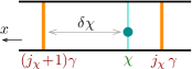
Figure 1: Insertion of a single quasihole at imaginary time $\chi$. The solid vertical lines in orange mark the center positions of the two Landau orbitals sandwiching the quasihole.

We consider a single Abelian quasihole at ${\eta=\chi+i\zeta}$. In Eq. (15), we now have an extra $\hat{\mathcal{Q}}(\chi+i\zeta)$ operator inserted into the chain of electron operators, at the position determined by time ordering. Similar to Eq. (16), we can extract the $\chi$ dependence using the dilation operator,

$$\hat{\mathcal{Q}}(\chi+i\zeta)=e^{\chi\gamma\hat{L}_{0}}\hat{\mathcal{Q}}(i\zeta)e^{-\chi\gamma\hat{L}_{0}}.$$ (31)

Following the same steps from Sec. II.2 to Sec. II.3, for each imaginary-time interval of size $s$ between adjacent primary field (electron or quasihole) insertions, we can capture the dilation and the background charge using the cylinder evolution operator $\hat{U}(s)$ [Eq. (25)].

As a result of the quasihole at $\chi+i\zeta$, the cylinder evolution is now further punctured by $\hat{\mathcal{Q}}(i\zeta)$ at the time slice $\chi$. To locate this time slice relative to the Landau orbitals, recall that the orbital $j$ is centered at $x=\gamma j$ [Eq. (10)]. The $\hat{\mathcal{Q}}(i\zeta)$ operator is thus inserted between the orbitals $j_{\chi}$ and ${j_{\chi}+1}$ (Fig. 1), with

$$j_{\chi}\equiv\left\lfloor{\chi/\gamma}\right\rfloor.$$ (32)

Here, the floor function $\left\lfloor{t}\right\rfloor\in\mathbb{Z}$ denotes the largest integer no greater than $t\in\mathbb{R}$. The insertion of $\hat{\mathcal{Q}}(i\zeta)$ breaks the cylinder evolution $\hat{U}(\gamma)$ associated with the orbital $\hat{C}^{m}$ operator at $j_{\chi}$ into two parts,

$$\hat{U}(\gamma)\,\,\rightarrow\,\,\hat{U}(\delta\chi)\hat{\mathcal{Q}}(i\zeta)\hat{U}(\gamma-\delta\chi),$$ (33)

where $\delta\chi\in(0,\gamma]$ denotes the displacement of $\chi$ from the center of the orbital ${j_{\chi}+1}$ (Fig. 1),

$$\delta\chi\equiv(j_{\chi}+1)\gamma-\chi.$$ (34)

Note that the cylinder evolution operator $\hat{U}(s)$ does not commute with the $\hat{\mathcal{Q}}(i\zeta)$ insertion, and from its definition in term of the path-ordered exponential in Eq. (25), we have

$$\hat{U}(\gamma-\delta\chi)=[\hat{U}(\delta\chi)]^{-1}\,\,\hat{U}(\gamma).$$ (35)

Then, without modifying the $\hat{C}^{m}$ operators, the quasihole $\hat{\mathcal{Q}}(\chi+i\zeta)$ can be represented in Eq. (20) by the insertion of

$$\hat{U}(\delta\chi)\,\hat{\mathcal{Q}}(i\zeta)\,[\hat{U}(\delta\chi)]^{-1}$$ (36)

between the $\hat{C}^{m}$ operators for orbitals $j_{\chi}$ and $j_{\chi}+1$.

There is one extra complication that we have glossed over. When we expand the CFT-derived wave function

$$\Big{\langle}\mathcal{V}(z_{1})\cdots\mathcal{V}(z_{n})\,\mathcal{Q}(\chi+i\zeta)\,\,\mathcal{O}_{\text{bc}}\Big{\rangle}$$ (37)

into Slater-determinant basis states in Eq. (14), we place the electron contours at the center of each occupied orbital. To bring the field insertions into time ordering, the electrons on orbitals with center position $x<\chi$ have to be moved across the pinned quasihole field at time $\chi$. For the Abelian quasihole as in Eq. (30), each of these commutations incurs a minus sign,

$$\langle\cdots\mathcal{V}(z)\mathcal{Q}(\chi+i\zeta)\cdots\rangle=-\,\langle\cdots\mathcal{Q}(\chi+i\zeta)\mathcal{V}(z)\cdots\rangle.$$ (38)

The above anti-commutativity simply reflects the fact that in the planar wave function an Abelian quasihole is represented by the odd-power factor ${\prod_{i}(w_{i}-\eta)}$. Formally, one could also derive this minus sign from the operator product expansion.

We need to collect these minus signs together and attach them to the quasihole insertion. To this end, for each Slater-determinant basis state we have to count the number of occupied orbitals with center position $x<\chi$. This number can be extracted from the conserved U(1) charge at the time slice $\chi$ of the quasihole insertion. [Note that for each orbital the cylinder evolution $\hat{U}(\gamma)$ contained in the $\hat{C}^{m}$ operator correctly accounts for the associated background charge.] Specifically, the number of occupied orbitals with $x<\chi$ is given by

$$\sqrt{\nu}\hat{a}_{0}+(j_{\chi}+1)\nu$$ (39)

inserted between the $\hat{C}^{m}$ operators for orbitals $j_{\chi}$ and $j_{\chi}+1$. Here, the zero-mode $\hat{a}_{0}$ measures the U(1) charge in unit of $\sqrt{\nu}$ times the electron charge $e$, and the second term cancels the background charge $-\nu e$ carried by each orbital $j\in\{0,1,\ldots,j_{\chi}\}$. Finally, we can write down the full expression for the quasihole operator in the MPS

$$\hat{U}(\delta\chi)\,\hat{\mathcal{Q}}(i\zeta)\,[\hat{U}(\delta\chi)]^{-1}\,(-1)^{\sqrt{\nu}\hat{a}_{0}+(j_{\chi}+1)\nu}.$$ (40)

Note that $\hat{a}_{0}$ does not commute with $[\hat{U}(\delta\chi)]^{-1}$, as the latter contains $\hat{\phi}_{0}$.

The above construction can be easily generalized to the case of multiple Abelian quasiholes, with

$$\Big{\langle}\mathcal{V}(z_{1})\cdots\mathcal{V}(z_{n})\,\mathcal{Q}(\chi_{1}+i\zeta_{1})\cdots\mathcal{Q}(\chi_{m}+i\zeta_{m})\,\mathcal{O}_{\text{bc}}\Big{\rangle}.$$ (41)

We put the $m$ quasiholes in time ordering,

$$\chi_{1}>\chi_{2}>\cdots>\chi_{m}.$$ (42)

Then, each quasihole has the MPS representation given by Eq. (40), except for one minor modification. For the ${l\text{-th}}$ quasihole, to extract the number of occupied orbitals with $x<\chi_{l}$, we need to subtract not only the background charge, but also the U(1) charge introduced by the other quasiholes inserted on its right. This modifies the commutation sign in Eq. (40) to

$$(-1)^{\sqrt{\nu}\hat{a}_{0}+(j_{\chi}+1)\nu-(m-l)\nu}.$$ (43)

The last two terms in the exponent [$(j_{\chi}+1)\nu-(m-l)\nu$] only introduce an overall constant phase factor (independent from the electron occupations), but they are necessary to eliminate the branch-cut ambiguity in the fractional power $(-1)^{\sqrt{\nu}\hat{a}_{0}}$. This branch cut ambiguity comes from the fact that the operator $\sqrt{\nu}a_{0}$ now counts fractional quasihole charges.

This finishes our review of the MPS construction in the absence of non-Abelian quasiholes. We conclude this section with a few remarks. First, the quasihole MPS has a rather subtle parametric dependence on the quasihole position $\chi+i\zeta$. This dependence is not holomorphic due to the presence of the nonchiral background charge operator $\mathcal{O}_{\text{bc}}$, and the $\chi$-dependence differs considerably from $\zeta$. The imaginary part $\zeta$ enters the MPS directly (and solely) through the operator insertion $\hat{\mathcal{Q}}(i\zeta)$. The real part $\chi$ controls the location $j_{\chi}$ of this insertion, and thereby affects both the cylinder evolution and the electron-quasihole commutation sign. Second, we note that the amount of U(1) charge carried by an Abelian quasihole operator $\hat{\mathcal{Q}}(i\zeta)$ is exactly opposite to the charge carried by an empty orbital $\hat{C}^{0}=\hat{U}(\gamma)$. This can be seen by comparing the exponents in Eqs. (30) and (25). Therefore, to keep the CFT boundary states fixed, upon inserting a quasihole we need to increase the total number of Landau orbitals by one. Third, in the presence of multiple quasiholes, the conformal correlator exhibits a nontrivial monodromy as a function of quasihole positions. In the MPS, this monodromy manifests itself as branch cuts originating from the center of each quasihole. We will discuss this in details in Sec. III.6. Finally, we emphasize that our prescription for the Abelian quasihole matrix differs from Ref. Zaletel and Mong, 2012 in the more careful handling of the background charge. The new formula here exactly preserves the quasihole-dependent normalization of the conformal correlator. This feature is desirable as it enables us to leverage the plasma analogy when checking the braiding statistics. Wu et al. (2014)

III Non-Abelian Quasiholes

We now proceed to the construction of MPS for the non-Abelian quasiholes. We consider the so-called $(k,r)$-clustered states Bernevig and Haldane (2008) at filling fraction $\nu$ of the lowest Landau level, with $k,r$ being integers and

$$\nu=\frac{k}{k+r}.$$ (44)

The electronic correlations in such states are characterized by the presence of $k$-particle clusters. The fermionic wave function is given by the product of a Jastrow factor and a bosonic part. The latter bosonic wave function vanishes to order $r$ when $(k+1)$ particles come together. The $r=2$ case corresponds to the $\mathbb{Z}_{k}$ Read-Rezayi series, Read and Rezayi (1999) with $k=2$ being the Moore-Read state, Moore and Read (1991) while the $(k,r)=(2,3)$ case is the so-called Gaffnian wave function. Simon et al. (2007) These wave functions can be constructed from chiral conformal correlators of primary fields representing electrons and quasiholes. Read and Rezayi (1999) The electron operator takes the tensor product form

$$\mathcal{V}(z)=\psi(z)\,\otimes:\!e^{i\frac{1}{\sqrt{\nu}}\phi(z)}\!:,$$ (45)

where in addition to the free-boson vertex operator, we also have a primary field $\psi$ in the so-called neutral CFT. The fundamental quasihole is represented by

$$\mathcal{Q}(\eta)=\sigma(\eta)\,\otimes:\!e^{i\frac{\sqrt{\nu}}{k}\phi(\eta)}\!:,$$ (46)

with $\sigma$ being another primary field in the neutral CFT. The reduced exponent in the boson vertex operator reflects the fact that the fundamental quasihole is a further $k$-fold fractionalization of the Abelian quasihole in Eq. (30).

The MPS auxiliary space is now given by the direct product of the truncated Hilbert spaces of the neutral CFT and the free boson. As noted in Sec. II, the free boson Hilbert space can be naturally broken into sectors labeled by the conserved U(1) charge $\hat{a}_{0}$. The neutral CFT Hilbert space can be similarly split into different representations of the neutral Virasoro algebra. Di Francesco et al. (1997) Each representation, called a Verma module, is spanned by the conformal family of Virasoro descendants generated from a single primary state. Therefore, each Verma module of the neutral CFT is labeled by a primary field, which we refer to as the “topological charge” and denote by Latin indices $a,b,c,\ldots$. Taken together, the MPS auxiliary space can be split into different sectors labeled by the topological and the U(1) charges. Estienne et al. (2013b) For later convenience, we define the projector into a single Verma module $c$ as

$$\hat{\mathcal{P}}(c)=\sum_{\alpha\in c}|\alpha\rangle\langle\alpha|.$$ (47)

As shown in Sec. II.5, a quasihole at $\chi+i\zeta$ is represented by the insertion of $\hat{\mathcal{Q}}(i\zeta)$ into the cylinder evolution at time slice $\chi$, as in Eq. (36). There are two extra complications for the non-Abelian case in Eq. (46). First, we need to resolve the topologically degenerate states associated with multiple pinned non-Abelian quasiholes. Second, we need to generalize the anti-commutativity between electrons and Abelian quasiholes in Eq. (38). As noted earlier, a non-Abelian quasihole can be seen as a further $k$-fold fractionalization of an Abelian quasihole. This hints at a $k$-way split of the anti-commutation minus sign. However, to have a single-valued electron wave function, the commutation phase between an electron and a quasihole must square to unity. As we demonstrate below, the solution to this conundrum turns out to be letting each of the $k$ parts of a quasihole anticommute with only one out of every $k$ electrons.

III.1 Neutral CFT examples

Before diving into the details of the quasihole operator, we first go through the field content and the fusion rules of the neutral CFT for a few representative theories. Estienne et al. (2013a, b)

Moore-Read. The neutral CFT for the Moore-Read Pfaffian state Moore and Read (1991) is the minimal model $\mathcal{M}(3,4)$ with central charge $c=\frac{1}{2}$. The primary fields $(\mathbbm{1},\psi,\sigma)$ have scaling dimensions $(0,\frac{1}{2},\frac{1}{16})$. The fusion rules are given by

$$\psi\times\psi =\mathbbm{1}, \sigma\times\psi =\sigma, \sigma\times\sigma =\mathbbm{1}+\psi.$$ (48)

Gaffnian. The neutral CFT for the Gaffnian wave function Simon et al. (2007) is the nonunitary minimal model $\mathcal{M}(3,5)$, with a negative central charge $c=-\frac{3}{5}$. The primary fields $(\mathbbm{1},\psi,\sigma,\varphi)$ have scaling dimensions $(0,\frac{3}{4},-\frac{1}{20},\frac{1}{5})$. The fusion rules involving $\psi$ or $\sigma$ are given by

$$\psi\times\psi =\mathbbm{1}, \psi\times\sigma =\varphi, \psi\times\varphi =\sigma,$$ (49)

$$\sigma\times\sigma =\mathbbm{1}+\varphi, \sigma\times\varphi =\psi+\sigma.$$

$\mathbb{Z}_{3}$ Read-Rezayi. The neutral CFT for the $\mathbb{Z}_{3}$ Read-Rezayi state is the $\mathbb{Z}_{3}$ parafermionic variant Read and Rezayi (1999) of the ${c=\frac{4}{5}}$ minimal model $\mathcal{M}(5,6)$. The Virasoro primary fields $(\mathbbm{1},\psi_{1},\psi_{2},W,\varepsilon,\sigma_{1},\sigma_{2},\varphi)$ have scaling dimensions $(0,\frac{2}{3},\frac{2}{3},3,\frac{2}{5},\frac{1}{15},\frac{1}{15},\frac{7}{5})$ and $\mathbb{Z}_{3}$ charges ${(0,2,1,0,0,1,2,0)}$. This theory actually enjoys an extended $\mathcal{W}_{3}$ algebra Estienne and Santachiara (2009) beyond the Virasoro. In this language, the $W$ field is not a primary field, but rather a descendant of the identity under the larger $\mathcal{W}_{3}$ algebra. Similarly, $\varphi$ is actually a descendant of $\varepsilon$. However, as noted in Ref. Estienne et al., 2013b, the $\mathcal{W}_{3}$ approach is numerically inefficient due to the complexity of the extended algebra and the proliferation of null modes. Hence, in the following we stick to the Virasoro description, but for succinctness we keep $W$ and $\varphi$ implicit whenever possible. With this caveat in mind, the fusion rules involving the electron $\psi\equiv\psi_{1}$ or the quasihole $\sigma\equiv\sigma_{1}$ are given by

$$\psi_{1} \psi_{2} \varepsilon \sigma_{1} \sigma_{2} \psi_{1} \psi_{2} \mathbbm{1} \sigma_{2} \varepsilon \sigma_{1} \sigma_{1} \varepsilon \sigma_{2} \psi_{2}+\sigma_{1} \psi_{1}+\sigma_{2} \mathbbm{1}+\varepsilon$$

Note that the $\sigma\times\sigma$ fusion has multiple outcomes in all of the examples above. Such fusion ambiguity is characteristic of the CFT representation of the non-Abelian quasiholes. For completeness, we list the structure constants for the so-called operator product expansion needed to construct the MPS matrix elements in Appendix C.

III.2 Conformal blocks and fusion trees

We consider conformal correlators with multiple non-Abelian quasihole insertions

$$\Big{\langle}\mathcal{V}(z_{1})\cdots\mathcal{V}(z_{n})\,\mathcal{Q}(\eta_{1})\cdots\mathcal{Q}(\eta_{m})\,\,\mathcal{O}_{\text{bc}}\Big{\rangle}.$$ (50)

Due to the nontrivial fusion rule of the $\sigma$ field in $\mathcal{Q}(\eta)$ [Eq. (46)], for each set of quasihole coordinates, the above expression does not produce a single wave function. Instead, it defines a vector space of degenerate wave functions. Moore and Read (1991) A set of basis states in this space, called conformal blocks, can be obtained by specifying how the fields fuse together in terms of a fusion tree diagram. Moore and Seiberg (1989); Di Francesco et al. (1997) We only need to consider the neutral CFT, since the free boson has trivial fusion rules dictated by the U(1) charge conservation. The structure of the fusion tree reflects the ordering of the successive fusions, and different structures correspond to different basis choices for the same vector space. For a given fusion tree structure, the corresponding conformal-block basis states can be enumerated by finding all the topological charge labelings compatible with the fusion rules.

We now consider the MPS representation of the conformal blocks associated with Eq. (50). This mandates the fields to be fused sequentially in time ordering into the $|\text{in}\rangle$ state. As explained in Sec. II.5, each quasihole is pinned at a particular time slice while the electrons need to be placed at the center of each occupied orbital. This requires us to blend the quasihole operators into the chain of electron operators. Specifically, we have a $\hat{\mathcal{V}}_{0}$ operator placed at the center of each occupied Landau orbital and a $\hat{\mathcal{Q}}(i\zeta)$ operator inserted at each quasihole position $\chi$, and the operators are lined up in time ordering. This leads to a fusion tree with a linear structure. Consider for example the following amplitude for the Moore-Read state

$$\langle\cdots\hat{\mathcal{V}}_{0}\,\hat{\mathcal{Q}}(i\zeta_{1})\,\hat{\mathcal{V}}_{0}\,\hat{\mathcal{Q}}(i\zeta_{2})\,|\mathbbm{1}\rangle.$$ (51)

To reduce clutter, here we have omitted the interleaving cylinder evolution operators $\hat{U}(s)$. The fusion tree takes the form

(52)

where the undecided topological charges $(a,b)$ could be either $(\mathbbm{1},\psi)$ or $(\psi,\mathbbm{1})$ according to the fusion rules. It should be noted that the imaginary time $x$ points in the left direction in the above diagram, in accordance with the operator time ordering. To construct the conformal block for either choice of the topological charges $(a,b)$, we need to materialize the fusion channel choice in Eq. (51). This amounts to inserting a Verma module projector to the left of each field insertion,

$$\langle\cdots\hat{\mathcal{P}}(b)\,\hat{\mathcal{V}}_{0}\,\hat{\mathcal{P}}(a)\,\hat{\mathcal{Q}}(i\zeta_{1})\,\hat{\mathcal{P}}(\sigma)\,\hat{\mathcal{V}}_{0}\,\hat{\mathcal{P}}(\sigma)\,\hat{\mathcal{Q}}(i\zeta_{2})\,|\mathbbm{1}\rangle.$$ (53)

It should be noted that the placement of the electron $\hat{\mathcal{V}}_{0}$ operators depends on how and where the Landau orbitals are occupied. As a result, with quasihole insertions in the bulk, the fusion trees for different Slater-determinant amplitudes naturally have different orderings of their quasihole and electron “branches”. For example, with a non-Abelian quasihole pinned at $\eta=\frac{3}{2}\gamma$, the following two Slater-determinant amplitudes have different operator ordering and thereby different fusion tree structure,

$$\cdots\mathtt{101010}_{\!{}_{\star\!}\!}\mathtt{11} \Rightarrow\quad\langle\cdots \hat{\mathcal{V}}_{0}\hat{\mathcal{V}}_{0}\hat{\mathcal{V}}_{0}\hat{\mathcal{Q}}(0)\hat{\mathcal{V}}_{0}\hat{\mathcal{V}}_{0}|\mathbbm{1}\rangle,$$ (54)

$$\cdots\mathtt{011011}_{\!{}_{\star\!}\!}\mathtt{01} \Rightarrow\quad\langle\cdots \hat{\mathcal{V}}_{0}\hat{\mathcal{V}}_{0}\hat{\mathcal{V}}_{0}\hat{\mathcal{V}}_{0}\hat{\mathcal{Q}}(0)\hat{\mathcal{V}}_{0}|\mathbbm{1}\rangle.$$

Here the occupation numbers are listed in reverse to be consistent with the time ordering, the star marks the position of the quasihole relative to the Landau orbitals, and again we have omitted the interleaving cylinder evolutions in order to highlight the operator ordering. Now, to obtain the correct wave function, we must resolve every Slater-determinant amplitude in the same fusion tree basis. A natural choice is to have all the quasihole fields placed at the beginning (rightmost end) of the linear structure. For the example given above, we want

$$\begin{minipage}[c]{71.13188pt} \includegraphics[width=433.62pt]{fusion_tree_example_reordered.pdf} \end{minipage}.$$ (55)

For each Slater-determinant amplitude, we need to reorganize the time-ordered fusion tree in Eq. (52), by bringing all the quasihole branches across the electrons to the rightmost, while keeping their relative ordering. As we show next, this reshuffling transformation amounts to adding a particular minus sign to each quasihole operator, generalizing the prescription for the Abelian quasihole in Eq. (43).

III.3 Exchanging two branches

To connect the fusion tree with the desired structure in Eq. (55) to the primitive time-ordered tree in Eq. (52), we need to move the quasihole insertions across electron operators into the bulk. The elementary move is

$$\begin{minipage}[c]{42.67912pt} \includegraphics[width=433.62pt]{B_move_left_unlabeled.pdf} \end{minipage}\quad\Rightarrow\quad\begin{minipage}[c]{42.67912pt} \includegraphics[width=433.62pt]{B_move_right_unlabeled.pdf} \end{minipage}.$$ (56)

These two fusion trees span the same vector space, and they can be related by a linear transform

$$\begin{minipage}[c]{42.67912pt} \includegraphics[width=433.62pt]{B_move_left.pdf} \end{minipage}=\sum_{f}\big{[}B^{\sigma\psi c}_{d}\big{]}_{ef}\begin{minipage}[c]{42.67912pt} \includegraphics[width=433.62pt]{B_move_right.pdf} \end{minipage},$$ (57)

which is nothing but the CFT half-braid matrix between the electron and the quasihole fields. It should be noted that the U(1) part of the CFT also contributes a phase factor, even though it has trivial fusions and has been omitted from the above diagrams. Also, for the CFT correlator to represent a physical wave function, the electron operator must be local with respect to the quasiholes. As a result, it does not matter whether the electron-quasihole half braid is done clockwise or counterclockwise. This brings Eq. (57) to a more familiar form,

$$\begin{minipage}[c]{42.67912pt} \includegraphics[width=433.62pt]{B_move_left_twisted.pdf} \end{minipage}=\sum_{f}\big{[}B^{\sigma\psi c}_{d}\big{]}_{ef}\begin{minipage}[c]{42.67912pt} \includegraphics[width=433.62pt]{B_move_right.pdf} \end{minipage}.$$ (58)

Formally, the half-braid matrix $B^{abc}_{d}$ can be decomposed into the so-called $F$ and $R$ moves of the direct-product CFT. Moore and Seiberg (1989) Again, the contribution from the U(1) part must be included despite its omission from the diagrams. The fusion $F$ matrix is a generalization of the Wigner $6j$-symbol,

$$\begin{minipage}[c]{42.67912pt} \includegraphics[width=433.62pt]{F_move_left.pdf} \end{minipage}=\sum_{g}\big{[}F^{abc}_{d}\big{]}_{eg}\begin{minipage}[c]{42.67912pt} \includegraphics[width=433.62pt]{F_move_right.pdf} \end{minipage},$$ (59)

where $g$ is summed over all topological charges compatible with the fusion rules. And the $R$ matrix gives the exchange phase in a definite fusion channel,

$$\begin{minipage}[c]{21.33955pt} \includegraphics[width=433.62pt]{R_move_left.pdf} \end{minipage}=R^{ba}_{g}\begin{minipage}[c]{21.33955pt} \includegraphics[width=433.62pt]{R_move_right.pdf} \end{minipage}.$$ (60)

Note that the fusion tree layout in the above definitions is slightly different from the standard convention in the literature. Kitaev (2006) This is due to our choice of pointing the imaginary time $x$ in the left direction in accordance with the operator time ordering. Composing the $F$ and $R$ moves, we find

$$\begin{minipage}[c]{42.67912pt} \includegraphics[width=433.62pt]{FRF_move_left.pdf} \end{minipage}=\sum_{f,g}\big{[}F^{bac}_{d}\big{]}_{eg}\,R^{ba}_{g}\Big{[}\big{(}F^{abc}_{d}\big{)}^{-1}\Big{]}_{gf}\begin{minipage}[c]{42.67912pt} \includegraphics[width=433.62pt]{FRF_move_right.pdf} \end{minipage}.$$ (61)

The transformation coefficient in the above equation is nothing but $\big{[}B^{abc}_{d}\big{]}_{ef}$. In principle, we can solve the pentagon and the hexagon equations Moore and Seiberg (1989) for the $F$ and the $R$ matrices, and fix the gauge according to the structure constants in the operator product expansion of the chiral fields (see Appendix C). This would be a time-consuming task. In practice, however, we can more easily determine the $B^{\sigma\psi c}_{d}$ matrix from a simple numerical calculation. To this end, we consider the conformal-block version of Eq. (57),

$$\langle d|\,\hat{\mathcal{V}}(iy)\,\hat{\mathcal{P}}(e)\,\hat{\mathcal{Q}}(i\zeta)\,|c\rangle=\\ \sum_{f}\big{[}B^{\sigma\psi c}_{d}\big{]}_{ef}\langle d|\,\hat{\mathcal{Q}}(i\zeta)\,\hat{\mathcal{P}}(f)\,\hat{\mathcal{V}}(iy)\,|c\rangle.$$ (62)

Here, we place the operators at adjacent time slices to avoid complications from the cylinder evolution, and for simplicity we choose the end states $\langle d|$ and $|c\rangle$ to be the primary states in the corresponding Verma modules. Recall that the core part of the MPS implementation is a truncated CFT calculator. By numerically evaluating the two (truncated) correlators in the above equation as functions of $(y,\zeta)$, we can extract the $B^{\sigma\psi c}_{d}$ matrix in the gauge determined by the chiral structure constants.

We first consider the Moore-Read and the Gaffnian states. They are clustered wave functions with ${k=2}$. For these theories, the fusion $\psi\times a$ always yields a unique result for any topological charge $a$. Therefore, the topological charges $d$ and $f$ in Eq. (57) are completely fixed by the choice of $c$ and $e$, namely

$$d =\psi\times e, f =\psi\times c,$$ (63)

with $e$ among the (possibly) multiple fusion outcomes of $\sigma\times c$. This allows us to adopt the shorthand notation

$$\big{[}B^{\sigma\psi c}_{d}\big{]}_{ef}\,\,\rightarrow\,\,\,B^{c}_{e},$$ (64)

and it reduces Eq. (62) to

$$\langle\psi\times e|\,\hat{\mathcal{V}}(iy)\,\hat{\mathcal{P}}(e)\,\hat{\mathcal{Q}}(i\zeta)\,|c\rangle=\\ B^{c}_{e}\,\cdot\,\langle\psi\times e|\,\hat{\mathcal{Q}}(i\zeta)\,\hat{\mathcal{P}}(\psi\times c)\,\hat{\mathcal{V}}(iy)\,|c\rangle.$$ (65)

The single-valuedness of the electron wave function dictates that $B^{c}_{e}$ has to be $\pm 1$. For the Moore-Read state, from the numerics we find

$$B^{\mathbbm{1}}_{\sigma} =B^{\sigma}_{\psi}=1, B^{\psi}_{\sigma} =B^{\sigma}_{\mathbbm{1}}=-1.$$ (66)

And for the Gaffnian state, we have

$$B^{\mathbbm{1}}_{\sigma}=B^{\varphi}_{\psi}=B^{\sigma}_{\varphi}=B^{\varphi}_{\sigma}=1,\quad B^{\sigma}_{\mathbbm{1}}=B^{\psi}_{\varphi}=-1.$$ (67)

Depending on the fusion channel context, the electron and the quasihole fields either commute or anticommute.

For the $\mathbb{Z}_{k=3}$ Read-Rezayi state, due to our choice of keeping the $\mathcal{W}_{3}$ algebra implicit and treating $W$ and $\varphi$ as primary fields, even the electron field $\psi\equiv\psi_{1}$ has nontrivial fusion rules,

$$\psi_{1}\times\psi_{2} =\mathbbm{1}+W, \psi_{1}\times\sigma_{1} =\varepsilon+\varphi,$$ (68)

which would not bode well for our proposed method. However, the implicit $\mathcal{W}_{3}$ symmetry forbids us to split the channels on the right-hand side into separate conformal blocks. To take advantage of this, we bind the Verma module $W$ to $\mathbbm{1}$ and bind $\varphi$ to $\varepsilon$ by redefining the projectors [Eq. (47)],

$$\hat{\mathcal{P}}(\mathbbm{1}) \equiv\sum_{\alpha\in\mathbbm{1},W}|\alpha\rangle\langle\alpha|, \hat{\mathcal{P}}(\varepsilon) \equiv\sum_{\alpha\in\varepsilon,\varphi}|\alpha\rangle\langle\alpha|,$$ (69)

and then we simply forget about $W$ and $\varphi$ when labeling the fusion trees. Now that $W$ and $\varphi$ are formally gone, we are allowed to use the shorthand notation in Eq. (64). Crucially, we verify from the numerics that after such patching (but not before), the reduced linear transform in Eq. (65) still holds. This compatibility can be attributed to the underlying extended $\mathcal{W}_{3}$ algebra. The $B^{c}_{e}$ coefficients are found to be

$$B^{\mathbbm{1}}_{\sigma_{1}} =B^{\psi_{1}}_{\varepsilon}=B^{\varepsilon}_{\psi_{2}}=B^{\sigma_{1}}_{\psi_{1}}=B^{\sigma_{1}}_{\sigma_{2}}=B^{\sigma_{2}}_{\varepsilon}=1,$$ (70)

$$B^{\psi_{2}}_{\sigma_{2}} =B^{\varepsilon}_{\sigma_{1}}=B^{\sigma_{2}}_{\mathbbm{1}}=-1.$$

III.4 Reshuffling quasiholes into the bulk

Through successive applications of the elementary move in Eq. (57), we can achieve the reshuffling

$$\begin{minipage}[c]{71.13188pt} \includegraphics[width=433.62pt]{shuffle_n_left.pdf} \end{minipage}\quad\Rightarrow\quad\begin{minipage}[c]{71.13188pt} \includegraphics[width=433.62pt]{shuffle_n_right_labeled.pdf} \end{minipage}$$ (71)

across an arbitrary number $n$ of electrons. Note that the topological charges at the top and the bottom must agree between the two trees; otherwise the conformal blocks belong to distinct linear spaces. Also, due to the trivial fusion rules of the $\psi$ field in the Moore-Read, the Gaffnian, and the $\mathbb{Z}_{3}$ Read-Rezayi states, all the topological charges are completely fixed by $c$ and $e$. In particular, we deduce that the in-situ fusion channels for the $\sigma$ field after the reshuffling are given by the successive fusion with $n$ $\psi$ fields,

$$e^{\prime} =\psi^{n}\times e, c^{\prime} =\psi^{n}\times c,$$ (72)

and the corresponding projected quasihole operator is

$$\hat{\mathcal{Q}}(e,c,n,i\zeta)\equiv\hat{\mathcal{P}}\big{(}\psi^{n}\times e\big{)}\,\hat{\mathcal{Q}}(i\zeta)\,\,\hat{\mathcal{P}}\big{(}\psi^{n}\times c\big{)}.$$ (73)

The linear transform between the two trees in Eq. (71) consists of a simple sign factor,

$$\begin{minipage}[c]{71.13188pt} \includegraphics[width=433.62pt]{shuffle_n_left.pdf} \end{minipage}=(-1)^{N(e,c,n)}\,\cdot\,\,\begin{minipage}[c]{71.13188pt} \includegraphics[width=433.62pt]{shuffle_n_right.pdf} \end{minipage}.$$ (74)

Here, only a subset of the $n$ $\psi$ fields anticommute with $\sigma$, and

$$N(e,c,n)\in\mathbb{Z}$$ (75)

counts the size of this anticommuting subset. Consider $(e,c,n)=(\sigma,\mathbbm{1},4)$ for the Moore-Read state as an example. Recall from Eq. (66) that $B^{\mathbbm{1}}_{\sigma}=1$ and $B^{\psi}_{\sigma}=-1$. Using Eq. (57), we find

$$=B^{\mathbbm{1}}_{\sigma}\begin{minipage}[c]{82.51282pt} \includegraphics[width=433.62pt]{shuffle_mr_example_2.pdf} \end{minipage}$$ (76)

$$=B^{\mathbbm{1}}_{\sigma}B^{\psi}_{\sigma}\begin{minipage}[c]{82.51282pt} \includegraphics[width=433.62pt]{shuffle_mr_example_3.pdf} \end{minipage}$$

$$=B^{\mathbbm{1}}_{\sigma}B^{\psi}_{\sigma}B^{\mathbbm{1}}_{\sigma}B^{\psi}_{\sigma}\begin{minipage}[c]{82.51282pt} \includegraphics[width=433.62pt]{shuffle_mr_example_4.pdf} \end{minipage}.$$

In the above commuting process, the $\sigma$ field picks up a minus sign $B^{\psi}_{\sigma}=-1$ from only every other $\psi$ field (dashed line). This is a direct consequence of Eq. (66). The alternating pattern in the chain of $\psi$ fields has periodicity two, as expected from the fusion rule $\psi^{2}=\mathbbm{1}$.

Following the above procedure, for each channel choice $(e,c)$, we can identify the subset of $\psi$ fields that anticommute with $\sigma$ (dashed lines). For the Moore-Read state we find,

$$\begin{minipage}[c]{91.04872pt} \includegraphics[width=433.62pt]{shuffle_mr_1.pdf} \end{minipage}, \begin{minipage}[c]{91.04872pt} \includegraphics[width=433.62pt]{shuffle_mr_2.pdf} \end{minipage},$$ (77)

$$\begin{minipage}[c]{91.04872pt} \includegraphics[width=433.62pt]{shuffle_mr_3.pdf} \end{minipage}, \begin{minipage}[c]{91.04872pt} \includegraphics[width=433.62pt]{shuffle_mr_4.pdf} \end{minipage}.$$

Counting the dashed lines, we have for Eq. (74)

$$N(\sigma,\mathbbm{1},n) =N(\psi,\sigma,n)=\left\lfloor{\textstyle\frac{n}{2}}\right\rfloor,$$ (78)

$$N(\sigma,\psi,n) =N(\mathbbm{1},\sigma,n)=\left\lfloor{\textstyle\frac{n+1}{2}}\right\rfloor,$$

where the floor function $\left\lfloor{t}\right\rfloor\in\mathbb{Z}$ denotes the largest integer no greater than $t\in\mathbb{R}$. Similarly, for the Gaffnian state we have

$$\begin{minipage}[c]{91.04872pt} \includegraphics[width=433.62pt]{shuffle_gf_1.pdf} \end{minipage}, \begin{minipage}[c]{91.04872pt} \includegraphics[width=433.62pt]{shuffle_gf_2.pdf} \end{minipage},$$ (79)

$$\begin{minipage}[c]{91.04872pt} \includegraphics[width=433.62pt]{shuffle_gf_3.pdf} \end{minipage}, \begin{minipage}[c]{91.04872pt} \includegraphics[width=433.62pt]{shuffle_gf_4.pdf} \end{minipage},$$

$$\begin{minipage}[c]{91.04872pt} \includegraphics[width=433.62pt]{shuffle_gf_5.pdf} \end{minipage}, \begin{minipage}[c]{91.04872pt} \includegraphics[width=433.62pt]{shuffle_gf_6.pdf} \end{minipage}.$$

And the number of anticommuting $\psi$ fields is given by

$$N(\sigma,\mathbbm{1},n) =N(\psi,\varphi,n) =\left\lfloor{\textstyle\frac{n}{2}}\right\rfloor,$$ (80)

$$N(\varphi,\psi,n) =N(\mathbbm{1},\sigma,n) =\left\lfloor{\textstyle\frac{n+1}{2}}\right\rfloor,$$

$$N(\varphi,\sigma,n) =N(\sigma,\varphi,n) =0.$$

Note that for $(e,c)=(\varphi,\sigma)$ and $(\sigma,\varphi)$, the $\sigma$ field commute with all $\psi$ fields without any minus sign. For the $\mathbb{Z}_{3}$ Read-Rezayi state we find,

$$\begin{minipage}[c]{113.81102pt} \includegraphics[width=433.62pt]{shuffle_rr_1.pdf} \end{minipage},\,\,\bigg{[}\!\begin{array}[]{c}c\\ e\end{array}\!\bigg{]}=\bigg{[}\!\begin{array}[]{c}\mathbbm{1}\\ \sigma_{1}\end{array}\!\bigg{]},\bigg{[}\!\begin{array}[]{c}\sigma_{1}\\ \psi_{1}\end{array}\!\bigg{]},\bigg{[}\!\begin{array}[]{c}\sigma_{2}\\ \varepsilon\end{array}\!\bigg{]};$$ (81)

$$\begin{minipage}[c]{113.81102pt} \includegraphics[width=433.62pt]{shuffle_rr_2.pdf} \end{minipage},\,\,\bigg{[}\!\begin{array}[]{c}c\\ e\end{array}\!\bigg{]}=\bigg{[}\!\begin{array}[]{c}\psi_{1}\\ \varepsilon\end{array}\!\bigg{]},\bigg{[}\!\begin{array}[]{c}\varepsilon\\ \psi_{2}\end{array}\!\bigg{]},\bigg{[}\!\begin{array}[]{c}\sigma_{1}\\ \sigma_{2}\end{array}\!\bigg{]};$$

$$\begin{minipage}[c]{113.81102pt} \includegraphics[width=433.62pt]{shuffle_rr_3.pdf} \end{minipage},\,\,\bigg{[}\!\begin{array}[]{c}c\\ e\end{array}\!\bigg{]}=\bigg{[}\!\begin{array}[]{c}\psi_{2}\\ \sigma_{2}\end{array}\!\bigg{]},\bigg{[}\!\begin{array}[]{c}\sigma_{2}\\ \mathbbm{1}\end{array}\!\bigg{]},\bigg{[}\!\begin{array}[]{c}\varepsilon\\ \sigma_{1}\end{array}\!\bigg{]}.$$

And the number of anti-commuting $\psi_{1}$ fields is given by

$$\!\!\begin{aligned} &N(\sigma_{1},\mathbbm{1},n)=N(\psi_{1},\sigma_{1},n)=N(\varepsilon,\sigma_{2},n)&&=\left\lfloor{\textstyle\frac{n}{3}}\right\rfloor,\\ &N(\varepsilon,\psi_{1},n)=N(\psi_{2},\varepsilon,n)=N(\sigma_{2},\sigma_{1},n)&&=\left\lfloor{\textstyle\frac{n+1}{3}}\right\rfloor,\\ &N(\sigma_{2},\psi_{2},n)=N(\mathbbm{1},\sigma_{2},n)=N(\sigma_{1},\varepsilon,n)&&=\left\lfloor{\textstyle\frac{n+2}{3}}\right\rfloor.\end{aligned}$$ (82)

Again, we emphasize that the sign structure has contributions from both the neutral and the implicit U(1) parts of the direct-product CFT.

III.5 Putting the pieces together

We apply the reshuffling formula (74) to bring the quasihole and the electron fields into time ordering. A quasihole at position $\chi+i\zeta$ should be placed between the orbitals $j_{\chi}\equiv\left\lfloor{\chi/\gamma}\right\rfloor$ and $j_{\chi}+1$ [Eq. (32)]. Starting from the rightmost end of the fusion tree, to reach this time-ordered position, the number of electrons it needs to cross is given by the number of occupied orbitals with center $x<\chi$. Consider $m$ fundamental quasiholes with ordering $\chi_{1}>\cdots>\chi_{m}$ [Eq. (41)]. The number of occupied orbitals with center $x<\chi_{l}$ is counted by the operator

$$\hat{n}_{l}=\sqrt{\nu}\hat{a}_{0}+(j_{\chi_{l}}+1)\nu-\frac{m-l}{k}\nu$$ (83)

inserted between the $\hat{C}^{m}$ operators for orbitals $j_{\chi}$ and $j_{\chi}+1$. The above formula is adapted from the Abelian case [Eq. (43)]. The extra $k$ in the denominator of the last term reflects the further $k$-fold fractionalization of the U(1) charge of a fundamental quasihole in the non-Abelian states [Eq. (46)].

Now we are finally ready to synthesize the full expression for the non-Abelian quasihole operator. We would like to obtain the MPS description of the conformal block with $m$ fundamental quasiholes specified by the fusion tree

$$\begin{minipage}[c]{99.58464pt} \includegraphics[width=433.62pt]{fusion_tree_m.pdf} \end{minipage}.$$ (84)

Here the quasihole fields are placed at the rightmost end of the linear tree structure as in Eq. (55), and we have omitted the electron branches on the left side. The topological charges satisfy $b_{l-1}\in\sigma\times b_{l}$, with $b_{m}=\mathbbm{1}$. In the MPS, the quasiholes are placed in time ordering, and the ${l\text{-th}}$ quasihole with fusion context $(b_{l-1},b_{l})$ is represented by the insertion of

$$\hat{U}(\delta\chi_{l})\,\hat{\mathcal{Q}}(b_{l-1},b_{l},\hat{n}_{l},i\zeta_{l})\,[\hat{U}(\delta\chi_{l})]^{-1}\,(-1)^{N(b_{l-1},b_{l},\hat{n}_{l})}$$ (85)

between the $\hat{C}^{m}$ operators for orbitals $j_{\chi_{l}}$ and ${j_{\chi_{l}}+1}$. In the above expression, the displacement $\delta\chi_{l}$ is defined in Eq. (34), the projected quasihole operator $\hat{\mathcal{Q}}(e,c,n,i\zeta)$ is defined in Eq. (73), the occupied orbital counter $\hat{n}_{l}$ is defined in Eq. (83), and the anticommuting subset counter $N(e,c,n)$ defined in Eq. (74) has values given by Eqs. (78), (80), and (82). The above MPS representation preserves the conformal-block normalization for the non-Abelian quasiholes, and it is the main result of this paper.

III.6 Branch cut structure

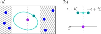
Figure 2: (a) Braiding one quasihole around another. The bystander quasiholes in the shaded regions do not participate in the braiding process other than setting the fusion channel context. The vertical dotted line marks the location of the branch cut discontinuity. (b) An infinitesimal segment of the braiding path crossing the branch cut from above.

As the final note, in this section we examine the monodromy structure of the MPS when we braid one non-Abelian quasihole around another (Fig. 2). The MPS prescription produces conformal blocks in a particular fusion tree basis, where the quasiholes are placed in time ordering at the rightmost end of the linear structure before the electrons. This allows us to focus on the fusion tree segment actively involved in the braiding process

$$\begin{minipage}[c]{71.13188pt} \includegraphics[width=433.62pt]{braiding_tree.pdf} \end{minipage},$$ (86)

without worrying about the bystander quasiholes (Fig. 2) or the electrons, which just define the topological charges $(a,c)$. Due to the time-ordered insertion of the quasiholes, each conformal block develops a branch cut discontinuity when the two quasiholes coincide in the horizontal direction, as illustrated by the dotted lines in Fig. 2(a). This discontinuity represents an abrupt change of basis and does not correspond to a physical singularity. To understand how the conformal blocks across the branch cut are related, we consider the two points infinitesimally close to the cut, as shown in Fig. 2(b). To be specific, we place the stationary quasihole at $\eta_{0}=0$ and examine the infinitesimal segment across the cut above it, from $-\epsilon+i\zeta$ to $\epsilon+i\zeta$. The conformal blocks on the two sides of the cut are given by

$$\begin{minipage}[c]{71.13188pt} \includegraphics[width=433.62pt]{braiding_tree_left.pdf} \end{minipage}\quad\text{and}\quad\begin{minipage}[c]{71.13188pt} \includegraphics[width=433.62pt]{braiding_tree_right.pdf} \end{minipage}.$$ (87)

In the limit of $\epsilon\rightarrow 0^{+}$, the conformal blocks on the right side can be related via continuity to the twisted trees

$$\begin{minipage}[c]{71.13188pt} \includegraphics[width=433.62pt]{braiding_tree_right.pdf} \end{minipage}=\begin{minipage}[c]{71.13188pt} \includegraphics[width=433.62pt]{braiding_tree_right_twisted.pdf} \end{minipage}.$$ (88)

Further, we can untwist the fusion trees using the half-braid $B$ matrix of the direct-product CFT [Eq. (58)],

$$\begin{minipage}[c]{71.13188pt} \includegraphics[width=433.62pt]{braiding_tree_right_twisted.pdf} \end{minipage}=\sum_{d}\big{[}B^{\sigma\sigma a}_{c}\big{]}_{bd}\begin{minipage}[c]{71.13188pt} \includegraphics[width=433.62pt]{braiding_tree_left_d.pdf} \end{minipage},$$ (89)

leading to

$$\begin{minipage}[c]{71.13188pt} \includegraphics[width=433.62pt]{braiding_tree_right.pdf} \end{minipage}=\sum_{d}\big{[}B^{\sigma\sigma a}_{c}\big{]}_{bd}\begin{minipage}[c]{71.13188pt} \includegraphics[width=433.62pt]{braiding_tree_left_d.pdf} \end{minipage}.$$ (90)

Similarly, across the branch cut below the stationary quasihole we find

$$\begin{minipage}[c]{71.13188pt} \includegraphics[width=433.62pt]{braiding_tree_below_left.pdf} \end{minipage}=\sum_{d}\big{[}B^{\sigma\sigma a}_{c}\big{]}_{bd}\begin{minipage}[c]{71.13188pt} \includegraphics[width=433.62pt]{braiding_tree_below_right.pdf} \end{minipage}.$$ (91)

Therefore, the MPS conformal blocks across the branch cuts are related by the half-braid $B$ matrices of the direct-product CFT. In other words, the full-braid monodromy of the conformal blocks are concentrated in the branch cut singularities. This is a special feature of our fusion tree basis with time ordering, and it drastically simplifies the microscopic demonstration of the topological nature of the quasihole braiding statistics. Wu et al. (2014) With the branch cuts contributing the CFT monodromy matrix, now we just need to show that the braiding process away from the branch cuts accumulates only a simple Aharonov-Bohm phase. For the quasihole wave functions constructed from the conformal correlators, the latter condition can be further reduced to the exponential convergence of the overlap matrix between different conformal blocks at large quasihole separations. Bonderson et al. (2011) In an earlier paper, we took advantage of this line of simplifications to demonstrate the Fibonacci nature of the $\mathbb{Z}_{3}$ Read-Rezayi quasiholes. This exploitation depends crucially on the fact that our MPS construction is a literal transcription of the conformal blocks preserving both the monodromy structure and the plasma normalization.

IV Conclusion

In this paper we have presented a pedagogical derivation of the conformal-block MPS for non-Abelian quasiholes. The procedure is exemplified using the Moore-Read, the Gaffnian, and the $\mathbb{Z}_{3}$ Read-Rezayi states. Our prescription preserves the monodromy structure and the plasma normalization of the conformal blocks, and the resulting MPS explicitly manifests the putative quasihole braiding statistics as half-monodromy matrices across branch cuts.

We thank P. Bonderson, V. Mikhaylov, Y. Shen, and M. Zaletel for useful discussions. BAB, NR, and YLW were supported by NSF CAREER DMR-0952428, NSF-MRSEC DMR-0819860, ONR-N00014-11-1-0635, MURI-130-6082, Packard Foundation, and a Keck grant. NR was also supported by the Princeton Global Scholarship. YLW was also supported by LPS-CMTC and JQI-PFC during the final stage of this work.

Appendix A Uniform background charge

In this Appendix we prove Eq. (12), namely that the inclusion of the uniform background charge [Eq. (11)]

$$\mathcal{O}_{\text{bc}}=\,\,:\!\exp\left(-i\frac{\sqrt{\nu}}{2\pi}\int\mathrm{d}^{2}w\,\,\phi(w)\right)\!:$$ (92)

in the conformal correlator correctly produces the Landau-gauge Gaussian factor with an extra non-holomorphic gauge transform, such that

$$\Psi(z_{1},\ldots,z_{n})=e^{i\sum_{i}x_{i}y_{i}}\Big{\langle}\mathcal{V}(z_{1})\cdots\mathcal{V}(z_{n})\,\,\mathcal{O}_{\text{bc}}\Big{\rangle}$$ (93)

is a legitimate many-body wave function in the lowest Landau level with the Landau gauge.

The above statement applies to quantum Hall states described by a generic direct-product CFT. Without loss of generality, we can focus on the U(1) part of the electron operator, ${\mathcal{V}(z)=\,:\!e^{i\frac{1}{\sqrt{\nu}}\phi(z)}\!:}$, since the background charge $\mathcal{O}_{\text{bc}}$ does not couple to the neutral CFT. Further, due to the noninteracting nature of the U(1) boson, we only need to consider the contraction of a single electron operator with the background charge,

$$e^{f(x,y)} \equiv\Big{\langle}\,\,:\!e^{i\frac{1}{\sqrt{\nu}}\phi(x+iy)}\!:\,\,\,:\!e^{-i\frac{\sqrt{\nu}}{2\pi}\int\mathrm{d}x^{\prime}\mathrm{d}y^{\prime}\,\phi(x^{\prime}+iy^{\prime})}\!:\,\,\Big{\rangle}$$ (94)

$$=\exp\left(\frac{1}{2\pi}\int\mathrm{d}x^{\prime}\mathrm{d}y^{\prime}\,\,\langle\phi(x+iy)\phi(x^{\prime}+iy^{\prime})\rangle\right).$$

We work on the cylinder geometry with perimeter $L_{y}$ and inverse radius $\gamma=2\pi/L_{y}$. Plugging the boson propagator

$$\Big{\langle}\phi(z)\phi(0)\Big{\rangle}=-\log\left(\frac{2}{\gamma}\sinh\frac{\gamma z}{2}\right)$$ (95)

into Eq. (94), we find

$$f(x,y)=\\ -\frac{1}{2\pi}\int\mathrm{d}x^{\prime}\mathrm{d}y^{\prime}\log\Bigg{(}\frac{2}{\gamma}\sinh\frac{\gamma\,(x+iy-x^{\prime}-iy^{\prime})}{2}\Bigg{)}.$$ (96)

The integration in the above equation is performed over the cylinder surface $(x^{\prime},y^{\prime})\in\,{\mathbb{R}\times(-\frac{1}{2}L_{y},\frac{1}{2}L_{y})}$. We proceed by separating the real and the imaginary parts of the complex logarithm, $\log u=\log|u|+i\text{Im}\log u$.

The real part of the logarithm is nothing but the Coulomb potential on the cylinder geometry, Aizenman et al. (2010) in the sense that

$$\nabla^{2}\log\left|\frac{2}{\gamma}\sinh\frac{\gamma(z-z^{\prime})}{2}\right|=2\pi\,\delta(z-z^{\prime}),$$ (97)

with cylinder identification $z\sim z+iL_{y}$. The real part of $f(x,y)$ is thus the scalar potential due to the uniform background charge, satisfying

$$\nabla^{2}\text{Re}f(x,y)=-\int\mathrm{d}x^{\prime}\mathrm{d}y^{\prime}\,\delta(x-x^{\prime})\delta(y-y^{\prime})=-1.$$ (98)

Imposing the reflection and the rotational symmetries on the cylinder,

$$\text{Re}f(x,y) =\text{Re}f(-x,y), \partial_{y}\text{Re}f(x,y) =0,$$ (99)

we can integrate the above Poisson equation and obtain

$$\text{Re}f(x,y)=-\frac{x^{2}}{2}.$$ (100)

As claimed, this correctly reproduces the Gaussian factor in the one-body Landau orbital [Eq. (10)].

For the imaginary part of the logarithm, we employ the identity Ogawa (2009)

$$\text{Im}\log\sinh\frac{\gamma\,(x+iy)}{2}=\sum_{n}^{\mathbb{Z}}\arctan\frac{y+nL_{y}}{x}.$$ (101)

It is not hard to see why this holds: starting from $\text{Im}\log\frac{\gamma}{2}(x+iy)=\arctan\frac{y}{x}$, the periodic structure introduced by the hyperbolic sine is matched by the periodic sum over $n$. As a result, the imaginary part of $f(x,y)$ is given by

$$\text{Im}f(x,y) =-\frac{1}{2\pi}\int_{\text{cyl}}\mathrm{d}x^{\prime}\mathrm{d}y^{\prime}\sum_{n}^{\mathbb{Z}}\arctan\frac{y-y^{\prime}+nL_{y}}{x-x^{\prime}}$$ (102)

$$=-\frac{1}{2\pi}\int_{\mathbb{R}}\mathrm{d}x^{\prime}\int_{\mathbb{R}}\mathrm{d}y^{\prime}\arctan\frac{y-y^{\prime}}{x-x^{\prime}}$$

$$=-\frac{y}{2}\int_{\mathbb{R}}\mathrm{d}x^{\prime}\,\text{sign}(x-x^{\prime})=-xy.$$

Here, we have joined the cylinder integrals in the infinite sum to tile the $\mathbb{R}\times\mathbb{R}$ plane, with a symmetric regularization for the $\pm\infty$ limits.

To sum up, we have shown that the contraction with the cylinder background charge is given by

$$\Big{\langle}:\!e^{i\frac{1}{\sqrt{\nu}}\phi(x+iy)}\!:\,\,\,:\!e^{-i\frac{\sqrt{\nu}}{2\pi}\int\mathrm{d}x^{\prime}\mathrm{d}y^{\prime}\,\phi(x^{\prime}+iy^{\prime})}\!:\Big{\rangle}\\ =e^{-ixy}e^{-x^{2}/2}.$$ (103)

This proves that the wave function defined in Eq. (12) indeed lives in the Landau gauge with the correct Gaussian factor.

Appendix B Calculating matrix elements

In the main text the MPS is described in terms of operators acting on the CFT Hilbert space. In this Appendix, we briefly describe the construction of the matrix representation of these operators. A detailed procedure for the calculation of the primary field matrix elements has been published in Ref. Estienne et al., 2013b. Leveraging this result, all we need here is to map the operators of interest from the cylinder geometry to the plane.

Under the conformal map $z\rightarrow e^{\gamma z}$ from the cylinder to the plane, a primary field $\Phi$ with scaling dimension $\Delta_{\Phi}$ transforms by

$$\hat{\Phi}(z)=\left(\gamma e^{\gamma z}\right)^{\Delta_{\Phi}}\,\hat{\Phi}_{\text{plane}}\!\left(e^{\gamma z}\right).$$ (104)

Between two generic CFT energy eigenstates $|\alpha\rangle$ and $|\beta\rangle$ with $\hat{L}_{0}$ eigenvalues $\Delta_{\alpha}$ and $\Delta_{\beta}$, the matrix element of $\hat{\Phi}(iy)$ reads

$$\langle\alpha|\hat{\Phi}(iy)|\beta\rangle =\langle\alpha|e^{iy\gamma\hat{L}_{0}}\hat{\Phi}(0)e^{-iy\gamma\hat{L}_{0}}|\beta\rangle$$ (105)

$$=e^{iy\gamma(\Delta_{\alpha}-\Delta_{\beta})}\gamma^{\Delta_{\Phi}}\langle\alpha|\hat{\Phi}_{\text{plane}}(1)|\beta\rangle.$$

The planar matrix element $\langle\alpha|\hat{\Phi}_{\text{plane}}(1)|\beta\rangle$ can be further related through algebraic manipulations Estienne et al. (2013b) to the structure constant associated with the $\Phi_{\alpha}$ terms in the operator product expansion $\Phi\times\Phi_{\beta}$, where $\Phi_{\alpha}$ and $\Phi_{\beta}$ are the parent primary fields for the states $|\alpha\rangle$ and $|\beta\rangle$. This procedure can be directly applied to the quasihole $\hat{\mathcal{Q}}(i\zeta)$. As for the electron operator, we can reduce the zero mode $\hat{\mathcal{V}}_{0}$ [Eq. (17)] to a similar form,

$$\langle\alpha|\hat{\mathcal{V}}_{0}|\beta\rangle =\gamma^{\Delta_{\mathcal{V}}}\int_{0}^{L_{y}}\frac{\mathrm{d}y}{L_{y}}\,e^{iy\gamma(\Delta_{\alpha}-\Delta_{\beta})}\langle\alpha|\hat{\mathcal{V}}_{\text{plane}}(1)|\beta\rangle$$ (106)

$$=\gamma^{\Delta}\delta_{\Delta_{\alpha},\Delta_{\beta}}\langle\alpha|\hat{\mathcal{V}}_{\text{plane}}(1)|\beta\rangle.$$

The relevant structure constants of the neutral CFT for various quantum Hall states are documented in the next appendix.

As noted in Sec. II.4, on a cylinder with finite perimeter $L_{y}=2\pi/\gamma$ the evolution factor $e^{-\gamma^{2}\hat{L}_{0}}$ allows us to truncate the conformal Hilbert space according to $\hat{L}_{0}$ eigenvalues. In the actual calculations behind our previous paper, Wu et al. (2014) we kept the descendant states with $\hat{L}_{0}<14$ for the Moore-Read and the Gaffnian states, and $\hat{L}_{0}<13$ for the $\mathbb{Z}_{3}$ Read-Rezayi state. This is necessary to reach convergence for cylinder perimeter $L_{y}$ up to $25$ magnetic lengths. The resulting MPS auxiliary space has size up to $3\times 10^{4}$. The calculation of physical observables is carried out over the direct product of two copies of the auxiliary space, one for $\langle\!\langle\Psi|$ and one for $|\Psi\rangle\!\rangle$. The size of this direct-product space can be close to $10^{9}$.

Appendix C Operator product expansions

In the main text we have listed the field content and the fusion rules for the Moore-Read state, the $\mathbb{Z}_{3}$ Read-Rezayi state, and the Gaffnian wave function. To actually construct the MPS matrices, we also need the full operator product expansion with structure constants as noted in the previous appendix. In the following, we use a shorthand notation

$$\Phi_{m}\times\Phi_{n}=\sum_{l}C^{l}_{mn}\Phi_{l}$$ (107)

for the operator product expansion

$$\Phi_{m}(z)\Phi_{n}(0)=\sum_{l}C^{l}_{mn}\,z^{h_{l}-h_{m}-h_{n}}[\Phi_{l}(0)+O(z)],$$ (108)

where $h_{i}$ is the scaling dimension of the primary field $\Phi_{i}$. For the Moore-Read state, we have

$$\psi\times\psi =\mathbbm{1}, \sigma\times\psi =\!\frac{1}{\sqrt{2}}\,\sigma, \sigma\times\sigma =\mathbbm{1}+\!\frac{1}{\sqrt{2}}\,\psi.$$ (109)

For the Gaffnian state, we have

$$\psi\times\psi =\mathbbm{1},\quad\psi\times\sigma=\frac{1}{\sqrt{2}}\,\varphi,\quad\psi\times\varphi=\frac{1}{\sqrt{2}}\,\sigma,$$ (110)

$$\sigma\times\sigma =\mathbbm{1}+C_{1}\,\varphi,\quad\sigma\times\varphi=\frac{1}{\sqrt{2}}\psi+C_{1}\,\sigma,$$

with the constant $C_{1}$ given by

$$C_{1}=e^{i\pi/4}\left({\textstyle\frac{\sqrt{5}-1}{2}}\right)^{1/4}\frac{\Gamma(\frac{4}{5})}{\sqrt{\Gamma(\frac{2}{5})\Gamma(\frac{6}{5})}}.$$ (111)

Finally, for the $\mathbb{Z}_{3}$ Read-Rezayi state, the structure constants are listed in Table 1.

Table 1: The OPE structure constants for the $\mathbb{Z}_{3}$ Read-Rezayi CFT. Listed in column $a$, row $b$ is the fusion result $a\times b$ using the shorthand notation in Eq. (107). The constant $C_{2}$ is given by Ardonne and Schoutens (2007)
$$C_{2}=\frac{1}{2}\sqrt{\frac{\Gamma(\frac{1}{5})}{\Gamma(\frac{4}{5})}\left[\frac{\Gamma(\frac{3}{5})}{\Gamma(\frac{2}{5})}\right]^{3}}.$$

	$\psi_{1}$	$\sigma_{1}$
$\psi_{1}\displaystyle\phantom{\bigg{|}\!\!}$	$\frac{2}{\sqrt{3}}\,\psi_{2}$	$\sqrt{\frac{2}{3}}\,\varepsilon+\frac{1}{3}\sqrt{\frac{7}{2}}\,\varphi$
$\psi_{2}\displaystyle\phantom{\bigg{|}\!\!}$	$\mathbbm{1}-\frac{\sqrt{26}}{9}\,W$	$\frac{1}{\sqrt{3}}\,\sigma_{2}$
$W\displaystyle\phantom{\bigg{|}\!\!}$	$\frac{\sqrt{26}}{9}\,\psi_{1}$	$\frac{1}{9\sqrt{26}}\,\sigma_{1}$
$\varepsilon\displaystyle\phantom{\bigg{|}\!\!}$	$\sqrt{\frac{2}{3}}\,\sigma_{2}$	$\sqrt{\frac{2}{3}}\,\psi_{2}+\sqrt{C_{2}}\,\sigma_{1}$
$\sigma_{1}\displaystyle\phantom{\bigg{|}\!\!}$	$\sqrt{\frac{2}{3}}\,\varepsilon-\frac{1}{3}\sqrt{\frac{7}{2}}\,\varphi$	$\frac{1}{\sqrt{3}}\,\psi_{1}+\sqrt{2C_{2}}\,\sigma_{2}$
$\sigma_{2}\displaystyle\phantom{\bigg{|}\!\!}$	$\frac{1}{\sqrt{3}}\,\sigma_{1}$	$\mathbbm{1}-\frac{1}{9\sqrt{26}}\,W+\sqrt{C_{2}}\,\varepsilon-\sqrt{\frac{C_{2}}{21}}\,\varphi$
$\varphi\displaystyle\phantom{\bigg{|}\!\!}$	$\frac{1}{3}\sqrt{\frac{7}{2}}\,\sigma_{2}$	$-\frac{1}{3}\sqrt{\frac{7}{2}}\,\psi_{2}+\sqrt{\frac{C_{2}}{21}}\,\sigma_{1}$

References

- Tsui et al. (1982) D. C. Tsui, H. L. Stormer, and A. C. Gossard, Phys. Rev. Lett. 48, 1559 (1982).
- Wen (1995) X.-G. Wen, Advances in Physics 44, 405 (1995).
- Laughlin (1983) R. B. Laughlin, Physical Review Letters 50, 1395 (1983).
- Haldane (1983) F. D. M. Haldane, Phys. Rev. Lett. 51, 605 (1983).
- Tserkovnyak and Simon (2003) Y. Tserkovnyak and S. H. Simon, Phys. Rev. Lett. 90, 016802 (2003).
- Prodan and Haldane (2009) E. Prodan and F. D. M. Haldane, Physical Review B 80, 115121 (2009).
- Baraban et al. (2009) M. Baraban, G. Zikos, N. Bonesteel, and S. H. Simon, Phys. Rev. Lett. 103, 076801 (2009).
- Dubail et al. (2012) J. Dubail, N. Read, and E. H. Rezayi, Physical Review B 86, 245310 (2012).
- Zaletel and Mong (2012) M. P. Zaletel and R. S. K. Mong, Physical Review B 86, 245305 (2012).
- Estienne et al. (2013a) B. Estienne, Z. Papic, N. Regnault, and B. A. Bernevig, Physical Review B 87, 161112 (2013a).
- Estienne et al. (2013b) B. Estienne, N. Regnault, and B. A. Bernevig, ArXiv e-prints (2013b), arXiv:1311.2936 [cond-mat.str-el] .
- Wu et al. (2014) Y.-L. Wu, B. Estienne, N. Regnault, and B. A. Bernevig, Phys. Rev. Lett. 113, 116801 (2014).
- Estienne et al. (2015) B. Estienne, N. Regnault, and B. A. Bernevig, Phys. Rev. Lett. 114, 186801 (2015).
- Zaletel et al. (2013) M. P. Zaletel, R. S. K. Mong, and F. Pollmann, Phys. Rev. Lett. 110, 236801 (2013).
- Fannes et al. (1992) M. Fannes, B. Nachtergaele, and R. F. Werner, Communications in Mathematical Physics 144, 443 (1992).
- Schollwöck (2011) U. Schollwöck, Annals of Physics 326, 96 (2011).
- Belavin et al. (1984) A. A. Belavin, A. M. Polyakov, and A. B. Zamolodchikov, Nuclear Physics B 241, 333 (1984).
- Fubini (1991) S. Fubini, Modern Physics Letters A 06, 347 (1991).
- Moore and Read (1991) G. Moore and N. Read, Nuclear Physics B 360, 362 (1991).
- Eisert et al. (2010) J. Eisert, M. Cramer, and M. B. Plenio, Rev. Mod. Phys. 82, 277 (2010).
- Simon et al. (2007) S. H. Simon, E. H. Rezayi, N. R. Cooper, and I. Berdnikov, Physical Review B 75, 075317 (2007).
- Read and Rezayi (1999) N. Read and E. Rezayi, Physical Review B 59, 8084 (1999).
- Kitaev (2003) A. Y. Kitaev, Annals of Physics 303, 2 (2003).
- Nayak et al. (2008) C. Nayak, A. Stern, M. Freedman, and S. Das Sarma, Reviews of Modern Physics 80, 1083 (2008).
- Moore and Seiberg (1989) G. Moore and N. Seiberg, Communications in Mathematical Physics 123, 177 (1989).
- Di Francesco et al. (1997) P. Di Francesco, P. Mathieu, and D. Sénéchal, Conformal Field Theory (Springer-Verlag, New York, 1997).
- Nayak and Wilczek (1996) C. Nayak and F. Wilczek, Nuclear Physics B 479, 529 (1996).
- Ardonne and Schoutens (2007) E. Ardonne and K. Schoutens, Annals of Physics 322, 201 (2007).
- Arovas et al. (1984) D. Arovas, J. R. Schrieffer, and F. Wilczek, Phys. Rev. Lett. 53, 722 (1984).
- Gurarie and Nayak (1997) V. Gurarie and C. Nayak, Nuclear Physics B 506, 685 (1997).
- Read (2009) N. Read, Phys. Rev. B 79, 045308 (2009).
- Bonderson et al. (2011) P. Bonderson, V. Gurarie, and C. Nayak, Physical Review B 83, 075303 (2011).
- Rezayi and Haldane (1994) E. H. Rezayi and F. D. M. Haldane, Phys. Rev. B 50, 17199 (1994).
- Yurov and Zamolodchikov (1990) V. P. Yurov and A. B. Zamolodchikov, International Journal of Modern Physics A 05, 3221 (1990).
- Bernevig and Haldane (2008) B. A. Bernevig and F. D. M. Haldane, Physical Review Letters 100, 246802 (2008).
- Estienne and Santachiara (2009) B. Estienne and R. Santachiara, Journal of Physics A: Mathematical and Theoretical 42, 445209 (2009).
- Kitaev (2006) A. Kitaev, Annals of Physics 321, 2 (2006).
- Aizenman et al. (2010) M. Aizenman, S. Jansen, and P. Jung, Annales Henri Poincaré 11, 1453 (2010).
- Ogawa (2009) H. Ogawa, ArXiv e-prints (2009), arXiv:0903.3789 [cond-mat.soft] .