An index-resolved fixed-point homotopy and potential energy landscapes

Abstract

Stationary points (SPs) of the potential energy landscapes can be classified by their Morse index, i.e., the number of negative eigenvalues of the Hessian evaluated at the SPs. In understanding chemical clusters through their potential energy landscapes, only SPs of a particular Morse index are needed. We propose a modification of the “fixed-point homotopy” method which can be used to directly target stationary points of a specified Morse index. We demonstrate the effectiveness of our approach by applying it to the Lennard-Jones clusters.

I Introduction

The stationary points (SPs) of the potential energy function, $V({\mathbf{x}})$, with ${\mathbf{x}}=(x_{1},\dots,x_{n})$, are the bases of the potential energy landscape methods that have recently gained significant attention from the chemical physics community Wales (2004). Finding SPs of $V({\mathbf{x}})$ amounts to solve the corresponding system of nonlinear equations $\frac{\partial V({\mathbf{x}})}{\partial x_{i}}=0$, $i=1,\dots,N$. The stability and the local geometry of the SPs are determined by the eigenvalues of the Hessian matrix of $V({\mathbf{x}})$, $\mathcal{H}(V)({\mathbf{x}})_{ij}=\partial^{2}V/\partial x_{i}\partial x_{j}$, evaluated at the SPs. While the eigenvalues themselves depend on the choice of coordinate systems, by the Sylvester’s Law of Inertia, their signs are independent from coordinate systems and hence are intrinsic to the local geometry of the SPs. The number of negative eigenvalues of $\mathcal{H}(V)({\mathbf{x}})$ is known as the Morse index or simply index. An SP ${\mathbf{x}}$ is said to be degenerate if $\mathcal{H}(V)({\mathbf{x}})$ is singular and nondegenerate otherwise.

A plenty of numerical methods to solve such systems of nonlinear equations Morgan and Sommese (1987); Nocedal (1980); Liu and Nocedal (1989); Trygubenko and Wales (2004); Wales (1992, 1993); Munro and Wales (1999); Henkelman and Jónsson (1999); Kumeda, Munro, and Wales (2001); Gwaltney et al. (2008); Duncan et al. (2014a); Doye and Wales (2002); Duncan et al. (2014b); Grosan and Abraham (2008); Hughes, Mehta, and Wales (2014); Xiao, Wu, and Henkelman (2014); Henkelman, Jóhannesson, and Jónsson (2002) as well as methods to certify numerical approximations Mehta, Hauenstein, and Wales (2013, 2014) are available in the energy landscape areas and beyond (see Ref. Mehta and Grosan, 2015 for a recent short survey). Among these, homotopy continuation methods have long been used to solve multivariate nonlinear systems of equations (see Ref. Allgower and Georg, 2003 for surveys in this subject). Among a rich body of works applying homotopy methods to scientific problems (e.g. Ref. Lee and Chiang, 2004), recently, the numerical polynomial homotopy continuation method Sommese and Wampler (2005); Mehta (2009, 2011a, 2011b); Kastner and Mehta (2011); Martinez-Pedrera et al. (2013); Mehta, Stariolo, and Kastner (2013); Mehta et al. (2014a) has gained special attention for its ability to find all the complex and real SPs of the potentials with polynomial-like nonlinearities. However, when one is interested in finding only real solutions, this method may turn out to be computationally expensive. The authors have applied another homotopy based method, the Newton homotopy, which can be restricted to find only real solutions, with noteworthy resultsMehta et al. (2014b, ). However, this method, same as almost all homotopy based methods, does not distinguish among SPs of different indices whereas in chemical physics applications, finding stable structures and other thermodynamic properties of the systems utilizes only on SPs of indices zero (called minima) and one (called transition states) Wales (2004).

Among the great variety of homotopy methods, the fixed-point homotopy method Davidenko (1953); Scarf (1967); Kellogg, Li, and Yorke (1976), being one of the first general homotopy methods invented, has long been suspected to be able to target index 0. Allgower and Georg (1979) Modifications to the fixed-point homotopy method have been proposed to target a wider range of SPs, especially index 1 SPs. Most notable among them was the “singular fixed-point homotopy” method Lee and Chiang (2004) which uses index 0 SPs as bifurcated starting points and is likely to be able to reach nearby SPs of index 1.

Several other methods have been developed which attempt to find SPs of specific index. Some of the more direct methods include eigenvector following methods Doye and Wales (2002); Wales and Doye (2003), single- and double-ended searches and gradient square based methods Trygubenko and Wales (2004); Wales (1992, 1993); Munro and Wales (1999); Henkelman and Jónsson (1999); Kumeda, Munro, and Wales (2001); Duncan et al. (2014a); Konda, Avdoshenko, and Makarov (2014), etc. However, most of these methods are only locally convergent, i.e., one needs to start from an initial guess close to the actual SP. Moreover, some of these methods also require at least one SP to start with.

In the present contribution, we propose a novel modification to the fixed-point homotopy which can directly target SPs of a given index. Unlike the “singular fixed-point homotopy” method, our proposed method starts with random starting points and does not require an existing collection of index zero SPs as starting points (cf. Ref. Lee and Chiang, 2004), and it is hence more likely to provide a global sample of index 1 SPs. This feature is of particular importance when no index zero SP is known. Compared to other methods based on gradient flow or quasi-Newton techniques, the proposed method is also likely to have a strong advantage in dealing with degenerate SPs Mehta et al. (2014b, ).

II The deformation of an energy landscape

In the following, $V({\mathbf{x}})$ the potential enrgy function to be explored will be called the target potential energy function. For an integer $m$ with $0\leq m\leq n$, called the target index, our goal is to locate SPs ${\mathbf{x}}=(x_{1},\dots,x_{n})\in\mathbb{R}^{n}$ with index exactly $m$. That is, we would like to find points ${\mathbf{x}}\in\mathbb{R}^{n}$ such that

1. $\nabla V({\mathbf{x}})=\boldsymbol{0}$; and

2. $\mathcal{H}(V)$ at ${\mathbf{x}}$ has $m$ negative eigenvalues.

Criterion 1 amounts to solving a system of nonlinear equations. In the present article, we focus on a homotopy continuation approach for solving this problemAllgower and Georg (1979, 2003); Mehta et al. (2014b, ); Li and Yorke (1979) in which the target potential function $V$ is embedded into a family of closely related potential functions $\hat{V}_{t}$ parametrized by a parameter $t$ so that at $t=1$, $\hat{V}_{1}=V$. Geometrically speaking, this can be understood as the continuous deformation of the target energy landscape among a family of related landscapes. The deformation is constructed so that the SPs of one member $\hat{V}_{0}$ at $t=0$ can be studied easily. The movement of the SPs of $\hat{V}_{0}$ under this deformation as $t$ varies from 0 to 1 can then be tracked. In particular, robust numerical algorithms can be used to trace the trajectory of the SPs. If the trajectory can be extended to $t=1$, an SP of the target potential is then produced as $\hat{V}_{1}\equiv V$.

In certain cases, the index can be preserved along the trajectory formed by the aforementioned deformation. By the continuity of eigenvalues of $\mathcal{H}(\hat{V}_{t})$ along a trajectory it is easy to see that the index must remain the same unless a degenerate SP of $\hat{V}_{t}$ is encountered where at least one eigenvalue of $\mathcal{H}(\hat{V}_{t})$ vanishes. However, this criterion is quite limited, since from the point of view of catastrophe theoryPoston and Stewart (2014); Wales (2001) as one traces the SPs of a family of potential functions, an encounter with a degenerate SP is not only possible, but sometimes necessary.

In the following we propose a new homotopy construction that can potentially target SPs of a given index under much relaxed conditions.

III Index-resolved fixed-point homotopy

The fixed-point homotopy Davidenko (1953); Scarf (1967) is one of the first homotopy methods devised to solve general nonlinear systems. Here we propose an “index-resolved fixed-point homotopy” method for finding SPs of a given index. As we shall demonstrate in §IV with experiments on the Lennard-Jones cluster, it is capable of quickly obtaining a large number of SPs of a given index.

In keeping with the general framework for finding SPs of a smooth potential using homotopy methods described above, we construct a family of closely related potential $\hat{V}_{t}$ parametrized by $t$ so that $\hat{V}_{1}\equiv V$ yet the SPs of the starting potential $\hat{V}_{0}$ can be located and studied easily. Here the starting potential is chosen to be the “standard $m$-saddle” located at a point ${\mathbf{a}}=(a_{1},\ldots,a_{n})$ which is represented by the potential

$$-(x_{1}-a_{1})^{2}-\cdots-(x_{m}-a_{m})^{2}+(x_{m+1}-a_{m+1})^{2}+\cdots+(x_{n}-a_{n})^{2}.$$ (1)

Clearly, ${\mathbf{x}}={\mathbf{a}}$ is a nondegenerate SP of the above function with index exactly $m$. For brevity, we define the quadratic form as

$$J^{(m)}({\mathbf{u}})=\frac{1}{2}\begin{bmatrix}u_{1}&\cdots&u_{n}\end{bmatrix}\begin{bmatrix}-I_{m}&\\ &I_{n-m}\end{bmatrix}\begin{bmatrix}u_{1}\\ \vdots\\ u_{n}\end{bmatrix},$$ (2)

where ${\mathbf{u}}=(u_{1},\ldots,u_{n})$, and $I_{m}$ and $I_{n-m}$ are identity matrices of dimension $m\times m$ and $(n-m)\times(n-m)$, respectively. The standard $m$-saddle (1) at ${\mathbf{x}}={\mathbf{a}}$ is then represented by the quadratic function $J^{(m)}({\mathbf{x}}-{\mathbf{a}})$.

Representing the deformation between this $m$-saddle and the target potential $V$ is the one-parameter family

$$\hat{V}^{(m)}_{t}({\mathbf{x}}):=(1-t)\,J^{(m)}({\mathbf{x}}-{\mathbf{a}})+t\,V({\mathbf{x}}).$$ (3)

This family contains the target potential $V({\mathbf{x}})$ as a member, since at $t=1$, $\hat{V}^{(m)}_{1}\equiv V$. The starting potential $\hat{V}^{(m)}_{0}({\mathbf{x}})\equiv J^{(m)}({\mathbf{x}}-{\mathbf{a}})$, at $t=0$, has a unique SP of index $m$. As $t$ varies, $\hat{V}^{(m)}_{t}$ represents a smooth deformation between the two potentials.

We now consider the effect of the deformation (3) on the SP ${\mathbf{x}}={\mathbf{a}}$, that is, how the SP ${\mathbf{x}}={\mathbf{a}}$ of $\hat{V}^{(m)}_{0}$ relates to SPs of nearby members of $\hat{V}^{(m)}_{t}$ as $t$ moves away from $t=0$. The local theory of smooth real-valued functions yields that under a small perturbation, nondegenerate SPs remain nondegenerate, i.e., by varying $t$ sufficiently close to 0, the nondegenerate SPs of $\hat{V}^{(m)}_{t}$ traces out a small piece of smooth curve. The homotopy continuation approach hinges on the “continuation” of this small piece of curve into a globally defined curve that could potentially connect the SP ${\mathbf{x}}={\mathbf{a}}$ of $\hat{V}^{(m)}_{0}$ to an SP of the target potential $\hat{V}^{(m)}_{1}\equiv V$ which we aim to find. A standard application of the Generalized Sard’s Theorem Abraham and Robbin (1967) guarantees that this is possible for “generic” choices of ${\mathbf{a}}$. Putting aside the technical statement of the theorem, it essentially means that if ${\mathbf{a}}$, the (unique) SP of the starting potential, is chosen at random, then with probability one the set of all SPs of $\hat{V}^{(m)}_{t}$ for $t\in[0,1)$ form of smooth curves in the $(n+1)$-dimensional ${\mathbf{x}}$-$t$ space. Among them, we focus on the curve that passes through ${\mathbf{x}}={\mathbf{a}}$ and $t=0$, which will be called the trajectory of ${\mathbf{a}}$. Since $\hat{V}^{(m)}_{1}\equiv V$, if this trajectory extends to $t=1$ then an SP of the target potential is obtained.

From the algebraic standpoint, if we define the index-resolved fixed-point homotopy with index $m$ as

$$H^{(m)}({\mathbf{x}},t):=\nabla\hat{V}^{m}_{t}({\mathbf{x}}),$$ (4)

then the crux of the method is to numerically trace along the smooth trajectory which is a curve defined by $H^{(m)}({\mathbf{x}},t)=\boldsymbol{0}$ and containing the point $({\mathbf{a}},0)$ in the hope that a point $({\mathbf{x}}^{(1)},1)$ can be reached .

While there is a rich selection of numerical methods for tracing such curves, within the community of homotopy methods, a special class of methods based on a predictor-corrector scheme together with an arc-length parametrization of the curve has emerged as the method of choice for its superior stability and efficiency Mehta et al. (2014b); Allgower and Georg (2003); Chu (1983); Allgower (1981); Li and Yorke (1979); Chu (1984); Sommese and Wampler (2005).

Our goal, however, is to locate SPs of index $m$. Since the starting point ${\mathbf{x}}={\mathbf{a}}$ is an index-$m$ SP of the starting potential $\hat{V}^{(m)}_{0}$, the hope is that this index is inherited by the SP of the target potential the trajectory obtains (if the trajectory reaches $t=1$). Clearly, if the trajectory encounters no degenerate SP, the continuity of eigenvalues of $\mathcal{H}(\hat{V}^{(m)}_{t})$ (which must remain nonzero without encountering a degenerate SP) ensures preservation of index along the entire trajectory, and consequently the SP of the target potential it reaches has index $m$. However, our numerical experiments with the Lennard-Jones potential (§IV) suggest that the index can be preserved even when the assumption in this theorem fails to hold, that is, when the trajectory encounters some turning points. Some observations are presented in §V.

III.1 Summary of the Proposed Numerical Algorithm

For the target potential function $V({\mathbf{x}})$ and a given target index $m\leq n$, one first randomly pick a starting point ${\mathbf{a}}\in\mathbb{R}^{n}$ with which the family

$$\hat{V}^{(m)}_{t}({\mathbf{x}}):=(1-t)\,J_{m}({\mathbf{x}}-{\mathbf{a}})+t\,V({\mathbf{x}})$$

is constructed. We are interested in the SPs of $\hat{V}^{(m)}_{t}$ for all $t$ as a set in the $(n+1)$-dimensional space. This set is defined by the nonlinear system $H^{(m)}({\mathbf{x}},t):=\nabla\hat{V}^{(m)}_{t}=\boldsymbol{0}$. The starting point $({\mathbf{a}},0)$ is clearly in this set. Moreover, for generic choices of ${\mathbf{a}}$, this system defines smooth trajectory with the starting point ${\mathbf{x}}={\mathbf{a}}$ and $t=0$.

One can then apply efficient numerical methods based on the predictor-corrector scheme to trace along the smooth trajectory. If the trajectory extends to $t=1$, i.e., if it passes through a point $({\mathbf{x}},t)=({\mathbf{x}}^{(1)},1)$, then an SP of the target potential function $V$ is produced.

III.2 An example

As an example, consider the potential function

$$V(x,y)=-x^{3}+y^{3}+2xy-6,$$ (5)

whose contour plot is shown in Figure 1. It has two SPs: a local minimum (index 0) at $(-2/3,2/3)$ and a saddle point (index 1) at $(0,0)$.

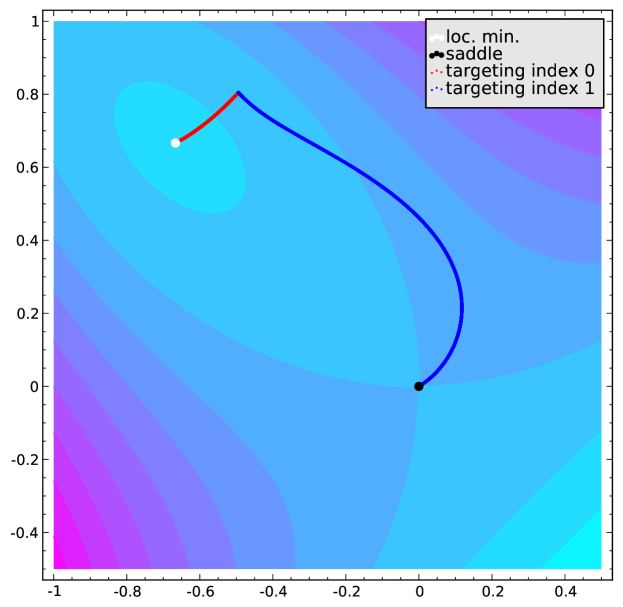
Figure 1: Contour plot of potential function (5) which has a local minimum (index 0) at $(-2/3,2/3)$ and a saddle point (index 1) at $(0,0)$. Starting from the exact same point the two index-resolved fixed-point homotopies with different target indices $\hat{V}^{0}_{t}$ and $\hat{V}^{1}_{t}$ define two different trajectories marked by the red/light and the blue/dark curves respectively.

(Index 0) To locate the index 0 SP we construct

$$\hat{V}^{(0)}_{t}:=\frac{1-t}{2}[(x-a_{1})^{2}+(y-a_{2})^{2}]+t\,V(x,y)$$ (6)

according to (3) with target index $m=0$ where $(a_{1},a_{2})=(-0.494332,0.804689)$ is a randomly chosen starting point. Clearly, $(x,y)=(a_{1},a_{2})$ is an SP of index 0 of the starting potential $\hat{V}^{(0)}_{0}=(x-a_{1})^{2}+(y-a_{2})^{2}$.

The projection of the smooth trajectory, defined by $H^{(0)}(x,y):=\nabla\hat{V}_{t}^{(0)}(x,y)=(0,0)$, onto the $x$-$y$ plane (where $t$ is removed) is shown in Figure 1 as the red/light curve. It converges to the index 0 SP at $(-2/3,2/3)$.

(Index 1) To locate the index 1 SP, we construct

$$\hat{V}^{(1)}_{t}:=\frac{1-t}{2}[-(x-a_{1})^{2}+(y-a_{2})^{2}]+tV(x,y)$$ (7)

with the only difference from (6) being the sign of $(x-a_{1})^{2}$. With the same starting point $(a_{1},a_{2})=(-0.494332,0.804689)$, $H^{(1)}(x,y):=\nabla\hat{V}_{t}^{(1)}(x,y)=(0,0)$ defines a different trajectory whose projection onto the $x$-$y$-plane is shown in Figure 1 as the blue/dark curve. This curve converges to the saddle point $(0,0)$ of $V(x,y)$ instead. It is worth pointing out that even though the starting point $(a_{1},a_{2})$ is very close to the index 0 SP, as shown in Figure 1, the trajectory still converges to the index 1 SP which is much further way.

In both cases, the target indices $m$ in (6) and (7) determine which SP the corresponding curve converge to.

IV The Lennard-Jones Cluster

We apply our method to find SPs of the Lennard-Jones cluster Jones and Ingham (1925) of $N$ atoms whose potential function is given as

$$V_{N}=4\epsilon\sum_{i=1}^{N}\sum_{j=i+1}^{N}\left[\left(\frac{\sigma}{r_{ij}}\right)^{12}-\;\left(\frac{\sigma}{r_{ij}}\right)^{6}\right],$$ (8)

where $N$ is the number of atoms, $2^{1/6}\sigma$ is the equilibrium pair separation, $\epsilon$ is the pair well depth, and

$$r_{ij}=\sqrt{(x_{i}-x_{j})^{2}+(y_{i}-y_{j})^{2}+(z_{i}-z_{j})^{2}}$$

is the Euclidean distance between an $i$-th and $j$-th atoms. We take $\epsilon=\sigma=1$ for simplicity. In addition to the fact that the Lennard-Jones cluster potential serves as a good approximate for the atomic interactions, the potential exhibits complicated landscape structure, i.e., the number of minima exponentially grows when increasing $N$ and has a multi-funnel structure due to the simultaneous presence of competing growth sequences Wales (2004). This model has been under extensive searches for minima and higher index SPs Doye and Wales (2002); Doye and Massen (2005) which provided us bases for comparison.

Defined in terms of the pairwise distances, $V_{N}$ is clearly invariant under rotation and translation. Consequently in the $x$-$y$-$z$ coordinates, all SPs would have certain degrees of freedom. After a translation of the cluster, we can fix the first atom at the origin, i.e., $x_{1}=y_{1}=z_{1}=0$. For the ease of computation, we shall restrict our attention to the cases where the $N$ atoms are not collinear. We can therefore fix $y_{2}=z_{2}=z_{3}=0$ and also require $y_{3}\neq 0$. After the restriction, we have a total of $3N-6$ variables in $V_{N}$. Due to the permutation symmetry, $V_{N}$ may exhibit the same value at different SPs. Such SPs are known as permutation-inversion isomers. Wales (2010); F. Calvo and Wales (2012)

Target	Obtained	$N$
index	index	5	6	7	8	9	10	11	12	13	14	15
$m=0$	0	1 (22)	2 (59)	4 (101)	8 (134)	15 (101)	28 (132)	45 (46)	58 (193)	68 (110)	60 (92)	70 (78)
$m=1$	1	2 (53)	3 (92)	8 (105)	13 (148)	22 (100)	57 (391)	65 (243)	80 (385)	79 (313)	70 (96)	64 (242)
$m=2$	2	4 (44)	6 (168)	8 (142)	14 (170)	14 (96)	15 (106)	56 (124)	52 (143)	57 (119)	55 (115)	52 (97)

Table 1: Numbers of geometric configurations of $N$ atoms (together with numbers of SPs representing them) with different indices of the Lennard-Jones potential $V_{N}$ (8) for a range of $N$ values obtained by index-resolved fixed-point homotopies with target indices $m=0,1,2$ respectively. E.g., the entry “2 (59)” for $N=6$, $m=0$, and “obtained index” 0 indicates that a total of 59 SPs of $V_{6}$ having index 0 are found using the homotopy $H^{(0)}$, and under the permutation symmetry they collectively represent two geometric configurations of the 6 atoms. No nondegenerate SPs of any other indices were found in these runs.

We applied the index-resolved fixed-point homotopy to the problem of finding SPs of the Lennard-Jones potential $V_{N}$ with certain indices. Since SPs of indices 0 (local minima), 1 (transition states), and 2 are most frequently used in computational chemistry, we restrict our attention to homotopies $H^{(m)}$ (as defined in (4)) with $m=0,1,2$, although general constructions with any $m\leq 3N-6$ are possible. Doye and Wales (2002); Doye and Massen (2005) Table 1 shows the number of SPs of $V_{N}$ for a range of $N$ values obtained by $H^{(0)}$, $H^{(1)}$, and $H^{(2)}$ respectively. Remarkably, the indices of all SPs found match exactly the target index $m$ used in the construction of $H^{(m)}$, suggesting that the index-resolved fixed-point homotopy proposed here has a great potential in targeting SPs of a specific index.

As a homotopy-based method, the index-resolved fixed-point homotopy has a strong advantage in dealing with degenerate SPs.Mehta et al. (2014b) The runs that produced SPs listed in Table 1 have also resulted in a number of SPs that appear to be degenerate (and hence not counted). Table 2 lists a selection of these numerically degenerate SPs where Hessian matrices $\mathcal{H}(V_{N})$ have eigenvalues of magnitude less than $10^{-10}$. Though the physical meaning of the degenerate SPs in the Lennard-Jones clusters appear to be understudied, their very presence highlights the richness of the energy landscape and merits further analysis.

$N$	$V_{N}$ at SP	# neg. eig.	# zero eig.	Min. eig.
5	$-3.0000000002858558$	0	6	$10^{-13}$
5	$-4.0000000000004334$	0	5	$10^{-19}$
5	$-6.0000000000157154$	0	3	$10^{-14}$
6	$-6.0000000007539667$	0	6	$10^{-13}$
6	$-8.4806201568350339$	1	3	$10^{-12}$
6	$-9.1038524157210112$	0	3	$10^{-14}$
7	$-9.1038524162043597$	0	6	$10^{-13}$
8	$-12.302927529932436$	0	6	$10^{-13}$
8	$-14.811129645604781$	1	3	$10^{-13}$
8	$-15.444733800924601$	1	3	$10^{-12}$
8	$-15.533060054591045$	0	3	$10^{-15}$
8	$-16.505384168030663$	0	3	$10^{-15}$
9	$-18.597348435556142$	1	3	$10^{-12}$
9	$-18.778208174125020$	0	3	$10^{-14}$
10	$-18.856826168132727$	0	6	$10^{-16}$

Table 2: A selection of numerically degenerate SPs of $V_{N}$ obtained by the index-resolved fixed-point homotopy (4) for a range of $N$ values. For each SP, “$V_{N}$ at the SP” is the value of $V_{N}$ evaluated at the SP. “# neg. eig.” is the number of negative eigenvalues of $\mathcal{H}(V_{N})$ at the SP. “# zero eig.” is the number of eigenvalues of $\mathcal{H}(V_{N})$ at the SP that have magnitude less than $10^{-10}$ and do not correspond to the inherent degree of freedom induced by rotation and translation. “Min. eig.” shows the approximate scale of the of the smallest magnitude of the eigenvalues counted in the column “# zero eig.”.

V Preservation of index under relaxed conditions

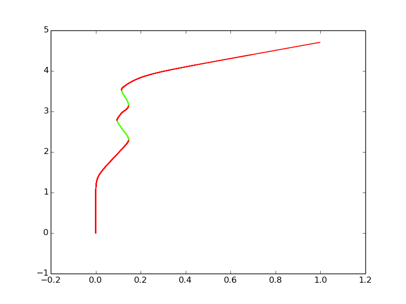
Figure 2: The $t$ value (horizontal) plotted against the arc-length (vertical) along a trajectory of the index-resolved fixed-point homotopy with $N=7$ and $m=2$. For each point $({\mathbf{x}},t)$, the index of ${\mathbf{x}}$ as an SP of $\hat{V}^{(2)}_{t}$ is indicated by color: red/dark for index 2 and green/light for index 1.

As discussed in §II, by the continuity of eigenvalues of $\mathcal{H}(\hat{V}^{(m)}_{t})$ along the trajectory of ${\mathbf{x}}={\mathbf{a}}$, the index must remain the same as long as no degenerate SP of $\hat{V}^{(m)}_{t}$ is encountered (where $\mathcal{H}(\hat{V}^{(m)}_{t})$ becomes singular). However, our numerical experiments with the Lennard-Jones cluster (§IV) suggest that the index can be preserved under much more relaxed conditions. In particular, we observed that index can be preserved even when turning points are encountered. Figure 2 shows the $t$-value plot together with the changes of indices along a curve defined by $H^{(2)}=\boldsymbol{0}$ for the Lennard-Jones cluster potential (8) with $N=7$ and target index $m=2$. After four changes (from index 2 to 1, then 2, 1, and back to 2), the index comes back to the target index $m=2$.

Among our experiments summarized in Table 1, such phenomenon where trajectories encounter some degenerate SPs before reaching SPs of the target potential appear to be quite common. Indeed, we estimate that at least $98\%$ of the SPs counted in Table 1 for $N=10,\dots,15$ (where all SPs obtained have indices agreeing with target indices) were obtained by curves that encounter degenerate SPs, suggesting that a much weaker condition may exist for the preservation of indices.

VI Conclusion

Specializing for the potential energy landscape scenarios, we have proposed a novel homotopy continuation based method, called index-resolved fixed-point homotopy, which can find SPs of specific index. It does not require a preexisting set of SPs as its starting points. The method can also find certain singular SPs of particular index without much numerical difficulties unlike other Newton or quasi-Newton based methods. With our numerical experiments with the Lennard-Jones clusters, we have also demonstrated that the proposed homotopy continuation approach can target SPs of a specific index with mild conditions on the potentials. This result may trigger further activities in such specialized homotopy continuation based approaches among the relevant mathematics community. Future work will involves the rigorous analysis of this homotopy method as well as a systematic comparison of our proposed approach with various existing methods to find the SPs of a specific index.