Timed Orchestration of Component-based Systems

Abstract

Individual machines in flexible production lines explicitly expose capabilities at their interfaces by means of parametric skills (e.g. drilling). Given such a set of configurable machines, a line integrator is faced with the problem of finding and tuning parameters for each machine such that the overall production line implements given safety and temporal requirements in an optimized and robust fashion. We formalize this problem of configuring and orchestrating flexible production lines as a parameter synthesis problem for systems of parametric timed automata, where interactions are based on skills. Parameter synthesis problems for interaction-level LTL properties are translated to parameter synthesis problems for state-based safety properties. For safety properties, synthesis problems are solved by checking satisfiability of $\exists\forall$SMT constraints. For constraint generation, we provide a set of computationally cheap over-approximations of the set of reachable states, together with fence constructions as sufficient conditions for safety formulas. We demonstrate the feasibility of our approach by solving typical machine configuration problems as encountered in industrial automation.

1 Introduction

We consider the problem of automatically configuring and orchestrating a set of production machines with standardized interfaces. For example, machine interfaces in the packaging industry are expressed in the standardized PackML notation, and skill sets such as fill-box or drill have recently been introduced, in the context of flexible production lines of the Industrie 4.0 programme, for describing parametric machine capabilities [capability].

Given such a set of configurable machines, a production line integrator is faced with the task of finding and tuning parameters for each machine such that the overall production line satisfies required safety and temporal constraints. Typical line requirements from the practice of industrial automation include, for example, line-level safety, error-handling, and the orchestrated execution of sequences of skills intermixed with machine-to-machine communication primitives. In addition, production lines are usually required to perform in an optimized and robust manner.

We tackle this problem of orchestrating and configuring parametric production systems by means of parameter synthesis problems for systems of interacting parametric timed automata (PTAs), where multi-party interactions between individual PTAs represent skills and machine-to-machine communication.

In a first step, parameter synthesis problems for interaction-level linear temporal logic (LTL) [pnueli1977temporal] properties are translated, based on constructions in bounded synthesis [ScheweF07a, acacia12, Ehlers11], into parameter synthesis problems for state-based safety properties. The key element here is the construction of a deterministic monitor similar to bounded LTL synthesis. Due to the use of clocks, however, there are some technical differences to this well-known construction, including a different upper bound of the maximum number of required unrolling steps. Whenever parameters are integer bounded, we demonstrate the existence of a sufficient upper bound for unrolling the negated property automata, such that one can conclude that no parameter assignment can guarantee the specified LTL property.

Then, parameter synthesis problems for safety properties are transformed to solving $\exists\forall$SMT satisfiability problems of the form $\exists x:\,\forall y:\mathit{R}each(x,y)\rightarrow(\neg\phi_{deadlock}(x,y)\wedge\rho_{\mathit{safe}}(x,y))$, where $x$ represents the set of parameters to be synthesized, $y$ represents all the component states including local clocks, $\mathit{R}each$ represents the set of reachable states, $\neg\phi_{deadlock}(x,y)$ denotes deadlock freeness, and $\rho_{\mathit{safe}}$ denotes the required safety condition. In general, the computation of the parametric image $\mathit{R}each$ is undecidable for parameters of unbounded domain [alur93]. For bounded (integer) parameters, however, $\mathit{R}each$ can be computed precisely by enumerating all valuations of parameters and, subsequently, constructing the region graph for each parameter valuation. Usually, zone or region diagrams [jovanovic13:synthesis-pta, henzinger94] are holistic (computationally expensive) approaches used to compute precise images for parameters of bounded domain or abstraction for parameters of unbounded domains. Instead, we are proposing a set of computationally-cheap over-approximations of $\mathit{R}each$ for avoiding eager and expensive computations of $\mathit{R}each$. Novel constructions include over-approximations based on finite depth interaction-history and fence constructions for guaranteeing safety. We also demonstrate the usefulness of these over-approximations with examples based on flexible production systems.

Due to the proposed reduction of parametric synthesis problems to general $\exists\forall$SMT formulas, one may encode and simultaneously solve both qualitative and quantitative (e.g., min, lexicographic) requirements on synthesized solutions. Moreover, the $\exists\forall$-centric encoding of this paper also allows for the synthesis of non-timing parameters. Our use of two SMT solvers for solving $\exists\forall$SMT is an extension of using two SAT solvers for solving 2QBF formula [2SAT]. The new approach here is to exploit this decoupling to also integrate quantitative aspects in solving synthesis problems.

To validate our approach, we have implemented a prototype which includes an $\exists\forall$ constraint generator and an $\exists\forall$ constraint solver (EFSMT). Our initial experiments are encouraging in that our prototype implementation reasonably deals with synthesis problems from our benchmark set with $20$ unknown parameters and $10$ clocks; that is, the proposed synthesis algorithms seems to be ready to handle the fully automatic orchestration of, at least, smaller-scale modular automation systems.

Related Work. Verification and synthesis of parametric timed automata have recently been considered, among others, by [hune02:mc-pta, andreS11:synt-pta, jovanovic13:synthesis-pta]. These techniques have also been implemented in the tools IMITATOR [imitator] and Romeo [romeo], which search for constraints on parameters for guaranteeing the existence of a bisimulation between any timed automata (TA) satisfying the constraints and an initial instantiation of the input PTA. One of the main differences between solving strategies centers around forward versus backwards search, as Romeo starts, using a CEGAR-like strategy, from a counterexample, whereas IMITATOR starts from a good initial valuation of the parameters. In contrast, we are finding the right parameter values which guarantee that the system is deadlock free, and satisfies state-based and interaction-level properties. Existing approaches, which are based on computing and exhaustively exploring the global state space, usually do not perform well even for relatively simple properties such as deadlock-checking, and their implementations are currently restricted to handle problems with only a relatively small number (in the order of ten) automata. contrast, we apply a constraint-based solving approach and use a number of compositional techniques for generating local timing invariants for efficiently solving $\exists\forall$-formulae with EFSMT. Apart from scalability, the $\exists\forall$-centric approach also allows for the integration of quantitative objectives. Finally, to the best of our knowledge, current verification and synthesis tools such UPPAAL [bdl:2004:uppaal, behrmann2007uppaaltiga], IMITATOR, or Romeo do not support neither multi-party interactions nor qualitative interaction-level properties (LTL).

Organization of the paper. Section 2 recalls the basic definitions for PTAs, safety and transaction-level properties for interacting systems of PTAs, and the orchestration problem for these systems of PTAs. The main technical developments for solving timed orchestration synthesis are presented in Section 3. Section LABEL:sec.evaluation provides some experimental results with a prototype implementation. Final conclusions are summerized in Section LABEL:sec.summary.

2 Parametric Component-based Systems and Properties

We briefly review some basic notions for systems of parametric timed automata, and formally state the problem of timed orchestration synthesis.

Definition 1 (Component)

A component $C(Q,q,X,P,$ $Jump,Inv)$ is a parametric timed automaton, where:

• $Q$ is a finite set of locations, and $q\in Q$ is the initial location

• $X$ is the set of clock variables

• $P$ is a finite set alphabet called ports (edge labels)

• $\rightarrow\subseteq Q\times Guards\times P\rightarrow Q\times Resets$ is the set of discrete jumps between locations. $Guards$ is the conjunction of inequalities of the form $x\sim k$; $Resets\subseteq X$ is a set of clock variables to be reset after discrete jump. We assume that every port $p\in P$ is associated with only one discrete jump in $Jump$

• $Inv$ is the set of location conditions mapping locations to conjunctions of disequalities of form $x\leq k$

with $x\in X$, $k\in\mathbb{N}_{0}\cup V$ and $\sim\;\in\{=,>,\geq\}$.

For ease of reference, we use the notation $C.p$ to denote the port $p$ of component $C$, as shown in Fig. 1.

Definition 2 (System)

A system is a tuple $\mathcal{S}=(V,C,\Sigma,\Delta)$, where:

• $V$ is a finite set of unknown parameters

• $C=\bigcup_{i=1}^{m}C_{i}$ is a finite set of components

• $\Sigma$ is a finite set of system-level events (interactions), called interaction alphabet.

• $\Delta:\Sigma\rightarrow\bigcup_{i=1}^{m}P_{i}$ associates each interaction $\sigma$ with some ports within components. We assume that every port is associated with at least one interaction.

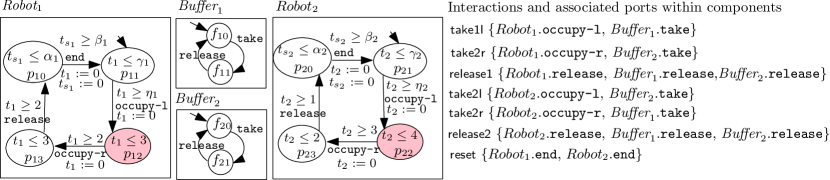
Figure 1: Parametric robot stations with shared buffer locations.

The concrete semantics of a system under a valuation of the unknown parameters follows the standard semantics of timed automata [alur1994tta], except that discrete jumps are synchronized by interactions (see [AstefanoaeiRBBC14] for details). A time run is a maximal sequence of transitions $(\vec{q}_{0},\vec{v}_{0})\stackrel{{\scriptstyle\sigma_{0}}}{{\rightarrow}}(\vec{q}_{1},\vec{v}_{1})\stackrel{{\scriptstyle\sigma_{1}}}{{\rightarrow}}\dots(\vec{q}_{n},\vec{v}_{n})\stackrel{{\scriptstyle\sigma_{n}}}{{\rightarrow}}(\vec{q}_{n+1},\vec{v}_{n+1})\dots$ where $\vec{q}_{i}$ denotes a location in the system $\mathcal{S}$, $\sigma_{i}$ is an interaction and $\vec{v}_{i}$ is a valuation of the clocks in $\mathcal{S}$.

For the ease of reference, we introduce the following notations. For $\sigma\in\Sigma$, we denote $\textit{en}^{t}({\sigma})$ to be the necessary condition for enabling a location combination to trigger $\sigma$ by only allowing finite-time evolving, where the definition of $\textit{en}^{t}({\sigma})$ is taken from [tripakis99:progress]. If from a location $q$ one can delay the triggering of $\sigma$ indefinitely, then $\textit{en}^{t}({\sigma})$ for that location is by default false. Given a valuation $\vec{v}$ assigning the variables in $V$, $\mathcal{S}(\vec{v})$ denotes the resulting concrete timed system and $\textit{en}^{t}({\sigma})(\vec{v})$ denotes the resulting constraint of enabling conditions. For infinite time runs $\rho$ with infinite discrete jumps, we use $\rho_{\Sigma}$ to denote the corresponding $\omega$-word with symbols from the interaction alphabet.

Figure 1 illustrates these concepts by means of a variation of the resource contention problem in terms of timed-based control over robots, which is used as a running example.

Example 1

Given $n$ robots, robot $i$ first accesses buffer $i$ then buffer $(i-1)\%n$. Figure 1 depicts the system for $n=2$, with the set of unknown parameters $V=\{\alpha_{1},\alpha_{2},\beta_{1},$ $\beta_{2},\gamma_{1},\gamma_{2},\eta_{1},\eta_{2}\}$. Each $\textit{Robot}_{i}$ has four ports {occupy-l, occupy-r, release, end}. This system has the interactions $\Sigma=\{{\small\textsf{take1l}},{\small\textsf{take1r}},{\small\textsf{release1}},{\small\textsf{take2l}},$ ${\small\textsf{take2r}},{\small\textsf{release2}},{\small\textsf{reset}}\}$, and $\Delta$ is defined to the right of Figure 1. For $\textit{en}^{t}({{\small\textsf{release1}}})$, the necessary condition for interaction release1 to eventually take place without discrete jumps, is $p_{13}\wedge f_{11}\wedge f_{21}\wedge(t_{1}\leq 3)\wedge(2-t_{1}\leq 3-t_{1})\wedge(3-t_{1}\leq\alpha_{1}-t_{s_{1}})\wedge\delta_{\textit{Robot}_{2}}$. The trivial condition $2-t_{1}\leq 3-t_{1}$ is to guarantee that the minimum required time for $t_{1}$ to have the guard enabled does not let the location invariant of $p_{13}$ be violated. Constraint $3-t_{1}\leq\alpha_{1}-t_{s_{1}}$ is to ensure that the latest delay for enabling the transition, i.e., time elapse of $t_{1}$ to reach the boundary of invariant (which is larger than $2-t_{1}$, the shortest delay required to enable the guard), is less than the time it takes $t_{s_{1}}$ to reach $\alpha_{1}$. This makes it possible to jump to location $p_{10}$. Constraint $\delta_{\textit{Robot}_{2}}=(p_{20}\wedge 3-t_{1}\leq\alpha_{2}-t_{s_{2}})\vee(p_{21}\wedge 3-t_{1}\leq\gamma_{2}-t_{2})\vee(p_{22}\wedge 3-t_{1}\leq 4-t_{2})\vee(p_{23}\wedge 3-t_{1}\leq 2-t_{2})$ is to ensure that $\textit{Robot}_{2}$ is able to stay within its location, before the discrete jump is taken. Note that the clock condition at $p_{13}$ involved in the interaction release1 ensures that time cannot be delayed at infinity.

Now, consider the assignment $\vec{v}\stackrel{{\scriptstyle\triangle}}{{=}}\{\alpha_{1}=\beta_{1}=\alpha_{2}=\beta_{2}=30,\gamma_{1}=5,\gamma_{2}=20,\eta_{1}=0,\eta_{2}=15\}$, which results in an infinite behavior on the interaction level, as presented by the $\omega$-word $\rho_{\Sigma}$: $({\small\textsf{take1l}}\,{\small\textsf{1take1r}}\,{\small\textsf{release1}}\,{\small\textsf{take2l}},{\small\textsf{take2r}}\,{\small\textsf{release2}}\,{\small\textsf{reset}})^{\omega}$.

Definition 3 (Properties)

We consider three types of properties:

• Component-level properties $\phi_{C}$ are constraints over $V$.

• Safety properties $\phi_{state}$ are state properties to be satisfied in every reachable state of the system. Typically, they are location-wise and express relations between clocks.

• Interaction-level properties $\phi_{int}$ are LTL specifications over $\Sigma$. A concrete timed system $\mathcal{S}(\vec{v})$ satisfies $\phi_{int}$ iff every time run $\rho$ of $\mathcal{S}(\vec{v})$ involves infinitely many discrete jumps, and the corresponding $\omega$-word $\rho_{\Sigma}$ is contained in $\phi_{int}$ by standard LTL semantics.

Example 2

Consider the following properties to be synthesized for the robot running example as displayed in Figure 1:

• All parameters should be within $[0,30]$ [Component-level property].

• Deadlock freedom [Safety property].

• $t_{1}+t_{2}$ should always be less than 60 [Safety property].

• Promptness / exclusiveness: $\phi_{prompt}:=\bigwedge_{i}\textbf{G}({\small\textsf{take}}_{i}{\small\textsf{l}}\rightarrow\textbf{X}\bigwedge_{j\neq i}\neg{\small\textsf{take}}_{j}{\small\textsf{l}})$, i.e., disallow $\textit{Robot}_{j}$ to perform ${\small\textsf{take}}_{j}{\small\textsf{l}}$ immediately after ${\small\textsf{take}}_{i}{\small\textsf{l}}$ from $\textit{Robot}_{i}$ [Interaction-level property].

Definition 4 (Timed Orchestration Synthesis)

Given $\mathcal{S}=(V,C,\Sigma,\Delta)$ and properties $\phi_{C}$, $\phi_{state}$, $\phi_{int}$, the problem of timed orchestration synthesis is to find an assignment $\vec{v}$ for $V$ such that $\vec{v}$ satisfies $\phi_{C}$, and $\mathcal{S}(\vec{v})$ satisfies both $\phi_{state}$ and $\phi_{int}$; such a satisfying assignment $\vec{v}$ is also called a solution.

For example, the assignment given in Example 1 is a solution for timed orchestration synthesis when applied to our running example.

3 Timed Orchestration Synthesis

This section describes our main constructions for solving timed orchestration synthesis problems. We first translate timed orchestration synthesis problems for LTL properties to corresponding synthesis problems for safety properties (Sec. 3.1). Second, $\exists\forall$SMT constraints are generated for the latter problem, whereby existential variables quantify over the parameters to be synthesized and universal variables quantify over system states (Sec. LABEL:sub.sec.parameterized.invariants). Third, the $\exists\forall$SMT constraints are solved by means of two alternating quantifier-free SMT solvers (Sec. LABEL:sub.sec.efsmt) for each polarity. In order to simplify the exposition below, we omit $\phi_{C}$ as it ranges only over the existentially-quantified parameters in $V$, and concentrate on the properties $\phi_{state}$ and $\phi_{int}$.

3.1 Transforming Interaction-level to Safety Properties

To effectively synthesize parameters such that interaction-level properties $\phi_{int}$ are satisfied, we adapt bounded LTL synthesis [ScheweF07a] to our context. The underlying strategy is to construct a deterministic progress monitor from $\phi_{int}$. The monitor is meant to keep track of the final states visited in the Büchi automaton $\mathcal{A}_{\neg\phi_{int}}$ corresponding to $\neg\phi_{int}$ during system execution. To achieve this, we equip the monitor with a dedicated risk state representing that a final state in $\mathcal{A}_{\neg\phi_{int}}$ has been visited for $k$ times. When the risk state is never reached for all possible runs, all final states in $\mathcal{A}_{\neg\phi_{int}}$ are visited finitely often (i.e., less than $k$ times). This observation is sufficient to conclude that the system satisfies $\phi_{int}$. This is the intuition behind Algorithm 1.

Algorithm 1 uses $\Sigma_{\phi_{int}}\subseteq\Sigma$ to be the set of interactions from $\phi_{int}$ and $\#$ as a symbol not within $\Sigma$. On Line 4, the symbol $\#$ is used to mark labels corresponding to interactions $\sigma$ not appearing in $\phi_{int}$. On Line 5 a deterministic progress monitor is constructed $C_{\neg\phi_{int},k}$ by unrolling $\mathcal{A}_{\neg\phi_{int}}$ via function $\textbf{monitor}(\mathcal{A}_{\neg\phi_{int}},k)$, which is similar to the approach in bounded LTL synthesis [ScheweF07a]. Consequently, we omit it and instead provide a high-level description of what it does (see below example for understanding): Starting from the initial state of $\mathcal{A}_{\neg\phi_{int}}$, $\Sigma_{\phi_{int}}\cup\{\#\}$ is used to unroll all traces of $\mathcal{A}_{\neg\phi_{int}}$ and to create a deterministic monitor $C_{\neg\phi_{int},k}$. Each location in $C_{\neg\phi_{int},k}$ records the set of states being visited in the Büchi automaton. For each location, the number of times a final state in $\mathcal{A}_{\neg\phi_{int}}$ has been visited previously is counted. The algorithm maintains a queue of unprocessed locations. For each unprocessed location in the queue, every interaction $\sigma\in\Sigma_{\phi_{int}}\cup\{\#\}$ is selected to create a successor location respectively. A state $s^{\prime}$ is stored in the successor location, if state $s$ is in the unprocessed location and if in the post-processed Büchi automaton, a transition from $s$ to $s^{\prime}$ via edge labeled $\sigma$ exists. In addition, the number of visited final states is updated. Whenever a final state in $\mathcal{A}_{\neg\phi_{int}}$ has been visited $k$ times, the unroll process replaces the location of $C_{\neg\phi_{int},k}$ by risk, a dedicated location with no outgoing edges.

Once the monitor is constructed, an augmented system $\mathcal{S}_{inv,k}$ is created from $\mathcal{S}$ (Line 7). The interaction set in the augmented system $\mathcal{S}_{inv,k}$ is the one from Line 6 where all property-unrelated interactions $\sigma$ are marked with $\#$. Finally, on Line 8 the state predicate $\phi_{deadlock}$ expressing the deadlock condition is constructed from the new set of interactions.

Algorithm 1 Translate $\phi_{int}$ into $\phi_{deadlock}$ and construct a monitored system $\mathcal{S}_{inv,k}$

1:Input: $\mathcal{S}$, $\phi_{int}$, $k$

2:Output: $\mathcal{S}_{inv,k},\phi_{deadlock}$

3:construct a Büchi automaton $\mathcal{A}_{\neg\phi_{int}}$ for the negated property of $\phi_{int}$

4:postprocess $\mathcal{A}_{\neg\phi_{int}}$ by replacing every label $\neg\sigma$ with $\Sigma_{\phi_{int}}\setminus\{\sigma\}\cup\{\#\}$

5:$C_{\neg\phi_{int},k}:=$ monitor($\mathcal{A}_{\neg\phi_{int}},k$)

6:$\Delta_{inv,k}(\sigma):=$ $\sigma\in\Sigma_{\phi_{int}}$ ? $\Delta(\sigma)\cup\{C_{\neg\phi_{int},k}.\sigma\}$ : $\Delta(\sigma)\cup\{C_{\neg\phi_{int},k}.\#\}$

7:$\mathcal{S}_{inv,k}=(V,C\cup\{C_{\neg\phi_{int},k}\},\Sigma,\Delta_{inv,k})$

8:$\phi_{deadlock}:=\bigwedge_{\sigma\in\Sigma}\neg\textit{en}^{t}({\sigma})$

9:return $\mathcal{S}_{inv,k}$, $\phi_{deadlock}$

Example 3

We illustrate the steps of the algorithm 1 using the robot running example. Figure 2-(a) illustrates the result $\mathcal{A}_{\neg\phi_{prompt}}$ for property $\phi_{prompt}$ (Line 3), and (b) displays the result after post-processing (Line 4).

To illustrate the result of unrolling in Line 5, Figure 2-(c) shows it for $k=1$. There, the initial location stores {$s_{0}$[$s_{3}$(0)]}, where [$s_{3}$(0)] is to indicate that at $s_{0}$, one has not yet reached $s_{3}$ previously. When the initial location {$s_{0}$[$s_{3}(0)$]} takes interaction take1l, it goes to {$s_{0}$[$s_{3}(0)$], $s_{1}$[$s_{3}(0)$]}, as in Figure 2-(b), state $s_{0}$ can move to $s_{0}$ or $s_{1}$. Notice that it a destination location has possibly been created previously. For example, in Figure 2-(c), for the initial location {$s_{0}$[$s_{3}(0)$]} to take interaction #, it goes back to {$s_{0}$[$s_{3}(0)$]}. For {$s_{0}$[$s_{3}(0)$], $s_{1}$[$s_{3}(0)$]} to take interaction take2l, it moves to a new location {$s_{0}$[$s_{3}(0)$], $s_{3}$[$s_{3}(1)$], $s_{2}$[$s_{3}(0)$]}. This new location is then replaced by risk, as in this example, we have $k=1$.

As for the new interaction set in the monitored system, we show two examples with respect to whether the interaction is in $\phi_{prompt}$:

$$\Delta_{inv,k}({\small\textsf{take1l}})=\{\textit{Robot}_{1}.{\small\textsf{occupy1-l}},\textit{Buffer}_{1}.{\small\textsf{take}},C_{\neg\phi_{prompt}}.{\small\textsf{take1l}}\}$$

$$\Delta_{inv,k}({\small\textsf{take2r}})=\{\textit{Robot}_{2}.{\small\textsf{occupy2-r}},\textit{Buffer}_{1}.{\small\textsf{take}},C_{\neg\phi_{prompt}}.\#\}$$

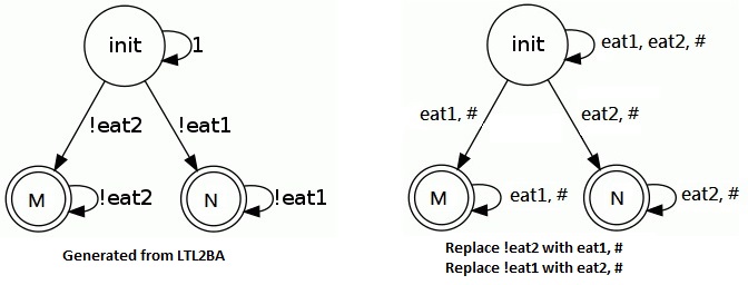
Figure 2: (a)(b) Büchi automaton for $\neg\phi_{prompt}$ before and after postprocessing. (c) $\mathcal{C}_{\neg\phi_{prompt},1}$.

Notice that the introduction of $\#$ symbol simplifies the unroll construction in bounded synthesis. Another difference to vanilla bounded synthesis is that, in the context of unrolling, every state has outgoing edges of size $|\Sigma_{\phi_{int}}\cup\{\#\}|$. In contrast, in bounded LTL synthesis, each $\sigma$ is viewed as a Boolean variable, which creates, in the worst case, on the order of $2^{|\Sigma|}$ outgoing edges.

The following result reduces timed orchestration synthesis for interaction-level properties to a corresponding timed orchestration synthesis problem on state-based properties only.

Lemma 1

Given $\vec{v}$ an assignment of $V$, $\mathcal{S}(\vec{v})$ satisfies $\phi_{int}$ if all time runs of $\mathcal{S}_{inv,k}(\vec{v})$ reach neither the location risk in $C_{\neg\phi_{int},k}$ nor a state where $\phi_{deadlock}(\vec{v})$ holds.

Proof

(Sketch) Assume that any time run $\rho$ in $\mathcal{S}_{inv,k}(\vec{v})$ does not visit location risk or any state where $\phi_{deadlock}(\vec{v})$ holds. We need to show that $\mathcal{S}(\vec{v})$ satisfies $\phi_{int}$.

1. Because $\phi_{deadlock}(\vec{v})$ does not hold and because time runs are maximal, any such time run $\rho$ is infinite.

2. From an infinite time run $\rho$, we show that $\rho$ defines an $\omega$-word $\rho_{\Sigma}$: as $\phi_{deadlock}(\vec{v})$ is never reached, $\bigvee_{\sigma\in\Sigma}\textit{en}^{t}({\sigma})(\vec{v})$ is an invariant for all reachable states. Recall that $\textit{en}^{t}({\sigma})$ is the necessary condition for enabling a location to trigger $\sigma$ by only allowing finite-time evolving. Therefore, for all reachable states, one of the interaction (discrete jump) must appear after finite time. Thus, $\rho$ contains infinitely many discrete jumps and consequently, $\rho$ defines an $\omega$-word $\rho_{\Sigma}$.

3. By construction, every location in the monitor has edges labeled in $\sigma\in\Sigma_{\phi_{int}}\cup\{\#\}$, and # marks each property-unrelated interaction in $\Sigma\setminus\Sigma_{\phi_{int}}$ (Line 6). From this observation, together with the fact that $\mathcal{S}_{inv,k}(\vec{v})$ does not restrict the behavior of $\mathcal{S}(\vec{v})$, we have that a time run $\rho$ in $\mathcal{S}_{inv,k}(\vec{v})$ not reaching risk is bisimilar to a time run $\rho^{\prime}$ in $\mathcal{S}(\vec{v})$, with $\rho$ and $\rho^{\prime}$ defining the same $\omega$-word $\rho_{\Sigma}$.

4. Recall that $C_{\neg\phi_{int},k}$ is an unroll of $\mathcal{A}_{\neg\phi_{int}}$. From this, together with the existence of $\rho_{\Sigma}$ and the fact that while running $\rho_{\Sigma}$ in $\mathcal{A}_{\neg\phi_{int}}$ no final state is reached infinitely many times, we have that $\rho_{\Sigma}$ does not satisfy $\neg\phi_{int}$. Consequently, we can conclude that for every time run $\rho^{\prime}$ in $\mathcal{S}(\vec{v})$, the corresponding $\rho_{\Sigma}$ satisfies $\phi_{int}$. ∎

By Lemma 1, it is sufficient to only consider safety properties when performing orchestration synthesis. Notice howerver that, if for a given fixed $k$ Lemma 1 fails for all possible assignments $\vec{v}$ then one may not conclude that no solution exists for the orchestration synthesis problem as there might be a larger $k$ for which Lemma 1 does hold.

Next we show that it is futile to go beyond a reasonable bound. More precisely, if the domains of the parameters in the input system $\mathcal{S}$ are bounded, then one can effectively compute a limit $k^{*}$ on $k$ such that: if Lemma 1 is not applicable for $k^{*}$ then it is also not applicable for any strictly larger $k$.

Lemma 2

Let all parameters in $\mathcal{S}$ have bounded integer domains with common upper bound $\lambda$ and $\delta$ be the number of regions in $\mathcal{S}$ when all parameters within the location and guard conditions are assigned $\lambda$. Let $|\mathcal{A}_{\neg\phi_{int}}|$ be the number of locations in $\mathcal{A}_{\neg\phi_{int}}$, and $\eta$ be the number of discrete location combinations in $\mathcal{S}$, i.e., $\eta=|Q_{1}||Q_{2}|\dots|Q_{m}|$. Finally, let $k^{*}=\delta^{2}\eta^{2}|\mathcal{A}_{\neg\phi_{int}}||\Sigma|+1$.

Given $\vec{v}$ an assignment of $V$, if there exists a time run of $\mathcal{S}_{inv,k^{*}}(\vec{v})$ reaching either risk in $C_{\neg\phi_{int},k^{*}}$ or a state where $\phi_{deadlock}(\vec{v})$ holds, then $\mathcal{S}(\vec{v})$ does not satisfy $\phi_{int}$.