On Bimaximal Neutrino Mixing and GUT’s

Abstract:

We briefly discuss the present status of models of neutrino mixing. Among the existing viable options we review the virtues of Bimaximal Mixing (that could be implemented by an $S_{4}$ discrete symmetry), corrected by terms arising from the charged lepton mass diagonalization. In particular in a GUT formulation the property of quark lepton ”weak” complementarity can be naturally realized. We discuss in some detail two new versions of particular GUT models, one based on $SU(5)$ and one on $SO(10)$ and the associated phenomenology. We compare these approaches based on symmetry to models based on chance, like Anarchy or $U(1)_{FN}$.

1 Introduction

A long list of models have been formulated over the years to understand neutrino mixing. With time and the continuous improvement of the data most of the models have been discarded by experiment. But the surviving models still span a wide range going from a maximum of symmetry, as those with discrete non-abelian flavour groups (for reviews, see, for example, Refs. [1, 2, 3]), to the opposite extreme of Anarchy [4, 5, 6].

Among the models with a non trivial dynamical structure those based on discrete flavour groups were motivated by the fact that the data suggest some special mixing patterns as good first approximations like Tri-Bimaximal (TB) or Golden Ratio (GR) or Bi-Maximal (BM) mixing, for example. The corresponding mixing matrices all have $\sin^{2}{\theta_{23}}=1/2$, $\sin^{2}{\theta_{13}}=0$, values that are good approximations to the data (although less so since the most recent data), and differ by the value of the solar angle $\sin^{2}{\theta_{12}}$ (see Fig. 1). As the corresponding mixing matrices have the form of rotations with fixed special angles one is naturally led to discrete flavour groups. The relatively large measured value of $\sin{\theta_{13}}$ has disfavoured TB and GR models because they in general predict $\sin{\theta_{13}}$ of the same order as the shift of the predicted $\sin^{2}{\theta_{12}}$ from the observed value, which shift is small for these mixing patterns. Instead in most models of BM the measured value of $\theta_{13}\sim 9^{\circ}$ [7] is natural.

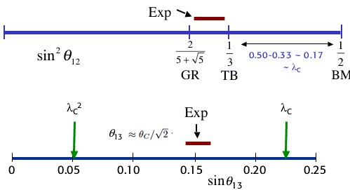
Figure 1: Top: the experimental value of $\sin^{2}{\theta_{12}}$ is compared with the predictions of exact Tri-Bimaximal (TB) or Golden Ratio (GR) or Bi-Maximal mixing (BM). The shift needed to bring the TB or the GR predictions to agree with the experimental value is small, numerically of order $\lambda_{C}^{2}$, while it is larger, of order $\lambda_{C}$ for the BM case, where $\lambda_{C}\equiv\sin{\theta_{C}}$ with $\theta_{C}$ being the Cabibbo angle. Bottom: the experimental value of $\sin{\theta_{13}}$ in comparison with $\lambda_{C}$ or $\lambda_{C}^{2}$.

After the measurement of a relatively large value for $\theta_{13}$ there has been an intense work to interpret the new data along different approaches and ideas. Examples are suitable modifications of the minimal TB models [8, 9], modified sequential dominance models [10], larger symmetries that already at LO lead to non vanishing $\theta_{13}$ and non maximal $\theta_{23}$ [11], smaller symmetries that leave more freedom [12], models where the flavour group and a generalised CP transformation are combined in a non trivial way [13] (other approaches to discrete symmetry and CP violation are found in Refs. [14]).

Among discrete symmetry models, now that the value of $\sin^{2}{\theta_{13}}$ has been measured and found to be not so small ([15]-[18]) the interest on BM mixing has been boosted [19, 20]. In this case the neutrino mixing matrix before diagonalization of charged leptons has $\sin^{2}{\theta_{12}}$ and $\sin^{2}{\theta_{23}}$ both maximal and $\sin{\theta_{13}=0}$. The BM mixing matrix is in fact:

$$U_{BM}=\left(\begin{array}[]{ccc}\displaystyle\frac{1}{\sqrt{2}}&\displaystyle-\frac{1}{\sqrt{2}}&0\\ \displaystyle\frac{1}{2}&\displaystyle\frac{1}{2}&-\displaystyle\frac{1}{\sqrt{2}}\\ \displaystyle\frac{1}{2}&\displaystyle\frac{1}{2}&\displaystyle\frac{1}{\sqrt{2}}\end{array}\right)\;.$$ (1)

The most general mass matrix corresponding to this mixing matrix is:

$$m_{\nu BM}=\left(\begin{array}[]{ccc}x&y&y\\ y&z&x-z\\ y&x-z&z\end{array}\right)\;,$$ (2)

where $x$,$y$ and $z$ are three complex numbers. One can think of a suitable symmetry or of some other dynamical ingredient that enforces BM mixing in the neutrino sector and that the necessary, rather large, corrective terms to $\theta_{12}$ and $\theta_{13}$ arise from the diagonalization of the charged lepton mass matrix. As well known, BM corrected by charged lepton diagonalization can be obtained in models based on the discrete symmetry $S_{4}$ [21, 22]. This idea is in line with the well-known empirical observation that $\theta_{12}+\theta_{C}\sim\pi/4$, where $\theta_{C}$ is the Cabibbo angle, a relation known as quark-lepton complementarity [23]-[26]. Probably the exact complementarity relation becomes more plausible if replaced by $\theta_{12}+\mathcal{O}(\theta_{C})\sim\pi/4$ (which we call “weak” complementarity). In addition the measured value of $\theta_{13}$ is itself of order $\theta_{C}$: $\theta_{13}\sim\theta_{C}/\sqrt{2}$. The relation of the neutrino mixing angles with $\theta_{C}$ could well arise in Grand Unified (GUT) models [26, 27] so that we will focus on GUT models in this work.

In the present note we discuss two examples of GUT models of BM, one based on $SU(5)$ and one on $SO(10)$. The $SU(5)$ model discussed here is more complete and indeed is based on a broken flavour symmetry that contains $S_{4}$ which imposes the BM structure in the neutrino sector and is then corrected by terms arising from the diagonalization of charged lepton masses. The present $SU(5)$ model has the virtue that the quark mixing angles and the shifts from the BM values in the neutrino sector, all turn out to be naturally of the correct order of magnitude, expressed in terms of powers of $\lambda_{C}=\sin{\theta_{C}}$, a’ la Wolfenstein, modulo coefficients of $\mathcal{O}(1)$. The $SO(10)$ model is based on Type-II see-saw and the origin of BM before diagonalization of charged leptons is in this case left unspecified. Both GUT theories discussed in the following are variants of models already appeared in the literature, in particular by our group [22, 28]. We discuss the phenomenology of these models in the context of the present data and the comparison with other approaches like Anarchy and $U(1)_{FN}$ models.

On the other hand, the relatively large measured value of $\theta_{13}$, close in size to the Cabibbo angle, and the indication that $\theta_{23}$ is not maximal both go in the direction of models based on Anarchy, i.e. the idea that perhaps no symmetry is needed in the neutrino sector, only chance. The appeal of Anarchy is augmented if formulated in a $SU(5)\otimes U(1)_{FN}$ context with different Froggatt-Nielsen [29] charges only for the $SU(5)$ tenplets (for example $10\sim(a,b,0)$, where $a>b>0$ is the charge of the first generation, $b$ of the second, zero of the third) while no charge differences appear in the $\bar{5}$ (e. g. $\bar{5}\sim(0,0,0)$). In fact, the observed fact that the up-quark mass hierarchies are more pronounced than for down-quarks and charged leptons is in agreement with this assignment. Indeed the embedding of Anarchy in the $SU(5)\otimes U(1)_{FN}$ context allows to implement a parallel treatment of quarks and leptons. Note that implementing Anarchy and its variants in $SO(10)$ would be difficult due to the fact that all left-handed Standard Model (SM) fields of one generation belong to the same spinoral representation $16$. In models with no see-saw, the $\bar{5}$ charges completely fix the hierarchies (or Anarchy, if the case) in the neutrino mass matrix. If RH neutrinos are added, they transform as $SU(5)$ singlets and can in principle carry independent $U(1)_{FN}$ charges, which also, in the Anarchy case, must be all equal. With RH neutrinos the see-saw mechanism can take place and the resulting phenomenology is modified.

The $SU(5)$ generators act vertically inside one generation, whereas the $U(1)_{FN}$ charges differ horizontally from one generation to the other. If, for a given interaction vertex, the $U(1)_{FN}$ charges do not add to zero, the vertex is forbidden in the symmetric limit. However, the $U(1)_{FN}$ symmetry (that one can assume to be a gauge symmetry) is spontaneously broken by the VEVs $v_{f}$ of a number of flavon fields with non-vanishing charge and GUT-scale masses. Then a forbidden coupling is rescued but is suppressed by powers of the small parameters $\lambda=v_{f}/M$, with $M$ a large mass, with the exponents larger for larger charge mismatch. Thus the charges fix the powers of $\lambda$, hence the degree of suppression of all elements of mass matrices, while arbitrary coefficients $k_{ij}$ of order 1 in each entry of mass matrices are left unspecified (so that the number of order 1 parameters largely exceeds the number of observable quantities). A random selection of these $k_{ij}$ parameters leads to distributions of resulting values for the measurable quantities. For Anarchy the mass matrices in the neutrino sector (determined by the $\bar{5}$ and $1$ charges) are totally random, while in the presence of unequal charges different entries carry different powers of the order parameter and thus suitable hierarchies are enforced for quarks and charged leptons by unequal tenplet charges. Within this framework there are many variants of models largely based on chance: fermion charges can all be non-negative with only negatively charged flavons, or there can be fermion charges of different signs with either flavons of both charges or only flavons of one charge. In Refs.[30, 31], given the new experimental results, a reappraisal of Anarchy and its variants within the $SU(5)\times U(1)_{\rm FN}$ GUT framework was made. Based on the most recent data it is argued that the Anarchy ansatz is probably oversimplified and, in any case, not compelling. In fact, suitable differences of $U(1)_{FN}$ charges, if also introduced within pentaplets and singlets, lead, with the same number of random parameters as for Anarchy, to distributions that are in better agreement with the data.

2 A SUSY $SU(5)$ model with $S_{4}$ discrete symmetry

This model is a variant of those of Refs.[21, 22] to which we refer the reader for a detailed discussion and the technical details [32]-[35]. Here we concentrate on the differences, the motivations and the resulting phenomenology. This is a SUSY $SU(5)$ model in 4+1 dimensions with a flavour symmetry $S_{4}\otimes Z_{3}\otimes U(1)_{R}\otimes U(1)_{FN}$, where $U(1)_{R}$ implements the R-symmetry while $U(1)_{FN}$ is a Froggatt-Nielsen (FN) symmetry [29] that induces the hierarchies of fermion masses and mixings. The particle assignments are displayed in Tab.1.

Field	$F$	$T_{1}$	$T_{2}$	$T_{3}$	$H_{5}$	$H_{\overline{5}}$	$\varphi_{\nu}$	$\xi_{\nu}$	$\varphi_{\ell}$	$\chi_{\ell}$	$\theta$	$\theta^{\prime}$	$\varphi^{0}_{\nu}$	$\xi^{0}_{\nu}$	$\psi^{0}_{\ell}$	$\chi^{0}_{\ell}$
SU(5)	$\bar{5}$	10	10	10	5	${\overline{5}}$	1	1	1	1	1	1	1	1	1	1
$S_{4}$	$3_{1}$	1	1	1	1	1	$3_{1}$	1	$3_{1}$	$3_{2}$	1	1	$3_{1}$	1	2	$3_{2}$
$Z_{3}$	$\omega$	$\omega$	1	$\omega^{2}$	$\omega^{2}$	$\omega^{2}$	1	1	$\omega$	$\omega$	1	$\omega$	1	1	$\omega$	$\omega$
$U(1)_{R}$	1	1	1	1	0	0	0	0	0	0	0	0	2	2	2	2
$U(1)_{FN}$	0	2	1	0	0	0	0	0	0	0	-1	-1	0	0	0	0
	br	bu	bu	br	bu	bu	br	br	br	br	br	br	br	br	br	br

Table 1: Matter assignment of the model. The symbol ${\tt br}({\tt bu})$ indicates that the corresponding fields live on the brane (bulk).

The formulation in 4+1 dimensions, with coordinate $y$ in the fifth dimension compactified on a circle, allows a more efficient realization of GUT with less Higgs states, no doublet-triplet splitting problem and a better control of proton decay. In the present model it also introduces some extra hierarchy for some of the couplings. In fact, as indicated in the table, some of the particles are in the bulk (the first two generation tenplets $T_{1}$ and $T_{2}$ and the Higgs $H_{5}$ and $H_{\bar{5}}$) while all the other ones are on the brane at $y=0$. Actually, to obtain the correct zero mode spectrum, one must introduce two copies, $T_{1,2}$ and $T^{\prime}_{1,2}$ with opposite orbifolding parity. The zero modes of $T_{1,2}$ are the quark doublets $Q_{1,2}$, while those of $T^{\prime}_{1,2}$ are $U^{c}_{1,2}$ and $E^{c}_{1,2}$. For economy of space only $T_{1,2}$ appear in table 1. At leading order (LO) the $S_{4}$ symmetry is broken down to suitable different subgroups in the charged lepton sector and in the neutrino sector by the VEV’s of the flavons $\varphi_{\nu}$, $\xi_{\nu}$, $\varphi_{\ell}$ and $\chi_{\ell}$. The necessary proper alignment of the VEV’s is implemented, in a natural way, by the driving fields $\varphi^{0}_{\nu}$, $\xi^{0}_{\nu}$, $\psi^{0}_{\ell}$, $\chi^{0}_{\ell}$. The VEVs of the $\theta$ and $\theta^{\prime}$ fields break the FN symmetry. As a result, at LO the charged lepton masses are diagonal and exact BM is realized for neutrinos. Corrections to diagonal charged leptons and to exact BM are induced by vertices of higher dimension in the Lagrangian, suppressed by powers of a large scale $\Lambda$. While broken $S_{4}$ is at the origin of BM, $U(1)_{FN}$, together with some higher dimensional effects, fixes the hierarchies of quark and charged lepton masses.

With respect to Ref.[22] here we have modified the FN charges of the tenplets from (3,1,0) to (2,1,0). With this choice we aim at optimizing the neutrino mixing angles and to implement the ”weak complementarity” relation at the expenses of a less accurate description of the first generation quark and charged lepton masses. We adopt the definitions:

$$\frac{v_{\varphi_{\ell}}}{\Lambda}\sim\frac{v_{\chi}}{\Lambda}\sim\epsilon^{\prime}\;;\qquad\frac{v_{\varphi_{\nu}}}{\Lambda}\sim\frac{v_{\xi}}{\Lambda}\sim\epsilon\;,$$ (3)

$$\frac{\langle\theta\rangle}{\Lambda}=t\qquad\frac{\langle\theta^{\prime}\rangle}{\Lambda}=t^{\prime}\,.$$ (4)

and

$$s\equiv\displaystyle\frac{1}{\sqrt{\pi R\Lambda}}<1~{}~{}~{}.$$ (5)

where $s$ is the volume suppression factor.

It turns out that the simplest choice of setting all these parameters to be of $\mathcal{O}(\lambda\sim\lambda_{C})$:

$$s=\epsilon=\epsilon^{\prime}=t=t^{\prime}=\lambda_{C},$$ (6)

leads to a good description of masses and mixings, as described below. Indeed by proceeding in exact analogy with Ref.[22], we have the following results.

2.1 Down quarks and charged lepton mass matrices

For the down quark mass matrix, by only keeping the leading terms for each entry, one finds:

$$m_{d}=\left(\begin{array}[]{ccc}a_{11}\lambda^{5}&a_{12}\lambda^{4}&a_{13}\lambda^{4}\\ a_{21}\lambda^{4}&-c\lambda^{3}&c\lambda^{3}\\ a_{31}\lambda^{2}&......&a_{33}\lambda\end{array}\right)\lambda v_{d}^{0}~{}~{}~{}.$$ (7)

Here all matrix elements are multiplied by generic coefficients $a_{ij}$ of $\mathcal{O}(1)$ with the exception of the (22) and (23) entries where the coefficients given by $-c$ and $c$ are equal and opposite. In the (32) entry the dots indicate that the lowest order potentially non vanishing is actually zero and the entry will get a contribution from still higher orders. For example, the entry (11) gets contributions from terms $\mathcal{O}(st\epsilon^{\prime}t^{\prime}\epsilon\sim\lambda^{5})$. Thus the hierarchies arise from a combination of extra dimension factors, $S_{4}$ and $U(1)_{FN}$ breaking. For the mass eigenvalues we have:

$$m_{b}\sim v_{d}^{0}\lambda^{2},~{}~{}~{}~{}~{}~{}~{}m_{s}\sim v_{d}^{0}\lambda^{4},~{}~{}~{}~{}~{}~{}~{}m_{d}\sim v_{d}^{0}\lambda^{6}.$$ (8)

For the charged lepton masses we have to take into account the introduction of the copies $T^{\prime}_{1,2}$ of the first two tenplet fields, whose zero modes are different from those of $T_{1,2}$ and couple with the charged leptons only. Therefore, all the operators of the form $FT_{3}H_{\overline{5}}$ have exactly the same order 1 coefficients whereas all others containing $T^{\prime}_{1,2}$ have different coefficients. This translates in the following mass matrix:

$$m_{e}=\left(\begin{array}[]{ccc}a_{11}^{\prime}\lambda^{5}&a_{21}^{\prime}\lambda^{4}&a_{31}\lambda^{2}\\ a_{12}^{\prime}\lambda^{4}&-c^{\prime}\lambda^{3}&......\\ a_{13}\lambda^{4}&c^{\prime}\lambda^{3}&a_{33}\lambda\end{array}\right)\lambda v_{d}^{0}~{}~{}~{},$$ (9)

and the charged lepton masses are:

$$m_{\tau}=m_{b}\sim v_{d}^{0}\lambda^{2},~{}~{}~{}~{}~{}~{}~{}m_{\mu}\sim v_{d}^{0}\lambda^{4},~{}~{}~{}~{}~{}~{}~{}m_{e}\sim v_{d}^{0}\lambda^{6}.$$ (10)

Note that the $b-\tau$ universality is realized: here and in the following we obviously refer to masses at the GUT scale as for example given in Ref.[36]. Note that the predicted ratio $m_{e}/m_{\mu}\sim\lambda^{2}$ is not perfect, being too large.

The unitary left-handed rotation $U_{d}$ is obtained diagonalizing $m_{d}\,m_{d}^{\dagger}$ whereas the right-handed one $U_{\ell}$ is the charged lepton rotation. Taking only the largest contribution for each matrix elements, for $U_{\ell}$, which enters in the neutrino mixing matrix, $U_{PNMS}=U_{\ell}^{\dagger}U_{\nu}$ we have:

$$U_{\ell}\sim\left(\begin{array}[]{ccc}1&u_{12}\lambda&u_{13}\lambda\\ -u_{12}^{*}\lambda&1&0\\ -u_{13}^{*}\lambda&-u_{12}^{*}u_{13}^{*}\lambda^{2}&1\\ \end{array}\right)\,,$$ (14)

so that $\theta_{23}^{\ell}=0$ in this approximation.

2.2 Up quarks mass matrix

Similarly the symmetric up quark mass matrix is given by:

$$m_{u}=\left(\begin{array}[]{ccc}b_{11}\lambda^{6}&b_{12}\lambda^{5}&b_{13}\lambda^{3}\\ b_{12}\lambda^{5}&b_{22}\lambda^{4}&b_{23}\lambda^{4}\\ b_{13}\lambda^{3}&b_{23}\lambda^{4}&b_{33}\end{array}\right)\lambda v_{u}^{0}~{}~{}~{},$$ (15)

and the masses are:

$$m_{t}\sim v_{u}^{0}\lambda,~{}~{}~{}~{}~{}~{}~{}m_{c}\sim v_{u}^{0}\lambda^{5},~{}~{}~{}~{}~{}~{}~{}m_{u}\sim v_{u}^{0}\lambda^{7}.$$ (16)

The ratio $m_{b}/m_{t}\sim\lambda v_{d}^{0}/v_{u}^{0}\sim\lambda/\tan\beta$ implies that $\tan\beta\sim 1/\lambda$. In most of the cases the mass ratios are correctly reproduced, but, as already announced, there are some cases that need some moderate fine tuning. For example, we have $m_{u}/m_{c}\sim\lambda^{2}$ which is too large, $m_{u}/m_{d}\sim m_{c}/m_{s}$ where, in reality the two sides differ by a factor of about 25. As we already mentioned we have chosen as a priority to fit the mixings rather than the masses. One can improve the agreement by somewhat relaxing the strict equalities in eq. (6). We now turn to describe the model predictions for the mixings first in the quark sector and then, after discussing the neutrino mass matrix, in the leptonic sector.

2.3 The CKM matrix

The CKM matrix is given by $V_{CKM}=U_{u}^{\dagger}U_{d}$. The leading order expressions for $U_{u}$ and $U_{d}$ obtained from the up and down quark mass matrices in eqs.(7) and (15) are of the form:

$$U_{u}\sim\left(\begin{array}[]{ccc}1&c_{12}\lambda&u_{13}\lambda^{3}\\ -c_{12}^{*}\lambda&1&0\\ -c_{13}^{*}\lambda^{3}&0&1\\ \end{array}\right)\,$$ (20)

and

$$U_{d}\sim\left(\begin{array}[]{ccc}1&d_{12}\lambda&d_{13}\lambda^{3}\\ -d_{12}^{*}\lambda&1&d_{23}\lambda^{2}\\ (d_{12}^{*}d_{23}^{*}-d_{13}^{*})\lambda^{3}&-d_{23}\lambda^{2}&1\\ \end{array}\right)\,.$$ (24)

From these expressions we obtain the leading order form of the $V_{CKM}$ matrix with a pattern of the Wolfenstein type:

$$V_{CKM}\sim\left(\begin{array}[]{ccc}1&v_{12}\lambda&v_{13}\lambda^{3}\\ -v_{12}^{*}\lambda&1&v_{23}\lambda^{2}\\ (v_{12}^{*}v_{23}^{*}-v_{13}^{*})\lambda^{3}&-v_{23}\lambda^{2}&1\\ \end{array}\right)\,.$$ (28)

The $v_{ij}$ coefficients are related to the $c_{ij}$ and $d_{ij}$ coefficients by:

$$v_{12}=d_{12}-c_{12}^{*};~{}~{}~{}~{}~{}v_{13}=(d_{13}-c_{12}^{*}d_{23}-c_{13}^{*});~{}~{}~{}~{}~{}v_{23}=d_{23}.$$ (29)

We see that for $\lambda=\lambda_{C}$ the correct order of magnitude is derived for each $V_{CKM}$ matrix element modulo coefficients generically of order 1.

2.4 The neutrino masses and mixings

The neutrino sector of the model is unchanged with respect to Ref.[22]. We therefore limit ourselves here to recall some important points. First note that in Tab.1 there are no right-handed neutrinos. So the table refers to a model where the neutrino mass matrix is generated by the effective dimension 5 Weinberg operator. But a see-saw version is easily obtained by adding 3 right-handed neutrinos transforming under SU(5)$\times S_{4}\times Z_{3}$ as $(1,3_{1},1)$ and with charges $U(1)_{R}=+1$ and $U(1)_{FN}=0$. The relevant phenomenology is quite similar, in particular the results on neutrino mixing. However, the neutrino mass spectrum turns out to be of moderate normal hierarchy type, with a LO lightest neutrino mass $|m_{1}|$ larger than about 0.01 eV and, consequently, values of $m_{ee}\geq 3-4~{}10^{-3}$ eV. The deviation from a pure BM neutrino mass matrix is responsible for a softening of the lower bound on $|m_{1}|$ and for an enlargement of the allowed values of the $0\nu\beta\beta$ rate. The experimental value of $\sqrt{r}=\sqrt{\frac{\Delta m^{2}_{sol}}{\Delta m^{2}_{atm}}}\sim 1/6$ needs some fine tuning because in the model it should be of $\mathcal{O}(1)$. This fine tuning appears in most discrete symmetry models because neutrinos must be in triplet representations of the discrete group in order to obtain BM or TB mixing etc. and then the mass eigenvalues are all of the same order of magnitude, barring cancellations.

The neutrino mixing matrix is obtained as $U_{\nu}=U_{\ell}^{\dagger}U_{BM}$ where $U_{\ell}$ is given in eq. (14) and $U_{BM}$ is the unitary matrix of BM. The results for the mixing angles are easily derived:

$$\sin{\theta_{13}} = \frac{1}{\sqrt{2}}|u_{12}-u_{13}|\lambda\equiv|\Delta|$$

$$\sin^{2}{\theta_{12}} = \frac{1}{2}-\frac{1}{\sqrt{2}}~{}Re(u_{12}+u_{13})\lambda\equiv\frac{1}{2}-Re\Sigma$$ (30)

$$\sin^{2}{\theta_{23}} = \frac{1}{2}+\mathcal{O}(\lambda^{2})$$

The CP phase $\delta_{CP}$ is

$$\delta_{CP}=\pi+arg(u_{12}-u_{13})\equiv\pi+arg(\Delta).$$ (31)

where the complex numbers $\Delta$ and $\Sigma$ are defined as $\Delta=\frac{1}{\sqrt{2}}|u_{12}-u_{13}|\lambda$ and $\Sigma=\frac{1}{\sqrt{2}}~{}(u_{12}+u_{13})\lambda$. The results are graphically reported in Fig. 2 and compared with the experimental values of $\sin{\theta_{13}}$ and $\sin^{2}{\theta_{12}}$. We see that, with $\lambda\sim\lambda_{C}$, the model realizes the ”weak” complementarity relation and the experimental fact that $\sin{\theta_{13}}$ is of the same order than the shift of $\sin^{2}{\theta_{12}}$ from the BM value of 1/2, both of order $\lambda_{C}$. It is interesting to observe that corrections to the BM pattern arising from next-to-leading order effects in the Yukawa couplings (higher order operators and shifts from LO flavon vevs) only affect $\sin^{2}{\theta_{23}}$ at the same $\mathcal{O}(\lambda^{2})$ as in eq.(30). We also see that, in general, the CP phase $\delta_{CP}$ is not predicted, as the data only fix the absolute value of $\Delta$ and not its phase. If one could neglect $u_{13}$ then $\Delta$ and $\Sigma$ would coincide. A very marginal agreement with the data would then demand that both be aligned along the positive real axis and, in this case $\delta_{CP}=\pi$.

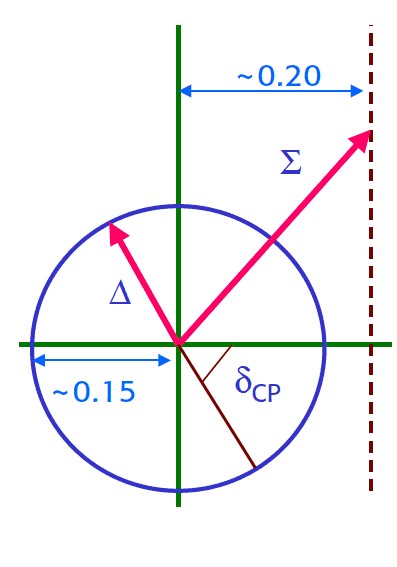
Figure 2: The complex numbers $\Delta=\frac{1}{\sqrt{2}}|u_{12}-u_{13}|\lambda$ and $\Sigma=\frac{1}{\sqrt{2}}~{}(u_{12}+u_{13})\lambda$ determine $\sin{\theta_{13}}=|\Delta|$ and $\sin^{2}{\theta_{12}}=\frac{1}{2}-Re\Sigma$. The CP phase is given by $\delta_{CP}=\pi+arg(\Delta)$. The numbers shown approximately indicate the experimental central values.

3 Comparison with $SU(5)\bigotimes U(1)$ models

It is interesting to compare the previous model, which is rather complicated involving SUSY $SU(5)$, a non abelian $S_{4}$ symmetry and extra dimensions, with a much simpler class of models based on SUSY $SU(5)\otimes U(1)_{FN}$ [29]. As we have explicitly discussed a non see-saw version of the $S_{4}$ model we will compare it with a non see-saw version of the $U(1)_{FN}$ models. In the following, only $U(1)_{FN}$ models with normal hierarchy are considered because, as shown in Ref.[37], $U(1)$ models with inverse hierarchy (IH) tend to favour a solar angle close to maximal.

In general we can label the $U(1)$ charges as follows:

$$10\sim(t_{1},t_{2},0)~{}~{}~{}~{}~{}~{}~{}~{}~{}~{}~{}~{}\bar{5}\sim(f_{1},f_{2},0)\\$$ (32)

where 1, 2 refer to the first and second families. The Higgs field charges are taken as vanishing. There is also a flavon field $\theta$ with charge -1 whose VEV $\langle\theta\rangle$ breaks $U(1)_{FN}$. A set of charge values that lead to a good agreement with the observed masses and mixings are (this is the so-called $A_{\mu\tau}$ case in [38]):

$$10\sim(3,2,0)~{}~{}~{}~{}~{}~{}~{}~{}~{}~{}~{}~{}\bar{5}\sim(1,0,0)\,.\\$$ (33)

The following mass matrices are obtained. For the up-type quarks:

$$m_{u}=\left(\begin{array}[]{ccc}\lambda^{6}&\lambda^{5}&\lambda^{3}\\ \lambda^{5}&\lambda^{4}&\lambda^{2}\\ \lambda^{3}&\lambda^{2}&1\end{array}\right)v_{u}^{0}~{}~{}~{}.$$ (34)

Here $\lambda=\langle\theta\rangle/\Lambda$ with $\Lambda$ the large scale that suppresses the non rinormalizable interactions involving the field $\theta$ and all entries are multiplied by coefficients that are complex numbers with absolute values of order 1.

The down-type quarks and charged lepton mass matrices are one the transposed of the other and are given by:

$$m_{d}=m_{e}^{T}=\left(\begin{array}[]{ccc}\lambda^{4}&\lambda^{3}&\lambda^{3}\\ \lambda^{3}&\lambda^{2}&\lambda^{2}\\ \lambda&1&1\end{array}\right)v_{d}^{0}~{}~{}~{}.$$ (35)

Finally, the neutrino mass matrix transforming as $\bar{5}\otimes\bar{5}$ from the dimension 5 Weinberg operator is given by:

$$m_{\nu}=\left(\begin{array}[]{ccc}\lambda^{2}&\lambda&\lambda\\ \lambda&1&1\\ \lambda&1&1\end{array}\right)\frac{(v_{u}^{0})^{2}}{\Lambda}~{}~{}~{}.$$ (36)

We can now compare the two models starting from quarks and charged leptons. We observe that the structure of the mass matrices is very similar although not identical. In the $S_{4}$ model the suppression factors from the geometry in the extra dimension combine with those from the $U(1)_{FN}$ charges (which are different from those in the abelian model) to produce a similar pattern in the two cases. The mass matrices are not precisely the same in the two models but the predictions for the orders of magnitude of the mass ratios, expressed in terms of powers of $\lambda$ are identical. For both models we have in fact:

$$\frac{m_{u}}{m_{c}}\sim\frac{m_{d}}{m_{s}}\sim\frac{m_{s}}{m_{b}} \sim \frac{m_{e}}{m_{\mu}}\sim\frac{m_{\mu}}{m_{\tau}}\sim\lambda^{2}$$ (37)

$$\frac{m_{c}}{m_{t}} \sim \lambda^{4}$$ (38)

Most of these orders of magnitude are correct if $\lambda\sim\lambda_{C}$ but some, involving the first generation masses, are not, like $m_{u}/m_{c}$, $m_{d}/m_{s}$ and $m_{e}/m_{\mu}$. Although the predictions for the mass ratios are the same, the $S_{4}$ model is superior, because its extra dimensional formulation solves the doublet triplet splitting problem and introduces corrections to the relation $m_{d}=m_{e}^{T}$ of the Georgi-Jarlskog type. Also in the $S_{4}$ model $m_{t}/m_{b}\sim v^{0}_{u}/(\lambda v^{0}_{d})\sim\tan\beta/\lambda$ while the factor $1/\lambda$ is absent in the $U(1)_{FN}$ model, so that only a moderate value of $\tan\beta$ is needed in the $S_{4}$ model. The CKM quark mixing angles are also of the same order of magnitude in the two models and match the Wolfenstein pattern: $\theta_{12}^{q}\sim\lambda$, $\theta_{13}^{q}\sim\lambda^{3}$ and $\theta_{23}^{q}\sim\lambda^{2}$.

In conclusion, in the charged fermion sector the two models are rather comparable, with some advantages for the $S_{4}$ model. But where the latter is definitely superior is in the neutrino sector. As a result of the $S_{4}$ construction, the neutrino mixing pattern is dictated by BM corrected by terms from the diagonalization of charged leptons as detailed in eq.(30). The weak form of complementarity is realized as the shift of $\theta_{12}^{\nu}$ is of the order of $\lambda\sim\lambda_{C}$ and moreover also $\theta_{13}^{\nu}\sim\lambda_{C}$ while $\theta_{23}^{\nu}$ deviates from the maximal value by terms of order $\lambda^{2}$. As already mentioned the observed value of $\sqrt{r}=\sqrt{\frac{\Delta m^{2}_{sol}}{\Delta m^{2}_{atm}}}\sim 1/6$ needs some fine tuning because in the model it should be of $\mathcal{O}(1)$. In the $U(1)_{FN}$ model the neutrino matrix is given in eq.(36). The diagonalization of charged leptons does not alter this pattern. For generic coefficients of $\mathcal{O}(1)$ for each matrix entry, we would get that $\theta_{13}^{\nu}\sim\lambda$, $\theta_{23}^{\nu}\sim\mathcal{O}(1)$ which are good but also $r\sim\mathcal{O}(1)$ and $\theta_{12}^{\nu}\sim\lambda$ which are bad. However, if, by accident, the 22 matrix element of $m_{\nu}$ is of order $\lambda$, then $\sqrt{r}\sim\lambda$ and $\theta_{12}^{\nu}\sim\mathcal{O}(1)$: with a single fine tuning one fixes both problems. In any case, even accepting some amount of fine tuning, clearly there is no realization of weak complementarity. Finally in both models there are far more parameters than observables. This redundancy is less pronounced for the $S_{4}$ model but is still large.

4 Bimaximal mixing in a $SO(10)$ GUT model

A challenging problem is that of formulating a natural model of Grand Unification based on $SO(10)$, leading not only to a good description of quark masses and mixing but also, in addition, of charged lepton masses and neutrino mixing. In $SO(10)$ the main added difficulty with respect to $SU(5)$ is clearly that all fermions in one generation belong to a single 16-dimensional representation, so that one cannot separately play with the properties of the $SU(5)$-singlet right-handed neutrinos in order to explain the striking difference between quark and neutrino mixing. A promising strategy in order to separate charged fermions and neutrinos in $SO(10)$ is to assume the dominance of type-II see-saw [39] (with respect to type-I see-saw [40]) for the light neutrino mass matrix. If type-II seesaw is responsible for neutrino masses, then the neutrino mass matrix (proportional to) $f$ (see eqs.(39,41,42)) is separated from the dominant contributions to the charged fermion masses and can therefore show a completely different pattern. This is to be compared with the case of type-I see-saw where the neutrino mass matrix depends on the neutrino Dirac and Majorana matrices and, in $SO(10)$, the relation with the charged fermion mass matrices is tighter.

In Ref.[28], when the data suggested approximate TB mixing and a small value of $\sin^{2}{\theta_{13}}$, an $SO(10)$ model has been studied based on type-II see-saw dominance. A detailed discussion of the general structure of this class of models can be found in the above article, together with a comparison with other approaches to $SO(10)$ GUT’s. Here, given the relatively large value of $\sin^{2}{\theta_{13}}$ that has been recently measured, we reconsider this type of GUT model in the case of approximate BM mixing corrected by the charged lepton diagonalization.

In renormalizable $SO(10)$ models (a non necessary assumption only taken here for simplicity) the Higgs fields that contribute to fermion masses are in 10 (denoted by $H$), ${\bf\overline{126}}$ ($\overline{\Delta}$) and 120 ($\Sigma$). The Yukawa superpotential of this model is then given by:

$$W_{Y}~{}=~{}h\,\psi\psi H+f\,\psi\psi\bar{\Delta}+h^{\prime}\,\psi\psi\Sigma\,,$$ (39)

where the symbol $\psi$ stands for the 16 dimensional representation of SO(10) that includes all the fermion fields in one generation. The coupling matrices $h$ and $f$ are symmetric, while $h^{\prime}$ is anti-symmetric. The representations $H$ and $\Delta$ have two SM doublets in each of them whereas $\Sigma$ has four such doublets. At the GUT scale $M_{GUT}$, once the GUT and the $B-L$ symmetry are broken, one linear combination of the up-type and one of down-type doublets remain almost massless whereas the remaining combinations acquire GUT scale masses. The electroweak symmetry is broken after the light Minimal Supersymmetric Standard Model (MSSM) doublets (to be called $H_{u,d}$) acquire vacuum expectation values (vevs) and they then generate the fermion masses. The resulting mass formulae for different fermion masses are given by (see, for example, [41]):

$$Y_{u} = h+r_{2}f+r_{3}h^{\prime},$$ (40)

$$Y_{d} = r_{1}(h+f+h^{\prime})\,,$$

$$Y_{e} = r_{1}(h-3f+c_{e}h^{\prime})\,,$$

$$Y_{\nu^{D}} = h-3r_{2}f+c_{\nu}h^{\prime},$$

where $Y_{a}$ are mass matrices divided by the electro-weak vev’s $v_{u,d}$ and $r_{a}$ ($a=1,2,3$ and $c_{b}$ ($b=e,\nu$) are the mixing parameters which relate the $H_{u,d}$ to the doublets in the various GUT multiplets.

In generic $SO(10)$ models of this type, the neutrino mass formula has a type-II and a type-I contribution:

$${\cal M}_{\nu}~{}=~{}fv_{L}-M_{D}\frac{1}{fv_{R}}M^{T}_{D}\,,$$ (41)

where $v_{L}$ is the vev of the $B-L=2$ triplet in the ${\bf\overline{126}}$ Higgs field. Note that in general, the two contributions to neutrino mass depend on two different parameters, $v_{L}$ and $v_{R}$, and it is possible to have a symmetry breaking pattern in $SO(10)$ such that the first contribution (the type-II term) dominates over the type-I term. The possible realisation of this dominance and its consistency with coupling unification has been studied in the literature [42, 43, 44, 45] and found tricky but not impossible [46]. The neutrino mass formula then becomes

$${\cal M}_{\nu}~{}\sim~{}fv_{L}\;.$$ (42)

Note that $f$ is the same coupling matrix that appears in the charged fermion masses in eq. (40), up to factors from the Higgs mixings and the Clebsch-Gordan coefficients. Also note that the neutrino Dirac mass, proportional to $Y_{\nu^{D}}$ in eq. (40), only enters in the neglected type-I see-saw terms and does not play a role in the following analysis. The equations (40) and (42) are the key relations in this approach.

The 10 Yukawa couplings contributing to up, down and charged lepton masses in most models have a large 33 term, corresponding to the large third generation masses, while all other entries are smaller and lead by themselves to zero CKM mixing (because the 10 contributes equally to up and down mixing). Quark mixings arise from small corrections due to ${\bf\overline{126}}$, the same Higgs representation that determines $f$ which in models with type-II see-saw is dominant in the neutrino sector, and to 120. Thus, in this approach, in the absence of 120, there is a strict relation between quark masses and mixings and the neutrino mass matrix. The presence of 120 dilutes this connection which however still remains important. In particular the deviations from BM mixing induced by the diagonalization of the charged lepton mass matrix, are typically of the same order as the largest quark mixing angle i.e the Cabibbo angle. An interesting question is to see to which extent the data are compatible with the constraints implied by this interconnected structure.

For generic eigenvalues $m_{i}$, the most general matrix that is diagonalized by the BM unitary transformation is given by:

$$f=U_{BM}^{*}{\rm diag}(m_{1},m_{2},m_{3})U_{BM}^{\dagger}~{}~{}~{}.$$ (43)

where $U_{BM}$ is the BM mixing matrix given in eq.(1). In this convention $U_{BM}$ is a real orthogonal matrix and all phases can be included in the eigenvalues $m_{i}$. Then the matrix $f$ is symmetric with complex entries and, from eq. (43), one obtains (see eq.(2)):

$$f=\left(\begin{array}[]{ccc}f_{2}&f_{1}&f_{1}\\ f_{1}&f_{0}&f_{2}-f_{0}\\ f_{1}&f_{2}-f_{0}&f_{0}\end{array}\right)\;,$$ (44)

with: $m_{1}=f_{2}+\sqrt{2}f_{1}$, $m_{2}=f_{2}-\sqrt{2}f_{1}$ and $m_{3}=2f_{0}-f_{2}$.

An important observation is that, for a generic neutrino mass matrix $f^{\prime}$, we can always go to a basis where $f^{\prime}$ is diagonalized by the BM unitary transformation in eq. (1) and is of the form in eq. (44), in the same way as discussed in Ref. [28] for TB mixing. In fact, if we start from a complex symmetric matrix $f^{\prime}$ not of that form, it is sufficient to diagonalize it by a unitary transformation $U$: $f^{\prime}_{diag}=U^{T}f^{\prime}U$ and then take the matrix

$$f=U_{BM}^{*}f^{\prime}_{diag}U_{BM}^{\dagger}=U_{BM}^{*}U^{T}f^{\prime}UU_{BM}^{\dagger}\,.$$ (45)

As a result the matrices $f$ and $f^{\prime}$ are related by a change of the charged lepton basis induced by the unitary matrix $O=UU_{BM}^{\dagger}$ (in $SO(10)$ the matrix $O$ rotates the whole fermion representations $\bf 16_{i}$). Since BM mixing is not a very good approximation to the data, in this basis substantial deviations from BM mixing must be generated by the diagonalization of charged leptons, with terms expected to be of $\mathcal{O}(\lambda_{C})$. At the same time also the quark mixings must be reproduced in agreement with the data. As the matrix elements of $f$ enter both in the neutrino mass formula and in the corrections to the fermion mass matrices, this fact poses a non trivial problem of consistency, especially in view of the small values of the first generation masses.

As one could decide to work in a basis where the matrix $f$ is diagonalised by the TB matrix or by BM matrix (or in another suitable basis), this means that, for the measured set of data, the result of a best fit performed in one basis should lead to the same $\chi^{2}$ than the fit in other basis, because the only difference is that the set of parameters used in one fit are functions of the parameters of the other fit. So the $\chi^{2}$ cannot decide whether TB or BM is a better starting point. However, since the first generation masses are very small some parameters must be precisely fine tuned in order to reproduce the small values of the masses. It is possible that one needs more fine tuning in one case than in the other. For a quantitative measure, in a given fit, of the amount of fine-tuning needed a parameter $d_{FT}$ was introduced in Ref. [28]. This adimensional quantity is obtained as the sum of the absolute values of the ratios between each parameter $p_{i}$ and its ”error”, defined, for this purpose, as the shift from the best fit value that changes the $\chi^{2}$ by one unit, with all other parameters fixed at their best fit values (this is not the error given by the fitting procedure because in that case all the parameters are varied at the same time and the correlations are taken into account):

$$d_{FT}=\sum\mid\frac{par_{i}}{err_{i}}\mid$$ (46)

It is clear that $d_{FT}$ gives a rough idea of the amount of fine-tuning involved in the fit because if some $|err_{i}/par_{i}|$ are very small it means that it takes a minimal variation of the corresponding parameter to make a large difference on the $\chi^{2}$.

We report here on a comparative study of starting from $f$ in the TB or in the BM basis. For the TB case the important difference with the detailed, complete discussion in Ref.[28] is that here we used updated experimental values for the neutrino mixing angles, in particular for $\sin^{2}\theta_{13}\sim 0.022\pm 0.001$, as most precisely measured by the Daya Bay experiment [17]. The result of a best fit performed in one basis should lead to the same $\chi^{2}$ than the fit in another basis, because the only difference is that the set of parameters used in one fit are functions of the parameters of the other fit. So, as we have already stressed, the $\chi^{2}$ cannot decide whether TB or BM is better. We have checked that the $\chi^{2}$ is equal within uncertainties in the two cases, and this is true even for values of $\sin\theta_{13}$ somewhat different than the measured value, as can be seen in Fig. 3. However, since the first generation masses are very small some parameters must be precisely fine tuned in order to reproduce the small values of the masses. It turns out that, for the physical value of $\sin^{2}\theta_{13}$, $d_{FT}$ is smaller in the TB case. A study of the fine tuning parameter when the fit is repeated with the same data except for $\sin^{2}\theta_{13}$, which is moved from small to large, shows that the fine tuning increases (decreases) with $\sin\theta_{13}$ for TB (BM), as shown in Fig. 4.

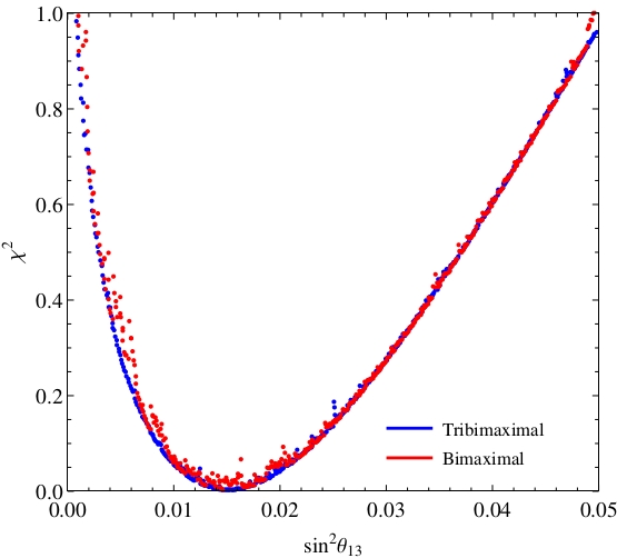
Figure 3: In the $SO(10)$ model the resulting $\chi^{2}$ when starting in the TB or BM basis are equal within errors. Note that the minimum $\chi^{2}$ value, $\chi^{2}=0.003$, is obtained for $\sin^{2}\theta_{13}\sim 0.015$, just a bit below the measured value $\sin^{2}\theta_{13}\sim 0.022$. Nevertheless, as the minimum $\chi^{2}$ is quite shallow for $\sin^{2}\theta_{13}<0.1$, the fit does not exhibit any strongly preferred value of $\theta_{13}$.

A closer look at the details of the fine tuning parameter reveals that high $d_{FT}$ values are predominantly driven by the smallness of the electron mass, combined with its extraordinary measurement precision. Moreover, due to the presence of mixing, the $d_{FT}$ coming from, for instance, the 33 component of $h$, which is mainly responsible for the top mass, is actually one of the largest contributions to the global $d_{FT}$ (due to its contribution to the electron mass) in both TB and BM scenarios. Although this might be surprising at a first glance, we emphasize that the dependence of the observables on the parameters is highly non trivial due to the off-diagonal elements of the mass matrices.

In conclusion, as previously shown in Ref. [28], in this class of $SO(10)$ models one can obtain a reasonable fit to the data. Then one can reinterpret the result as BM corrected by the charged lepton diagonalization and explicitly determine the corrective terms arising from the fit. However the model does not imply BM mixing as a starting approximation. In fact, one could as well focus on TB mixing and make a similar interpretation. To predict, before diagonalization of charged leptons, exact BM in the neutrino sector one would need additional dynamical ingredients. Independent of that, with the present value of $\sin^{2}{\theta_{13}}$, a larger amount of fine tuning is needed in the BM case, as compared to the TB case, in order to reproduce the small values of the first generation masses.

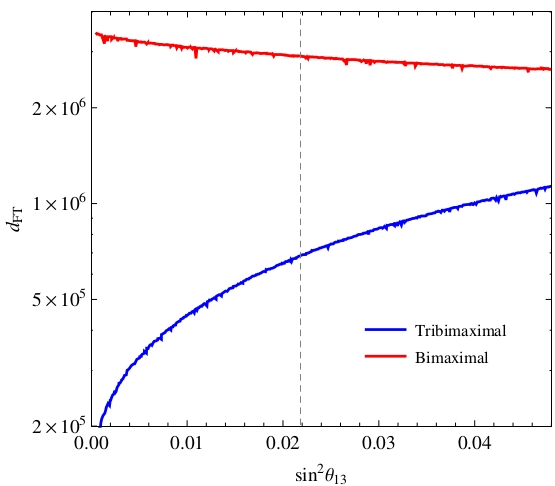
Figure 4: In the $SO(10)$ model the fine tuning parameter $d_{FT}$ increases (decreases) with $\sin^{2}{\theta_{13}}$ in the TB (BM) cases. For the physical value $\sin^{2}{\theta_{13}}\sim 0.022$ it is about 4 times larger in the BM case.

5 Summary and Conclusion

Models of neutrino mixing based on discrete flavour groups have been extensively studied. After the recent measurement of $\sin^{2}{\theta_{13}}$ many of these models have been disfavoured, in particular among those aiming at implementing TB mixing. But models based on $S_{4}$ with BM mixing corrected by terms arising from the diagonalization of the charged lepton mass matrix remain as a viable and attractive possibility. In a GUT context, in these theories, it is also possible to implement the weak form of complementarity i.e. $\theta_{12}+\mathcal{O}(\theta_{C})\sim\pi/4$ and to describe quark and lepton masses and mixings in a all comprehensive approach. Here we have discussed two examples of GUT models of BM, one based on $SU(5)$ and one on $SO(10)$. The $SU(5)$ model discussed here indeed has a broken flavour symmetry that contains $S_{4}$ and imposes the BM structure in the neutrino sector which is then corrected by terms arising from the diagonalization of charged lepton masses. The $SO(10)$ model is based on Type-II see-saw and the origin of BM before diagonalization of charged leptons is in this case left unspecified. We have discussed the phenomenology of these models in the context of the most recent data and their relative merits. We have then compared these models based on a large symmetries with models based on a minimum of symmetry where chance plays a central role, like Anarchy or models based on $U(1)_{FN}$. The $SU(5)$ model with broken $S_{4}$ symmetry emerges as the most viable and predictive theory.

References

- [1] G. Altarelli and F. Feruglio, , Rev. Mod. Phys. 82 2701 (2010) , arXiv:1002.0211.
- [2] H. Ishimori et. al., Prog. Theor. Phys. Suppl. 183, 1 (2010) , arXiv:1003.3552; S. F. King and C. Luhn, arXiv:1301.1340; S. F. King et. al., arXiv:1402.4271.
- [3] W. Grimus and P. O. Ludl, J. Phys. A 45, 233001 (2012) , arXiv:1110.6376.
- [4] L. J. Hall, H. Murayama, and N. Weiner, Phys. Rev. Lett. 84, 2572 (2000) , arXiv:hep-ph/9911341.
- [5] A. de Gouvea and H. Murayama, Phys. Lett. B573, 94 (2003) , arXiv:hep-ph/0301050.
- [6] A. de Gouvea and H. Murayama, arXiv:1204.1249.
- [7] M. C. Gonzalez-Garcia, M. Maltoni and T. Schwetz, JHEP 1411, 052 (2014) [arXiv:1409.5439 [hep-ph]].
- [8] E. Ma and D. Wegman, Phys. Rev. Lett. 107, 061803 (2011) , arXiv:1106.4269; S. F. King and C. Luhn, JHEP 09, 042 (2011) , arXiv:1107.5332; F. Bazzocchi, arXiv:1108.2497; S. Antusch, S. F. King, C. Luhn and M. Spinrath, Nucl. Phys. B 856 (2012) 328 [arXiv:1108.4278 [hep-ph]]; I. de Medeiros Varzielas and L. Merlo, JHEP 02, 062 (2011) , arXiv:1011.6662; F. Bazzocchi and L. Merlo, Fortsch. Phys. 61, 571 (2013) [arXiv:1205.5135 [hep-ph]].
- [9] Y. Lin, Nucl. Phys. B824, 95 (2010) , arXiv:0905.3534.
- [10] See, for example, S. Antusch and S. F. King, New J. Phys. 6 (2004) 110 [hep-ph/0405272].
- [11] R. d. A. Toorop, F. Feruglio and C. Hagedorn, Phys. Lett. B 703 (2011) 447 [arXiv:1107.3486 [hep-ph]]; Nucl. Phys. B858, 437 (2012) , arXiv:1112.1340; S. F. King, C. Luhn and A. J. Stuart, Nucl. Phys. B 867 (2013) 203 [arXiv:1207.5741 [hep-ph]]; C. Hagedorn and D. Meloni, Nucl. Phys. B 862 (2012) 691 [arXiv:1204.0715 [hep-ph]]; M. Holthausen and K. S. Lim, Phys. Rev. D 88 (2013) 033018 [arXiv:1306.4356 [hep-ph]]; S. F. King, T. Neder and A. J. Stuart, Phys. Lett. B 726 (2013) 312 [arXiv:1305.3200 [hep-ph]];
- [12] S. F. Ge, D. A. Dicus and W. W. Repko, Phys. Lett. B 702 (2011) 220 [arXiv:1104.0602 [hep-ph]]; Phys. Rev. Lett. 108 (2012) 041801 [arXiv:1108.0964 [hep-ph]]; D. Hernandez and A. Y. Smirnov, Phys. Rev. D 86 (2012) 053014 [arXiv:1204.0445 [hep-ph]]; Phys. Rev. D 87 (2013) 5, 053005 [arXiv:1212.2149 [hep-ph]].
- [13] G. Ecker, W. Grimus and H. Neufeld, J. Phys. A 20 (1987) L807; Int. J. Mod. Phys. A 3 (1988) 603; W. Grimus and M. N. Rebelo, Phys. Rept. 281 (1997) 239 [hep-ph/9506272]; W. Grimus and L. Lavoura, Phys. Lett. B 579 (2004) 113 [hep-ph/0305309]; R. N. Mohapatra and C. C. Nishi, Phys. Rev. D 86 (2012) 073007 [arXiv:1208.2875 [hep-ph]]; M. Holthausen, M. Lindner and M. A. Schmidt, JHEP 1304 (2013) 122 [arXiv:1211.6953 [hep-ph]]; F. Feruglio, C. Hagedorn and R. Ziegler, JHEP 1307 (2013) 027 [arXiv:1211.5560 [hep-ph]]; Eur. Phys. J. C 74 (2014) 2753 [arXiv:1303.7178 [hep-ph]].
- [14] I. de Medeiros Varzielas and D. Emmanuel-Costa, Phys. Rev. D 84 (2011) 117901 [arXiv:1106.5477 [hep-ph]]; G. Bhattacharyya, I. de Medeiros Varzielas and P. Leser, Phys. Rev. Lett. 109 (2012) 241603 [arXiv:1210.0545 [hep-ph]]; M. C. Chen and K. T. Mahanthappa, Phys. Lett. B 681 (2009) 444 [arXiv:0904.1721 [hep-ph]]; G. J. Ding and S. F. King, Phys. Rev. D 89 (2014) 9, 093020 [arXiv:1403.5846 [hep-ph]]; L. L. Everett, T. Garon and A. J. Stuart, arXiv:1501.04336 [hep-ph]; C. C. Li and G. J. Ding,arXiv:1503.03711 [hep-ph]; A. Di Iura, C. Hagedorn and D. Meloni, arXiv:1503.04140 [hep-ph].
- [15] J. K. Ahn et al. [RENO Collaboration], Phys. Rev. Lett. 108 (2012) 191802 [arXiv:1204.0626 [hep-ex]].
- [16] Y. Abe et al. [Double Chooz Collaboration], Phys. Rev. D 86, 052008 (2012) [arXiv:1207.6632 [hep-ex]].
- [17] F. P. An et al. [Daya Bay Collaboration], Phys. Rev. Lett. 112, 061801 (2014) [arXiv:1310.6732 [hep-ex]].
- [18] K. Abe et al. [T2K Collaboration], Phys. Rev. Lett. 112, 061802 (2014) [arXiv:1311.4750 [hep-ex]].
- [19] V. D. Barger, S. Pakvasa, T. J. Weiler and K. Whisnant, Phys. Lett. B 437, 107 (1998) [hep-ph/9806387].
- [20] R. N. Mohapatra and S. Nussinov, Phys. Rev. D 60, 013002 (1999) [hep-ph/9809415].
- [21] G. Altarelli, F. Feruglio and L. Merlo, JHEP 0905, 020 (2009) [arXiv:0903.1940 [hep-ph]].
- [22] D. Meloni, JHEP 1110 (2011) 010 [arXiv:1107.0221 [hep-ph]].
- [23] M. Raidal, Phys. Rev. Lett. 93, 161801 (2004) [hep-ph/0404046].
- [24] H. Minakata and A. Y. Smirnov, Phys. Rev. D 70, 073009 (2004) [hep-ph/0405088].
- [25] P. H. Frampton and R. N. Mohapatra, JHEP 0501, 025 (2005) [hep-ph/0407139].
- [26] S. Antusch, S. F. King and R. N. Mohapatra, Phys. Lett. B 618, 150 (2005) [hep-ph/0504007].
- [27] K. M. Patel, Phys. Lett. B 695, 225 (2011) [arXiv:1008.5061 [hep-ph]].
- [28] G. Altarelli and G. Blankenburg, JHEP 1103 (2011) 133 [arXiv:1012.2697 [hep-ph]].
- [29] C. D. Froggatt and H. B. Nielsen, Nucl. Phys. B 147 (1979) 277.
- [30] G. Altarelli, F. Feruglio, I. Masina and L. Merlo, JHEP 1211 (2012) 139 [arXiv:1207.0587 [hep-ph]].
- [31] J. Bergstrom, D. Meloni and L. Merlo, Phys. Rev. D 89 (2014) 9, 093021 [arXiv:1403.4528 [hep-ph]].
- [32] E. Witten, Nucl. Phys. B 258 (1985) 75; Y. Kawamura, Prog. Theor. Phys. 105 (2001) 999 [arXiv:hep-ph/0012125]; A. E. Faraggi, Phys. Lett. B 520 (2001) 337 [arXiv:hep-ph/0107094] and references therein.
- [33] L. J. Hall and Y. Nomura, Phys. Rev. D 64 (2001) 055003 [arXiv:hep-ph/0103125]; Y. Nomura, Phys. Rev. D 65 (2002) 085036 [arXiv:hep-ph/0108170]; L. J. Hall and Y. Nomura, Phys. Rev. D 66 (2002) 075004 [arXiv:hep-ph/0205067].
- [34] G. Altarelli and F. Feruglio, Phys. Lett. B 511 (2001) 257 [arXiv:hep-ph/0102301]; A. Hebecker and J. March-Russell, Nucl. Phys. B 613 (2001) 3 [arXiv:hep-ph/0106166]; A. Hebecker and J. March-Russell, Phys. Lett. B 541 (2002) 338 [arXiv:hep-ph/0205143].
- [35] G. Altarelli, F. Feruglio, C. Hagedorn, JHEP 0803, 052-052 (2008). [arXiv:0802.0090 [hep-ph]].
- [36] A. S. Joshipura and K. M. Patel, Phys. Rev. D 83, 095002 (2011) [arXiv:1102.5148 [hep-ph]].
- [37] G. Altarelli, F. Feruglio and I. Masina, JHEP 0301 (2003) 035 [hep-ph/0210342].
- [38] G. Altarelli, F. Feruglio, I. Masina and L. Merlo, JHEP 1211 (2012) 139 [arXiv:1207.0587 [hep-ph]].
- [39] G. Lazarides, Q. Shafi and C. Wetterich, Nucl. Phys. B 181, 287 (1981); J. Schechter and J. W. F. Valle, Phys. Rev. D 22, 2227 (1980); R. N. Mohapatra and G. Senjanovic, Phys. Rev. D 23, 165 (1981).
- [40] P. Minkowski, Phys. Lett. B 67 (1977) 421; T. Yanagida in Workshop on Unified Theories, KEK Report 79-18, p. 95, 1979; M. Gell-Mann, P. Ramond and R. Slansky, Supergravity, p. 315, Amsterdam: North Holland, 1979; S. L. Glashow, 1979 Cargese Summer Institute on Quarks and Leptons, p. 687, New York: Plenum, 1980; R. N. Mohapatra and G. Senjanovic, Phys. Rev. Lett, 44 (1980) 912.
- [41] B. Dutta, Y. Mimura and R. N. Mohapatra, Phys. Rev. Lett. 94, 091804 (2005) [hep-ph/0412105], Phys. Rev. D 72, 075009 (2005) [hep-ph/0507319], Phys. Rev. D80 (2009) 095021 [ArXiv:0910.1043 [hep-ph]].
- [42] H. S. Goh, R. N. Mohapatra and S. P. Ng, Phys. Lett. B 570, 215 (2003) [hep-ph/0303055], Phys. Rev. D 68, 115008 (2003) [hep-ph/0308197]; H. S. Goh, R. N. Mohapatra and S. Nasri, Phys. Rev. D70 075022 (2004) [hep-ph/0408139].
- [43] C. S. Aulakh, B. Bajc, A. Melfo, G. Senjanovic and F. Vissani, Phys. Lett. B 588, 196 (2004) [hep-ph/0306242].
- [44] C. S. Aulakh and S.K Garg, Nucl. Phys. B757 47 (2006) [hep-ph/0512224], [hep-ph/0612021].
- [45] B. Bajc, A. Melfo, G. Senjanovic, F. Vissani, Phys. Lett. B634 (2006)272 [ArXiv:0511352 [hep-ph]].
- [46] A. Melfo, A. Ramirez and G. Senjanovic, Phys. Rev. D82 (2010) 075014 [ArXiv:1005.0834 [hep-ph]].