Tunable thermoelectricity in monolayers of MoS₂ and other group-VI dichalcogenides

Abstract

We study the thermoelectric properties of monolayers of MoS₂ and other group-VI dichalcogenides under circularly polarized off-resonant light. Analytical expressions are derived for the Berry phase mediated magnetic moment, orbital magnetization, as well as thermal and Nernst conductivities. Tuning of the band gap by off-resonant light enhances the spin splitting in both the valence and conduction bands and, thus, leads to a dramatic improvement of the spin and valley thermoelectric properties.

I Introduction

Being the first truly two dimensional material 1 , graphene has attracted remarkable attention, both due to its exotic transport behavior and technological applications in various fields 2 . Still, fundamental problems restrict its applicability, in particular the negligible band gap and weak spin orbit coupling (SOC). These limitations could be overcome by monolayer MoS₂, which therefore is interesting for next generation nanoelectronics 3 ; 4 ; 5 ; 6 ; 7 . MoS₂ combines the honeycomb structure of graphene with a large intrinsic direct band gap of $2\Delta=1.66$ eV and a large SOC of $\lambda=74$ meV, providing mass to the Dirac fermions 8 ; 9 ; 10 . As a consequence, preliminary results indicate potential in valleytronics, because the dispersion can be manipulated in a flexible manner for optoelectronic applications 10 ; 11 ; 12 ; 13 . Spin and valley Hall effects have been predicted in an experimentally accessible temperature regime 9 , the former arising from the strong SOC and the latter from the broken inversion symmetry.

In addition to the electrical and optical properties, Berry phase mediated thermoelectric effects due to a temperature gradient have been proposed for two-dimensional systems 15 . Orbital magnetic moments, orbital magnetizations 17 , as well as thermal and Nernst conductivities have been addressed in Refs. 19 ; 20 ; 21 and theoretical models for the thermoelectric transport have been presented for graphene in Ref. 22 and for topological insulators in Ref. 23 . Of particular interest is the tuning of the spin and valley thermoelectric properties of MoS₂ and other group-VI dichalcogenides, where a temperature gradient gives rise to transverse spin/valley accumulation and spin/valley current. In graphene this is difficult to realize due to the negligible band gap and weak SOC.

In the present work we quantify the Berry phase mediated thermoelectric properties of MoS₂ and other group-VI dichalcogenides by deriving analytical expressions for the key thermoelectric quantities in the presence of circularly polarized off-resonant light. Gap opening by such light has been predicted for graphene and for the surface states of topological insulators 24 , and has been confirmed experimentally for the latter 25 . For graphene the chiralities for different values of the frequency have been given in Ref. new1 . Moreover, opening of a trivial gap has been reported under high-frequency linearly polarized light new2 . Going beyond these findings, we demonstrate in the following that by off-resonant light large spin and valley thermoelectric effects can be achieved.

II Model formulation

Extending the approach of Ref. 9 by introducing time dependence, we start from the effective Hamiltonian

$$H^{s_{z},\eta}(t)=v(\eta\sigma_{x}\Pi_{x}(t)+\sigma_{y}\Pi_{y}(t))+\Delta\sigma_{z}-\lambda\eta s_{z}\sigma_{z}+\lambda\eta s_{z}{\bf I}$$ (1)

in the $xy$-plane in the presence of circularly polarized light, where $\eta=\pm 1$ represents the $K$- and $K^{\prime}$-valleys, respectively, $\Delta$ is the mass term that breaks the inversion symmetry, $\sigma_{x}$, $\sigma_{y}$, and $\sigma_{z}$ are the Pauli matrices, $\lambda$ is the SOC with real spin index $s_{z}$, and $v=at_{0}/\hbar$ is the Fermi velocity of the Dirac fermions (with $t_{0}$ being the nearest neighbour hopping amplitude and $a$ the lattice constant). We use the gauge in the two-dimensional canonical momentum $\mathbf{\Pi(}t\mathbf{)=p}+e\mathbf{A(}t\mathbf{)}$ with vector potential

$$\mathbf{A}(t)=(\pm A\sin\Omega t,A\cos\Omega t),$$ (2)

where $\Omega$ is the frequency of the light and $A=E_{0}/\Omega$ ($E_{0}$ is the amplitude of the electric field, $\mathbf{E}(t)=-\partial\mathbf{A}(t)/\partial t$). We have $\mathbf{A}(t+T_{0})=\mathbf{A}(t)$ for $T_{0}=2\pi/\Omega$. The plus/minus sign in Eq. (2) refers to right/left-handed circular polarization of the light.

The effect of off-resonant light can be described by a static Floquet Hamiltonian 24 , which yields excellent agreement with experiments 25 . A static approach is satisfied for low intensity ($evA\ll\hslash\Omega$) and high frequency ($t_{0}\ll\hslash\Omega$) light, which does not directly excite electrons but effectively modifies the band structure through virtual photon absorption and emission processes. We arrive at the effective Hamiltonian (see the Appendix)

$$H_{eff}^{s_{z},\eta}=v(\eta\sigma_{x}p_{x}+\sigma_{y}p_{y})+(\Delta+\eta\Delta_{\Omega})\sigma_{z}-\lambda\eta s_{z}\sigma_{z}+\lambda\eta s_{z}{\bf I},$$ (3)

where $\Delta_{\Omega}=e^{2}v^{2}\hslash^{2}A^{2}/\hslash^{3}\Omega^{3}$ is an effective energy term representing the circularly polarized off-resonant light, which essentially renormalizes the mass of the Dirac fermions. Similar approaches have been used for describing gapped systems such as silicene 26 and disordered topological insulators 27 . Diagonalization of the Hamiltonian leads to the eigenvalues

$$E_{\zeta}^{s,\eta}=s\eta\lambda+\zeta\sqrt{(v\hslash k)^{2}+(\Delta+\eta\Delta_{\Omega}-\lambda\eta s)^{2}}$$ (4)

and eigenfunctions

$$\Psi_{\zeta}^{s,\eta}(\mathbf{k})=\frac{e^{ik_{x}x+ik_{y}y}}{\sqrt{L_{x}L_{y}}}\left(\begin{array}[]{c}\frac{v\hslash ke^{-i\eta\varphi}}{\sqrt{(v\hslash k)^{2}+\left[-\Delta-\eta\Delta_{\Omega}+\eta s\lambda+\zeta\sqrt{(v\hslash k)^{2}+(\Delta+\Delta_{\Omega}-\lambda\eta s)^{2}}\right]^{2}}}\\ \frac{-\Delta-\eta\Delta_{\Omega}+\eta s\lambda+\zeta\sqrt{(v\hslash k)^{2}+(\Delta+\Delta_{\Omega}-\lambda\eta s)^{2}}}{\sqrt{(v\hslash k)^{2}+\left[-\Delta-\eta\Delta_{\Omega}+\eta s\lambda+\zeta\sqrt{(v\hslash k)^{2}+(\Delta+\Delta_{\Omega}-\lambda\eta s)^{2}}\right]^{2}}}\end{array}\right).$$ (5)

Here $\zeta=\pm 1$ denotes electron/hole bands, $s$ = $\pm$1 stands for spin up/down, and $\varphi=\tan^{-1}(k_{y}/k_{x})$ with $k_{x}=k\cos\varphi$, $k_{y}=k\sin\varphi$, and $k=\sqrt{k_{x}^{2}+k_{y}^{2}}$.

The energy eigenvalues $E_{\zeta}^{s,\eta}$ are illustrated in Fig. 1. For $\hslash\Omega=10t_{0}=11$ eV the circularly polarized light is in the off-resonance regime, where $\Delta_{\Omega}=0.6$ eV ($evA=2.58$ eV, top row of Fig. 1) or $\Delta_{\Omega}=0.8$ eV ($evA=2.97$ eV, bottom row of Fig. 1). The direct band gap of MoS₂ amounts to $\Delta=0.83$ eV and we have $\lambda=37$ meV, $v=0.5\times$10⁵ m/s, and $a=3.193$ Å 9 . For $\Delta_{\Omega}=0.6$ eV the band gap is reduced to 0.46 eV for the $K^{\prime}$-valley (top right) and enlarged to 2.86 eV for the $K$-valley (top left). The effect of the off-resonant light ($\Delta_{\Omega}$) can be tuned by varying the intensity, where various values have been achieved experimentally 25 . For $\Delta_{\Omega}=0.8$ eV we observe that the spin splitting in the conduction band is increased and the band gap is reduced to 0.06 eV in the $K^{\prime}$-valley, so that only the $K^{\prime}$-valley is relevant, whereas for the $K$-valley the band gap becomes 3.26 eV. In the following we restrict the discussion to the $K^{\prime}$-valley ($\eta=-1$).

III Orbital magnetic moment and temperature dependent orbital magnetization

In order to study the Berry phase mediated thermoelectric transport, we consider the free energy, which, for a weak magnetic field $\mathbf{B}$, is given by 15

$$F_{\zeta}^{s,-1}=-\frac{1}{\beta}\sum_{\mathbf{k}}\log\left(1+e^{-\beta(E_{\zeta}^{s,-1}(\mathbf{k})-\mu)}\right),$$ (6)

where $\beta=1/k_{B}T$, $k_{B}=8.62\times 10^{-5}$ eV/K is the Boltzmann constant, $\mu$ is the Fermi energy, and $T$ is the temperature. Eq. (6) can be simplified by converting the summation into an integral,

$$F_{\zeta}^{s,-1}=-\frac{1}{\beta}\int\frac{d^{2}k}{(2\pi)^{2}}\left(1+\frac{e}{\hslash}\mathbf{\Omega}_{\zeta}^{s,-1}(\mathbf{k})\cdot\mathbf{B}\right)\log\left(1+e^{-\beta(E_{\zeta}^{s,-1}(\mathbf{k})-\mu)}\right),$$ (7)

where

$$\mathbf{\Omega}_{\zeta}^{s,-1}(\mathbf{k})=\mathbf{\nabla}_{\mathbf{k}}\times\left\langle\Psi_{\zeta}^{s,-1}(\mathbf{k})\left|i\mathbf{\nabla}_{\mathbf{k}}\right|\Psi_{\zeta}^{s,-1}(\mathbf{k})\right\rangle\mathbf{\hat{z}}$$ (8)

is the Berry curvature. The energy $E_{\zeta}^{s,-1}(\mathbf{k})=E_{\zeta}^{s,-1}-\mathbf{m}_{\zeta}^{s,-1}\mathbf{(k)}\cdot\mathbf{B}$ is modified by the orbital magnetic moment

$$\mathbf{m}_{\zeta}^{s,-1}(\mathbf{k})=\frac{-ie}{\hslash}\left\langle\nabla_{\mathbf{k}}\Psi_{\zeta}^{s,-1}(\mathbf{k})\left|\hat{H}-E_{\zeta}^{s,-1}\right|\nabla_{\mathbf{k}}\Psi_{\zeta}^{s,-1}(\mathbf{k})\right\rangle\mathbf{\hat{z}.}$$ (9)

The orbital magnetization then is obtained as

$$\mathbf{M}_{\zeta}^{s,-1} = -\left(\frac{\partial F_{\zeta}^{s,-1}}{\partial\mathbf{B}}\right)_{\mu,T}$$

$$= \int\frac{d^{2}k}{(2\pi)^{2}}f(E_{\zeta}^{s,-1}(\mathbf{k}))\mathbf{m}_{\zeta}^{s,-1}\mathbf{(k)}+\frac{e}{\beta\hslash}\int\frac{d^{2}k}{(2\pi)^{2}}\mathbf{\Omega}_{\zeta}^{s,-1}\mathbf{(k)}\log\left(1+e^{-\beta(E_{\zeta}^{s,-1}(\mathbf{k})-\mu)}\right),$$

where $f$ is the Fermi distribution function. From Eqs. (4) and (5) we obtain for the $z$-component of the Berry curvature

$$\Omega_{\zeta}^{s,-1}(\mathbf{k})=\frac{\hslash^{2}v^{2}}{2}\frac{\Delta-\Delta_{\Omega}+s\lambda}{\left[(v\hslash k)^{2}+(\Delta-\Delta_{\Omega}+s\lambda)^{2}\right]^{3/2}}$$ (11)

and correspondingly for the $z$-component of the orbital magnetic moment

$$m_{\zeta}^{s,-1}(\mathbf{k})=\frac{e}{\hslash}E_{\zeta}^{s,-1}\Omega_{\zeta}^{s,-1}(\mathbf{k}).$$ (12)

For finite $\Delta-\Delta_{\Omega}+s\lambda$ the orbital magnetic moment has a peak at $k=0$. For $\lambda=0$ we obtain for $\Delta-\Delta_{\Omega}$ = 30 meV for a single valley and $\Delta_{\Omega}=0.8$ eV an orbital magnetic moment of 35 Bohr magnetons. High magnetic moments have been predicted for systems involving orbital degrees of freedom, such as graphene 17 .

Using Eqs. (11) and (12) in Eq. (10), we obtain for $T\rightarrow 0$ for the conduction band the $z$-component

$$M_{+1}^{s,-1}=\frac{e\mu}{2h}\left(1-\frac{\Delta-\Delta_{\Omega}+s\lambda}{\mu+s\lambda}\right),$$ (13)

which again can be enhanced by reducing the band gap by off-resonant light. Eq. (13) reduces to a previous result for gapped graphene in Ref. 17 in the limit of $\lambda=0$ and $\Delta_{\Omega}=0$. As an example, for $\mu$ = 0.2 eV we obtain an orbital magnetization (by dividing the results of Eq. (13) by a typical layer thickness of 0.6 nm) of 0.1 Tesla, which is well detectable in experiments.

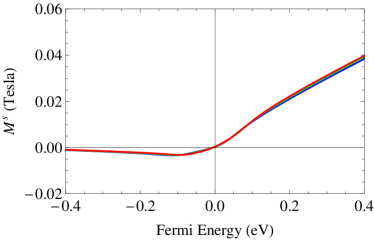
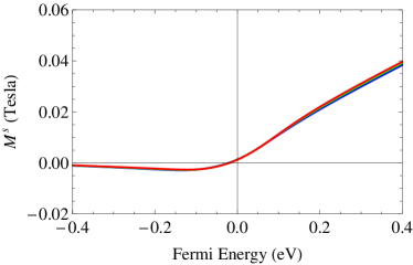
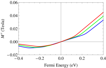
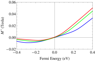
Figure 2: Spin (top) and valley (bottom) orbital magnetizations (divided by the layer thickness 0.6 nm) as a function of the Fermi energy for $T$ = 160 K (left) and $T$ = 360 K (right). For $M^{s}$ we use $\Delta_{\Omega}=0.8$ eV (blue), $\Delta_{\Omega}=0.81$ eV (green), and $\Delta_{\Omega}=0.82$ eV (red), whereas for $M^{v}$ we use $\Delta_{\Omega}=0.6$ eV (blue), $\Delta_{\Omega}=0.65$ eV (green), and $\Delta_{\Omega}=0.7$ eV (red). All other parameters are the same as in Fig. 1.

In order to evaluate temperature effects, we study the spin and valley orbital magnetizations $M^{s}=M_{\zeta}^{+1,-1}-M_{\zeta}^{-1,-1}$ and $M^{v}=M_{\zeta}^{+1,-1}+M_{\zeta}^{-1,-1}$, using Eq. (8), in Fig. 2 as a function of the Fermi energy for temperatures of $T$ = 160 K (left) and $T$ = 360 K (right). To achieve spin and valley orbital magnetizations, respectively, we require $\lambda>\left|\Delta-\Delta_{\Omega}\right|$ and $\lambda<\left|\Delta-\Delta_{\Omega}\right|$. $M^{v}$ is growing faster in the conduction band than in the valence band and is much/slightly larger than $M^{s}$ in the valence/conduction band. Increasing the intensity of the off-resonant light increases/decreases $M^{v}$ in the conduction/valence band due to a slow/fast reduction of the band gap, which is due to the energy shift by SOC (see Eq. (4)).

As compared to Fig. 2, without off-resonant light we obtain about half the value for $M^{v}$, while $M^{s}$ is 100 times smaller (with opposite sign), since it is dominated by the band gap (the system is pinned to the valley transport regime). For $T=160$ K we observe spin effects close to the Dirac point, whereas they are suppressed for $T=360$ K. These effects will become clear in the next section, since the orbital magnetization is proportional to the Hall conductivity 17 . Susceptibility measurements, electron paramagnetic resonance, x-ray magnetic circular dichroism, and neutron diffraction can be used to probe the orbital magnetization 30 ; 31 ; 32 .

IV Spin/valley thermal and Nernst Conductivities

Eq. (10) contains conventional (first term) and Berry phase mediated (second term) contributions. It has been demonstrated in Refs. 15 ; 17 that the conventional part does not contribute to the transport, while the Berry term directly modifies the intrinsic Hall current (which is obtained by integrating the Berry curvature over the two-dimensional Brillouin zone). In contrast to the Hall conductivity, the Nernst conductivity is determined not only by the Berry curvature but also by entropy generation around the Fermi surface 22 ; 23 and therefore is sensitive to changes of the Fermi energy and temperature. For a weak electric field $\mathbf{E}$, the Hall current is given by $j_{x}=\alpha_{xy}^{s,-1}(-\nabla_{y}T)$ and the Nernst conductivity by 22

$$\alpha_{xy}^{s,-1}=\frac{ek_{B}}{\hslash}\sum_{\mathbf{s,\zeta}}\int\frac{d^{2}k}{(2\pi)^{2}}\Omega_{\zeta}^{s,-1}(\mathbf{k})S_{\zeta}^{s,-1}(\mathbf{k}),$$ (14)

$S_{\zeta}^{s,-1}(\mathbf{k})=-f(E_{\zeta}^{s,-1}(\mathbf{k})-\mu)\ln f(E_{\zeta}^{s,-1}(\mathbf{k})-\mu)-\left(1-f(E_{\zeta}^{s,-1}(\mathbf{k})-\mu)\right)\ln\left(1-f(E_{\zeta}^{s,-1}(\mathbf{k})-\mu)\right)$ being the entropy density. Recent experiments found that Eq. (14) describes graphene very well 33 . We obtain the transverse thermal conductivity

$$\kappa_{xy}^{s,-1} = \frac{k_{B}e}{\beta h}\sum_{\mathbf{s,\zeta}}\int\frac{d^{2}k}{(2\pi)^{2}}\Omega_{\zeta}^{s,-1}(\mathbf{k})\left\{\frac{\pi^{2}}{3}+\beta^{2}(E_{\zeta}^{s,-1}(\mathbf{k})-\mu)^{2}f(E_{\zeta}^{s,-1}(\mathbf{k})-\mu)\right.$$

$$\left.-\ln^{2}\left(1+e^{-\beta(E_{\zeta}^{s,-1}(\mathbf{k})-\mu)}\right)-2\text{Li}_{2}\left(1-f(E_{\zeta}^{s,-1}(\mathbf{k})-\mu)\right)\right\},$$

where Li₂ is the polylogarithm. Eqs. (14) and (15) can be simplified in the limit of low temperature, using Mott relations 15 , to

$$\alpha_{xy}^{s,-1}=-\frac{\pi^{2}}{3}\frac{k_{B}^{2}}{e}T\frac{d\sigma_{xy}^{s,-1}}{d\mu}=-e\frac{d\kappa_{xy}^{s,-1}}{d\mu}$$ (16)

and

$$\kappa_{xy}^{s,-1}=\frac{\pi^{2}}{3}\frac{k_{B}^{2}}{e^{2}}T\sigma_{xy}^{s,-1},$$ (17)

where

$$\sigma_{xy}^{s,-1}=\frac{e^{2}}{\hslash}\int\frac{d^{2}k}{(2\pi)^{2}}\left(f_{+}(E)-f_{-}(E)\right)\Omega_{\zeta}^{s,-1}(\mathbf{k})$$ (18)

with $f_{\pm}$ representing the distribution function of the electron/hole bands. According to Eq. (16), the Nernst conductivity is proportional to the derivative of the thermal conductivity. We solve Eq. (18) for $T=0$ by performing the integral and obtain in the case that the Fermi level is in the conduction band

$$\sigma_{xy}^{s,-1}=-\frac{e^{2}}{2h}\frac{\Delta-\Delta_{\Omega}+s\lambda}{\mu+s\lambda}.$$ (19)

Eqs. (14) and (19) show that the spin ($\alpha_{xy}^{s}=\alpha_{xy}^{+1,-1}-\alpha_{xy}^{-1,-1}$) and valley ($\alpha_{xy}^{v}=\alpha_{xy}^{+1,-1}+\alpha_{xy}^{-1,-1}$) Nernst conductivities are enhanced under off-resonant light. Without off-resonant light the spin Nernst conductivity is negligible because of the vanishing spin Hall conductivity in the limit $\Delta\gg\lambda$ (the system is pinned to the valley Hall regime). Due to the large band gap, the valley Nernst conductivity is also small for $t_{0}<\Delta$. An enhanced spin splitting and corresponding giant thermoelectric transport in both the conduction and valence bands is achieved by reducing the band gap (to the range of $\lambda$). The results in Eqs. (14) and (19) guarantee for monolayers of MoS₂ and related group-VI dichalcogenides an electrically tunable band gap to tailor the spin and valley transport.

Experiments indicate that the thermoelectric properties can be understood by Mott relations, which agree with experimental data for low temperature 33 ; 34 ; 35 ; 36 . In these experiments the thermoelectric properties, in particular the Nernst conductivity, have been measured for gapless graphene in a transverse magnetic field. The Nernst effect discussed in our work exists even without external magnetic field, being solely driven by the effective magnetic field due to the Berry curvature. Note that Eq. (14) is more general than Eq. (16), because it goes beyond the linear temperature dependence.

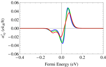
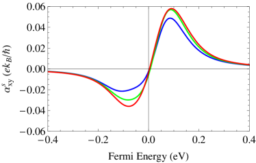
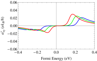
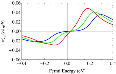
Figure 3: Spin (top) and valley (bottom) Nernst conductivities as a function of the Fermi energy for $T$ = 160 K (left) and $T$ = 360 K (right). For $\alpha_{xy}^{s}$ we use $\Delta_{\Omega}=0.8$ eV (blue), $\Delta_{\Omega}=0.81$ eV (green), and $\Delta_{\Omega}=0.82$ eV (red), whereas for $\alpha_{xy}^{v}$ we use $\Delta_{\Omega}=0.6$ eV (blue), $\Delta_{\Omega}=0.65$ eV (green), and $\Delta_{\Omega}=0.7$ eV (red). All other parameters are the same as in Fig. 1.

It has been found experimentally that the dependence of the thermoelectric transport on the gate voltage (Fermi energy) can be tuned by controlling the band gap in monolayer 19 ; 20 ; 21 ; 33 ; 34 ; 35 and bilayer 36 graphene. Being the electrical response to the thermodynamic perturbation, a giant thermoelectric transport is achieved when the bands come close to the Dirac point. In Fig. 3 (top) we show numerical results for $\alpha_{xy}^{s}$, by evaluating Eq. (14), as function of the Fermi energy at $T=160$ K (left) and $T=360$ K (right) and vary the band gap by off-resonant light as $\Delta_{\Omega}=0.8$ eV (blue), $\Delta_{\Omega}=0.81$ eV (green), and $\Delta_{\Omega}=0.82$ eV (red). For $T=160$ K we find two peaks with negative values, where the lower peak is a consequence of the spin splitting and is washed out for $T=360$ K. Our results show that a significant spin dependent transport can be observed in MoS₂ and related group-VI dichalcogenides at room temperature (or even above). Figure 3 (bottom) shows $\alpha_{xy}^{v}$ as a function of the Fermi energy for $T=160$ K (left) and $T=360$ K (right) with $\Delta_{\Omega}=0.6$ eV (blue), $\Delta_{\Omega}=0.65$ eV (green), and $\Delta_{\Omega}=0.7$ eV (red). We observe shifts of the peaks towards the Dirac point for increasing $\Delta_{\Omega}$, which reflects the reduction of the band gap. The amplitude grows for decreasing band gap. For $\Delta_{\Omega}=0.8$ to 0.82 eV $\alpha_{xy}^{s}$ is enhanced, whereas below $\Delta_{\Omega}=0.793$ eV we are in the valley transport regime and obtain an enhancement of $\alpha_{xy}^{v}$. The transport is huge as compared to the case without off-resonant light.

In general, it depends on the sign of the Berry curvature (compare Fig. 1) whether the Nernst conductivity is positive or negative. Our results are valid for elevated temperature in the experimentally relevant range 33 . Furthermore, $\alpha_{xy}^{s,-1}$ $\neq 0$ when the Fermi energy is in the band gap, whereas Eq. (16) yields $\alpha_{xy}^{s,-1}=0$ (being the derivative of $\sigma_{xy}^{s,-1}$, which is quantized and independent of $\mu$ in this case). The demonstrated enhancement of the spin/valley transport due to the tunability of the band gap in MoS₂ and other group-VI dichalcogenides has been desired for thermoelectric applications since the discovery of graphene. Band gap opening by off-resonant light has been achieved in Ref. 25 for the surface states of topological insulators and can also be used for monolayer MoS₂, since transistors 5 and amplifiers 6 already have been realized.

V Conclusion

We have derived analytical results for the thermoelectric transport in monolayer MoS₂ and related group-VI dichalcogenides in the presence of off-resonant light. We have shown that an increased intensity of the light reduces the direct band gap and results in a strong spin splitting in the conduction band and, therefore, in dramatic enhancement of the thermoelectric transport. The spin splitting in the conduction band (in contrast to the valence band) is negligible without external perturbation (such as off-resonant light). The band gap even can be tuned to zero with giant spin splitting in both the valence and conduction bands. The enhancement of the spin/valley transport properties demonstrated here is desired for spin/valley dependent thermoelectric devices, whereas the tunable band gap opens new directions for fundamental transport experiments.

Appendix A

The time dependence in Eq. (1) can be understood as the sum of two second-order virtual photon processes, where electrons absorb and then emit a photon and electrons emit and then absorb a photon 24 . Within Floquet theory, we use the fact that

$$H_{eff}^{s_{z},\eta}=\frac{i}{T_{0}}\log[U(T_{0})]$$ (A.1)

with

$$U(T_{0})=\text{\^{T}}\exp\left[-i\int_{0}^{T_{0}}H^{s_{z},\eta}(t)dt\right]\simeq\exp[-iH_{eff}^{s_{z},\eta}T_{0}],$$ (A.2)

where T̂ is the time ordering operator. We consider the Fourier decomposition

$$H^{s_{z},\eta}(t)=\sum_{n=-\infty}^{\infty}H_{n}^{s_{z},\eta}e^{in\Omega t}\simeq H_{0}^{s_{z},\eta}+H_{1}^{s_{z},\eta}e^{i\Omega t}+H_{-1}^{s_{z},\eta}e^{-i\Omega t},$$ (A.3)

where we have used

$$H_{n}^{s_{z},\eta}=\frac{1}{T_{0}}\int_{0}^{T_{0}}e^{-{\rm sgn}(n)i\Omega t}H^{s_{z},\eta}(t)dt.$$ (A.4)

Expanding the exponential function in Eq. (A.2) in a Taylor series yields

$$\exp\left[-i\int_{0}^{T_{0}}H^{s_{z},\eta}(t)dt\right]=1-i\int_{0}^{T_{0}}H^{s_{z},\eta}(t)dt+\frac{(-i)^{2}}{2}\int_{0}^{T_{0}}H^{s_{z},\eta}(t_{1})dt_{1}\int_{0}^{T_{0}}H^{s_{z},\eta}(t_{2})dt_{2}+...$$ (A.5)

and thus

$$U(T_{0})\simeq\text{\^{T}}\left(1-i\int_{0}^{T_{0}}H^{s_{z},\eta}(t)dt+\frac{(-i)^{2}}{2}\int_{0}^{T_{0}}H^{s_{z},\eta}(t_{1})dt_{1}\int_{0}^{T_{0}}H^{s_{z},\eta}(t_{2})dt_{2}\right).$$ (A.6)

By applying the time ordering operator in Eq. (A.6) we arrive at

$$U(T_{0}) \simeq 1-i\int_{0}^{T_{0}}H^{s_{z},\eta}(t)dt-\frac{1}{2}\int_{0}^{T_{0}}dt_{1}\int_{0}^{T_{1}}dt_{2}H^{s_{z},\eta}(t_{1})H^{s_{z},\eta}(t_{2})$$

$$-\frac{1}{2}\int_{0}^{T_{0}}dt_{2}\int_{0}^{T_{2}}dt_{1}H^{s_{z},\eta}(t_{2})H^{s_{z},\eta}(t_{1}).$$

Executing the integration in Eq. (A.7) with the help of Eq. (A.3) and reordering the terms, we obtain

$$U(T_{0}) \simeq 1-iH_{0}^{s_{z},\eta}T_{0}-\frac{T_{0}}{\Omega}\left(\pi(H_{0}^{s_{z},\eta})^{2}-i([H_{0}^{s_{z},\eta},H_{-1}^{s_{z},\eta}]-[H_{0}^{s_{z},\eta},H_{1}^{s_{z},\eta}]+[H_{-1}^{s_{z},\eta},H_{1}^{s_{z},\eta}])\right)$$ (A.8)

$$=1-iH_{eff}^{s_{z},\eta}T_{0}-\frac{1}{2}(H_{eff}^{s_{z},\eta}{})^{2}T_{0}^{2}+...$$

and thus

$$H_{eff}^{s_{z},\eta}=H_{0}^{s_{z},\eta}+\frac{1}{\hslash\Omega}\left([H_{0}^{s_{z},\eta},H_{+1}^{s_{z},\eta}]-[H_{0}^{s_{z},\eta},H_{-1}^{s_{z},\eta}]\right)+\frac{1}{\hslash\Omega}[H_{+1}^{s_{z},\eta},H_{-1}^{s_{z},\eta}]$$ (A.9)

with $H_{0}^{s_{z},\eta}=$ $v(\eta\sigma_{x}p_{x}+\sigma_{y}p_{y})+\Delta\sigma_{z}-\lambda\eta s_{z}\sigma_{z}+\lambda\eta s_{z}$, which describes a static honeycomb lattice with hopping $t_{0}$ (in a standard tight binding notation) and a band gap of 2$\Delta$. When $\hslash\Omega\gg t_{0}$ and $\Delta$ then the off-resonance condition is satisfied and perturbation theory can be applied. Since the first order term in Eq. (A.9) vanishes, we simplify the second order term to arrive at the effective Hamiltonian of Eq. (3).

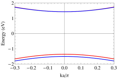
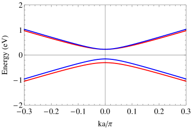
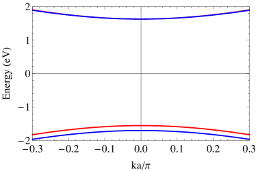
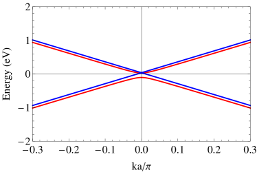
Figure 1: Band structure of monolayer MoS₂ in the presence of off-resonant light and SOC for the $K$-valley (left) and $K^{\prime}$-valley (right) using $\hslash\Omega=10t_{0}$ = 11 eV, $\Delta$ = 0.83 eV, $\lambda=37$ meV, $v=0.5\times$10⁵ m/s, and $a=3.193$ Å. The top row refers to $\Delta_{\Omega}=0.6$ eV and the bottom row to $\Delta_{\Omega}=0.8$ eV.

- (1) A. H. Castro Neto, F. Guinea, N. M. R. Peres, K. S. Novoselov, and A. K. Geim, Rev. Mod. Phys. 81, 109 (2009).
- (2) C. Lee, Q. Li, W. Kalb, X. Z. Liu, H. Berger, R.W. Carpick, and J. Hone, Science 328, 76 (2010).
- (3) A. Splendiani, L. Sun, Y. Zhang, T. Li, J. Kim, C. Y. Chim, G. Galli, and F. Wang, Nano Lett. 10, 1271 (2010).
- (4) K. F. Mak, C. Lee, J. Hone, J. Shan, and T. F. Heinz, Phys. Rev. Lett. 105, 136805 (2010).
- (5) B. Radisavljevic, A. Radenovic, J. Brivio, V. Giacometti, and A. Kis, Nat. Nanotech. 6, 147 (2011).
- (6) T. Korn, S. Heydrich, M. Hirmer, J. Schmutzler, and C. Schüller, Appl. Phys. Lett. 99, 102109 (2011).
- (7) B. Radisavljevic, M. B. Whitwick, and A. Kis, Appl. Phys. Lett. 101, 043103 (2012).
- (8) Z. Y. Zhu, Y. C. Cheng, and U. Schwingenschlögl, Phys. Rev. B 84, 153402 (2011).
- (9) D. Xiao, G.-B. Liu, W. Feng, X. Xu, and W. Yao, Phys. Rev. Lett. 108, 196802 (2012).
- (10) T. Cao, G. Wang, W. Han, H. Ye, C. Zhu, J. Shi, Q. Niu, P. Tan, E. Wang, B. Liu, and J. Feng, Nat. Commun. 3, 887 (2012).
- (11) K. F. Mak, K. He, J. Shan, and T. F. Heinz, Nat. Nanotechnol. 7, 494 (2012).
- (12) H. Zeng, J. Dai, W. Yao, D. Xiao, and X. Cui, Nat. Nanotechnol. 7, 490 (2012).
- (13) G. Sallen, L. Bouet, X. Marie, G. Wang, C. R. Zhu, W. P. Han, Y. Lu, P. H. Tan, T. Amand, B. L. Liu, and B. Urbaszek, Phys. Rev. B 86, 081301(R) (2012).
- (14) D. Xiao, Y. Yao, Z. Fang, and Q. Niu, Phys. Rev. Lett. 97, 026603 (2006).
- (15) D. Xiao, M. C. Chang, and Q. Niu, Rev. Mod. Phys. 82, 1959 (2010).
- (16) K. Uchida, S. Takahashi, K. Harii, J. Ieda, W. Koshibae, K. Ando, S. Maekawa, and E. Saitoh, Nature 455, 778 (2008).
- (17) C. M. Jaworski, J. Yang, S. Mack, D. D. Awschalom, J. P. Heremans, and R. C. Myers, Nat. Mater. 9, 898 (2010).
- (18) K. L. Grosse, M.-H. Bae, F. Lian, E. Pop, and W. P. King, Nat. Nanotechnol. 6, 287 (2011).
- (19) A. A. Balandin, Nat. Mater. 10, 569 (2011).
- (20) C. Zhang, S. Tewari, and S. D. Sarma, Phys. Rev. B 79, 245424 (2009).
- (21) T. Yokoyama and S. Murakami, Phys. Rev. B 83, 161407(R) (2011).
- (22) T. Kitagawa, T. Oka, A. Brataas, L. Fu, and E. Demler, Phys. Rev. B 84, 235108 (2011).
- (23) Y. H. Wang, H. Steinberg, P. J. Herrero, and N. Gedik, Science 342, 453 (2013).
- (24) Á. Gómez-León, P. Delplace, and G. Platero, Phys. Rev. B 89, 205408 (2014).
- (25) S. Koghee, L.-K. Lim, M. O. Goerbig, and C. M. Smith, Phys. Rev. A 85, 023637 (2012).
- (26) M. Ezawa, Phys. Rev. Lett. 110, 026603 (2013).
- (27) P. Titum, N. H. Lindner, M. C. Rechtsman, and G. Refael, arXiv:1403.0592.
- (28) L. L. Hirsh, Rev. Mod. Phys. 69, 607 (1997).
- (29) R. M. White, Quantum Theory of Magnetism (Springer, Berlin, 2007).
- (30) Magnetism and Synchrotron Radiation, edited by E. Beaurepaire, H. Bulou, F. Scheurer, and J.-P. Kappler, Springer Proceedings in Physics Vol. 133 (Springer, Berlin, 2010). See also the references therein.
- (31) J. G. Checkelsky and N. P. Ong, Phys. Rev. B 80, 081413 (2009).
- (32) P. Wei, W. Bao, Y. Pu, C. N. Lau, and J. Shi, Phys. Rev. Lett. 102, 166808 (2009).
- (33) D. Wang and J. Shi, Phys. Rev. B 83, 113403 (2011). See also the references therein.
- (34) C.-R. Wang, W.-S. Lu, L. Hao, W.-L. Lee, T.-K. Lee, F. Lin, I.-C. Cheng, and J.-Z. Chen, Phys. Rev. Lett. 107, 186602 (2011).