Theory of Dual-sparse Regularized Randomized Reduction

Abstract

In this paper, we study randomized reduction methods, which reduce high-dimensional features into low-dimensional space by randomized methods (e.g., random projection, random hashing), for large-scale high-dimensional classification. Previous theoretical results on randomized reduction methods hinge on strong assumptions about the data, e.g., low rank of the data matrix or a large separable margin of classification, which hinder their applications in broad domains. To address these limitations, we propose dual-sparse regularized randomized reduction methods that introduce a sparse regularizer into the reduced dual problem. Under a mild condition that the original dual solution is a (nearly) sparse vector, we show that the resulting dual solution is close to the original dual solution and concentrates on its support set. In numerical experiments, we present an empirical study to support the analysis and we also present a novel application of the dual-sparse regularized randomized reduction methods to reducing the communication cost of distributed learning from large-scale high-dimensional data.

1 Introduction

As the scale and dimensionality of data continue to grow in many applications (e.g., bioinformatics, finance, computer vision, medical informatics) (Sánchez et al., 2013; Mitchell et al., 2004; Simianer et al., 2012; Bartz et al., 2011), it becomes critical to develop efficient and effective algorithms to solve big data machine learning problems. Randomized reduction methods for large-scale or high-dimensional data analytics have received a great deal of attention in recent years (Mahoney & Drineas, 2009; Shi et al., 2012; Paul et al., 2013; Weinberger et al., 2009; Mahoney, 2011). By either reducing the dimensionality (referred to as feature reduction) or reducing the number of training instances (referred to as instance reduction), the resulting problem has a smaller size of training data that is not only memory-efficient but also computation-efficient. While randomized instance reduction has been studied a lot for fast least square regression (Drineas et al., 2008, 2006, 2011; Ma et al., 2014), randomized feature reduction is more popular for linear classification (Blum, 2005; Shi et al., 2012; Paul et al., 2013; Weinberger et al., 2009; Shi et al., 2009a) (e.g., random hashing is a noticeable built-in tool in Vowpal Wabbit , a fast learning library, for solving high-dimensional problems.). In this paper, we focus on the latter technique and refer to randomized feature reduction as randomized reduction for short.

Although several theoretical properties have been examined for randomized reduction methods when applied to classification, e.g., generalization performance (Paul et al., 2013), preservation of margin (Blum, 2005; Balcan et al., 2006; Shi et al., 2012) and the recovery error of the model (Zhang et al., 2014), these previous results reply on strong assumptions about the data. For example, both (Paul et al., 2013) and (Zhang et al., 2014) assume the data matrix is of low-rank, and (Blum, 2005; Balcan et al., 2006; Shi et al., 2012) make a assumption that all examples in the original space are separated with a positive margin (with a high probability). Another analysis in (Zhang et al., 2014) assumes the weight vector for classification is sparse. These assumptions are too strong to hold in many real applications.

Contributions. To address these limitations, we propose dual-sparse regularized randomized reduction methods referred to as DSRR by leveraging the (near) sparsity of dual solutions for large-scale high-dimensional (LSHD) classification problems (i.e., the number of (effective) support vectors is small compared to the total number of examples). In particular, we add a dual-sparse regularizer into the reduced dual problem. We present a novel theoretical analysis of the recovery error of the dual variables and the primal variable and study its implication for different randomized reduction methods (e.g., random projection, random hashing and random sampling).

Novelties. Compared with previous works (Blum, 2005; Balcan et al., 2006; Shi et al., 2012; Paul et al., 2013), our theoretical analysis demands a mild assumption about the data and directly provides guarantee on a small recovery error of the obtained model, which is critical for subsequent analysis, e.g., feature selection (Guyon et al., 2002; Brank et al., 2002) and model interpretation (Rätsch et al., 2005; Sonnenburg & Franc, 2010; R tsch et al., 2005; Sonnenburg et al., 2007; Ben-Hur et al., 2008). For example, when exploiting a linear model to classify people into sick or not sick based on genomic markers, the learned weight vector is important for understanding the effect of different genomic markers on the disease and for designing effective medicine (Jostins & Barrett, 2011; Kang & Cho, 2011). In addition, the recovery could also increase the predictive performance, in particular when there exists noise in the original features (Goldberger et al., 2005).

Compared with (Zhang et al., 2014) that proposes to recover a linear model in the original feature space by dual recovery, i.e., constructing a weight vector using the dual variables learned from the reduced problem and the original feature vectors, our methods are better in that (i) we rely on a more realistic assumption of the sparsity of dual variables (e.g., in support vector machine (SVM)); (ii) we analyze both smooth loss functions and non-smooth loss functions (they focused on smooth functions); (iii) we study different randomized reduction methods in the same framework not just the random projection.

In numerical experiments, we present an empirical study on a real data set to support our analysis and we also demonstrate a novel application of the reduction and recovery framework in distributed learning from LSHD data, which combines the benefits of the two complementary techniques for addressing big data problems. Distributed learning/optimization recently receives significant interest in solving big data problems (Jaggi et al., 2014; Li et al., 2014; Yang, 2013; Agarwal et al., 2011). However, it is notorious for high communication cost, especially when the dimensionality of data is very high. By solving a dimensionality reduced data problem and using the recovered solution as an initial solution to the distributed optimization on the original data, we can reduce the number of iterations and the communication cost. In practice, we employ the recently developed distributed stochastic dual coordinate ascent algorithm (Yang, 2013), and observe that using the recovered solution as an initial solution we are able to attain almost the same performance with only one or two communications of high dimensional vectors among multiple machines.

2 Preliminaries

Let $(\mathbf{x}_{i},y_{i}),i=1,\ldots,n$ denote a set of training examples, where $\mathbf{x}_{i}\in\mathbb{R}^{d},y_{i}\in\{1,-1\}$. Assume both $n$ and $d$ are very large. The goal of classification is to solve the following optimization problem:

$$\mathbf{w}_{*}=\arg\min_{\mathbf{w}\in\mathbb{R}^{d}}\frac{1}{n}\sum_{i=1}^{n}\ell(\mathbf{w}^{\top}\mathbf{x}_{i}y_{i})+\frac{\lambda}{2}\|\mathbf{w}\|^{2}_{2}$$ (1)

where $\ell(zy)$ is a convex loss function and $\lambda$ is a regularization parameter. Using the conjugate function, we can turn the problem into a dual problem:

$$\alpha_{*}=\arg\max_{\alpha\in\mathbb{R}^{n}}-\frac{1}{n}\sum_{i=1}^{n}\ell_{i}^{*}(\alpha_{i})-\frac{1}{2\lambda n^{2}}\alpha^{T}X^{\top}X\alpha$$ (2)

where $X=(\mathbf{x}_{1},\ldots,\mathbf{x}_{n})$ is the data matrix and $\ell^{*}_{i}(\alpha)$ is the convex conjugate function of $\ell(zy_{i})$. Given the optimal dual solution $\alpha_{*}$, the optimal primal solution can be computed by $\mathbf{w}_{*}=-\frac{1}{\lambda n}X\alpha_{*}$. For LSHD problems, directly solving the primal problem (1) or the dual problem (2) could be very expensive. We aim to address the challenge by randomized reduction methods. Let $A(\cdot):\mathbb{R}^{d}\rightarrow\mathbb{R}^{m}$ denote a randomized reduction operator that reduces a $d$-dimensional feature vector into $m$-dimensional feature vector. Let $\widehat{\mathbf{x}}=A(\mathbf{x})$ denote the reduced feature vector. With the reduced feature vectors $\widehat{\mathbf{x}}_{1},\ldots,\widehat{\mathbf{x}}_{n}$ of the training examples, a conventional approach is to solve the following reduced primal problem

$$\mathbf{u}_{*}=\arg\min_{\mathbf{u}\in\mathbb{R}^{m}}\frac{1}{n}\sum_{i=1}^{n}\ell(\mathbf{u}^{\top}\widehat{\mathbf{x}}_{i}y_{i})+\frac{\lambda}{2}\|\mathbf{u}\|^{2}_{2}$$ (3)

or its the dual problem

$$\widehat{\alpha}_{*}=\arg\max_{\alpha\in\mathbb{R}^{n}}-\frac{1}{n}\sum_{i=1}^{n}\ell_{i}^{*}(\alpha_{i})-\frac{1}{2\lambda n^{2}}\alpha^{T}\widehat{X}^{\top}\widehat{X}\alpha$$ (4)

where $\widehat{X}=(\widehat{\mathbf{x}}_{1},\ldots,\widehat{\mathbf{x}}_{n})\in\mathbb{R}^{m\times n}$. Previous studies have analyzed the reduced problems for random projection methods and proved the preservation of margin (Blum, 2005; Shi et al., 2012) and the preservation of minimum enclosing ball (Paul et al., 2013). Zhang et al. (2014) proposed a dual recovery approach that constructs a recovered solution by $\widehat{\mathbf{w}}_{*}=-\frac{1}{\lambda n}\sum_{i=1}^{n}[\widehat{\alpha}_{*}]_{i}\mathbf{x}_{i}$ and proved the recovery error for random projection under the assumption of low-rank data matrix or sparse $\mathbf{w}_{*}$. In addition, they also showed that the naive recovery by $A^{\top}\mathbf{u}_{*}$ (when $A(\mathbf{x})=A\mathbf{x}$) has a large recovery error.

One deficiency with the simple dual recovery approach is that due to the reduction in the feature space, many non-support vectors for the original optimization problem will become support vectors, which could result in the corruption in the recovery error. As a result, the original analysis of dual recovery method requires a strong assumption of data (i.e., the low rank assumption). In this work, we plan to address this limitation in a different way, which allows us to relax the assumption significantly.

3 DSRR and its Guarantee

To reduce the number of or the contribution of training instances that are non-support vectors in the original optimization problem and are transformed into support vectors due to the reduction of the feature space, we employ a simple trick that adds a dual-sparse regularization to the reduced dual problem. In particular, we solve the following problem:

$$\widetilde{\alpha}_{*}=$$ (5)

$$\arg\max_{\alpha\in\mathbb{R}^{n}}-\frac{1}{n}\sum_{i=1}^{n}\ell_{i}^{*}(\alpha_{i})-\frac{1}{2\lambda n^{2}}\alpha^{T}\widehat{X}^{\top}\widehat{X}\alpha-\frac{1}{n}R(\alpha)$$

where $R(\alpha)=\tau\|\alpha\|_{1}$, and $\tau>0$ is a regularization parameter, whose theoretical value will be revealed later.

To further understand the added dual-sparse regularizer, we consider SVM, where the loss function can be either the hinge loss (a non-smooth function) $\ell(zy)=\max(0,1-zy)$ or the squared hinge loss (a smooth function) $\ell(zy)=\max(0,1-zy)^{2}$. We first consider the hinge loss, where $\ell_{i}^{*}(\alpha_{i})=\alpha_{i}y_{i}$ for $\alpha_{i}y_{i}\in[-1,0]$. Then the new dual problem is equivalent to

$$\max_{\alpha\circ\mathbf{y}\in[-1,0]^{n}}\frac{1}{n}\sum_{i=1}^{n}-\alpha_{i}y_{i}-\frac{1}{2\lambda n^{2}}\alpha^{T}\widehat{X}^{\top}\widehat{X}\alpha-\frac{\tau}{n}\|\alpha\|_{1}$$

Using variable transformation $-\alpha_{i}y_{i}\rightarrow\beta_{i}$, the above problem is equivalent to

$$\max_{\beta\in[0,1]^{n}}\frac{1}{n}\sum_{i=1}^{n}\beta_{i}(1-\tau)-\frac{1}{2\lambda n^{2}}(\beta\circ\mathbf{y})^{T}\widehat{X}^{\top}\widehat{X}(\beta\circ\mathbf{y})$$

Changing into the primal form, we have

$$\max_{\mathbf{u}\in\mathbb{R}^{m}}\frac{1}{n}\sum_{i=1}^{n}\ell_{1-\tau}(\mathbf{u}^{\top}\widehat{\mathbf{x}}_{i}y_{i})+\frac{\lambda}{2}\|\mathbf{u}\|_{2}^{2}$$ (6)

where $\ell_{\gamma}(z)=\max(0,\gamma-z)$ is a max-margin loss with margin given by $\gamma$. It can be understood that adding the $\ell_{1}$ regularization in the reduced problem of SVM is equivalent to using a max-margin loss with a smaller margin, which is intuitive because examples become difficult to separate after dimensionality reduction and is consistent with several previous studies that the margin is reduced in the reduced feature space (Blum, 2005; Shi et al., 2012). Similarly for squared hinge loss, the equivalent primal problem is

$$\max_{\mathbf{u}\in\mathbb{R}^{m}}\frac{1}{n}\sum_{i=1}^{n}\ell^{2}_{1-\tau}(\mathbf{u}^{\top}\widehat{\mathbf{x}}_{i}y_{i})+\frac{\lambda}{2}\|\mathbf{u}\|_{2}^{2}$$ (7)

where $\ell^{2}_{\gamma}(z)=\max(0,\gamma-z)^{2}$.

Although adding a dual-sparse regularizer is intuitive and can be motivated from previous results, we emphasize that the proposed dual-sparse formulation provides a new perspective and bounding the dual recovery error $\|\widetilde{\alpha}_{*}-\alpha_{*}\|$ is a non-trivial task, which is a major contribution of this paper. We first state our main result in Theorem 1 for smooth loss functions.

Theorem 1.

Let $\widetilde{\alpha}_{*}$ be the optimal dual solution to (5). Assume $\alpha_{*}$ is $s$-sparse with the support set given by $\mathcal{S}$. If $\tau\geq\frac{2}{\lambda n}\|(X^{\top}X-\widehat{X}^{\top}\widehat{X})\alpha_{*}\|_{\infty}$, then we have

$$\|[\widetilde{\alpha}_{*}]_{\mathcal{S}^{c}}\|_{1} \leq 3\|[\widetilde{\alpha}_{*}]_{\mathcal{S}}-[\alpha_{*}]_{\mathcal{S}}\|_{1}$$ (8)

Furthermore, if $\ell(z)$ is a $L$-smooth loss function , we have

$$\|\widetilde{\alpha}_{*}-\alpha_{*}\|_{2}\leq 3\tau L\sqrt{s},\quad\|\widetilde{\alpha}_{*}-\alpha_{*}\|_{1}\leq 12\tau Ls$$ (9)

$$\|[\widetilde{\alpha}_{*}]_{\mathcal{S}}-[\alpha_{*}]_{\mathcal{S}}\|_{1}\leq 3\tau Ls,\quad\|[\widetilde{\alpha}_{*}]_{\mathcal{S}^{c}}\|_{1}\leq 9\tau Ls$$ (10)

where $\mathcal{S}^{c}$ is the complement of $\mathcal{S}$, and $[\alpha]_{\mathcal{S}}$ is a vector that only contains the elements of $\alpha$ in the set $\mathcal{S}$.

Remark 1: The proof is presented in Appendix A. It can be seen that the dual recovery error is proportional to the value of $\tau$ which is dependent on $\|(X^{\top}X-\widehat{X}^{\top}\widehat{X})\alpha_{*}\|_{\infty}$, which we can bound without using any assumption about the data matrix or the optimal dual variable $\alpha_{*}$. In contrast, previous bounds (Zhang et al., 2013, 2014; Paul et al., 2013) depend on $\|X^{\top}X-\widehat{X}^{\top}\widehat{X}\|_{2}$, which requires the low rank assumption on $X$. In next section, we provide an upper bound of $\frac{1}{\lambda n}\|(X^{\top}X-\widehat{X}^{\top}\widehat{X})\alpha_{*}\|_{\infty}$ that will allow us to understand how the reduced dimensionality $m$ affects the recovery error. Essentially, the results indicate that for random projection, randomized Hadamard transform and random hashing, $\frac{1}{\lambda n}\|(X^{\top}X-\widehat{X}^{\top}\widehat{X})\alpha_{*}\|_{\infty}\leq O(\sqrt{\frac{\log(n/\delta)}{m}})\|\mathbf{w}_{*}\|_{2}$ with a high probability $1-\delta$, and thus the recovery error will be scaled as $\sqrt{1/m}$ in terms of $m$ - the same order of recovery error as in (Zhang et al., 2013, 2014) that assumes low rank of the data matrix.

Remark 2: We would like to make a connection with LASSO for sparse signal recovery. In sparse signal recovery under noise measurements $\mathbf{f}=U\mathbf{w}_{*}+\mathbf{e}$, where $\mathbf{e}$ denotes the noise in measurements, if a LASSO $\min_{\mathbf{w}}\frac{1}{2}\|U\mathbf{w}-\mathbf{f}\|_{2}^{2}+\lambda\|\mathbf{w}\|_{1}$ is solved for the solution, then the regularization parameter $\lambda$ is required to be larger than the quantity $\|U^{\top}\mathbf{e}\|_{\infty}$ that depends on the noise in order to have an accurate recovery (Eldar & Kutyniok, 2012). Similarly in our formulation, the added $\ell_{1}$ regularization $\tau\|\alpha\|_{1}$ is to counteract the noise in $\widehat{X}\widehat{X}^{\top}$ as compared with $XX^{\top}$ and the value of $\tau$ is dependent on the noise.

To present the theoretical result on the non-smooth loss functions, we need to introduce restricted eigen-value conditions similar to those used in the sparse recovery analysis for LASSO (Bickel et al., 2009; Xiao & Zhang, 2013). In particular, we introduce the following definition of restricted eigen-value condition.

Definition 2.

Given an integer $s>0$, we define

$$\mathcal{K}_{n,s}=\{\alpha\in\mathbb{R}^{n}:\|\alpha\|_{2}\leq 1,\|\alpha\|_{1}\leq\sqrt{s}\}.$$

We say that $X$ satisfies the restricted eigenvalue condition at sparsity level s if there exist positive constants $\rho^{+}_{s}$ and $\rho^{-}_{s}$ such that

$$\rho^{+}_{s}=\sup_{\alpha\in\mathcal{K}_{n,s}}\frac{\alpha^{\top}X^{\top}X\alpha}{n},\quad\rho^{-}_{s}=\inf_{\alpha\in\mathcal{K}_{n,s}}\frac{\alpha^{\top}X^{\top}X\alpha}{n}.$$

We also define another quantity that measures the restricted eigen-value of $X^{\top}X-\widehat{X}^{\top}\widehat{X}$, namely

$$\sigma_{s}=\sup_{\alpha\in\mathcal{K}_{n,s}}\frac{|\alpha^{\top}(X^{\top}X-\widehat{X}^{\top}\widehat{X})\alpha|}{n}.$$ (11)

Theorem 3.

Let $\widetilde{\alpha}_{*}$ be the optimal dual solution to (5). Assume $\alpha_{*}$ is $s$-sparse with the support set given by $\mathcal{S}$. If $\tau\geq\frac{2}{\lambda n}\|(X^{\top}X-\widehat{X}^{\top}\widehat{X})\alpha_{*}\|_{\infty}$, then we have

$$\|[\widetilde{\alpha}_{*}]_{\mathcal{S}^{c}}\|_{1} \leq 3\|[\widetilde{\alpha}_{*}]_{\mathcal{S}}-[\alpha_{*}]_{\mathcal{S}}\|_{1}$$

Assume the data matrix $X$ satisfies the restricted eigen-value condition at sparsity level $16s$ and $\sigma_{16s}<\rho^{-}_{16s}$, we have

$$\|\widetilde{\alpha}_{*}-\alpha_{*}\|_{2} \leq\frac{3\lambda}{2(\rho^{-}_{16s}-\sigma_{16s})}\tau\sqrt{s}$$

$$\|\widetilde{\alpha}_{*}-\alpha_{*}\|_{1} \leq\frac{6\lambda}{(\rho^{-}_{16s}-\sigma_{16s})}\tau s$$

Remark 3: The proof is included in Appendix B. Compared to smooth loss functions, the conditions that guarantee a small recovery for non-smooth loss functions are more restricted. In next section, we will provide a bound on $\sigma_{16s}$ to further understand the condition of $\sigma_{16s}\leq\rho^{-}_{16s}$, which essentially implies that $m\geq\Omega\left(\left(\frac{\rho^{+}_{16s}}{\rho^{-}_{16s}}\right)^{2}s\log(n/s)\right)$.

Last but not least, we provide a theoretical result on the recovery error for the nearly sparse optimal dual variable $\alpha_{*}$. We state the result for smooth loss functions. To quantify the near sparsity, we let $\alpha_{*}^{s}\in\mathbb{R}^{n}$ denote a vector that zeros all entries in $\alpha_{*}$ except for the top-$s$ elements in magnitude and assume $\alpha_{*}^{s}$ satisfies the following condition:

$$\left\|\nabla\ell^{*}(\alpha^{s}_{*})+\frac{1}{\lambda n}X^{\top}X\alpha^{s}_{*}\right\|_{\infty}\leq\xi$$ (12)

where $\nabla\ell^{*}(\alpha)=(\nabla\ell_{1}^{*}(\alpha_{1}),\ldots,\nabla\ell_{n}^{*}(\alpha_{n}))^{\top}$. The above condition can be considered as a sub-optimality condition (Boyd & Vandenberghe, 2004) of $\alpha^{s}_{*}$ measured in the infinite norm. For the optimal solution $\alpha_{*}$, we have $\nabla\ell^{*}(\alpha_{*})+\frac{1}{\lambda n}X^{\top}X\alpha_{*}=0$.

Theorem 4.

Let $\widetilde{\alpha}_{*}$ be the optimal dual solution to (5). Assume $\alpha_{*}$ is nearly $s$-sparse such that (12) holds with the support set of $\alpha^{s}_{*}$ given by $\mathcal{S}$. If $\tau\geq\frac{2}{\lambda n}\|(X^{\top}X-\widehat{X}^{\top}\widehat{X})\alpha_{*}\|_{\infty}+2\xi$, then we have

$$\|[\widetilde{\alpha}_{*}]_{\mathcal{S}^{c}}\|_{1} \leq 3\|[\widetilde{\alpha}_{*}]_{\mathcal{S}}-[\alpha_{*}]_{\mathcal{S}}\|_{1}$$

Furthermore, if $\ell(z)$ is a $L$-smooth loss function, we have

$$\|\widetilde{\alpha}_{*}-\alpha^{s}_{*}\|_{2}\leq 3\tau L\sqrt{s},\quad\|\widetilde{\alpha}_{*}-\alpha^{s}_{*}\|_{1}\leq 12\tau Ls$$ (13)

$$\|[\widetilde{\alpha}_{*}]_{\mathcal{S}}-[\alpha_{*}]_{\mathcal{S}}\|_{1}\leq 3\tau Ls,\quad\|[\widetilde{\alpha}_{*}]_{\mathcal{S}^{c}}\|_{1}\leq 9\tau Ls$$ (14)

Remark 4: The proof appears in Appendix C. Compared to Theorem 1 for exactly sparse optimal dual solution, the dual recovery error bound for nearly sparse optimal dual solution is increased by $6L\sqrt{s}\xi$ for $\ell_{2}$ norm and by $24Ls\xi$ for $\ell_{1}$ norm.

Finally, we note that with the recovery error bound for the dual solution, we can easily derive an error bound for the primal solution $\widetilde{\mathbf{w}}_{*}=-\frac{1}{\lambda n}X\widetilde{\alpha}_{*}$. Below we present a theorem for smooth loss functions. One can easily extend the result to non-smooth loss functions.

Theorem 5.

Let $\widetilde{\mathbf{w}}_{*}$ be the recovered primal solution using $\widetilde{\alpha}_{*}$ the optimal dual solution to (5). Assume $\alpha_{*}$ is $s$-sparse and $\ell(z)$ is a $L$-smooth loss function. If $\tau\geq\frac{2}{\lambda n}\|(X^{\top}X-\widehat{X}^{\top}\widehat{X})\alpha_{*}\|_{\infty}$ then we have

$$\|\widetilde{\mathbf{w}}_{*}-\mathbf{w}_{*}\|_{2}\leq\frac{\sigma_{1}}{\lambda n}3L\tau\sqrt{s}$$

where $\sigma_{1}$ is the maximum singular value of $X$. Furthermore if $\frac{1}{n}X^{\top}X$ has a restricted eigen-value $\rho^{+}_{16s}$ at sparsity level $16s$, then

$$\|\widetilde{\mathbf{w}}_{*}-\mathbf{w}_{*}\|_{2}\leq\frac{\sqrt{\rho^{+}_{16s}}}{\lambda\sqrt{n}}3L\tau\sqrt{s}$$

Remark 5: Since $\rho^{+}_{16s}$ is always less than $\sigma_{1}^{2}/n$, the second result if the restricted eigen-value condition holds is always better than the first result. With the bound of $\tau$ as revealed later, we can see that the error of $\widetilde{\mathbf{w}}_{*}$ scales as $O(\sqrt{\frac{s}{m}}\|\mathbf{w}_{*}\|_{2})$ in terms of sparsity $s$ of $\alpha_{*}$, the reduced dimensionality $m$ and the magnitude of $\mathbf{w}_{*}$. A similar order of error bound was established in (Zhang et al., 2014) assuming $\mathbf{w}_{*}$ is $s$-sparse and $X$ is approximately low rank. In contrast, we do not assume $X$ is approximately low rank.

4 Analysis

In this section, we first provide upper bound analysis of $\frac{2}{\lambda n}\|(X^{\top}X-\widehat{X}^{\top}\widehat{X})\alpha_{*}\|_{\infty}$ and $\sigma_{s}$. To facilitate our analysis, we define

$$\Delta=\frac{1}{\lambda n}(\widehat{X}^{\top}\widehat{X}-X^{\top}X)\alpha_{*}$$

4.1 Bounding $\|\Delta\|_{\infty}$

A critical condition in both Theorem 1 and Theorem 3 is $\tau>\|\Delta\|_{\infty}$. In order to reveal the theoretical value of $\tau$ and its implication for various randomized reduction methods, we need to bound $\|\Delta\|_{\infty}$. We first provide a general analysis and then study its implication for various randomized reduction methods separately. The analysis is based on the following assumption, which essentially is indicated by Johnson-Lindenstrauss (JL)-type lemmas.

Assumption 1 (A1).

Let $A(\mathbf{x})=A\mathbf{x}$ be a linear projection operator where $A\in\mathbb{R}^{m\times d}$ such that for any given $\mathbf{x}\in\mathbb{R}^{d}$ with a high probability $1-\delta$, we have

$$\left|\|A\mathbf{x}\|^{2}_{2}-\|\mathbf{x}\|_{2}^{2}\right|\leq\epsilon_{A,\delta}\|\mathbf{x}\|_{2}^{2}$$

where $\epsilon_{A,\delta}$ depends on $m$, $\delta$ and possibly $d$.

With this assumption, we have the following theorem regarding the upper bound of $\|\Delta\|_{\infty}$.

Theorem 6.

Suppose $A\in\mathbb{R}^{m\times d}$ satisfies Assumption A, then with a high probability $1-2\delta$ we have

$$\|\Delta\|_{\infty}\leq R\|\mathbf{w}_{*}\|_{2}\epsilon_{A,\delta/n}$$

where $R=\max_{i}\|\mathbf{x}_{i}\|_{2}$.

Proof.

$$\frac{1}{\lambda n}(\widehat{X}^{\top}\widehat{X}-X^{\top}X)\alpha_{*}=\frac{1}{\lambda n}(X^{\top}A^{\top}AX-X^{\top}X)\alpha_{*}$$

$$=\frac{1}{\lambda n}X^{\top}(A^{\top}A-I)X\alpha_{*}=X^{\top}(I-A^{\top}A)\mathbf{w}_{*}$$

where we use the fact $\mathbf{w}_{*}=-\frac{1}{\lambda n}X\alpha_{*}$. Then

$$\frac{1}{\lambda n}[(\widehat{X}^{\top}\widehat{X}-X^{\top}X)\alpha_{*}]_{i}=\mathbf{x}_{i}^{\top}(I-A^{\top}A)\mathbf{w}_{*}$$

Therefore in order to bound $\|\Delta\|_{\infty}$, we need to bound $\mathbf{x}_{i}^{\top}(I-A^{\top}A)\mathbf{w}_{*}$ for all $i\in[n]$. We first bound for individual $i$ and then apply the union bound. Let $\widetilde{\mathbf{x}}_{i}$ and $\widetilde{\mathbf{w}}_{*}$ be normalized version of $\mathbf{x}_{i}$ and $\mathbf{w}_{*}$, i.e., $\widetilde{\mathbf{x}}_{i}=\mathbf{x}_{i}/\|\mathbf{x}_{i}\|_{2}$ and $\widetilde{\mathbf{w}}_{*}=\mathbf{w}_{*}/\|\mathbf{w}_{*}\|_{2}$. Suppose Assumption A is satisfied, then with a probability $1-\delta$,

$$\widetilde{\mathbf{x}}_{i}^{\top}A^{\top}A\widetilde{\mathbf{w}}_{*}-\widetilde{\mathbf{x}}_{i}^{\top}\widetilde{\mathbf{w}}_{*} =\frac{\|A(\widetilde{\mathbf{x}}_{i}+\widetilde{\mathbf{w}}_{*})\|_{2}^{2}-\|A(\widetilde{\mathbf{x}}_{i}-\widetilde{\mathbf{w}}_{*})\|_{2}^{2}}{4}$$

$$-\widetilde{\mathbf{x}}_{i}^{\top}\widetilde{\mathbf{w}}_{*}\leq\frac{\epsilon_{A,\delta}}{2}(\|\widetilde{\mathbf{x}}_{i}\|_{2}^{2}+\|\widetilde{\mathbf{w}}_{*}\|_{2}^{2})\leq\epsilon_{A,\delta}$$

Similarly with a probability $1-\delta$,

$$\widetilde{\mathbf{x}}_{i}^{\top}A^{\top}A\widetilde{\mathbf{w}}-\widetilde{\mathbf{x}}_{i}^{\top}\widetilde{\mathbf{w}}_{*} =\frac{\|A(\widetilde{\mathbf{x}}_{i}+\widetilde{\mathbf{w}}_{*})\|_{2}^{2}-\|A(\widetilde{\mathbf{x}}_{i}-\widetilde{\mathbf{w}}_{*})\|_{2}^{2}}{4}$$

$$-\widetilde{\mathbf{x}}_{i}^{\top}\widetilde{\mathbf{w}}_{*}\geq-\frac{\epsilon_{A,\delta}}{2}(\|\widetilde{\mathbf{x}}_{i}\|_{2}^{2}+\|\widetilde{\mathbf{w}}_{*}\|_{2}^{2})\geq-\epsilon_{A,\delta}$$

Therefore with a probability $1-2\delta$, we have

$$|\mathbf{x}_{i}^{\top}A^{\top}A\mathbf{w}_{*}-\mathbf{x}_{i}^{\top}\mathbf{w}_{*}|$$

$$\leq\|\mathbf{x}_{i}\|_{2}\|\mathbf{w}_{*}\|_{2}|\widetilde{\mathbf{x}}_{i}^{\top}A^{\top}A\widetilde{\mathbf{w}}_{*}-\widetilde{\mathbf{x}}^{\top}\widetilde{\mathbf{w}}_{*}|\leq\|\mathbf{x}_{i}\|_{2}\|\mathbf{w}_{*}\|_{2}\epsilon_{A,\delta}$$

Then applying union bound, we complete the proof.

Next, we discuss four classes of randomized reduction operators, namely random projection, randomized Hadamard transform, random hashing and random sampling, and study the corresponding $\epsilon_{A,\delta}$ and their implications for the recovery error.

Random Projection. Random projection has been employed widely for dimension reduction. The projection operator $A$ is usually sampled from sub-Gaussian distributions with mean $0$ and variance $1/m$, e.g., (i) Gaussian distribution: $A_{ij}\sim\mathcal{N}(0,1/m)$, (ii) Rademacher distribution: $\Pr(A_{ij}=\pm 1/\sqrt{m})=0.5$, (iii) discrete distribution: $\Pr(A_{ij}=\pm\sqrt{3/m})=1/6$ and $\Pr(A_{ij}=0)=2/3$. The last two distributions for dimensionality reduction were proposed and analyzed in (Achlioptas, 2003). The following lemma is the general JL-type lemma for $A$ with sub-Gaussian entries, which reveals the value of $\epsilon_{A,\delta}$ in Assumption A.

Lemma 1.

(Nelson, ) Let $A\in\mathbb{R}^{m\times d}$ be a random matrix with subGaussian entries of mean $0$ and variance $1/m$ . For any given $\mathbf{x}$ with a probability $1-\delta$, we have

$$\left|\|A\mathbf{x}\|^{2}_{2}-\|\mathbf{x}\|^{2}_{2}\right|\leq c\sqrt{\frac{\log(1/\delta)}{m}}\|\mathbf{x}\|^{2}_{2}$$

where $c$ is some small universal constant.

Randomized Hadamard Transform. Randomized Hadamard transform was introduced to speed-up random projection, reducing the computational time  of random projection from $O(dm)$ to $O(d\log d)$ or even $O(d\log m)$. The projection matrix $A$ is of the form $A=PHD$, where

• $D\in\mathbb{R}^{d\times d}$ is a diagonal matrix with $D_{ii}=\pm 1$ with equal probabilities.

• $H$ is the $d\times d$ Hadamard matrix (assuming $d$ is a power of $2$), scaled by $1/\sqrt{d}$.

• $P\in\mathbb{R}^{m\times d}$ is typically a sparse matrix that facilities computing $P\mathbf{x}$. Several choices of $P$ are possible (Nelson, ; Ailon & Chazelle, 2009; Tropp, 2011). Below we provide a JL-type lemma for a randomized Hadamard transform with $P\in\mathbb{R}^{m\times d}$ that samples $m$ coordinates from $\sqrt{\frac{d}{m}}HD\mathbf{x}$ with replacement.

Lemma 2.

(Nelson, ) Let $A=\sqrt{\frac{d}{m}}PHD\in\mathbb{R}^{m\times d}$ be a randomized Hadamard transform with $P$ being a random sampling matrix. For any given $\mathbf{x}$ with a probability $1-\delta$, we have

$$\left|\|A\mathbf{x}\|^{2}_{2}-\|\mathbf{x}\|^{2}_{2}\right|\leq c\sqrt{\frac{\log(1/\delta)\log(d/\delta)}{m}}\|\mathbf{x}\|^{2}_{2}$$

where $c$ is some small universal constant.

Remark 6: Compared to random projection, there is an additional $\sqrt{\log(d/\delta)}$ factor in $\epsilon_{A,\delta}$. However, it can be removed by applying an additional random projection. In particular, if we let $A=\sqrt{\frac{d}{m}}P^{\prime}PHD\in\mathbb{R}^{m\times d}$, where $P\in\mathbb{R}^{t\times d}$ is a random sampling matrix with $t=m\log(d/\delta)$ and $P^{\prime}\in\mathbb{R}^{m\times t}$ is a random projection matrix that satisfies Lemma 1, then we have the same order of $\epsilon_{A,\delta}$. Please refer to (Nelson, ) for more details.

Random Hashing. Another line of work to speed-up random projection is random hashing which makes the projection matrix $A$ much sparser and takes advantage of the sparsity of feature vectors. It was introduced in (Shi et al., 2009b) for dimensionality reduction and later was improved to an unbiased version by (Weinberger et al., 2009) with some theoretical analysis. Dasgupta et al. (2010) provided a rigorous analysis of the unbiased random hashing. Recently, Kane & Nelson (2014) proposed two new random hashing algorithms with a slightly sparser random matrix $A$. Here we provide a JL-type lemma for the random hashing algorithm in (Weinberger et al., 2009; Dasgupta et al., 2010). Let $h:\mathbb{N}\rightarrow[m]$ denote a random hashing function, and $\xi=(\xi_{1},\ldots,\xi_{d})$ denote a Rademacher random variable, i.e., $\xi_{i},i=1,\ldots,d$ are independent and $\xi_{i}\in\{1,-1\}$ with equal probabilities. The projection matrix $A$ can be written as $A=HD$, where $D\in\mathbb{R}^{d\times d}$ is a diagonal matrix with $D_{jj}=\xi_{j}$, and $H\in\mathbb{R}^{m\times d}$ with $H_{ij}=\delta_{i,h(j)}$ . Under the random matrix $A$, the feature vector $\mathbf{x}\in\mathbb{R}^{d}$ is reduced to $\widehat{\mathbf{x}}\in\mathbb{R}^{m}$, where $[\widehat{\mathbf{x}}]_{i}=\sum_{j:h(j)=i}[\mathbf{x}]_{j}\xi_{j}$. The following JL-type Lemma is a basic result from (Dasgupta et al., 2010) with a rephrasing.

Lemma 3.

Let $A=HD\in\mathbb{R}^{m\times d}$ be a random hashing matrix. For any given vector $\mathbf{x}\in\mathbb{R}^{d}$ such that $\frac{\|\mathbf{x}\|_{\infty}}{\|\mathbf{x}\|_{2}}\leq\frac{1}{\sqrt{c}}$, for $\delta<0.1$, with a probability $1-3\delta$, we have

$$\left|\|A\mathbf{x}\|_{2}^{2}-\|\mathbf{x}\|_{2}^{2}\right|\leq\sqrt{\frac{12\log(1/\delta)}{m}}\|\mathbf{x}\|_{2}^{2}$$

where $c=8\sqrt{m/3}\log^{1/2}(1/\delta)\log^{2}(m/\delta)$.

Remark 7: Compared to random projection, there is an additional condition on the feature vector $\|\mathbf{x}\|_{\infty}\leq\frac{\|\mathbf{x}\|_{2}}{\sqrt{c}}$. However, it can be removed by applying an extra preconditioner $P$ to $\mathbf{x}$ before applying the projection matrix $A$, i.e., $\widehat{\mathbf{x}}=HDP\mathbf{x}$. Two preconditioners were discussed in (Dasgupta et al., 2010), with one corresponding to duplicating $\mathbf{x}$ $c$ times and scaling it by $1/\sqrt{c}$ and another one given by $P\in\mathbb{R}^{d\times d}$ which consists of $d/b$ diagonal blocks of $b\times b$ randomized Hadamard matrix, where $b=6c\log(3c/\delta)$. The running time of the reduction using the later preconditioner is $O(d\log c\log\log c)$.

Random Sampling.

Last we discuss random sampling and compare with the aforementioned randomized reduction methods. In fact, the JL-type lemma for random sampling is implicit in the proof of Lemma 2. We make it explicit in the following lemma.

Lemma 4.

Let $A=\sqrt{\frac{d}{m}}P\in\mathbb{R}^{m\times d}$ be a scaled random sampling matrix where $P\in\mathbb{R}^{m\times d}$ samples $m$ coordinates with replacement. Then with a probability $1-\delta$, we have

$$\left|\|A\mathbf{x}\|_{2}^{2}-\|\mathbf{x}\|_{2}^{2}\right|\leq\frac{\|\mathbf{x}\|_{\infty}}{\|\mathbf{x}\|_{2}}\sqrt{\frac{3d\log(1/\delta)}{m}}\|\mathbf{x}\|_{2}^{2}$$

Remark 8: Compared with other three randomized reduction methods, there is an additional $\frac{\|\mathbf{x}\|_{\infty}}{\|\mathbf{x}\|_{2}}\sqrt{d}$ factor in $\epsilon_{A,\delta}$, which could result in a much larger $\epsilon_{A,\delta}$ and consequentially a larger recovery error. That is why the randomized Hadamard transform was introduced to make this additional factor close to a constant.

From the above discussions, we can conclude that with random projection, randomized Hadamard transform and random hashing, with a probability $1-\delta$ we have,

$$\|\Delta\|_{\infty} =\max_{i}|\mathbf{x}_{i}^{\top}(I-A^{\top}A)\mathbf{w}_{*}|$$

$$\leq cR\sqrt{\frac{\log(n/\delta)}{m}}\|\mathbf{w}_{*}\|_{2}.$$

which essentially indicates that $\tau\geq 2cR\sqrt{\frac{\log(n/\delta)}{m}}\|\mathbf{w}_{*}\|_{2}$.

4.2 Bounding $\sigma_{s}$ for non-smooth case

Another condition in Theorem 3 is to require $\sigma_{16s}\leq\rho^{-}_{16s}$. Since $\rho^{-}_{16s}$ is dependent on the data, we provide an upper bound of $\sigma_{16s}$ to further understand the condition. In the following analysis, we assume $\epsilon_{A,\delta}=O(\sqrt{\frac{\log(1/\delta)}{m}})$. Recall the definition of $\sigma_{s}$:

$$\sigma_{s}=\sup_{\alpha\in\mathcal{K}_{n,s}}\frac{|\alpha^{\top}(X^{\top}X-\widehat{X}^{\top}\widehat{X})\alpha|}{n}.$$ (15)

We provide a bound of $\sigma_{s}$ below.

The key idea is to use the convex relaxation of $\mathcal{K}_{n,s}$. Define $\mathcal{S}_{n,s}=\{\alpha\in\mathbb{R}^{n}:\|\alpha\|_{2}\leq 1,\|\alpha\|_{0}\leq s\}$. It was shown in (Plan & Vershynin, 2011) that $conv(\mathcal{S}_{n,s})\subset\mathcal{K}_{n,s}\subset 2conv(\mathcal{S}_{n,s})$, where $conv(\mathcal{S})$ is the convex hull of the set $\mathcal{S}$. It is not difficult to show that (see the supplement)

$$\max_{\alpha\in\mathcal{K}_{n,s}}|(X\alpha)^{\top}(I-A^{\top}A)(X\alpha)|$$

$$\leq 4\max_{\alpha_{1},\alpha_{2}\in\mathcal{S}_{n,s}}|(X\alpha_{1})^{\top}(I-A^{\top}A)(X\alpha_{2})|$$

Let $\mathbf{u}_{1}=X\alpha_{1}$ and $\mathbf{u}_{2}=X\alpha_{2}$. For any fixed $\alpha_{1},\alpha_{2}\in\mathcal{S}_{n,s}$, with a probability $1-\delta$ we can have

$$\frac{1}{n}|(X\alpha_{1})^{\top}(I-A^{\top}A)(X\alpha_{2})|=O\left(\rho^{+}_{s}\sqrt{\frac{\log(1/\delta)}{m}}\right)$$

where we use

$$\max_{\alpha\in\mathcal{S}_{n,s}}\frac{\|X\alpha\|_{2}^{2}}{n}\leq\max_{\alpha\in\mathcal{K}_{n,s}}\frac{\|X\alpha\|_{2}^{2}}{n}=\rho^{+}_{s}$$

Then by using Lemma 3.3 in (Plan & Vershynin, 2011) about the entropy of $\mathcal{S}_{n,s}$ and the union bound, we can arrive at the following upper bound for $\sigma_{s}$.

Theorem 7.

With a probability $1-\delta$, we have

$$\sigma_{s}\leq O\left(\rho^{+}_{s}\sqrt{\frac{(\log(1/\delta)+s\log(n/s))}{m}}\right)$$

Remark 9: With above result, we can further understand the condition $\sigma_{16s}\leq\rho^{-}_{16s}$, which amounts to

$$O\left(\rho^{+}_{16s}\sqrt{\frac{(\log(1/\delta)+s\log(n/s))}{m}}\right)\leq\rho^{-}_{16s},$$

i.e., $m\geq\Omega(\kappa^{2}_{16s}(\log(1/\delta)+s\log(n/s)))$ where $\kappa_{16s}=\rho^{+}_{16s}/\rho^{-}_{16s}$ is the restricted condition number of the data matrix.

5 Numerical Experiments

In this section, we provide a case study in support of DSRR and the theoretical analysis, and a demonstration of the application of DSRR to distributed optimization.

A case study on text classification. We use the RCV1-binary data (Lewis et al., 2004) to conduct a case study. The data contains $697,641$ documents and $47,236$ features. We use a splitting $677,399/20,242$ for training and testing. The feature vectors were normalized such that the $\ell_{2}$ norm is equal to 1. We only report the results using random hashing since it is the most efficient, while other randomized reduction methods (except for random sampling) have similar performance. For the loss function, we use both the squared hinge loss (smooth) and the hinge loss (non-smooth). We aim to examine two questions related to our analysis and motivation (i) how does the value of $\tau$ affect the recovery error? (ii) how does the number of samples $m$ affect the recovery error?

We vary the value of $\tau$ among $0,0.1,0.2,\ldots,0.9$, the value of $m$ among $1024,2048,4096,8192$, and the value of $\lambda$ among $0.001,0.00001$. Note that $\tau=0$ corresponds to the randomized reduction approach without the sparse regularizer. The results averaged over 5 random trials are shown in Figure 2 for the squared hinge loss and in Figure 2 for the hinge loss. We first analyze the results in Figure 2. We can observe that when $\tau$ increases the ratio of $\frac{\|[\widetilde{\alpha}_{*}]_{\mathcal{S}^{c}}\|_{1}}{\|[\widetilde{\alpha}_{*}]_{\mathcal{S}}-[\alpha_{*}]_{\mathcal{S}}\|_{1}}$ decreases indicating that the magnitude of dual variables for the original non-support vectors decreases. This is intuitive and consistent with our motivation. The recovery error of the dual solution (middle) first decreases and then increases. This can be partially explained by the theoretical result in Theorem 1. When the value of $\tau$ becomes larger than a certain threshold making $\tau>\|\Delta\|_{\infty}$ hold, then Theorem 1 implies that a larger $\tau$ will lead to a larger error. On the other hand, when $\tau$ is less than the threshold, the dual recovery error will decrease as $\tau$ increases. In addition, the figures exhibit that the thresholds for larger $m$ are smaller which is consistent with our analysis of $\|\Delta\|_{\infty}=O(\sqrt{1/m})$. The difference between $\lambda=0.001$ and $\lambda=0.00001$ is because that smaller $\lambda$ will lead to larger $\|\mathbf{w}_{*}\|_{2}$. In terms of the hinge loss, we observe similar trends, however, the recovery is much more difficult than that for squared hinge loss especially when the value of $\lambda$ is small.

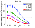
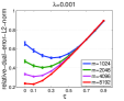
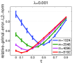
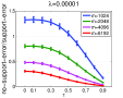
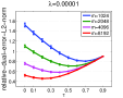
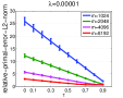
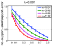
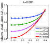
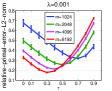
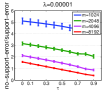
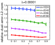
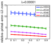
Figure 1: Recovery error for squared hinge loss. From left to right: $\frac{\|[\widetilde{\alpha}_{*}]_{\mathcal{S}^{c}}\|_{1}}{\|[\widetilde{\alpha}_{*}]_{\mathcal{S}}-[\alpha_{*}]_{\mathcal{S}}\|_{1}}$ vs $\tau$, $\frac{\|\widetilde{\alpha}_{*}-\alpha_{*}\|_{2}}{\|\alpha_{*}\|_{2}}$ vs $\tau$, and $\frac{\|\widetilde{\mathbf{w}}_{*}-\mathbf{w}_{*}\|_{2}}{\|\mathbf{w}_{*}\|_{2}}$ vs $\tau$.

Figure 2: Same curves as above but for non-smooth hinge loss.

An application to distributed learning. Although in some cases the solution learned in the reduced space can provide sufficiently good performance, it usually performs worse than the optimal solution that solves the original problem and sometimes the performance gap between them can not be ignored as seen in following experiments. To address this issue, we combine the benefits of distributed learning and the proposed randomized reduction methods for solving big data problems. When data is too large and sits on multiple machines, distributed learning can be employed to solve the optimization problem. In distributed learning, individual machines iteratively solve sub-problems associated with the subset of data on them and communicate some global variables (e.g., the primal solution $\mathbf{w}\in\mathbb{R}^{d}$) among them. When the dimensionality $d$ is very large, the total communication cost could be very high. To reduce the total communication cost, we propose to first solve the reduced data problem and then use the found solution as the initial solution to the distributed learning for the original data.

Below, we demonstrate the effectiveness of DSRR for the recently proposed distributed stochastic dual coordinate ascent (DisDCA) algorithm (Yang, 2013). The procedure is (1) reduce original high-dimensional data to very low dimensional space on individual machines; (2) use DisDCA to solve the reduced problem; (3) use the optimal dual solution to the reduce problem as an initial solution to DisDCA for solving the original problem. We record the running time for randomized reduction in step 1 and optimization of the reduced problem in step 2, and the optimization of the original problem in step 3. We compare the performance of four methods (i) the DSRR method that uses the model of the reduced problem solved by DisDCA to make predictions, (ii) the method that uses the recovered model in the original space, referred to as DSRR-Rec; (iii) the method that uses the dual solution to the reduced problem as an initial solution of DisDCA and runs it for the original problem with $k=1$ or $2$ communications (the number of updates before each communication is set to the number of examples in each machine), referred to as DSRR-DisDCA-$k$; and (iv) the distributed method that directly solves the original problem by DisDCA. For DisDCA to solve the original problem, we stop running when its performance on the testing data does not improve. Two data sets are used, namely RCV1-binary, KDD 2010 Cup data. For KDD 2010 Cup data, we use the one available on LibSVM data website. The statistics of the two data sets are summarized in Table 1. The results averaged over 5 trials are shown in Figure 3, which exhibit that the performance of DSRR-DisDCA-1/2 is remarkable in the sense that it achieves almost the same performance of directly training on the original data (DisDCA) and uses much less training time. In addition, DSRR-DisDCA performs much better than DSRR and has small computational overhead.

Table 1: Statistics of datasets

Name	#Training	#Testing	#Features	#Nodes
RCV1	677,399	20,242	47, 236	5
KDD	8,407,752	748,401	29,890,095	10

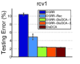
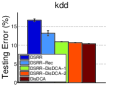
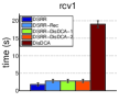
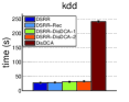
Figure 3: Top: Testing error for different methods. Bottom: Training time for different methods. The value of $\lambda=10^{-5}$ and the value of $\tau=0.9$. The high-dimensional features are reduced to $m=1024$-dimensional space using random hashing. The loss function is the squared hinge loss.

6 Conclusions

In this paper, we have proposed dual-sparse regularized randomized reduction methods for classification. We presented rigorous theoretical analysis of the proposed dual-sparse randomized reduction methods in terms of recovery error under a mild condition that the optimal dual variable is (nearly) sparse for both smooth and non-smooth loss functions, and for various randomized reduction approaches. The numerical experiments validate our theoretical analysis and also demonstrate that the proposed reduction and recovery framework can benefit distributed optimization by providing a good initial solution.

Appendix A Proof of Theorem 1

Let $\widehat{F}(\alpha)$ be defined as

$$\widehat{F}(\alpha)=\frac{1}{n}\sum_{i=1}^{n}\ell_{i}^{*}(\alpha_{i})+\frac{1}{2\lambda n^{2}}\alpha^{T}\widehat{X}^{\top}\widehat{X}\alpha+\frac{\tau}{n}\|\alpha\|_{1}$$

Since $\widetilde{\alpha}_{*}=\arg\min\widehat{F}(\alpha)$ therefore for any $g_{*}\in\partial\|\alpha_{*}\|_{1}$

$$0\geq \hat{F}(\widetilde{\alpha}_{*})-\hat{F}(\alpha_{*})$$

$$\geq (\widetilde{\alpha}_{*}-\alpha_{*})^{\top}\left(\frac{1}{n}\nabla\ell^{*}(\alpha_{*})+\frac{1}{\lambda n^{2}}\widehat{X}^{\top}\widehat{X}\alpha_{*}\right)$$

$$+\frac{\tau}{n}(\widetilde{\alpha}_{*}-\alpha_{*})^{\top}g_{*}+\frac{1}{2nL}\|\widetilde{\alpha}_{*}-\alpha_{*}\|_{2}^{2}$$

where we used the strong convexity of $\ell_{i}^{*}$ and its strong convexity modulus $1/L$. By the optimality condition of $\alpha_{*}$, we can have

$$0 \geq(\alpha_{*}-\widetilde{\alpha}_{*})^{\top}\left(\frac{1}{n}\nabla\ell^{*}(\alpha_{*})+\frac{1}{\lambda n^{2}}X^{\top}X\alpha_{*}\right)$$ (16)

Combining the above two inequalities we have

$$0\geq (\widetilde{\alpha}_{*}-\alpha_{*})^{\top}\frac{1}{n}\Delta+\frac{\tau}{n}(\widetilde{\alpha}_{*}-\alpha_{*})^{\top}g_{*}+\frac{1}{2nL}\|\widetilde{\alpha}_{*}-\alpha_{*}\|_{2}^{2}$$

Since the above inequality holds for any $g_{*}\in\partial\|\alpha_{*}\|_{1}$, if we choose $[g_{*}]_{i}=sign([\widetilde{\alpha}_{*}]_{i}),i\in\mathcal{S}^{c}$, then we have

$$(\widetilde{\alpha}_{*}-\alpha_{*})^{\top}g_{*}\geq-\|[\widetilde{\alpha}_{*}]_{\mathcal{S}}-[\alpha_{*}]_{\mathcal{S}}\|_{1}+\|[\widetilde{\alpha}_{*}]_{\mathcal{S}^{c}}\|_{1}$$

Combining the above inequalities leads to

$$(\tau+\|\Delta\|_{\infty})\|[\widetilde{\alpha}_{*}]_{\mathcal{S}}-[\alpha_{*}]_{\mathcal{S}}\|_{1}\geq (\tau-\|\Delta\|_{\infty})\|[\widetilde{\alpha}_{*}]_{\mathcal{S}^{c}}\|_{1}$$

$$+\frac{1}{2L}\|\widetilde{\alpha}_{*}-\alpha_{*}\|_{2}^{2}$$ (17)

Assuming $\tau\geq 2\|\Delta\|_{\infty}$, we have

$$\|\widetilde{\alpha}_{*}-\alpha_{*}\|_{2}^{2}\leq 3\tau L\|[\widetilde{\alpha}_{*}]_{\mathcal{S}}-[\alpha_{*}]_{\mathcal{S}}\|_{1}$$ (18)

$$\|[\widetilde{\alpha}_{*}]_{\mathcal{S}^{c}}\|_{1}\leq 3\|[\widetilde{\alpha}_{*}]_{\mathcal{S}}-[\alpha_{*}]_{\mathcal{S}}\|_{1}$$

Therefore,

$$\|[\widetilde{\alpha}_{*}-\alpha_{*}]_{\mathcal{S}}\|_{1}^{2}\leq s\|\widetilde{\alpha}_{*}-\alpha_{*}\|_{2}^{2} \leq 3\tau Ls\|[\widetilde{\alpha}_{*}]_{\mathcal{S}}-[\alpha_{*}]_{\mathcal{S}}\|_{1}$$

leading to the result

$$\|[\widetilde{\alpha}_{*}]_{\mathcal{S}}-[\alpha_{*}]_{\mathcal{S}}\|_{1}\leq 3\tau Ls.$$

Combing this inequality with inequalities in (18) we have

$$\|[\widetilde{\alpha}_{*}]_{\mathcal{S}^{c}}\|_{1}\leq 9\tau Ls,\quad\|\widetilde{\alpha}_{*}-\alpha_{*}\|_{2}\leq 3\tau L\sqrt{s}.$$

Appendix B Proof of Theorem 3

Following the same proof of Theorem 1, we first notice that inequality (A) holds for $L=\infty$, i.e.,

$$(\tau+\|\Delta\|_{\infty})\|[\widetilde{\alpha}_{*}]_{\mathcal{S}}-[\alpha_{*}]_{\mathcal{S}}\|_{1}\geq (\tau-\|\Delta\|_{\infty})\|[\widetilde{\alpha}_{*}]_{\mathcal{S}^{c}}\|_{1}$$

Therefore if $\tau\geq 2\|\Delta\|_{\infty}$, we have

$$\|[\widetilde{\alpha}_{*}]_{\mathcal{S}^{c}}\|_{1}\leq 3\|[\widetilde{\alpha}_{*}]_{\mathcal{S}}-[\alpha_{*}]_{\mathcal{S}}\|_{1}$$

As a result,

$$\frac{\|\widetilde{\alpha}_{*}-\alpha_{*}\|_{1}}{\|\widetilde{\alpha}_{*}-\alpha_{*}\|_{2}} \leq\frac{\|[\widetilde{\alpha}_{*}]_{\mathcal{S}}-[\alpha_{*}]_{\mathcal{S}}\|_{1}+\|[\widetilde{\alpha}_{*}]_{\mathcal{S}^{c}}\|_{1}}{\|\widetilde{\alpha}_{*}-\alpha_{*}\|_{2}}$$

$$\leq\frac{4\|[\widetilde{\alpha}_{*}]_{\mathcal{S}}-[\alpha_{*}]_{\mathcal{S}}\|_{1}}{\|\widetilde{\alpha}_{*}-\alpha_{*}\|_{2}}\leq 4\sqrt{s}$$

By the definition of $\mathcal{K}_{n,s}$, we have $\displaystyle\frac{\widetilde{\alpha}_{*}-\alpha_{*}}{\|\widetilde{\alpha}_{*}-\alpha_{*}\|_{2}}\in\mathcal{K}_{n,16s}$. To proceed the proof, there exists $\widetilde{g}_{*}\in\partial|\widetilde{\alpha}_{*}|_{1}$ such that

$$0\geq (\widetilde{\alpha}_{*}-\alpha_{*})^{\top}\left(\frac{1}{n}\nabla\ell^{*}(\widetilde{\alpha}_{*})+\frac{1}{\lambda n^{2}}\widehat{X}^{\top}\widehat{X}\widetilde{\alpha}_{*}\right)$$

$$+\frac{\tau}{n}(\widetilde{\alpha}_{*}-\alpha_{*})^{\top}\widetilde{g}_{*}$$

Adding the above inequality with  (16), we have

$$0 \geq(\alpha_{*}-\widetilde{\alpha}_{*})^{\top}\left(\frac{1}{n}\nabla\ell^{*}(\alpha_{*})-\frac{1}{n}\nabla\ell^{*}(\widetilde{\alpha}_{*})\right)$$

$$+(\alpha_{*}-\widetilde{\alpha}_{*})^{\top}\left(\frac{1}{\lambda n^{2}}X^{\top}X\alpha_{*}-\frac{1}{\lambda n^{2}}\widehat{X}^{\top}\widehat{X}\widetilde{\alpha}_{*}\right)$$

$$+\frac{\tau}{n}\left\|[\widetilde{\alpha}_{*}]_{\mathcal{S}^{c}}\right\|_{1}-\frac{\tau}{n}\left\|[\widetilde{\alpha}_{*}]_{\mathcal{S}}-[\alpha_{*}]_{\mathcal{S}}\right\|_{1}$$

By convexity of $\ell^{*}$ we have

$$(\alpha_{*}-\widetilde{\alpha}_{*})^{\top}\left[\frac{1}{n}\nabla\ell^{*}(\alpha_{*})-\frac{1}{n}\nabla\ell^{*}(\widetilde{\alpha}_{*})\right]\geq 0$$

Thus, we have

$$\tau \left\|[\widetilde{\alpha}_{*}]_{\mathcal{S}}-[\alpha_{*}]_{\mathcal{S}}\right\|_{1}\geq\tau\left\|[\widetilde{\alpha}_{*}]_{\mathcal{S}^{c}}\right\|_{1}$$

$$+(\alpha_{*}-\widetilde{\alpha}_{*})^{\top}\left(\frac{1}{\lambda n}X^{\top}X-\frac{1}{\lambda n}\widehat{X}^{\top}\widehat{X}\right)\alpha_{*}$$

$$-(\alpha_{*}-\widetilde{\alpha}_{*})^{\top}\left(\frac{1}{\lambda n}X^{\top}X-\frac{1}{\lambda n}\widehat{X}^{\top}\widehat{X}\right)(\alpha_{*}-\widetilde{\alpha}_{*})$$

$$+\frac{1}{\lambda n}(\alpha_{*}-\widetilde{\alpha}_{*})^{\top}X^{\top}X(\alpha_{*}-\widetilde{\alpha}_{*})$$

Since

$$(\alpha_{*}-\widetilde{\alpha}_{*})^{\top}\Delta\geq-\|\Delta\|_{\infty}\|\alpha_{*}-\widetilde{\alpha}_{*}\|_{1},$$

and $\tau\geq 2\|\Delta\|_{\infty}$ and by the definition of $\rho^{-}_{s},\sigma_{s}$, we have

$$\frac{3\tau}{2} \left\|[\widetilde{\alpha}_{*}-\alpha_{*}]_{\mathcal{S}}\right\|_{1}\geq\frac{\tau}{2}\left\|[\widetilde{\alpha}_{*}]_{\mathcal{S}^{c}}\right\|_{1}$$

$$+\frac{\rho^{-}_{16s}-\sigma_{16s}}{\lambda n}\|\widetilde{\alpha}_{*}-\alpha_{*}\|_{2}^{2}$$

Then the conclusion follows the same analysis as before.

Appendix C Proof of Theorem 4

Let $\hat{F}(\alpha)$ be defined as

$$\hat{F}(\alpha)=\frac{1}{n}\sum_{i=1}^{n}\ell_{i}^{*}(\alpha_{i})+\frac{1}{2\lambda n^{2}}\alpha^{T}\widehat{X}^{\top}\widehat{X}\alpha+\frac{\tau}{n}\|\alpha\|_{1}$$

and $F(\alpha)$ be defined as

$$F(\alpha)=\frac{1}{n}\sum_{i=1}^{n}\ell_{i}^{*}(\alpha_{i})+\frac{1}{2\lambda n^{2}}\alpha^{T}X^{\top}X\alpha$$

Since $\widetilde{\alpha}_{*}=\arg\min\hat{F}(\alpha)$ therefore for any $g_{*}\in\partial\|\alpha^{s}_{*}\|_{1}$

$$0\geq \hat{F}(\widetilde{\alpha}_{*})-\hat{F}(\alpha^{s}_{*})$$

$$\geq (\widetilde{\alpha}_{*}-\alpha^{s}_{*})^{\top}\left(\frac{1}{n}\nabla\ell^{*}(\alpha^{s}_{*})+\frac{1}{\lambda n^{2}}\widehat{X}^{\top}\widehat{X}\alpha^{s}_{*}\right)$$

$$+\frac{\tau}{n}(\widetilde{\alpha}_{*}-\alpha^{s}_{*})^{\top}g_{*}+\frac{1}{2nL}\|\widetilde{\alpha}_{*}-\alpha^{s}_{*}\|_{2}^{2}$$

where we used the strong convexity of $\ell_{i}^{*}$ and its strong convexity modulus $1/L$. Due to the sub-optimality of $\alpha^{s}_{*}$, we have

$$\frac{1}{n}\|\alpha^{s}_{*}-\widetilde{\alpha}_{*}\|_{1}\xi \geq(\widetilde{\alpha}_{*}-\alpha^{s}_{*})^{\top}\left[\frac{1}{n}\nabla\ell^{*}(\alpha^{s}_{*})+\frac{1}{\lambda n^{2}}X^{\top}X\alpha^{s}_{*}\right]$$

Combining the above two inequalities we have

$$\frac{1}{n}\|\alpha^{s}_{*}-\widetilde{\alpha}_{*}\|_{1}\xi\geq (\widetilde{\alpha}_{*}-\alpha^{s}_{*})^{\top}\left(\frac{1}{\lambda n^{2}}(\widehat{X}\widehat{X}^{\top}-XX^{\top})\alpha^{s}_{*}\right)$$

$$+\frac{\tau}{n}(\widetilde{\alpha}_{*}-\alpha^{s}_{*})^{\top}g_{*}+\frac{1}{2nL}\|\widetilde{\alpha}_{*}-\alpha^{s}_{*}\|_{2}^{2}$$

Since the above inequality holds for any $g_{*}\in\partial\|\alpha^{s}_{*}\|_{1}$, if we choose $[g_{*}]_{i}=sign([\widetilde{\alpha}_{*}]_{i}),i\in\mathcal{S}^{c}$, then we have

$$(\xi+\tau)\|[\widetilde{\alpha}_{*}]_{\mathcal{S}}-[\alpha_{*}]_{\mathcal{S}}\|_{1}\geq-\|\Delta\|_{\infty}\|\widetilde{\alpha}_{*}-\alpha^{s}_{*}\|_{1}$$ (19)

$$+(\tau-\xi)\|[\widetilde{\alpha}_{*}]_{\mathcal{S}^{c}}\|_{1}+\frac{1}{2L}\|\widetilde{\alpha}_{*}-\alpha^{s}_{*}\|_{2}^{2}$$ (20)

Thus

$$(\tau+\xi+\|\Delta\|_{\infty})\|[\widetilde{\alpha}_{*}]_{\mathcal{S}}-[\alpha_{*}]_{\mathcal{S}}\|_{1}$$

$$\geq(\tau-\xi-\|\Delta\|_{\infty})\|[\widetilde{\alpha}_{*}]_{\mathcal{S}^{c}}\|_{1}+\frac{1}{2L}\|\widetilde{\alpha}_{*}-\alpha^{s}_{*}\|_{2}^{2}$$

Assuming $\tau\geq 2(\|\Delta\|_{\infty}+\xi)$, we have

$$\|\widetilde{\alpha}_{*}-\alpha^{s}_{*}\|_{2}^{2}\leq 3\tau L\|[\widetilde{\alpha}_{*}]_{\mathcal{S}}-[\alpha_{*}]_{\mathcal{S}}\|_{1}$$ (21)

$$\|[\widetilde{\alpha}_{*}]_{\mathcal{S}^{c}}\|_{1}\leq 3\|[\widetilde{\alpha}_{*}]_{\mathcal{S}}-[\alpha_{*}]_{\mathcal{S}}\|_{1}$$

Therefore,

$$\frac{\|[\widetilde{\alpha}_{*}]_{\mathcal{S}}-[\alpha_{*}]_{\mathcal{S}}\|_{1}^{2}}{s}\leq\|\widetilde{\alpha}_{*}-\alpha^{s}_{*}\|_{2}^{2} \leq 3\tau L\|[\widetilde{\alpha}_{*}]_{\mathcal{S}}-[\alpha_{*}]_{\mathcal{S}}\|_{1}$$

leading to the result

$$\|[\widetilde{\alpha}_{*}]_{\mathcal{S}}-[\alpha_{*}]_{\mathcal{S}}\|_{1}\leq 3\tau Ls$$

Combing above inequality with inequalities in (18) we have

$$\|[\widetilde{\alpha}_{*}]_{\mathcal{S}^{c}}\|_{1}\leq 9\tau Ls,\quad\|\widetilde{\alpha}_{*}-\alpha^{s}_{*}\|_{2}\leq 3\tau L\sqrt{s}.$$

Appendix D Proof of Theorem 7

Recall the definition of $\mathcal{S}_{n,s}$:

$$\mathcal{S}_{n,s}=\{\alpha\in\mathbb{R}^{n}:\|\alpha\|_{2}\leq 1,\|\alpha\|_{0}\leq s\}$$

Due to $conv(\mathcal{S}_{n,s})\subset\mathcal{K}_{n,s}\subset 2conv(\mathcal{S}_{n,s})$, for any $\alpha\in\mathcal{K}_{n,s}$, we can write it as $\alpha=2\sum_{i}\lambda_{i}\beta_{i}$ where $\beta_{i}\in\mathcal{S}_{n,s}$, $\sum_{i}\lambda_{i}=1$ and $\lambda_{i}\geq 0$, then we have

$$|(X\alpha)^{\top}(I-A^{\top}A)(X\alpha)|$$

$$\leq 4\left|\left(X\sum_{i}\lambda_{i}\beta_{i}\right)^{\top}(I-A^{\top}A)\left(X\sum_{i}\lambda_{i}\beta_{i}\right)\right|$$

$$\leq 4\sum_{ij}\lambda_{i}\lambda_{j}|(X\beta_{i})^{\top}(I-A^{\top}A)(X\beta_{j})|$$

$$\leq 4\max_{\alpha_{1},\alpha_{2}\in\mathcal{S}_{n,s}}|(X\alpha_{1})^{\top}(I-A^{\top}A)(X\alpha_{2})|\sum_{ij}\lambda_{i}\lambda_{j}$$

$$=4\max_{\alpha_{1},\alpha_{2}\in\mathcal{S}_{n,s}}|(X\alpha_{1})^{\top}(I-A^{\top}A)(X\alpha_{2})$$

Therefore

$$\max_{\alpha\in\mathcal{K}_{n,s}}|(X\alpha)^{\top}(I-A^{\top}A)(X\alpha)|$$

$$\leq 4\max_{\alpha_{1},\alpha_{2}\in\mathcal{S}_{n,s}}|(X\alpha_{1})^{\top}(I-A^{\top}A)(X\alpha_{2})$$

Let $\mathbf{u}_{1}=X\alpha_{1}$ and $\mathbf{u}_{2}=X\alpha_{2}$. Following the Proof of Theorem 5, for any fixed $\alpha_{1},\alpha_{2}\in\mathcal{S}_{n,s}$, with a probability $1-2\delta$ we have

$$\frac{1}{n}|(X\alpha_{1})^{\top}(I-A^{\top}A)(X\alpha_{2})|$$

$$\leq\frac{1}{n}\|X\alpha_{1}\|_{2}\|X\alpha_{2}\|_{2}\epsilon_{A,\delta}\leq\rho_{s}^{+}\epsilon_{A,\delta}\leq O\left(\rho^{+}_{s}\sqrt{\frac{\log(1/\delta)}{m}}\right)$$

where we use

$$\max_{\alpha\in\mathcal{S}_{n,s}}\frac{\|X\alpha\|_{2}}{\sqrt{n}}\leq\max_{\alpha\in\mathcal{K}_{n,s}}\frac{\|X\alpha\|_{2}}{\sqrt{n}}=\sqrt{\rho^{+}_{s}}$$

In order to extend the inequity to all $\alpha_{1},\alpha_{2}\in\mathcal{S}_{n,s}$. We consider the $\epsilon$ proper-net of $\mathcal{S}_{n,s}$ (Plan & Vershynin, 2011) denoted by $\mathcal{S}_{n,s}(\epsilon)$. Lemma 3.3 in (Plan & Vershynin, 2011) shows that the entropy of $\mathcal{S}_{d,s}$, i.e., the cardinality of $\mathcal{S}_{n,s}(\epsilon)$ denoted $N(\mathcal{S}_{n,s},\epsilon)$ is bounded by

$$\log N(\mathcal{S}_{n,s},\epsilon)\leq s\log\left(\frac{9n}{\epsilon s}\right)$$

Then by using the union bound, we have with a probability $1-2\delta$, we have

$$\max_{\alpha_{1}\in\mathcal{S}_{n,s}(\epsilon)\atop\alpha_{2}\in\mathcal{S}_{n,s}(\epsilon)}\frac{1}{n}|(X\alpha_{1})^{\top}(I-A^{\top}A)(X\alpha_{2})|$$

$$\leq O\left(\rho^{+}_{s}\sqrt{\frac{\log(N^{2}(\mathcal{S}_{n,s},\epsilon)/\delta)}{m}}\right)$$

$$\leq O\left(\rho^{+}_{s}\sqrt{\frac{\log(1/\delta)+2s\log(9n/\epsilon s)}{m}}\right)$$ (22)

To proceed the proof, we need the following lemma.

Lemma 5.

Let

$$\mathcal{E}_{s}(\alpha_{2})=\max_{\alpha_{1}\in\mathcal{S}_{n,s}}|\alpha_{1}^{\top}U\alpha_{2}|$$

$$\mathcal{E}_{s}(\alpha_{2},\epsilon)=\max_{\alpha_{1}\in\mathcal{S}_{n,s}(\epsilon)}|\alpha_{1}^{\top}U\alpha_{2}|$$

For $\epsilon\in(0,1/\sqrt{2})$, we have

$$\mathcal{E}_{s}(\alpha_{2})\leq\left(\frac{1}{1-\sqrt{2}\epsilon}\right)\mathcal{E}_{s}(\alpha_{2},\epsilon)$$

Proof.

Let $U=\frac{1}{n}X^{\top}(I-A^{\top}A)X$. Following Lemma 9.2 of (Koltchinskii, 2011), for any $\alpha,\alpha^{\prime}\in\mathcal{S}_{n,s}$, we can always find two vectors $\beta$, $\beta^{\prime}$ such that

$$\alpha-\alpha^{\prime}=\beta-\beta^{\prime},\ \|\beta\|_{0}\leq s,\ \|\beta^{\prime}\|_{0}\leq s,\ \beta^{\top}\beta^{\prime}=0.$$

Let

$$\mathcal{E}_{s}(\alpha_{2})=\max_{\alpha_{1}\in\mathcal{S}_{n,s}}|\alpha_{1}^{\top}U\alpha_{2}|$$

$$\mathcal{E}_{s}(\alpha_{2},\epsilon)=\max_{\alpha_{1}\in\mathcal{S}_{n,s}(\epsilon)}|\alpha_{1}^{\top}U\alpha_{2}|$$

Thus

$$\begin{split}&|\langle\alpha-\alpha^{\prime},U\alpha_{2}\rangle|\leq|\langle\beta,U\alpha_{2}\rangle|+|\langle-\beta^{\prime},U\alpha_{2}\rangle|\\ =&\|\beta\|_{2}\left|\left\langle\frac{\beta}{\|\beta\|_{2}},U\alpha_{2}\right\rangle\right|+\|\beta^{\prime}\|_{2}\left|\left\langle\frac{-\beta^{\prime}}{\|\beta^{\prime}\|_{2}},U\alpha_{2}\right\rangle\right|\\ \leq&(\|\beta\|_{2}+\|\beta^{\prime}\|_{2})\mathcal{E}_{s}(\alpha_{2})\leq\mathcal{E}_{s}(\alpha_{2})\sqrt{2}\sqrt{\|\beta\|_{2}^{2}+\|\beta^{\prime}\|_{2}^{2}}\\ =&\mathcal{E}_{s}(\alpha_{2})\sqrt{2}\|\beta-\beta^{\prime}\|_{2}=\mathcal{E}_{s}(\alpha_{2})\sqrt{2}\|\beta-\beta^{\prime}\|_{2}\\ =&\mathcal{E}_{s}(\alpha_{2})\sqrt{2}\|\alpha-\alpha^{\prime}\|_{2}.\end{split}$$

Then, we have

$$\begin{split}&\mathcal{E}_{s}(\alpha_{2})=\max\limits_{\alpha\in\mathcal{S}_{n,s}}|\alpha^{\top}U\alpha_{2}|\\ \leq&\max\limits_{\alpha\in\mathcal{S}_{n,s}(\epsilon)}|\alpha^{\top}U\alpha_{2}|+\sup_{\alpha\in\mathcal{S}_{n,s}\atop\alpha^{\prime}\in\mathcal{S}_{n,s}(\epsilon),\|\alpha-\alpha^{\prime}\|_{2}\leq\epsilon}\langle\alpha-\alpha^{\prime},U\alpha_{2}\rangle\\ \leq&\mathcal{E}_{s}(\alpha_{2},\epsilon)+\sqrt{2}\epsilon\mathcal{E}_{s}(\alpha_{2})\end{split}$$

which implies

$$\mathcal{E}_{s}(\alpha_{2})\leq\frac{\mathcal{E}_{s}(\alpha_{2},\epsilon)}{1-\sqrt{2}\epsilon}.$$

∎

Lemma 6.

Let

$$\mathcal{E}_{s}(\epsilon)=\max_{\alpha_{2}\in\mathcal{S}_{n,s}}\mathcal{E}_{s}(\alpha_{2},\epsilon)=\max_{\alpha_{1}\in\mathcal{S}_{n,s}\atop\alpha_{2}\in\mathcal{S}_{n,s}(\epsilon)}|\alpha_{1}^{\top}U\alpha_{2}|$$

$$\mathcal{E}_{s}(\epsilon,\epsilon)=\max_{\alpha_{2}\in\mathcal{S}_{n,s}(\epsilon)}\mathcal{E}_{s}(\alpha_{2},\epsilon)=\max_{\alpha_{1},\alpha_{2}\in\mathcal{S}_{n,s}(\epsilon)}|\alpha_{1}^{\top}U\alpha_{2}|$$

For $\epsilon\in(0,1/\sqrt{2})$, we have

$$\mathcal{E}_{s}(\epsilon)\leq\left(\frac{1}{1-\sqrt{2}\epsilon}\right)\mathcal{E}_{s}(\epsilon,\epsilon)$$

The proof the above lemma follows the same analysis as that of Lemma 1. By combining Lemma 1 and Lemma 2, we have

$$\sigma_{s}=\max_{\alpha_{2}\in\mathcal{S}_{n,s}}\mathcal{E}_{s}(\alpha_{2})\leq\frac{\max_{\alpha_{2}\in\mathcal{S}_{n,s}}\mathcal{E}_{s}(\alpha_{2},\epsilon)}{1-\sqrt{2}\epsilon}$$

$$=\frac{1}{1-\sqrt{2}\epsilon}\mathcal{E}_{s}(\epsilon)\leq\left(\frac{1}{1-\sqrt{2}\epsilon}\right)^{2}\mathcal{E}_{s}(\epsilon,\epsilon)$$

$$=\left(\frac{1}{1-\sqrt{2}\epsilon}\right)^{2}\max_{\alpha_{1},\alpha_{2}\in\mathcal{S}_{n,s}(\epsilon)}|\alpha_{1}^{\top}U\alpha_{2}|$$

By combing the above inequality with inequality (D), we have

$$\sigma_{s}\leq\left(\frac{1}{1-\sqrt{2}\epsilon}\right)^{2}O\left(\rho^{+}_{s}\sqrt{\frac{\log(1/\delta)+2s\log(9n/\epsilon s)}{m}}\right)$$

References

• Achlioptas (2003) Achlioptas, Dimitris. Database-friendly random projections: Johnson-lindenstrauss with binary coins. Journal of Computer and System Sciences., 66:671–687, 2003.
• Agarwal et al. (2011) Agarwal, Alekh, Chapelle, Olivier, Dud k, Miroslav, and Langford, John. A reliable effective terascale linear learning system. CoRR, 2011.
• Ailon & Chazelle (2009) Ailon, Nir and Chazelle, Bernard. The fast johnson–lindenstrauss transform and approximate nearest neighbors. SIAM J. Comput., 39(1):302–322, 2009.
• Balcan et al. (2006) Balcan, Maria-Florina, Blum, Avrim, and Vempala, Santosh. Kernels as features: On kernels, margins, and low-dimensional mappings. Machine Learning, 65:79–94, 2006.
• Bartz et al. (2011) Bartz, Daniel, Hatrick, Kerr, Hesse, Christian W., Müller, Klaus-Robert, and Lemm, Steven. Directional variance adjustment: improving covariance estimates for high-dimensional portfolio optimization. arXiv:1109.3069, 2011.
• Ben-Hur et al. (2008) Ben-Hur, Asa, Ong, Cheng Soon, Sonnenburg, Sören, Schölkopf, Bernhard, and Rätsch, Gunnar. Support vector machines and kernels for computational biology. PLoS Comput Biology, 4:e1000173, 2008.
• Bickel et al. (2009) Bickel, Peter J., Ritov, Ya’acov, and Tsybakov, Alexandre B. Simultaneous analysis of lasso and dantzig selector. ANNALS OF STATISTICS, 37(4), 2009.
• Blum (2005) Blum, Avrim. Random projection, margins, kernels, and feature-selection. In Proceedings of the 2005 International Conference on Subspace, Latent Structure and Feature Selection, volume 3940, pp.  52–68. Springer, 2005.
• Boyd & Vandenberghe (2004) Boyd, Stephen and Vandenberghe, Lieven. Convex Optimization. Cambridge University Press, 2004.
• Brank et al. (2002) Brank, Janez, Grobelnik, Marko, Milić-Frayling, Natasa, and Mladenić, D. Feature selection using support vector machines. In Proceedings of the International Conference on Data Mining Methods and Databases for Engineering, Finance, and Other Fields, pp. 84–89, 2002.
• Dasgupta et al. (2010) Dasgupta, Anirban, Kumar, Ravi, and Sarlós, Tamás. A sparse johnson–lindenstrauss transform. In Proceedings of the 42nd ACM symposium on Theory of computing, STOC ’10, pp.  341–350, 2010.
• Drineas et al. (2006) Drineas, Petros, Mahoney, Michael W., and Muthukrishnan, S. Sampling algorithms for l2 regression and applications. In ACM-SIAM Symposium on Discrete Algorithms (SODA), pp. 1127–1136, 2006.
• Drineas et al. (2008) Drineas, Petros, Mahoney, Michael W., and Muthukrishnan, S. Relative-error cur matrix decompositions. SIAM Journal Matrix Analysis Applications, 30:844–881, 2008.
• Drineas et al. (2011) Drineas, Petros, Mahoney, Michael W., Muthukrishnan, S., and Sarlós, Tamàs. Faster least squares approximation. Numerische Mathematik, 117(2):219–249, February 2011.
• Eldar & Kutyniok (2012) Eldar, Yonina C. and Kutyniok, Gitta. Compressed Sensing: Theory and Applications. Compressed Sensing: Theory and Applications. Cambridge University Press, 2012. ISBN 9781107005587.
• Goldberger et al. (2005) Goldberger, Jacob, Roweis, Sam, Hinton, Geoffrey, and Salakhutdinov, Ruslan. Neighbourhood components analysis. In Advances in Neural Information Processing Systems (NIPS), pp.  513–520, 2005.
• Guyon et al. (2002) Guyon, Isabelle, Weston, Jason, Barnhill, Stephen, and Vapnik, Vladimir. Gene selection for cancer classification using support vector machines. Machine Learning (ML), 46:389–422, 2002.
• Jaggi et al. (2014) Jaggi, Martin, Smith, Virginia, Takác, Martin, Terhorst, Jonathan, Krishnan, Sanjay, Hofmann, Thomas, and Jordan, Michael I. Communication-efficient distributed dual coordinate ascent. In Advances in Neural Information Processing Systems (NIPS), pp.  3068–3076, 2014.
• Jostins & Barrett (2011) Jostins, Luke and Barrett, Jeffrey C. Genetic risk prediction in complex disease. Human Molecular Genetics, 20(R2):R182–R188, 2011.
• Kane & Nelson (2014) Kane, Daniel M. and Nelson, Jelani. Sparser johnson-lindenstrauss transforms. Journal of the ACM, 61:4:1–4:23, 2014.
• Kang & Cho (2011) Kang, J., Kugathasan S. Georges M. Zhao H. and Cho, J.H. Improved risk prediction for crohn’s disease with a multi-locus approach. Human Molecular Genetics, 20:2435–2442, 2011.
• Koltchinskii (2011) Koltchinskii, V. Oracle Inequalities in Empirical Risk Minimization and Sparse Recovery Problems: École D’Été de Probabilités de Saint-Flour XXXVIII-2008. Ecole d’été de probabilités de Saint-Flour. Springer, 2011. ISBN 9783642221460.
• Lewis et al. (2004) Lewis, David D., Yang, Yiming, Rose, Tony G., and Li, Fan. Rcv1: A new benchmark collection for text categorization research. Journal of Machine Learning Research (JMLR), 5:361–397, 2004.
• Li et al. (2014) Li, Mu, Andersen, David G, Smola, Alex J, and Yu, Kai. Communication efficient distributed machine learning with the parameter server. In Advances in Neural Information Processing Systems (NIPS), pp.  19–27. 2014.
• Ma et al. (2014) Ma, Ping, Mahoney, Michael W., and Yu, Bin. A statistical perspective on algorithmic leveraging. In Proceedings of the 31th International Conference on Machine Learning (ICML), pp.  91–99, 2014.
• Mahoney (2011) Mahoney, Michael W. Randomized algorithms for matrices and data. Foundations and Trends in Machine Learning, 3(2):123–224, 2011.
• Mahoney & Drineas (2009) Mahoney, Michael W. and Drineas, Petros. Cur matrix decompositions for improved data analysis. Proceedings of the National Academy of Sciences, 106(3):697–702, 2009.
• Mitchell et al. (2004) Mitchell, Tom M., Hutchinson, Rebecca, Niculescu, Radu S., Pereira, Francisco, Wang, Xuerui, Just, Marcel, and Newman, Sharlene. Learning to decode cognitive states from brain images. Machine Learning, 57(1-2):145–175, 2004.
• (29) Nelson, Jelani. Johnson-lindenstrauss notes. Technical report, MIT.
• Paul et al. (2013) Paul, Saurabh, Boutsidis, Christos, Magdon-Ismail, Malik, and Drineas, Petros. Random projections for support vector machines. In Proceedings of the International Conference on Artificial Intelligence and Statistics (AISTATS), pp.  498–506, 2013.
• Plan & Vershynin (2011) Plan, Yaniv and Vershynin, Roman. One-bit compressed sensing by linear programming. CoRR, abs/1109.4299, 2011.
• Rätsch et al. (2005) Rätsch, G., Sonnenburg, S., and Schölkopf, B. RASE: recognition of alternatively spliced exons in c.elegans. Bioinformatics, 21:i369–i377, 2005.
• R tsch et al. (2005) R tsch, Gunnar, Sonnenburg, S ren, and Sch lkopf, Bernhard. Rase: recognition of alternatively spliced exons in c.elegans. In Proceedings of the International Conference on Intelligent Systems for Molecular Biology (ISMB) (Supplement of Bioinformatics), pp. 369–377, 2005.
• Sánchez et al. (2013) Sánchez, Jorge, Perronnin, Florent, Mensink, Thomas, and Verbeek, Jakob J. Image classification with the fisher vector: Theory and practice. International Journal of Computer Vision, 105(3):222–245, 2013.
• Shi et al. (2009a) Shi, Qinfeng, Petterson, James, Dror, Gideon, Langford, John, Smola, Alex, and Vishwanathan, S.V.N. Hash kernels for structured data. Journal of Machine Learning Research (JMLR), 10:2615–2637, 2009a.
• Shi et al. (2009b) Shi, Qinfeng, Petterson, James, Dror, Gideon, Langford, John, Smola, Alexander J., Strehl, Alexander L., and Vishwanathan, Vishy. Hash kernels. In Proceedings of the International Conference on Artificial Intelligence and Statistics (AISTATS), pp.  496–503, 2009b.
• Shi et al. (2012) Shi, Qinfeng, Shen, Chunhua, Hill, Rhys, and van den Hengel, Anton. Is margin preserved after random projection? In Proceedings of the International Conference on Machine Learning (ICML), 2012.
• Simianer et al. (2012) Simianer, Patrick, Riezler, Stefan, and Dyer, Chris. Joint feature selection in distributed stochastic learning for large-scale discriminative training in smt. In Proceedings of Annual Meeting of the Association for Computational Linguistics (ACL), pp.  11–21, 2012.
• Sonnenburg & Franc (2010) Sonnenburg, S ren and Franc, Vojtech. Coffin: A computational framework for linear svms. In Proceedings of the International Conference on Machine Learning (ICML), pp.  999–1006, 2010.
• Sonnenburg et al. (2007) Sonnenburg, S ren, Schweikert, Gabriele, Philips, Petra, Behr, Jonas, and R tsch, Gunnar. Accurate splice site prediction using support vector machines. BMC Bioinformatics, 8, 2007.
• Tropp (2011) Tropp, Joel A. Improved analysis of the subsampled randomized hadamard transform. Advances in Adaptive Data Analysis, 3(1-2):115–126, 2011.
• Weinberger et al. (2009) Weinberger, Kilian Q., Dasgupta, Anirban, Langford, John, Smola, Alexander J., and Attenberg, Josh. Feature hashing for large scale multitask learning. In Proceedings of the International Conference on Machine Learning (ICML), pp.  1113–1120, 2009.
• Xiao & Zhang (2013) Xiao, Lin and Zhang, Tong. A proximal-gradient homotopy method for the sparse least-squares problem. SIAM Journal on Optimization, 23(2):1062–1091, 2013.
• Yang (2013) Yang, Tianbao. Trading computation for communication: Distributed stochastic dual coordinate ascent. In Advances in Neural Information Processing Systems (NIPS), pp.  629–637, 2013.
• Zhang et al. (2013) Zhang, Lijun, Mahdavi, Mehrdad, Jin, Rong, Yang, Tianbao, and Zhu, Shenghuo. Recovering the optimal solution by dual random projection. In COLT, pp.  135–157, 2013.
• Zhang et al. (2014) Zhang, Lijun, Mahdavi, Mehrdad, Jin, Rong, Yang, Tianbao, and Zhu, Shenghuo. Random projections for classification: A recovery approach. IEEE Transactions on Information Theory (IEEE TIT), 60(11):7300–7316, 2014.