Efficient discontinuous Galerkin finite element methods via Bernstein polynomials

Abstract

We consider the discontinuous Galerkin method for hyperbolic conservation laws, with some particular attention to the linear acoustic equation, using Bernstein polynomials as local bases. Adapting existing techniques leads to optimal-complexity computation of the element and boundary flux terms. The element mass matrix, however, requires special care. In particular, we give an explicit formula for its eigenvalues and exact characterization of the eigenspaces in terms of the Bernstein representation of orthogonal polynomials. We also show a fast algorithm for solving linear systems involving the element mass matrix to preserve the overall complexity of the DG method. Finally, we present numerical results investigating the accuracy of the mass inversion algorithms and the scaling of total run-time for the function evaluation needed in DG time-stepping.

1 Introduction

Bernstein polynomials, which are “geometrically decomposed” in the sense of (arnold2009geometric, ) and rotationally symmetric, provide a flexible and general-purpose set of simplicial finite element shape functions. Morever, recent research has demonstrated distinct algorithmic advantages over other simplicial shape functions, as many essential elementwise finite element computations can be performed on with optimal complexity using Bernstein polynomials In (kirby2011fast, ), we showed how, with constant coefficients, elementwise mass and stiffness matrices could each be applied to vectors in $\mathcal{O}(n^{d+1})$ operations, where $n$ is the degree of the local basis and $d$ is the spatial dimension. Similar blockwise linear algebraic structure enabled quadrature-based algorithms in (kirby2012fast, ). Around the same time, Ainsworth et al (ainsworth2011bernstein, ) showed that the Duffy transform (duffy1982quadrature, ) reveals a tensorial structure in the Bernstein basis itself, leading to sum-factored algorithms for polynomial evaluation and moment computation. Moreover, they provide an algorithm that assembles element matrices with $\mathcal{O}(1)$ work per entry that utilizes their fast moment algorithm together with a very special property of the Bernstein polynomials. Work in (kirbyssec, ; brown_sc_2012_20, ) extends these techniques to $H(\mathrm{div})$ and $H(\mathrm{curl})$.

In this paper, we consider Bernstein polynomial techniques in a different context – discontinuous Galerkin methods for hyperbolic conservation laws

$$q_{t}+\nabla\cdot F(q)=0,$$ (1)

posed on a domain $\Omega\times[0,T)\subset\mathbb{R}^{d}\times\mathbb{R}$, together with suitable initial and boundary conditions. As a particular example, we consider the linear acoustic model

$$\begin{split}p_{t}+\nabla\cdot u&=0,\\ u_{t}+\nabla p&=0,\end{split}$$ (2)

Here, $q=[u,p]^{T}$ where the pressure variable $p$ is a scalar-valued function on $\Omega\times[0,T]$ and the velocity $u$ maps the same space-time domain into $\mathbb{R}^{d}$.

Discontinuous Galerkin (DG) methods for such problems place finite volume methods in a variational framework and extend them to higher orders of polynomial approximation cockburn1991runge , but fully realizing the potential efficiencies of high-order methods requires careful consideration of algorithmic issues. Simplicial orthogonal polynomials dubiner1991spectral ; KarShe05 provide one existing mechanism for achieving low operation counts. Their orthogonality gives diagonal local mass matrices. Optimality then requires special quadrature that reflects the tensorial nature of the basis under the Duffy transform or collapsed-coordinate mapping from the $d$-simplex to the $d$-cube and also includes appropriate points to incorporate contributions from both volume and boundary flux terms. Hesthaven and Warburton (hesthaven2002nodal, ; hesthaven2007nodal, ) propose an alternate approach, using dense linear algebra in conjunction with Lagrange polynomials. While of greater algorithmic complexity, highly-tuned matrix multiplication can make this approach competitive or even superior at practical polynomial orders. Additional extensions of this idea include the so-called “strong DG” forms and also a pre-elimination of the elementwise mass matrix giving rise to a simple ODE system. With care, this approach can give very high performance on both CPU and GPU systems (klockner2009nodal, ).

In this paper, we will show how each term in the DG formulation with Bernstein polynomials as the local basis can be handled with optimal complexity For the element and boundary flux terms, this requires only an adaptation of existing techniques, but inverting the element mass matrix turns out to be a challenge lest it dominate the complexity of the entire process. We rely on the recursive block structure described in (kirby2011fast, ) to give an $\mathcal{O}(n^{d+1})$ algorithm for solving linear systems with the constant-coefficient mass matrix. We may view our approach as sharing certain important features of both collapsed-coordinate and Lagrange bases. Like collapsed-coordinate methods, we seek to use specialized structure to optimize algorithmic complexity. Like Lagrange polynomials, we seek to do this using a relatively discretization-neutral basis.

2 Discontinuous Galerkin methods

We let $\mathcal{T}_{h}$ be a triangulation of $\Omega$ in the sense of  (BreSco, ) into affine simplices. For curved-sided elements, we could adapt the techniques of warburton2013low to incorporate the Jacobian into our local basis functions to recover the reference mass matrix on each cell at the expense of having variable coefficients in other operators, but this does not affect the overall order of complexity. We let $\mathcal{E}_{h}$ denote the set of all edges in the triangulation.

For $T\in\mathcal{T}_{h}$, let $P_{n}(T)$ be the space of polynomials of degree no greater than $n$ on $T$. This is a vector space of dimension $P^{d}_{n}\equiv\binom{n+d}{n}$. We define the global finite element space

$$V_{h}=\left\{f:\Omega\rightarrow\mathbb{R}:f|_{T}\in P_{n}(T),\ T\in\mathcal{T}_{h}\right\},$$ (3)

with no continuity enforced between cells. Let $\left(\cdot,\cdot\right)_{T}$ denote the standard $L^{2}$ inner product over $T\in\mathcal{T}_{h}$ and $\langle\cdot,\cdot\rangle_{\gamma}$ the $L_{2}$ inner product over an edge $\gamma\in\mathcal{E}_{h}$.

After multiplying (1) by a test function and integating by parts elementwise, a DG method seeks $u_{h}$ in $V_{h}$ such that

$$\sum_{T\in\mathcal{T}_{h}}\left[\left(u_{h,t},v_{h}\right)_{T}-\left(F(u_{h}),\nabla v_{h}\right)_{T}\right]+\sum_{\gamma\in\mathcal{E}_{h}}\langle\hat{F}\cdot n,v_{h}\rangle$$ (4)

for all $v_{h}\in V_{h}$.

Fully specifying the DG method requires defining a numerical flux function $\hat{F}$ on each $\gamma$. On internal edges, it takes values from either side of the edge and produces a suitable approximation to the flux $F$. Many Riemann solvers from the finite volume literature have been adapted for DG methods cockburn1991runge ; dumbser2008unified ; toro1999riemann . The particular choice of numerical flux does not matter for our purposes. On external edges, we choose $\hat{F}$ to appropriately enforce boundary conditions.

This discretization gives rise to a system of ordinary differential equations

$$\mathrm{M}\mathrm{u}_{t}+\mathrm{F}(\mathrm{u})=0,$$ (5)

where $\mathrm{M}$ is the block-diagonal mass matrix and $\mathrm{F}(\mathrm{u})$ includes the cell and boundary flux terms. Because of the hyperbolic nature of the system, explicit methods are frequently preferred. A forward Euler method, for example, gives

$$\mathrm{u}^{n+1}=\mathrm{u}^{n}-\Delta t\mathrm{M}^{-1}\mathrm{F}(\mathrm{u^{n}})\equiv\mathrm{u}^{n}-\Delta tL(\mathrm{u}^{n}),$$ (6)

which requires the application of $\mathrm{M}$ at each time step. The SSP methods gottlieb2001strong ; shu1988total give stable higher-order in time methods. For example, the well-known third order scheme is

$$\begin{split}\mathrm{u}^{n,1}&=\mathrm{u}^{n}+\Delta tL(\mathrm{u}^{n}),\\ \mathrm{u}^{n,2}&=\frac{3}{4}\mathrm{u}^{n}+\frac{1}{4}\mathrm{u}^{n,1}+\frac{1}{4}\Delta tL(\mathrm{u}^{n,1}),\\ \mathrm{u}^{n+1}&=\frac{1}{3}\mathrm{u}^{n}+\frac{2}{3}\mathrm{u}^{n,2}+\frac{2}{3}\Delta tL(\mathrm{u}^{n,2}).\end{split}$$ (7)

Since the Bernstein polynomials give a dense element mass matrix, applying $\mathrm{M}^{-1}$ efficiently will require some care. It turns out that $\mathrm{M}$ possesses many fascinating properties that we shall survey in Section 4. Among these, we will give an $\mathcal{O}(n^{d+1})$ algorithm for applying the elementwise inverse.

DG methods yield reasonable solutions to acoustic or Maxwell’s equations without slope limiters, although most nonlinear problems will require them to suppress oscillations. Even linear transport can require limiting when a discrete maximum principle is required. Limiting high-order polynomials on simplicial domains remains quite a challenge. It may be possible to utilize properties of the Bernstein polynomials to design new limiters or conveniently implement existing ones. For example, the convex hull property (i.e. that polynomials in the Bernstein basis lie in the convex hull of their control points) gives sufficient conditions for enforcing extremal bounds. We will not offer further contributions in this direction, but refer the reader to other works on higher order limiting such as (hoteit2004new, ; zhu2008runge, ; zhu2013runge, ).

3 Bernstein-basis finite element algorithms

3.1 Notation for Bernstein polynomials

We formulate Bernstein polynomials on the $d$-simplex using barycentric coordinates and multiindex notation. For a nondegenerate simplex $T\subset\mathbb{R}^{d}$ with vertices $\{x_{i}\}_{i=0}^{d}$, let $\{b_{i}\}_{i=0}^{d}$ denote the barycentric coordinates. Each $b_{i}$ affinely maps $\mathbb{R}^{d}$ into $\mathbb{R}$ with $b_{i}(x_{j})=\delta_{ij}$ for $0\leq i,j\leq d$. It follows that $b_{i}(x)\geq 0$ for all $x\in T$.

We will use common multiindex notation, denoting multiindices with Greek letters, although we will begin the indexing with 0 rather than 1. So, $\alpha=(\alpha_{0},\alpha_{1},\dots,\alpha_{d})$ is a tuple of $d+1$ nonnegative integers. We define the order of a multiindex $\alpha$ by $\left|\alpha\right|\equiv\sum_{i=0}^{d}\alpha_{i}$. We say that $\alpha\geq\beta$ provided that the inequality $\alpha_{i}\geq\beta_{i}$ holds componentwise for $0\leq i\leq d$. Factorials and binomial coefficients over multiindices have implied multiplication. That is,

$$\alpha!\equiv\prod_{i=0}^{d}\alpha_{i}!$$

and, provided that $\alpha\geq\beta$,

$$\binom{\alpha}{\beta}=\prod_{i=0}^{d}\binom{\alpha_{i}}{\beta_{i}}.$$

Without ambiguity of notation, we also define a binomial coefficient with a whole number for the upper argument and and multiindex as lower by

$$\binom{n}{\alpha}=\frac{n!}{\alpha!}=\frac{n!}{\prod_{i=0}^{n}\alpha_{i}!}.$$

We also define $e_{i}$ to be the multiindex consisting of zeros in all but the $i^{\mathrm{th}}$ entry, where it is one.

Let $\mathbf{b}\equiv\left(b_{0},b_{2},\dots,b_{d}\right)$ be a tuple of barycentric coordinates on a simplex. For multiindex $\alpha$, we define a barycentric monomial by

$$\mathbf{b}^{\alpha}=\prod_{i=0}^{d}b_{i}^{\alpha}.$$

We obtain the Bernstein polynomials by scaling these by certain binomial coefficients

$$B^{n}_{\alpha}=\frac{n!}{\alpha!}\mathbf{b}^{\alpha}.$$ (8)

For all spatial dimensions and degrees $n$, the Bernstein polynomials of degree $n$

$$\left\{B^{n}_{\alpha}\right\}_{\left|\alpha\right|=n},$$

form a nonnegative partition of unity and a basis for the vector space of polynomials of degree $n$. They are suitable for assembly in a $C^{0}$ fashion or even into smoother splines LaiSch07 . While DG methods do not require assembly, the geometric decomposition does make handling the boundary terms straightforward.

Crucial to fast algorithms using the Bernstein basis, as originally applied to $C^{0}$ elements (ainsworth2011bernstein, ; kirby2011fast, ), is the sparsity of differentiation. That is, it takes no more than $d+1$ Bernstein polynomials of degree $n-1$ to represent the derivative of a Bernstein polynomial of degree $n$.

For some coordinate direction $s$, we use the general product rule to write

$$\frac{\partial B^{n}_{\alpha}}{\partial s}=\frac{\partial}{\partial s}\left(\frac{n!}{\alpha!}\mathbf{b}^{\alpha}\right)=\frac{n!}{\alpha!}\sum_{i=0}^{d}\left(\alpha_{i}\frac{\partial b_{i}}{\partial s}b_{i}^{\alpha_{i}-1}\Pi_{j=0}^{d}b_{i}^{\alpha_{i}}\right),$$

with the understanding that a term in the sum vanishes if $\alpha_{i}=0$. This can readily be rewritten as

$$\frac{\partial B^{n}_{\alpha}}{\partial s}=n\sum_{i=0}^{d}B_{\alpha-e_{i}}^{n-1}\frac{\partial b_{i}}{\partial s},$$ (9)

again with the terms vanishing if any $\alpha_{i}=0$, so that the derivative of each Bernstein polynomial is a short linear combination of lower-degree Bernstein polynomials.

Iterating over spatial directions, the gradient of each Bernstein polynomial can be written as

$$\nabla B^{n}_{\alpha}=n\sum_{i=0}^{d}B_{\alpha-e_{i}}^{n-1}\nabla b_{i}.$$ (10)

Note that each $\nabla b_{i}$ is a fixed vector in $\mathbb{R}^{n}$ for a given simplex $T$. In kirbyssec , we provide a data structure called a pattern for representing gradients as well as exterior calculus basis functions. For implementation details, we refer the reader back to kirbyssec .

The degree elevation operator will also play a crucial role in our algorithms. This operator expresses a B-form polynomial of degree $n-1$ as a degree $n$ polynomial in B-form. For the orthogonal and hierarchical bases in KarShe05 , this operation would be trivial – appending the requisite number of zeros in a vector, while for Lagrange bases it is typically quite dense. Whiel not trivial, degree elevation for Bernstein polynomials is still efficient. Take any Bernstein polynomial and multiply it by $\sum_{i=0}^{d}b_{i}=1$ to find

$$\begin{split}B^{n-1}_{\alpha}&=\left(\sum_{i=0}^{d}b_{i}\right)B^{n-1}_{\alpha}=\sum_{i=0}^{d}b_{i}B^{n-1}_{\alpha}\\ &=\sum_{i=0}^{d}\frac{(n-1)!}{\alpha!}\mathbf{b}^{\alpha+e_{i}}=\sum_{i=0}^{d}\frac{\alpha_{i}+1}{n}\frac{n!}{\left(\alpha+e_{i}\right)!}\mathbf{b}^{\alpha+e_{i}}\\ &=\sum_{i=0}^{d}\frac{\alpha_{i}+1}{n}B^{n}_{\alpha+e_{i}}.\end{split}$$ (11)

We could encode this operation as a $P^{d}_{n}\times P^{d}_{n-1}$ matrix consisting of exactly $d+1$ nonzero entries, but it can also be applied with a simple nested loop. At any rate, we denote this linear operator as $E^{d,n}$, where $n$ is the degree of the resulting polynomial. We also denote $E^{d,n_{1},n_{2}}$ the operation that successively raises a polynomial from degree $n_{1}$ into $n_{2}$. This is just the product of $n_{2}-n_{1}$ (sparse) operators:

$$E^{d,n_{1},n_{2}}=E^{d,n_{2}}\dots E^{d,n_{1}+1}.$$ (12)

We have that $E^{d,n}=E^{d,n-1,n}$ as a special case.

3.2 Stroud conical rules and the Duffy transform

The Duffy transform duffy1982quadrature tensorializes the Bernstein polynomials, so sum factorization can be used for evaluating and integrating these polynomials with Stroud conical quadrature. We used similar quadrature rules in our own work on Bernstein-Vandermonde-Gauss matrices kirby2012fast , but the connection to the Duffy transform and decomposition of Bernstein polynomials was quite cleanly presented by Ainsworth et al in ainsworth2011bernstein .

The Duffy transform maps any point $\mathbf{t}=(t_{1},t_{2},\dots,t_{n})$ in the $d$-cube $[0,1]^{n}$ into the barycentric coordinates for a $d$-simplex by first defining

$$\lambda_{0}=t_{1}$$ (13)

and then inductively by

$$\lambda_{i}=t_{i+1}\left(1-\sum_{j=0}^{i-1}\lambda_{j}\right)$$ (14)

for $1\leq i\leq d-1$, and then finally

$$\lambda_{d}=1-\sum_{j=0}^{d-1}\lambda_{j}.$$ (15)

If a simplex $T$ has vertices $\{\mathbf{x}_{i}\}_{i=0}^{d}$, then the mapping

$$\mathbf{x}(\mathbf{t})=\sum_{i=0}^{d}\mathbf{x}_{i}\lambda_{i}(\mathbf{t})$$ (16)

maps the unit $d$-cube onto $T$.

This mapping can be used to write integrals over $T$ as iterated weighted integrals over $[0,1]^{d}$

$$\int_{T}f(\mathbf{x})d\mathbf{x}=\frac{|T|}{d!}\int_{0}^{1}dt_{1}(1-t_{1})^{d-1}\int_{0}^{1}dt_{2}(1-t_{2})^{d-2}\dots\int_{0}^{1}dt_{t}f(\mathbf{x}(t)).$$ (17)

The Stroud conical rule stroud is based on this observation and consists of tensor products of certain Gauss-Jacobi quadrature weights in each $t_{i}$ variable, where the weights are chosen to absorb the factors of $(1-t_{i})^{n-i}$. These rules play an important role in the collapsed-coordinate framework of KarShe05 among many other places.

As proven in ainsworth2011bernstein , pulling the Bernstein basis back to $[0,1]^{d}$ under the Duffy transform reveals a tensor-like structure. It is shown that with $B^{n}_{i}(t)=\binom{n}{i}t^{i}(1-t)^{n-i}$ the one-dimensional Bernstein polynomial, that

$$B^{n}_{\alpha}(\mathbf{x}(\mathbf{t}))=B_{\alpha_{0}}^{n}(t_{1})B_{\alpha_{1}}^{n-\alpha_{0}}(t_{2})\cdots B_{\alpha_{d-1}}^{n-\sum_{i=0}^{d-2}\alpha_{i}}(t_{d}).$$ (18)

This is a “ragged” rather than true tensor product, much as the collapsed coordinate simplicial bases KarShe05 , but entirely sufficient to enable sum-factored algorithms.

3.3 Basic algorithms

The Stroud conical rule and tensorialization of Bernstein polynomials under the Duffy transformation lead to highly efficient algorithms for evaluating B-form polynomials and approximating moments of functions against sets of Bernstein polynomials.

Three algorithms based on this decomposition turns out to be fundamental for optimal assembly and application of Bernstein-basis bilinear forms. First, any polynomial $u(\mathbf{x})=\sum_{|\alpha|=n}\mathrm{u}_{\alpha}B^{n}_{\alpha}(\mathbf{x})$ may be evaluated at the Stroud conical points in $\mathcal{O}(n^{d+1})$ operations. In kirby2012fast , this result is presented as exploiting certain block structure in the matrix tabulating the Bernstein polynomials at quadrature points. In ainsworth2011bernstein , it is done by explicitly factoring the sums.

Second, given some function $f(\mathbf{x})$ tabulated at the Stroud points, it is possible to approximate the set of Bernstein moments

$$\mu^{n}_{\alpha}(f)=\int_{T}f(\mathbf{x})B^{n}_{\alpha}d\mathbf{x}$$

for all $|\alpha|=n$ via Stroud quadrature in $\mathcal{O}(n^{d+1})$ operations. In the the case where $f$ is constant on $T$, we may also use the algorithm for applying a mass matrix in kirby2011fast to bypass numerical integration.

Finally, it is shown in ainsworth2011bernstein that the moment calculation can be adapted to the evaluation of element mass and hence stiffness and convection matrices utilizing another remarkable property of the Bernstein polynomials. Namely, the product of two Bernstein polynomials of any degrees is, up to scaling, a Bernstein polynomial of higher degree:

$$B_{\alpha}^{n_{1}}B_{\beta}^{n_{2}}=\frac{\binom{\alpha+\beta}{\alpha}}{\binom{n_{1}+n_{2}}{n_{1}}}B^{n_{1}+n_{2}}_{\alpha+\beta},$$ (19)

Also, the first two algorithms described above for evaluation and moment calculations demonstrate that $M$ may be applied to a vector without explicitly forming its entries in only $\mathcal{O}(n^{d+1})$ entries. In kirbyssec , we show how to adapt these algorithms to short linear combinations of Bernstein polynomials so that stiffness and convection matrices require the same order of complexity as the mass.

3.4 Application to DG methods

As part of each explicit time stepping stage, we must evaluate $\mathrm{M}^{-1}\mathrm{F(u)}$. Evaluating $\mathrm{F(u)}$ requires handling the two flux terms in (4). To handle

$$\left(F(u_{h}),\nabla v_{h}\right)_{T},$$

we simply evaluate $u_{h}$ at the Stroud points on $T$, which requires $\mathcal{O}(n^{d+1})$ operations. Then, evaluating $F$ at each of these points is purely pointwise and so requires but $\mathcal{O}(n^{d})$. Finally, the moments against gradients of Bernstein polynomials also requires $\mathcal{O}(n^{d+1})$ operations. This term, then, is readily handled by existing Bernstein polynomial techniques.

Second, we must address, on each interface $\gamma\in\mathcal{E}$,

$$\langle\hat{F}\cdot n,v_{h}\rangle_{\gamma}.$$

The numerical flux $\hat{F}\cdot n$ requires the values of $u_{h}$ on each side of the interface and is evaluated pointwise at each facet quadrature point. Because of the Bernstein polynomials’ geometric decomposition, only $P^{d-1}_{n}$ basis functions are nonzero on that facet, and their traces are in fact exactly the Bernstein polynomials on the facet. So we have to evaluate two polynomials (the traces from each side) of degree $n$ in $d-1$ variables at the facet Stroud points. This requires $\mathcal{O}(n^{d})$ operations. The numerical flux is computed pointwise at the $\mathcal{O}(n^{d-1})$ points, and then the moment integration is performed on facets for an overall cost of $\mathcal{O}(n^{d})$ for the facet flux term. In fact, the geometric decomposition makes this term much easier to handle optimally with Bernstein polynomials than collapsed-coordinate bases, although though specially adapted Radau-like quadrature rules, the boundary sums may be lifted into the volumetric integration (tim, ).

The mass matrix, on the other hand, presents a much deeper challenge for Bernstein polynomials than for collapsed-coordinate ones. Since it is dense with $\mathcal{O}(n^{d})$ rows and columns, a standard matrix Cholesky decomposition requires $\mathcal{O}(n^{3d})$ operations as a startup cost, followed by a pair of triangular solves on each solve at $\mathcal{O}(n^{2d})$ each. For $d>1$, this complexity clearly dominates the steps above, although an optimized Cholesky routine might very well win at practical orders. In the next section, we turn to a careful study of the mass matrix, deriving an algorithm of optimal complexity.

4 The Bernstein mass matrix

We begin by defining the rectangular Bernstein mass matrix on a $d$-simplex $T$ by

$$M^{T,m,n}_{\alpha\beta}=\int_{T}B^{m}_{\alpha}B^{n}_{\beta}dx,$$ (20)

where $m,n\geq 0$.

By a change of variables, we can write

$$M^{T,m,n}=M^{d,m,n}|T|d!,$$ (21)

where $M^{d,m,n}$ is the mass matrix on the unit right simplex $S_{d}$ in $d$-space and $|T|$ is the $d$-dimensional measure of $T$. When $m=n$, we suppress the third superscript and write $M^{T,m}$ or $M^{d,m}$. We include the more general case of a rectangular matrix because such will appear later in our discussion of the block structure.

This mass matrix has many beautiful properties. Besides the block-recursive structure developed in (kirby2011fast, ), it is related to the Bernstein-Durrmeyer operator derriennic1985multivariate ; farouki2003construction of approximation theory. Via this connection, we provide an exact characterization of its eigenvalues and associated eigenspaces in the square case $m=n$. Finally, and most pertinent to the case of discontinuous Galerkin methods, we describe algorithms for solving linear systems involving the mass matrix.

Before proceeding, we recall from kirby2011fast that, formulae for integrals of products of powers of barycentric coordinates, the mass matrix formula is exactly

$$M^{d,m,n}_{\alpha,\beta}=\frac{m!n!\left(\alpha+\beta\right)!}{\left(m+n+d\right)!\alpha!\beta!}$$ (22)

4.1 Spectrum

The Bernstein-Durrmeyer operator derriennic1985multivariate is defined on $L^{2}$ by

$$D_{n}(f)=\frac{\left(n+d\right)!}{n!}\sum_{|\alpha|=n}\left(f,B^{n}_{\alpha}\right).$$ (23)

This has a structure similar to a discrete Fourier series, although the Bernstein polynomials are orthogonal. The original Bernstein operator (LaiSch07, ) has the form of a Lagrange interpolant, although the basis is not interpolatory.

For $i\geq 1$, we let $Q_{i}$ denote the space of $d$-variate polynomials of degree $i$ that are $L^{2}$ orthogonal to all polynomials of degree $i-1$ on the simplex. The following result is given in derriennic1985multivariate , and also referenced in farouki2003construction to generate the B-form of simplicial orthogonal polynomials.

Theorem 1 (Derriennic).

For each $0\leq i\leq n$, each

$$\lambda_{i,n}=\frac{\left(n+d\right)!n!}{\left(n+i+d\right)!\left(n-i\right)!}$$

is an eigenvalue of $D_{n}$ corresponding to the eigenspace $Q_{i}$.

This gives a sequence of eigenvalues $\lambda_{0,n}>\lambda_{1,n}>\dots>\lambda_{n,n}>0$, each corresponding to polynomial eigenfunctions of increasing degree.

Up to scaling, the Bernstein-Durrmeyer operator restricted to polynomials $P_{n}$ exactly corresponds to the action of the mass matrix. To see this, suppose that $P_{n}\ni p=\sum_{|\alpha|=n}\mathrm{p}_{\alpha}B^{n}_{\alpha}$. Then

$$\begin{split}\frac{n!}{\left(n+d\right)!}D_{n}(p)&=\sum_{|\alpha|=n}\left(p,B^{n}_{\alpha}\right)B^{n}_{\alpha}\\ &=\sum_{|\alpha|=n}\left(\sum_{|\beta|=n}p_{\beta}B^{n}_{\beta},B^{n}_{\alpha}\right)B^{n}_{\alpha}\\ &=\sum_{|\alpha|=n}\sum_{|\beta|=n}p_{\beta}\left(B^{n}_{\beta},B^{n}_{\alpha}\right)B^{n}_{\alpha}\\ &=\sum_{|\alpha|=n}\left(\sum_{|\beta|=n}M^{n}_{\alpha,\beta}p_{\beta}\right)B^{n}_{\alpha}\\ \end{split}$$ (24)

This shows that the coefficients of the B-form of $\frac{n!}{\left(n+d\right)!}D_{n}(p)$ are just the entries of the Bernstein mass matrix times the coefficients of $p$. Consequently,

Theorem 2.

For each $0\leq i\leq n$, each

$$\lambda_{i,n}=\frac{\left(n+d\right)!\left(n!\right)^{2}}{\left(n+i+d\right)!\left(n-i\right)!}$$

is an eigenvalue of $M^{n}$ of multiplicity of $\binom{d+i-1}{d-1}$, and the eigenspace is spanned by the B-form of any basis for $Q_{i}$.

This also implies that the Bernstein mass matrices are quite ill-conditioned in the two norm, using the characterization in terms of extremal eigenvalues for SPD matrices.

Corollary 3.

The 2-norm condition number of $M^{d,n}$ is

$$\frac{\lambda_{0,n}}{\lambda_{n,n}}=\frac{(2n+d)!}{(n+d)!n!}$$ (25)

However, the spread in eigenvalues does not tell the whole story. We have exactly $n+1$ distinct eigenvalues, independent of the spatial dimension. This shows significant clustering of eigenvalues when $d\geq 1$.

Corollary 4.

In exact arithmetic, unpreconditioned conjugate gradient iteration will solve a linear system of the form $M^{d,n}x=y$ in exactly $n+1$ iterations, independent of $d$.

If the fast matrix-vector algorithms in (ainsworth2011bernstein, ; kirby2011fast, ) are used to compute the matrix-vector product, this gives a total operation count of $\mathcal{O}(n^{d+2})$. Interestingly, this ties the per-element cost of Cholesky factorization when $d=2$, but without the startup or storage cost. It even beats a pre-factored matrix when $d\geq 2$, but still loses asymptotically to the cost of evaluating $\mathrm{F(u)}$. However, in light of the large condition number given by Corollary 3, it is doubtful whether this iteration count can be realized in actual floating point arithmetic.

The high condition number also suggests an additional source of error beyond discretization error. Suppose that we commit an error of order $\epsilon$ in solving $Mx=y$, computing instead some $\hat{x}$ such that $\left\|x-\hat{x}\right\|=\epsilon$ in the $\infty$ norm. Let $u$ and $\hat{u}$ be the polynomial with B-form coefficients $x$ and $\hat{x}$, respectively. Because a polynomial in B-form lies in the convex hull of its control points (LaiSch07, ), we also know that $u$ and $\hat{u}$ differ by at most this same $\epsilon$ in the max-norm. Consequently, the roundoff error in mass inversion can conceivably pollute the finite element approximation at high order, although ten-digit accuracy, say, will still only give a maximum of $10^{-10}$ additional pointwise error in the finite element solution – typically well below discretization error.

4.2 Block structure and a fast solution algorithm

Here, we recall several facts proved in (kirby2011fast, ) related to the block structure of $M^{d,m,n}$, which we will apply now for solving square systems.

We consider partitioning the mass matrix formula (22) by freezing the first entry in $\alpha$ and $\beta$. Since there are $m+1$ possible values for for $\alpha_{0}$ and $n+1$ for $\beta_{0}$, this partitions $M^{d,m,n}$ into an $(m+1)\times(n+1)$ array, with blocks of varying size. In fact, each block $M^{d,m,n}_{\alpha_{0},\beta_{0}}$ is $P^{d-1}_{m-\alpha_{0}}\times P^{d-1}_{n-\beta_{0}}$.

These blocks are themselves, up to scaling, Bernstein mass matrices of lower dimension. In particular, we showed that

$$M^{d,m,n}_{\alpha_{0},\beta_{0}}=\frac{\binom{m}{\alpha_{0}}\binom{n}{\beta_{0}}}{\binom{m+n+d+1}{\alpha_{0}+\beta_{0}}\left(m+n+d\right)}M^{d-1,m-\alpha_{0},n-\beta_{0}}.$$ (26)

We introduce the $(m+1)\times(n+1)$ array consisting of the scalars multiplying the lower-dimensional mass matrices as

$$\nu^{d,m,n}_{\alpha_{0},\beta_{0}}=\frac{\binom{m}{\alpha_{0}}\binom{n}{\beta_{0}}}{\binom{m+n+d+1}{\alpha_{0}+\beta_{0}}\left(m+n+d\right)}$$ (27)

so that $M^{d,m,n}$ satisfies the block structure, with superscripts on $\nu$ terms dropped for clarity

$$M^{d,m,n}=\begin{pmatrix}\nu_{0,0}M^{d-1,m,n}&\nu_{0,1}M^{d-1,m,n-1}&\dots&\nu_{0,n}M^{d-1,m,0}\\ \nu_{1,0}M^{d-1,m-1,n}&\nu_{1,1}M^{d-1,m-1,n-1}&\dots&\nu_{1,n}M^{d-1,m-1,0}\\ \vdots&\vdots&\ddots&\vdots\\ \nu_{n,0}M^{d-1,0,n}&\nu_{n,1}M^{d-1,0,n-1}&\dots&\nu_{n,n}M^{d-1,0,0}\\ \end{pmatrix}.$$ (28)

We partition the right-hand side and solution vectors $y$ and $x$ conformally to $M$, so that the block $y_{j}$ is of dimension $P^{d-1}_{n-j}$ and corresponds to a polynomial’s $B$-form coefficients with first indices equal to $j$. We write the linear system in an augmented block matrix as

$$\left(\begin{array}[]{cccc|c}\nu_{0,0}M^{d-1,n,n}&\nu_{0,1}M^{d-1,n,n-1}&\dots&\nu_{0,n}M^{d-1,n,0}&y_{0}\\ \nu_{1,0}M^{d-1,n-1,n}&\nu_{1,1}M^{d-1,n-1,n-1}&\dots&\nu_{1,n}M^{d-1,n-1,0}&y_{1}\\ \vdots&\vdots&\ddots&\vdots\\ \nu_{n,0}M^{d-1,n-1,n}&\nu_{n,1}M^{d-1,n-1,n-1}&\dots&\nu_{n,n}M^{d-1,0,0}&y_{n}\\ \end{array}\right).$$ (29)

From (kirby2011fast, ), we also know that mass matrices of the same dimension but differing degrees are related via degree elevation operators by

$$M^{d,m-1,n}=\left(E^{d,m}\right)^{t}M^{d,m,n}.$$ (30)

and

$$M^{d,m,n-1}=M^{d,m,n}E^{d,n}.$$ (31)

Iteratively, these results give

$$M^{d,m-i,n}=\left(E^{d,m-i,m}\right)^{T}M^{d,m,n}.$$ (32)

for $1\leq i\leq m$ and

$$M^{d,m,n-j}=M^{d,m,n}E^{d,n-j,n}$$ (33)

for $1\leq j\leq n$. In (kirby2011fast, ), we used these features to provide a fast algorithm for matrix multiplication, but here we use them to efficiently solve linear systems.

Carrying out blockwise Gaussian elimination in (29), we multiply the first row, labeled with 0 rather than 1, by $\frac{\nu_{1,0}}{\nu_{0,0}}M^{d-1,n-1,n}\left(M^{d-1,n,n}\right)^{-1}$ and subtract from row 1 to introduce a zero block below the diagonal. However, this simplifies, as (30) tells us that

$$M^{d-1,n-1,n}\left(M^{d-1,n,n}\right)^{-1}=\left(E^{d-1,n}\right)^{t}M^{d-1,n,n}\left(M^{d-1,n,n}\right)^{-1}=\left(E^{d-1,n}\right)^{t}.$$ (34)

Because of this, along row 1 for $j\geq 1$, the elimination step gives entries of the form

$$\nu_{1j}M^{d-1,n-1,n-j}-\frac{\nu_{10}\nu_{0j}}{\nu_{00}}\left(E^{d-1,n}\right)^{t}M^{d-1,n,n-j},$$

but (30) renders this as simply

$$\nu_{1j}M^{d-1,n-1,n-j}-\frac{\nu_{10}\nu_{0j}}{\nu_{00}}M^{d-1,n-1,n-j}=\left(\nu_{1j}-\frac{\nu_{10}\nu_{0j}}{\nu_{00}}\right)M^{d-1,n-1,n-j}.$$ (35)

That is, the row obtained by block Gaussian elimination is the same as one would obtain simply by performing a step of Gaussian elimination on the matrix of coefficients $N^{d,n}$ containing the $\nu$ values above, as the matrices those coefficients scale do not change under the row operations. Hence, performing elimination on the $(n+1)\times(n+1)$ matrix, independent of the dimension $d$, forms a critical step in the elimination process. After the block upper triangularization, we arrive at a system of the form

$$\left(\begin{array}[]{cccc|c}\widetilde{\nu}_{0,0}M^{d-1,n,n}&\widetilde{\nu}_{0,1}M^{d-1,n,n-1}&\dots&\widetilde{\nu}_{0,n}M^{d-1,n,0}&\widetilde{y}_{0}\\ 0&\widetilde{\nu}_{1,1}M^{d-1,n-1,n-1}&\dots&\widetilde{\nu}_{1,n}M^{d-1,n-1,0}&\widetilde{y}_{1}\\ \vdots&\vdots&\ddots&\vdots\\ 0&0&\dots&\widetilde{\nu}_{n,n}M^{d-1,0,0}&\widetilde{y}_{n}\\ \end{array}\right),$$ (36)

where the tildes denote that quantities updated through elimination. The backward substition proceeds along similar lines, though it requires the solution of linear systems with mass matrices in dimension $d-1$. Multiplying through each block row by $\frac{1}{\widetilde{\nu}_{i,i}}(M^{d-1,n-i})^{-1}$ then gives, using (33)

$$\left(\begin{array}[]{cccc|c}I&\widetilde{\nu}^{\prime}_{0,1}E^{d-1,n-1,n}&\dots&\widetilde{\nu}^{\prime}_{0,n}E^{d-1,0,n}&\widetilde{y}^{\prime}_{0}\\ 0&I&\dots&\widetilde{\nu}^{\prime}_{1,n}E^{d-1,0,n-1}&\widetilde{y}^{\prime}_{1}\\ \vdots&\vdots&\ddots&\vdots\\ 0&0&\dots&I&\widetilde{y}^{\prime}_{n}\\ \end{array}\right),$$ (37)

where the primes denote quantities updated in the process. We reflect this in the updated $N$ matrix by scaling each row by its diagonal entry as we proceed. At this point, the last block of the solution is revealed, and can be successively elevated, scaled, and subtracted from the right-hand side to eliminate it from previous blocks. This reveals the next-to last block, and so-on. We summarize this discussion in Algorithm 1.

Algorithm 1 Block-wise Gaussian elimination for solving $M^{d,n}x=y$

0:  Input vector $y$

0:  On output, $y$ is overwritten with $(M^{d,n})^{-1}y$

  Initialize coefficient matrix $N_{a,b}:=\frac{\binom{n}{a}\binom{n}{b}}{\binom{2n+d+1}{a+b}\left(2n+d\right)}$

  for $a:=0$ to $n$ do {Forward elimination}

     $z\leftarrow y_{a}$

     for $b:=a+1$ to $n$ do

        $z\leftarrow(E^{n-1,d-b+1})^{T}z$

        $y_{b}\leftarrow y_{b}-\frac{N_{b,a}}{N_{a,a}}z$

        for $c:=a$ to $n$ do {Elimination on $N$}

           $N_{b,c}\leftarrow N_{b,c}-\frac{N_{b,a}N_{a,c}}{N_{a,a}}$

        end for

     end for

  end for

  for $a:=0$ to $n$ do {Lower-dimensional inversion}

     $y_{a}\leftarrow\frac{1}{N_{a,a}}\left(M^{d-1,n-a,n-a}\right)^{-1}y_{a}$

     for $b:=a$ to $n$ do

        $N_{b,a}\leftarrow\frac{N_{b,a}}{N_{a,a}}$

     end for

  end for

  for $a:=n$ to $0$ do {Backward elimination}

     $z\leftarrow y_{a}$

     for $b:=a-1$ to $0$ do

        $z=E^{d-1,n-b}z$

        $y_{b}\leftarrow y_{b}-N_{b,a}z$

     end for

  end for

Since we will need to solve many linear systems with the same element mass matrix, it makes sense to extend our elimination algorithm into a reusable factorization. We will derive a blockwise $LDL^{T}$ factorization of the element matrix, very much along the lines of the standard factorizatin strang .

Let $N^{d,n}$ be the matrix of coefficients given in (27). Suppose that we have its $LDL^{T}$ factorization

$$N^{d,n}=L_{N}^{d,n}D_{N}^{d,n}\left(L_{N}^{d,n}\right)^{t},$$ (38)

with $\ell_{ij}$ and $d_{ii}$ the entries of $L_{N}^{d,n}$ and $D_{N}^{d,n}$, respectively. We also define $U_{N}^{1,n}=D_{N}^{1,n}\left(L_{N}^{1,n}\right)^{t}$ with $u_{ij}=d_{ii}\ell_{ji}$

Then, we can use the block matrix

$$\widetilde{L}^{0}=\begin{pmatrix}I&0&\dots&0\\ -\ell_{10}\left(E^{d-1,n-1,n}\right)^{T}&I&\dots&0\\ -\ell_{20}\left(E^{d-1,n-2,n}\right)^{T}&0&\dots&0\\ \vdots&\vdots&\ddots&\vdots\\ -\ell_{n0}\left(E^{d-1,0,n}\right)^{T}&0&\dots&I\end{pmatrix}$$

to act on $M^{d,n}$ to produce zeros below the diagonal in the first block of columns. Similarly, we act on $\widetilde{L}^{0}M^{d,n}$ with

$$\widetilde{L}^{1}=\begin{pmatrix}I&0&\dots&0\\ 0&I&\dots&0\\ 0&-\ell_{21}\left(E^{d-1,n-2,n-1}\right)^{T}&\dots&0\\ \vdots&\vdots&\ddots&\vdots\\ 0&-\ell_{n1}\left(E^{d-1,0,n-1}\right)^{T}&\dots&I\end{pmatrix}$$

to introduce zeros below the diagonal in the second block of columns. Indeed, we have a sequence of block matrices $\widetilde{E}^{k}$ for $0\leq k<n$ such that $\widetilde{L}^{k}_{ij}$ is $P^{d-1}_{n-i}\times P^{d-1}_{n-j}$ with

$$\widetilde{L}^{k}_{ij}=\begin{cases}I&\text{for $i=j$}\\ 0&\text{for $i\neq j$ and $j\neq k$}\\ 0&\text{for $i<j$ and $j=k$}\\ -\ell_{ij}\left(E^{d-1,n-i,n-j}\right)^{T}&\text{for $i>j$ and $j=k$}\\ \end{cases}$$

Then, in fact, we have that

$$\widetilde{L}^{n-1}\widetilde{L}^{n-2}\dots\widetilde{L}^{0}M^{d,n}=\begin{pmatrix}u_{00}M^{d-1,n,n}&u_{01}M^{d-1,n,n-1}&\dots&u_{0n}M^{d-1,n,0}\\ 0&u_{11}M^{d-1,n-1,n-1}&\dots&u_{1n}M^{d-1,n-1,0}\\ \vdots&\vdots&\ddots&\vdots\\ 0&0&\dots&u_{nn}M^{d-1,0,0}\end{pmatrix}$$

Much as with elementary row matrices for classic $LU$ factorization, we can invert each of these $\widetilde{L}^{k}$ matrices simply by flipping the sign of the multiplier, so that

$$\left(\widetilde{L}^{k}\right)^{-1}_{ij}=\begin{cases}I&\text{for $i=j$}\\ 0&\text{for $i\neq j$ and $j\neq k$}\\ 0&\text{for $i<j$ and $j=k$}\\ \ell_{ij}\left(E^{d-1,n-i,n-j}\right)^{T}&\text{for $i>j$ and $j=k$}\\ \end{cases}.$$

Then, we define $L^{d,n}$ to be the inverse of these products

$$L^{d,n}=\left(\widetilde{L}^{n-1}\widetilde{L}^{n-2}\dots\widetilde{L}^{0}\right)^{-1}=\left(\widetilde{L}^{0}\right)^{-1}\left(\widetilde{L}^{1}\right)^{-1}\dots\left(\widetilde{L}^{n-1}\right)^{-1}$$ (39)

so that $\left(L^{d,n}\right)^{-1}M^{d,n}\equiv U^{d,n}$ is block upper triangular. Like standard factorization, we can also multiply the elimination matrices together so that

$$\left(L^{d,n}\right)^{-1}=\begin{pmatrix}I&0&\dots&0\\ -\ell_{10}\left(E^{d-1,n-1,n}\right)^{t}&I&\dots&0\\ -\ell_{20}\left(E^{d-1,n-2,n}\right)^{t}&-\ell_{21}\left(E^{d-1,n-2,n-1}\right)^{t}&\dots&0\\ \vdots&\vdots&\ddots&\vdots\\ -\ell_{n0}\left(E^{d-1,0,n}\right)^{t}&-\ell_{n1}\left(E^{d-1,0,n-1}\right)^{t}&\dots&I\end{pmatrix}.$$ (40)

Moreover, we can turn the block upper triangular matrix into a block diagonal one times the transpose of $L^{d,n}$ giving a kind of block $LDL^{T}$ factorization. We factor out the pivot blocks from each row, using (34) so that

$$U^{d,n}=\begin{pmatrix}d_{00}M^{d-1,n,n}&0&\dots&0\\ 0&d_{11}M^{d-1,n-1,n-1}&\dots&0\\ \vdots&\vdots&\ddots&\vdots\\ 0&0&\dots&d_{nn}M^{d-1,0,0}\end{pmatrix}\begin{pmatrix}I&\ell_{10}E^{d-1,n-1,n}&\dots&\ell_{n0}E^{d-1,0,n}\\ 0&I&\dots&\ell_{n1}E^{d-1,0,n}\\ \vdots&\vdots&\ddots&\vdots\\ 0&0&\dots&I\end{pmatrix}.$$

The factor on the right is just $\left(L^{d,n}\right)^{T}$.

We introduce the block-diagonal matrix $\Delta^{d,n}$ by

$$\Delta_{ii}=d_{ii}M^{d-1,n-i}.$$ (41)

Our discussion has established:

Theorem 5.

The Bernstein mass matrix $M^{d,n}$ admits the block factorization

$$M^{d,n}=L^{d,n}\Delta^{d,n}\left(L^{d,n}\right)^{T}.$$ (42)

We can apply the decomposition inductively down spatial dimension, so that each of the blocks in $\Delta^{d,n}$ can be also factored according to Theorem 5. This fully expresses any mass matrix as a diagonal matrix sandwiched in between sequences of sparse unit triangular matrices.

So, computing the $LDL^{T}$ factorization of $M^{d,n}$ requires computing the $LDL^{T}$ factorization of the one-dimensional coefficient matrix $N^{d,n}$. Supposing we use standard direct method such as Cholesky factorization to solve the one-dimensional mass matrices in the base case, we will have a start-up cost of factoring $n+1$ matrices of size no larger than $n+1$. With Cholesky, this is a $\mathcal{O}(n^{4})$ process, although since the one-dimensional matrices factor into into Hankel matrices pre- and post-multiplied by diagonal matrices, one could use Levinson’s or Bareiss’ algorithm bareiss1969numerical ; levinson1947wiener to obtain a merely $\mathcal{O}(n^{3})$ startup phase.

Algorithm 2 Mass inversion via block-recursive $LDL^{T}$ factorization for $d\geq 2$

0:  $N^{d,n}$ factored as $N^{d,n}=LDL^{T}$

0:  Input vector $y$

0:  On output, $x=(M^{d,n})^{-1}y$

  Initialize vector $x\leftarrow 0$

  for $a:=0$ to $n$ do {Apply $(L^{d,n})^{-1}$ to $y$, store in $x$}

     $z\leftarrow y_{a}$

     for $b:=a+1$ to $n$ do

        $z\leftarrow\left(E^{d-1,n-b+1}\right)^{t}$

        $x_{b}\leftarrow x_{b}-L_{b,a}z$

     end for

  end for

  for $a:=0$ to $n$ do {Overwrite $x$ with $(\Delta^{d,n})^{-1}x$}

     $x_{a}\leftarrow\frac{1}{D_{a,a}}M^{d,n-a}x_{a}$

  end for

  for $a:=n$ to $0$ do {Overwrite $x$ with $(L^{n,d})^{-T}x$}

     $z\leftarrow x_{a}$

     for $b:=a-1$ to $0$ do

        $z\leftarrow E^{d-1,n-b}z$

        $x_{b}\leftarrow x_{b}-L_{b,a}z$

     end for

  end for

Now, we also consider the cost of solving a linear system using the block factorization, pseudocode for which is presented in Algorithm 2. In two dimensions, one must apply the inverse of $L^{2,n}$, followed by the inverse of $\Delta^{2,n}$, accomplished by triangular solves using pre-factored one-dimensional mass matrices, and the inverse of $(L^{2,n})^{T}$. In fact, the action of applying $(L^{2,n})^{-1}$ requires exactly the same process as described above for block Gaussian elimination, except the arithmetic on the $\nu$ values is handled in preprocessing. That is, for each block $y_{j}$, we will need to compute $\ell_{ij}(E^{1,j-i,j})^{T}y_{j}$ for $1\leq i\leq n-j-1$ and accumulate scalings of these vectors into corresponding blocks of the result. Since these elevations are needed for each $i$, it is helpful to reuse these results. Applying $(L^{2,n})^{-1}$ then requires applying $E^{1,i-j}$ for all valid $i$ and $j$, together with all of the axpy operations. Since the one-dimensional elevation into degree $i$ has $2(i+1)$ nonzeros in it, the required elevations required cost

$$\sum_{i=1}^{n}\sum_{j=1}^{i-1}2(j+1)=\frac{n(n^{2}+3n-4)}{3},$$ (43)

operations, which is $\mathcal{O}(n^{3})$, and we also have a comparable number of operations for the axpy-like operations to accumulate the result. A similar discussion shows that applying $(L^{2,n})^{-T}$ requires the same number of operations. Between these stages, one must invert the lower-dimensional mass matrices using the pre-computed Cholesky factorizations and perform the scalings to apply $\Delta^{-1}$. Since a pair of $m\times m$ triangular solves costs $m(m+1)$ operations, the total cost of the one-dimensional mass inversions is

$$\sum_{i=0}^{n}(i+1)(i+2)=\frac{(n+1)(n+2)(n+3)}{3},$$

together with the lower-order term for scalings

$$\sum_{i=0}^{n}P^{1}_{i}=\sum_{i=0}^{n}(i+1)=\frac{(n+1)(n+2)}{2}.$$

So, the whole three-stage process is $\mathcal{O}(n^{3})$ per element.

In dimension $d>2$, we may proceed inductively in space dimension to show that Algorithm 2 requires, after start-up, $\mathcal{O}(n^{d+1})$ operations. The application of $\Delta^{-1}$ will always require $n+1$ inversions of $(d-1)$-dimensional mass matrices , each of which costs $\mathcal{O}(n^{d})$ operations by the induction hypothesis. Inverting $\Delta^{d,n}$ onto a vector will cost $\mathcal{O}(n^{d+1})$ operations for all $n$ and $d$. To see that a similar complexity holds for applying the inverses of $L^{d,n}$ and its transpose, one can simply replace the summand in (43) with $2P^{d-1}_{j}$ and execute the sum. To conclude,

Theorem 6.

Algorithm 2 applies the inverse of $M^{d,n}$ to an arbitrary vector in $\mathcal{O}(n^{d+1})$ operations.

5 Numerical results

5.1 Mass inversion

Because of Corollary 3, we must pay special attention to the accuracy with which linear systems involving the mass matrix are computed. We began with Cholesky decomposition as a baseline. For degrees one through twenty in one, two, and three space dimension, we explicitly formed the reference mass matrix in Python and used the scipy (jones2001scipy, ) interface LAPACK to form the Cholesky decomposition. Then, we chose several random vectors to be sample solutions and formed the right-hand side by direct matrix-vector multiplication. In Figure 1, we plot the relative accuracy of a function of degree in each space dimension. Although we observe expontial growth in the error (fully expected in light of Corollary 3), we see that we still obtain at least ten digits of relative accuracy up to degree ten.

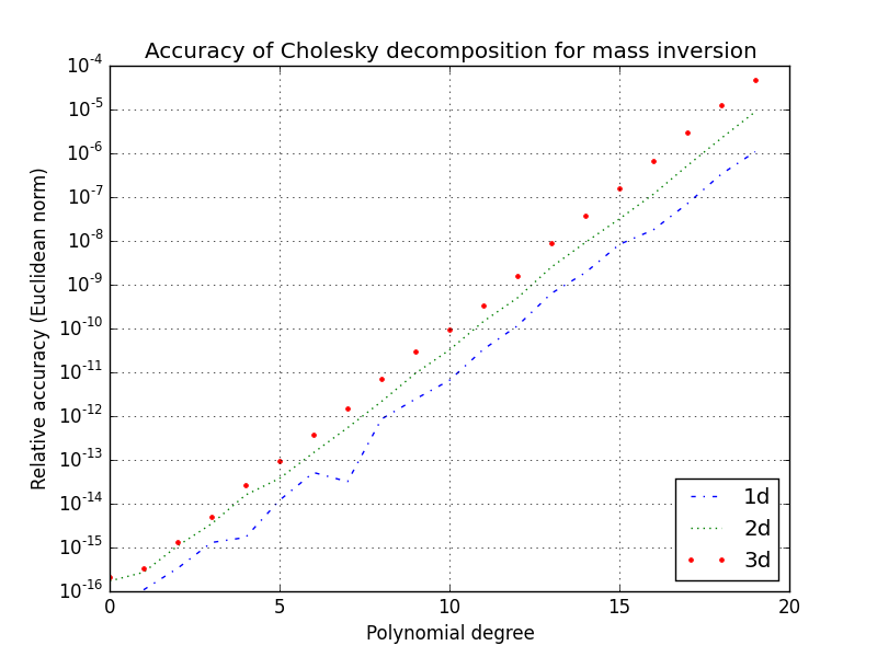
Fig. 1: Relative accuracy of solving linear systems with mass matrices of various degrees using Cholesky decomposition.

Second, we also attempt to solve the linear system using conjugate gradients. We again used systems with random solution, and both letting CG run to a relative residual tolerance of $10^{-12}$ and also stopping after $n+1$ iterations in light of Corollary 4. We display the results of a fixed tolerance in Figure 2. Figure 2(a), shows the actual accuracy obtained for each polynomial degree and Figure 2(b) gives the actual iteration count required. Like Cholesky factorization, this approach gives nearly ten-digit accuracy up to degree ten polynomials. On the other hand, Figure 3 shows that accuracy degrades markedly when only $n+1$ iterations are used.

Finally, our block algorithm gives accuracy comparable to that of Cholesky factorization. Our two-dimensional implementation of Algorithm 2 uses Cholesky factorizations of the one-dimensional mass matrices. Rather than full recursion, our three-dimensional implementation uses Cholesky factorization of the two-dimensional matrices. At any rate, Figure 4 shows, when compared to Figure 1, that we lose very little additional accuracy over Cholesky factorization. Whether replacing the one-dimensional solver with a specialized method for totally positive matrices koev2007accurate would also give high accuracy for the higher-dimensional problems will be the subject of future investigation.

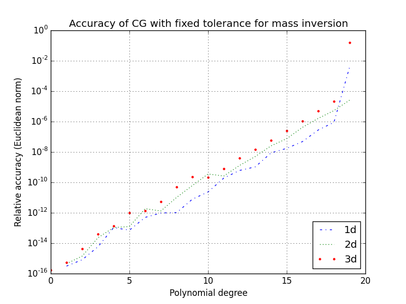
(a) Accuracy obtained by iterating until a residual tolerance of $10^{-12}$.

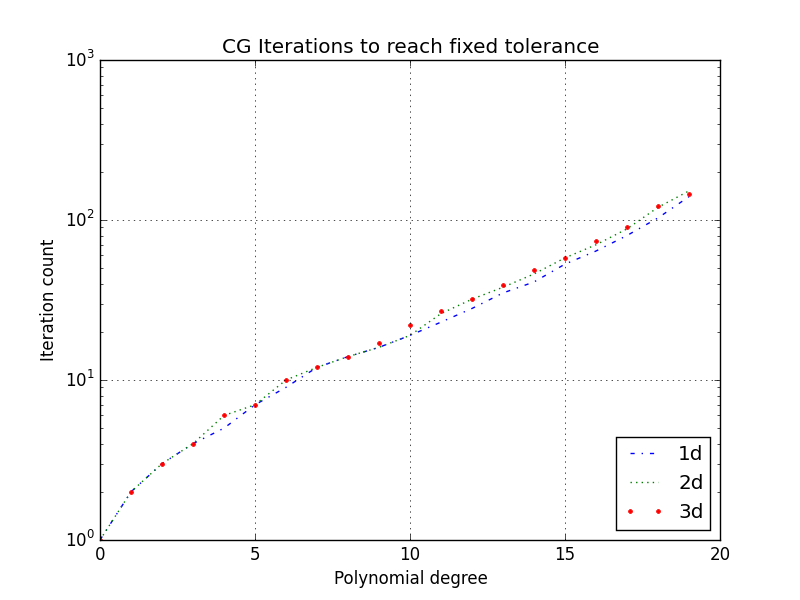
(b) CG iterations required to solve $M^{d,n}x=y$ to a tolerance of $10^{-12}$.

Fig. 2: Accuracy obtained solving mass matrix system using conjugate gradient iteration in one, two, and three space dimensions.

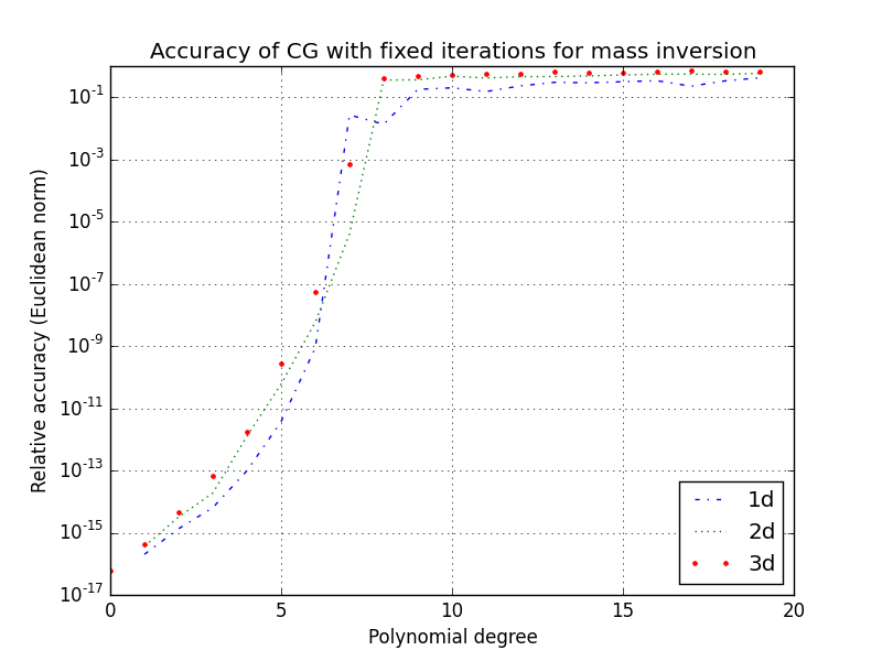
Fig. 3: Relative accuracy of solving $M^{d,n}x=y$ using exactly $n+1$ CG iterations.

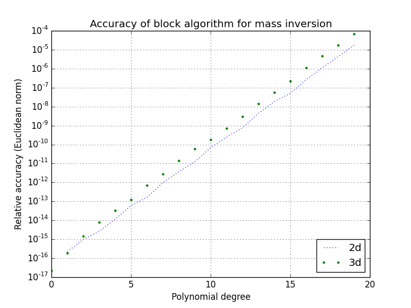
Fig. 4: Relative accuracy of solving linear systems with mass matrices of various degrees using one level of the block algorithm with Cholesky factorization for lower-dimensional matrices.

5.2 Timing for first-order acoustics

We fixed a $32\times 32$ square mesh subdivided into right triangles and computed the time to perform the DG function evaluation (including mass matrix inversion) at various polynomial degrees. We used the mesh from DOLFIN (dolfin, ) and wrote the Bernstein polynomial algorithms in Cython (behnelcython, ). With an $\mathcal{O}(n^{3})$ complexity for two-dimensional problems, we expect a doubling of the polynomial degree to produce an eightfold increase in run-time. In Figure 5, though, we see even better results. In fact, a least-squares fit of the log-log data in this table from degrees five to fifteen gives a very near fit with a slope of less than two (about 1.7) rather than three. Since small calculations tend to run at lower flop rates, it is possible that we are far from the asymptotical regime predicted by our operation counts.

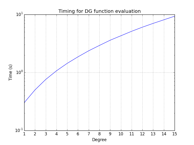
Fig. 5: Timing of a DG function evaluation for various polynomial degrees on a $32\times 32$ mesh.

6 Conclusions and Future Work

Bernstein polynomials admit optimal-complexity algorithms for discontinuous Galerkin methods for conservation laws. The dense element mass matrices might, at first blush, seem to prevent this, but their dimensionally recursive block structure and other interesting properties, lead to an efficient blockwise factorzation. Despite the large condition numbers, our current algorithms seem sufficient to deliver reasonable accuracy at moderate polynomial orders.

On the other hand, these results still leave much room for future investigation. First, it makes sense to explore the possibilities of slope limiting in the Bernstein basis. Second, while our mass inversion algorithm is sufficient for moderate order, it may be possible to construct a different algorithm that maintains the low complexity while giving higher relative accuracy, enabling very high approximation orders. Perhaps such algorithms will either utilize the techniques in (koev2007accurate, ) internally, or else extend them somehow. Finally, our new algorithm, while of optimal compexity, is quite intricate to implement and still is not well-tuned for high performance. Finding ways to make these algorithms more performant will have important practical benefits.

References

- (1) Mark Ainsworth, Gaelle Andriamaro, and Oleg Davydov, Bernstein-Bézier finite elements of arbitrary order and optimal assembly procedures, SIAM Journal on Scientific Computing, 33 (2011), pp. 3087–3109.
- (2) Douglas N. Arnold, Richard S. Falk, and Ragnar Winther, Geometric decompositions and local bases for spaces of finite element differential forms, Computer Methods in Applied Mechanics and Engineering, 198 (2009), pp. 1660–1672.
- (3) Erwin H. Bareiss, Numerical solution of linear equations with Toeplitz and vector Toeplitz matrices, Numerische Mathematik, 13 (1969), pp. 404–424.
- (4) Stephan Behnel, Robert Bradshaw, and Greg Ewing, Cython: C-extensions for python, 2008.
- (5) Susanne C. Brenner and L. Ridgway Scott, The mathematical theory of finite element methods, vol. 15 of Texts in Applied Mathematics, Springer, New York, third ed., 2008.
- (6) Bernardo Cockburn and Chi-Wang Shu, The Runge-Kutta local projection -discontinuous Galerkin finite element method for scalar conservation laws, RAIRO Modél. Math. Anal. Numér, 25 (1991), pp. 337–361.
- (7) Marie-Madeleine Derriennic, On multivariate approximation by Bernstein-type polynomials, Journal of approximation theory, 45 (1985), pp. 155–166.
- (8) Moshe Dubiner, Spectral methods on triangles and other domains, Journal of Scientific Computing, 6 (1991), pp. 345–390.
- (9) Michael G. Duffy, Quadrature over a pyramid or cube of integrands with a singularity at a vertex, SIAM journal on Numerical Analysis, 19 (1982), pp. 1260–1262.
- (10) Michael Dumbser, Dinshaw S. Balsara, Eleuterio F. Toro, and Claus-Dieter Munz, A unified framework for the construction of one-step finite volume and discontinuous Galerkin schemes on unstructured meshes, Journal of Computational Physics, 227 (2008), pp. 8209–8253.
- (11) Rida T. Farouki, Tim N. T. Goodman, and Thomas Sauer, Construction of orthogonal bases for polynomials in Bernstein form on triangular and simplex domains, Computer Aided Geometric Design, 20 (2003), pp. 209–230.
- (12) Sigal Gottlieb, Chi-Wang Shu, and Eitan Tadmor, Strong stability-preserving high-order time discretization methods, SIAM Review, 43 (2001), pp. 89–112.
- (13) Jan S. Hesthaven and Tim Warburton, Nodal high-order methods on unstructured grids: I. time-domain solution of Maxwell’s equations, Journal of Computational Physics, 181 (2002), pp. 186–221.
- (14) , Nodal discontinuous Galerkin methods: algorithms, analysis, and applications, vol. 54, Springer, 2007.
- (15) Hussein Hoteit, Ph. Ackerer, Robert Mosé, Jocelyne Erhel, and Bernard Philippe, New two-dimensional slope limiters for discontinuous Galerkin methods on arbitrary meshes, International journal for numerical methods in engineering, 61 (2004), pp. 2566–2593.
- (16) Eric Jones, Travis Oliphant, and Pearu Peterson, SciPy: Open source scientific tools for Python, http://www. scipy. org/, (2001).
- (17) George Em Karniadakis and Spencer J. Sherwin, Spectral/ element methods for computational fluid dynamics, Numerical Mathematics and Scientific Computation, Oxford University Press, New York, second ed., 2005.
- (18) Robert C. Kirby, Fast simplicial finite element algorithms using Bernstein polynomials, Numerische Mathematik, 117 (2011), pp. 631–652.
- (19) , Low-complexity finite element algorithms for the de Rham complex on simplices, SIAM J. Scientific Computing, 36 (2014), pp. A846–A868.
- (20) Robert C. Kirby and Thinh Tri Kieu, Fast simplicial quadrature-based finite element operators using Bernstein polynomials, Numerische Mathematik, 121 (2012), pp. 261–279.
- (21) Andreas Klöckner, Tim Warburton, Jeff Bridge, and Jan S. Hesthaven, Nodal discontinuous Galerkin methods on graphics processors, Journal of Computational Physics, 228 (2009), pp. 7863–7882.
- (22) Plamen Koev, Accurate computations with totally nonnegative matrices, SIAM Journal on Matrix Analysis and Applications, 29 (2007), pp. 731–751.
- (23) Ming-Jun Lai and Larray L. Schumaker, Spline functions on triangulations, vol. 110 of Encyclopedia of Mathematics and its Applications, Cambridge University Press, Cambridge, 2007.
- (24) Norman Levinson, The Wiener RMS error criterion in filter design and prediction, J. Math. Phys., 25 (1947), pp. 261–278.
- (25) Anders Logg and Garth N. Wells, DOLFIN: automated finite element computing, ACM Trans. Math. Software, 37 (2010), pp. Art. 20, 28.
- (26) G. Andriamaro M. Ainsworth and O. Davydov, A Bernstein-Bezier basis for arbitrary order Raviart-Thomas finite elements, Tech. Report 2012-20, Scientific Computing Group, Brown University, Providence, RI, USA, Oct. 2012. Submitted to Constructive Approximation.
- (27) Chi-Wang Shu, Total-variation-diminishing time discretizations, SIAM Journal on Scientific and Statistical Computing, 9 (1988), pp. 1073–1084.
- (28) Gilbert Strang, Linear algebra and its applications., Belmont, CA: Thomson, Brooks/Cole, 2006.
- (29) A. H. Stroud, Approximate calculation of multiple integrals, Prentice-Hall Inc., Englewood Cliffs, N.J., 1971. Prentice-Hall Series in Automatic Computation.
- (30) Eleuterio F. Toro, Riemann solvers and numerical methods for fluid dynamics, vol. 16, Springer, 1999.
- (31) Tim Warburton, private communication.
- (32) Timothy Warburton, A low-storage curvilinear discontinuous Galerkin method for wave problems, SIAM Journal on Scientific Computing, 35 (2013), pp. A1987–A2012.
- (33) Jun Zhu, Jianxian Qiu, Chi-Wang Shu, and Michael Dumbser, Runge–Kutta discontinuous Galerkin method using WENO limiters II: unstructured meshes, Journal of Computational Physics, 227 (2008), pp. 4330–4353.
- (34) Jun Zhu, Xinghui Zhong, Chi-Wang Shu, and Jianxian Qiu, Runge–Kutta discontinuous Galerkin method using a new type of WENO limiters on unstructured meshes, Journal of Computational Physics, 248 (2013), pp. 200–220.