Three-phase contact line and line tension of electrolyte solutions
in contact with charged substrates

Abstract

The three-phase contact line formed by the intersection of a liquid-vapor interface of an electrolyte solution with a charged planar substrate is studied in terms of classical density functional theory applied to a lattice model. The influence of the substrate charge density and of the ionic strength of the solution on the intrinsic structure of the three-phase contact line and on the corresponding line tension is analyzed. We find a negative line tension for all values of the surface charge density and of the ionic strength considered. The strength of the line tension decreases upon decreasing the contact angle via varying either the temperature or the substrate charge density.

I Introduction

The line tension is the free energy per length associated with the contact line where three phases meet in space. For example, for a sessile liquid drop on a solid substrate and surrounded by the vapor phase, the contact line corresponds to the periphery of the circle where the liquid-vapor interface meets the substrate. Although its magnitude is small (both theoretical and experimental values are of the order of $10^{-12}$ to $10^{-10}$ N Getta1998 ; Qu ; Dobbs ; Schneemilch ; Pompe ; Mugele2002 ; Takata ; Dussaud ; Djikaev ), the line tension plays an important role for various systems and phenomena such as spreading of droplets deGennes ; Fan , wetting of nanoporous surfaces Raspal , stability of emulsions and foams Aveyard , drop size Weijs , and many others. The line tension has been the subject of numerous theoretical and experimental investigations (see, e.g., Refs. SND ; IndekeuLT1 ; IndekeuLT2 ; Rusanov and references therein). Experimental setups to study line tensions encompass solid-liquid-gas systems, such as drops on solid substrates Pompe ; Mugele2002 , bubbles on solid substrates Platikanov ; Rodrigues or on particles at liquid-gas interfaces Scheludko ; Aveyard1995 ; Yakubov , and liquid-liquid-vapor systems, such as liquid lenses at liquid-gas interfaces Takata ; Dussaud ; Aveyard1999 . Theoretical investigations include extensions of capillarity theory Rowlinson , which take into account line tension effects Widom1995 ; Marmur , microscopic theories Tarazona ; Getta1998 ; Bauer ; Weijs2011 ; Zeng2011 , as well as molecular dynamics Bresme1998 ; Bresme1999 ; Werder ; Hirvi ; Schneemilch ; Dutta2011 ; Ramirez2014 and Monte Carlo Djikaev ; Kulmala ; Block simulations. Except for simulations of pure water, these investigations deal with simple fluids or binary liquid mixtures thereof. However, most actual fluids used in wetting applications comprise several components. For polar fluids, such as water, these additional components often carry an ionic character. It is well-known that the presence of ions in a fluid creates the Debye length as an additional length scale, which increases upon decreasing the ionic strength. For dilute electrolyte solutions it typically exceeds the bulk correlation length of the pure solvent. Hence the structure and the wetting behavior of an electrolyte solution can be expected to differ significantly from that of the pure solvent Bier2012 ; Ibagon ; Ibagon2 .

There are only few studies concerned with the influence of electrostatic interactions on the line tension Digilov ; Chou ; Buehrle ; Kang2 ; Kang ; Dorr2014 . In Ref. Digilov the theory of capillarity has been extended taking into account line contributions as well as electric charges at the interfaces and at the three-phase contact line (TPCL). Within this approach electrowetting has been interpreted as a line tension effect, but some of the corresponding predictions are in disagreement with experimental data Quilliet . In Ref. Chou an equation for the contact angle as function of the electrostatic potential at the TPCL and an estimate for the electrostatic contribution to the line tension have been derived using a variational approach for a wedge-like geometry. Based on a Poisson-Boltzmann theory the analysis in Refs. Kang ; Kang2 considers only the electrostatic part of the free energy. Therefore, only the electrostatic contribution to the line tension is analyzed. The density distribution of a conductive liquid close to the three-phase contact line has been calculated numerically in Ref. Buehrle , but the line tension was not studied. Recently, Dörr and Hardt Dorr studied the electric double layer structure close to the TPCL by solving the linearized Poisson-Boltzmann equation in a wedge geometry, without calculating the line tension. Following the method used in Ref. Dorr , Das and Mitra calculated the Maxwell stress and the contact angle of drops or bubbles on a charged substrate, again without taking into account line effects Das . More recently, Dörr and Hardt Dorr2014 computed the line tension of an electrolyte in contact with a charged substrate by considering a wedge geometry similar to Refs. Kang ; Kang2 ; Dorr ; Das . Similarly to Refs. Kang ; Kang2 , they considered only the electrostatic contribution to the line tension. However, their model differs from the one in Refs. Kang ; Kang2 in that it incorporates the deformation of the fluid-fluid interface near the TPCL relative to planar shapes. To our knowledge there are no microscopic calculations of line tensions in electrolyte solutions in which both solvent and ion contributions are taken into account simultaneously.

Here we present a microscopic calculation of the line tension and of the intrinsic TPCL structure for a lattice model of an electrolyte solution in contact with a charged substrate which takes into account solvent and ion contributions via classical density functional theory. The wetting phenomena of this model have already been studied in Ref. Ibagon . In Sec. II we recall this model and the corresponding density functional. The results for the line tension and the TPCL structure for both the salt-free solvent and the electrolyte solutions are discussed in Sec. III. We conclude and summarize our main results in Sec. IV.

II Model and density functional theory

II.1 Model

We study a semi-infinite lattice model for an electrolyte solution in contact with a charged wall. This model is the same as the one used in Ref. Ibagon . It consists of three components: solvent $(0)$, anions $(-)$, and cations $(+)$. The $z$ axis is perpendicular to the wall. The region above the wall, which is the one accessible to the electrolyte components, is divided into a set of cells the centers of which form a simple cubic lattice $\{\bf r\}$ with lattice constant $a$. The volume $a^{3}$ of such a cell corresponds roughly to the volumina of the particles, which are assumed to be of similar size. The centers of the molecules in the top layer of the substrate form the plane $z=0$. At closest approach the centers of the solvent molecules and ions are at $z=a$. The plane $z=a/2$ is taken to be the surface of the planar wall. Each cell is either empty or occupied by a single particle. This mimics the steric hard core repulsion between all particles. Particles at different sites interact among each other via an attractive nearest-neighbor interaction of strength $u$ which is taken to be the same for all pairs of particles. In addition, ion pairs interact via the Coulomb potential.

The wall attracts particles only in the first adjacent layer via an interaction potential of strength $u_{\text{w}}$ which is the same for all species. In addition it can carry a surface charge density $\tilde{\sigma}=\sigma ea^{-2}$ which is taken to be localized in the plane $z=a/2$ and which interacts electrostatically with the ions; $e>0$ is the elementary charge. The surface charge density $\tilde{\sigma}$ is assumed to be laterally uniform and independent of the structure of the adjacent fluid, i.e., it is the same for a liquid-wall and for a gas-wall interface. This situation is typically realized in EWOD (electrowetting on dielectrics) setups Berge1993 ; Mugele2005 , in which the wall is composed of an electrode covered by a micron-sized isolating dielectric layer. For these systems the areal wall charge density is determined by the laterally uniform capacity of the dielectric layer and not by charge-regulation mechanisms or by the electric double layer structure in the electrolyte solution.

For the present model it is known Ibagon that in the presence of ions a first-order wetting transition occurs to which a prewetting line is attached from which layering transition lines depart towards higher temperatures (see Fig. 7 in Ref. Ibagon ). These latter artifacts due to the lattice model used here are not expected to influence the results below because in the following only bulk states at liquid-vapor coexistence below the wetting transition are considered.

II.2 Density functional

We denote the dimensionless lattice positions as ${\bf\bar{r}}={\bf r}/a$ and $\tilde{\rho}_{i}({\bf\bar{r}})=\rho_{i}({\bf\bar{r}})a^{-3}$ with $i\in\{0,+,-\}$ denotes the number densities of the solvent ($i=0$) and of the $\pm$-ions. The equilibrium profiles $\rho_{0}$, $\rho_{+}$, and $\rho_{-}$ minimize the following grand canonical density functional:

$$\begin{split}\beta\Omega\left[\{\rho_{i}({\bf\bar{r}})\}\right]&=\sum_{{\bf\bar{r}}}\left[\sum_{i}\rho_{i}({\bf\bar{r}})\ln{\rho_{i}({\bf\bar{r}})}\right.\\ &\left.+\Big{(}1-\sum_{i}\rho_{i}({\bf\bar{r}})\Big{)}\ln{\Big{(}1-\sum_{j}\rho_{j}({\bf\bar{r}})\Big{)}}\right]\\ &+\frac{1}{2}\beta\sum_{\begin{subarray}{c}{\bf\bar{r}},{\bf\bar{r}^{\prime}}\\ {\bf\bar{r}}\neq{\bf\bar{r}^{\prime}}\end{subarray}}\sum_{i,j}\rho_{i}({\bf\bar{r}})\rho_{j}({\bf\bar{r}^{\prime}})w\left(|{\bf\bar{r}}-{\bf\bar{r}^{\prime}}|\right)\\ &-\beta\sum_{{\bf\bar{r}}}\sum_{i}u_{\text{w}}\delta_{\bar{z},1}\rho_{i}({\bf\bar{r}})-\beta\sum_{{\bf\bar{r}}}\sum_{i}\mu_{i}\rho_{i}({\bf\bar{r}})\\ &+2\pi l_{B}\int_{V}\!d^{3}\bar{r}^{*}\frac{\left({\bf D}\left({\bf\bar{r}^{*}},[\rho^{*}_{\pm}]\right)\right)^{2}}{\varepsilon(\rho^{*}_{0}({\bf\bar{r}^{*}}))},\end{split}$$ (1)

where $\beta=(k_{B}T)^{-1}$ is the inverse thermal energy; $\mu_{i}$ is the chemical potential of species $i$; $\tilde{l}_{B}=l_{B}a=e^{2}\beta/(4\pi\varepsilon_{0})$ is the Bjerrum length in vacuum; and ${\bf\bar{r}^{*}}={\bf r^{*}}/a$, $\rho^{*}_{i}({\bf\bar{r}^{*}})=\rho_{i}({\bf\bar{r}})$ for all ${\bf\bar{r}^{*}}\in\mathbb{R}^{3}$ and ${\bf\bar{r}}\in\mathbb{Z}^{3}$ with $\max\left(|\bar{x}^{*}-\bar{x}|,|\bar{y}^{*}-\bar{y}|,|\bar{z}^{*}-\bar{z}|\right)\leq 1/2$, i.e., with ${\bf\bar{r}}$ corresponding to that site of the discrete cubic lattice $\mathbb{Z}^{3}$ being located closest to position ${\bf\bar{r}^{*}}$ in the continuous space $\mathbb{R}^{3}$. The pair potential common for all species is $w\left(|{\bf r}-{\bf r^{\prime}}|\right)=-u$ for nearest neighbors (i.e., $u>0$ corresponds to attraction) and $w\left(|{\bf r}-{\bf r^{\prime}}|\right)=0$ beyond; $-u_{\text{w}}$ is the strength of the attractive ($u_{\text{w}}>0$) substrate potential acting on the first layer $z=a$. $\tilde{\bf D}={\bf D}ea^{-2}$ is the actual electric displacement generated by the ions and the surface charge density $\tilde{\sigma}=\sigma ea^{-2}$, satisfying Gauß’s law Jackson with the dimensionless gradient $\nabla$ obtained by rescaling with $a$:

$$\nabla\cdot{\bf D}\left({\bf\bar{r}^{*}},[\rho^{*}_{\pm}]\right)=\sum_{i}q_{i}\rho^{*}_{i}({\bf\bar{r}^{*}})+\sigma\delta(\bar{z}-1/2);$$ (2)

The concept underlying this form of Gauß’s law is that all microscopic charges besides the ionic monopoles and the surface charges, e.g., those due to permanent or induced dipoles, are implicitly accounted for in terms of the relative permittivity $\varepsilon(\rho^{*}_{0}({\bf\bar{r}^{*}}))$. Here the relative permittivity is assumed to be dominated by the solvent properties, as it is the case for polar solvents such as water, so that it depends only on the solvent density $\rho_{0}({\bf\bar{r}})$ but not on the ion densities $\rho_{\pm}({\bf\bar{r}})$.

The description in Eq. (1) does not account for the structure of a hydration shell, neither in the bulk nor at interfaces. For actual systems there is a strong dependence of, e.g., the value of the interfacial tension of a liquid-vapor interface on atomistic details of ion hydration Tobias2013 ; but it is not the aim of the present study to model such details. Moreover, here the solubility of ions is accounted for merely effectively via the ion-solvent interaction $w\left(|{\bf\bar{r}}-{\bf\bar{r}^{\prime}}|\right)$, which, for the sake of simplicity, is the same between all particle species. More realistic descriptions could be used instead, e.g., in terms of the Born energy Born1920 , but this is not done here for reasons of simplicity.

The bulk phase diagram, i.e., the solvent and the $\pm$-ion densities in the liquid ($\{\rho_{i,l}\}$) and in the gas phase ($\{\rho_{i,g}\}$) of the solution, has already been determined in Ref. Ibagon . The bulk equilibrium densities are calculated by minimizing the bulk grand canonical potential

$$\frac{\beta\Omega[\{\rho_{i}\}]}{\bar{V}}=\rho_{0}(\ln{\rho_{0}}-\mu^{*}_{0})+I(2\ln{I}-\mu^{*}_{I})\\ +(1-\rho_{0}-2I)\ln{(1-\rho_{0}-2I)}-\frac{1}{T^{*}}(\rho_{0}+2I)^{2},$$ (3)

where $I:=\rho_{+}=\rho_{-}$ (due to local charge neutrality) is the so-called ionic strength for monovalent ions; $\mu^{*}_{0}=\beta\mu_{0}$, $\mu^{*}_{I}=\beta(\mu_{+}+\mu_{-})$, $T^{*}=\frac{1}{3\beta u}$ is the reduced temperature, and $V=\bar{V}a^{3}$ is the volume of the fluid. The last term in Eq. (1) vanishes because in the bulk $\mathbf{D}=0$ due to Eq. (2). For $I=0$, the reduced critical temperature is $T^{*}_{c}(I=0)=0.5$ and the critical number density of the solvent is $\rho_{0,c}(I=0)=0.5$. For $I\neq 0$, the reduced critical temperature $T^{*}_{c}$ is independent of $I$ whereas $\rho_{0,c}(I)=0.5-2I$ Ibagon .

At two-phase coexistence for temperatures below the critical point, $T^{*}\leq T^{*}_{c}$, the bulk densities $\{\rho_{i,l}\}$ in the liquid and $\{\rho_{i,g}\}$ in the gas phase are fully specified by the four values $\rho_{0,l}$, $I_{l}$, $\rho_{0,g}$, and $I_{g}$, which have to fulfill the three coexistence conditions (see Eq. (26) of Ref. Ibagon )

$$\mu_{0}[\{\rho_{i,l}\},T^{*}] =\mu_{0}[\{\rho_{i,g}\},T^{*}],$$

$$\mu_{I}[\{\rho_{i,l}\},T^{*}] =\mu_{I}[\{\rho_{i,g}\},T^{*}],$$

$$p[\{\rho_{i,l}\},T^{*}] =p[\{\rho_{i,g}\},T^{*}],$$ (4)

where $p=-\Omega/V$ is the pressure. Hence, in addition to Eq. (4), one of the four values $\rho_{0,l},I_{l},\rho_{0,g},I_{g}$ can be fixed arbitrarily; in the following we choose the ionic strength in the liquid, $I_{l}$, which, is simply called the ionic strength $I$ in Sec. III.

With the bulk properties fixed and with a given expression for the relative permittivity $\varepsilon(\rho^{*}_{0}({\bf\bar{r}^{*}}))$, the functional in Eq. (1) can be used to study the wetting behavior of electrolyte solutions as it has been done in Ref. Ibagon . If the substrate potential depends only on the direction $\bar{z}$ perpendicular to the wall and if the boundary condition for $\bar{z}\to\infty$ is laterally homogeneous, the equilibrium density profiles depend on $\bar{z}$ only but not on $\bar{x}$ or $\bar{y}$. Accordingly the grand canonical functional in Eq. (1) decomposes into the bulk contribution given by Eq. (3) and into a surface contribution proportional to the area $A=\bar{A}a^{2}$ of the substrate:

$$\Omega\left[\{\rho_{i}({\bf\bar{r}})\}\right]=V\Omega_{b}[\rho_{i}]+A\Omega_{s}[\{\rho_{i}(\bar{z})\}].$$ (5)

The substrate-liquid surface tension $\gamma_{s,l}$ and the substrate-gas surface tension $\gamma_{s,g}$ are given by

$$\gamma_{s,l}=\min_{\{\rho_{i}(\bar{z})\}}{\Omega_{s}[\{\rho_{i}(\bar{z})\}]},\ \ \ \ \text{for}\ \rho_{i}(z\to\infty)=\rho_{i,l},$$ (6)

and

$$\gamma_{s,g}=\min_{\{\rho_{i}(\bar{z})\}}{\Omega_{s}[\{\rho_{i}(\bar{z})\}]},\ \ \ \ \text{for}\ \rho_{i}(z\to\infty)=\rho_{i,g},$$ (7)

respectively. The equilibrium density profiles which minimize Eq. (6) correspond to the substrate-liquid interface, while the ones which minimize Eq. (7) correspond to the substrate-gas interface, which consists of the emerging substrate-liquid and liquid-gas interfaces separated by a liquid-like layer of thickness $\tilde{\ell}_{0}(T)=a\ell_{0}(T)$. At two-phase coexistence, i.e., for $\mu^{*}_{i}=\mu^{*}_{i,co}$, both density profiles described above are equilibrium density distributions.

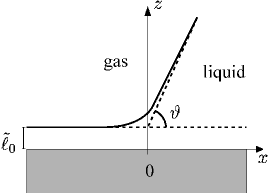
Figure 1: Generic shape $z=\tilde{\ell}(x)$ of the liquid-gas interface (full line) near the three-phase contact line (TPCL) on a homogeneous planar surface; $\tilde{\ell}_{0}$ is the equilibrium thickness of the microscopicly thin liquid-like film for $T$ below the wetting transition temperature $T_{\text{w}}$ and at two-phase coexistence. The dashed lines represent the asymptotes of $z=\tilde{\ell}(x)$ for $x\to\infty$ and $x\to-\infty$. The position $x=0$ is defined as the point at which the asymptotes intersect. The asymptote $z=\tilde{\ell}(x\to\infty)$ intersects the substrate with the contact angle $\vartheta$. The density distribution is translationally invariant along the $y$ direction perpendicular to the $x$-$z$-plane.

Imposing these two distinct boundary conditions at $\bar{x}=\pm\infty$ for $\bar{z}\to\infty$, i.e., $\rho_{i}(\bar{x}\to\infty,\bar{z}\to\infty)=\rho_{i,l}$ and $\rho_{i}(\bar{x}\to-\infty,\bar{z}\to\infty)=\rho_{i,g}$, the minimization of Eq. (1) leads to an equilibrium density distribution $\rho_{i}(\bar{x},\bar{z})$ which interpolates smoothly between a substrate-gas interface at $\bar{x}\to-\infty$ and a substrate-liquid interface at $\bar{x}\to+\infty$. A specific definition of the local position of the liquid-gas interface renders a curve $\bar{z}=\ell(\bar{x})$ (see, c.f., Eq. (16)) such that $\ell(\bar{x}\to-\infty)=\ell_{0}(T)$ and $\ell(\bar{x}\to\infty)=\ell_{0}(T)+\bar{x}\tan\vartheta$, where $\vartheta$ is the contact angle (see Fig. 1). This arrangement leads to the formation of a straight TPCL independent of $\bar{y}$ where the liquid-gas, the substrate-gas, and the substrate-liquid interfaces intersect.

For $\rho_{i}({\bf\bar{r}})=\rho_{i}(\bar{x},\bar{z})$, the density functional in Eq. (1) can be written as

$$\begin{split}\frac{\beta\Omega\left[\{\rho_{i}(\bar{x},\bar{z})\}\right]}{\bar{L}}&=\mkern-18.0mu\sum_{\bar{x}=-n_{x}}^{n_{x}}\sum_{\bar{z}=1}^{\bar{L}_{z}}\left\{\sum_{i}\rho_{i}(\bar{z})\ln{\rho_{i}(\bar{x},\bar{z})}+\Big{(}1-\sum_{i}\rho_{i}(\bar{x},\bar{z})\Big{)}\ln{\Big{(}1-\sum_{j}\rho_{j}(\bar{x},\bar{z})\Big{)}}\right.\\ &\phantom{=}-\frac{\beta u}{2}\sum_{ij}\rho_{i}(\bar{x},\bar{z})\left(\rho_{j}(\bar{x}\!+\!1,\bar{z})+\rho_{j}(\bar{x}\!-\!1,\bar{z})+\rho_{j}(\bar{x},\bar{z}\!+\!1)\right.\\ &\phantom{=}\left.\left.+\rho_{j}(\bar{x},\bar{z}\!-\!1)+2\rho_{j}(\bar{x},\bar{z})\right)-\beta u_{\text{w}}\sum_{i}\rho_{i}(\bar{x},\bar{z})\delta_{\bar{z},1}-\beta\sum_{i}\mu_{i}\rho_{i}(\bar{x},\bar{z})\right\}\\ &\phantom{=}+2\pi l_{B}\int_{-\bar{L}_{x}/2}^{\bar{L}_{x}/2}\int_{1/2}^{\bar{L}_{z}+1/2}\!d\bar{x}^{*}d\bar{z}^{*}\frac{\left(\mathbf{D}(\bar{x}^{*},\bar{z}^{*},[\rho^{*}_{\pm}])\right)^{2}}{\varepsilon(\rho^{*}_{0}(\bar{x},\bar{z}))},\end{split}$$ (8)

where $n_{x}=\frac{\bar{L}_{x}-1}{2}$ with lateral system size $\bar{L}_{x}$, $\bar{L}=L/a$ is the contact line length in the invariant $\bar{y}$ direction, and the fluid volume is $V=L_{x}L_{z}L$; $i,j=0,+,-$.

Gauß’s law (Eq. 2) can be written as

$$\nabla\cdot{\bf D}\left({\bar{x}^{*},\bar{z}^{*}},[\rho^{*}_{\pm}]\right)=\sum_{i}q_{i}\rho^{*}_{i}(\bar{x}^{*},\bar{z}^{*}).$$ (9)

with the boundary conditions

$$\left.D_{z}(\bar{x}^{*},\bar{z}^{*},[\rho^{*}_{\pm}])\right|_{\bar{z}^{*}=1/2} =\sigma,$$ (10)

$$\left.D_{z}(\bar{x}^{*},\bar{z}^{*},[\rho^{*}_{\pm}])\right|_{\bar{z}^{*}=\bar{L}_{z}+1/2} =0,$$

$$\left.D_{x}(\bar{x}^{*},\bar{z}^{*},[\rho^{*}_{\pm}])\right|_{\bar{x}^{*}=-\bar{L}_{x}/2} =0,$$

$$\left.D_{x}(\bar{x}^{*},\bar{z}^{*},[\rho^{*}_{\pm}])\right|_{\bar{x}^{*}=\bar{L}_{x}/2} =0,$$

which follow from the overall charge neutrality.

The relative permittivity $\varepsilon(\bar{z}^{*})$ is taken to depend locally on the solvent density $\rho^{*}_{0}(\bar{x}^{*},\bar{z}^{*})$ through the Clausius-Mossotti expression Jackson

$$\varepsilon(\rho^{*}_{0}(\bar{x}^{*},\bar{z}^{*}))=\frac{1+\frac{2\alpha}{3\varepsilon_{0}}\rho^{*}_{0}(\bar{x}^{*},\bar{z}^{*})}{1-\frac{\alpha}{3\varepsilon_{0}}\rho^{*}_{0}(\bar{x}^{*},\bar{z}^{*})},$$ (11)

where $\alpha$ is an effective polarizability of the solvent molecules. In the following its value is chosen such that $\varepsilon=60$ for $\rho_{0}=1$; this choice corresponds to a mean value for liquid water along the liquid-gas coexistence curve. It is well-known that the Clausius-Mossotti relation between the relative permittivity $\varepsilon$ and the polarizability $\alpha$ holds only for dilute gases. However, Eq. (11) is merely used as a simple functional form in order to obtain the dependence on $\rho^{*}_{0}$ of the relative permittivity with $\alpha$ being a fitting parameter which is adapted to interpolate between $\varepsilon(\rho^{*}_{0})\to 1$ for $\rho^{*}_{0}\to 0$ and a large value (here $\varepsilon(\rho^{*}_{0})\to 60$) for $\rho^{*}_{0}\to 1$.

The Euler-Lagrange equations, which follow from the minimization of Eq. (8) analogously to the procedure presented in Subsec. IIC in Ref. Ibagon , are given by

$$\ln{\rho_{i}(\bar{x},\bar{z})}-\mu^{*}_{i}-\beta u_{\text{w}}\delta_{\bar{z},1}-\ln{\Big{(}1-\sum_{j}\rho_{j}(\bar{x},\bar{z})\Big{)}}\\ -\frac{1}{3T^{*}}\sum_{j}\left(2\rho_{j}(\bar{x},\bar{z})+\rho_{j}(\bar{x}+1,\bar{z})+\rho_{j}(\bar{x}-1,\bar{z})+\rho_{j}(\bar{x},\bar{z}+1)+\rho_{j}(\bar{x},\bar{z}-1)\right)\\ +q_{i}\int_{\bar{z}-1/2}^{\bar{z}+1/2}\!d\bar{z}^{*}\phi(\bar{x}^{*},\bar{z}^{*})-2\pi l_{B}\int_{\bar{z}-1/2}^{\bar{z}+1/2}\!d\bar{z}^{*}\frac{\left(\mathbf{D}(\bar{x}^{*},\bar{z}^{*},[\rho^{*}_{\pm}])\right)^{2}}{\left(\varepsilon(\rho^{*}_{0}(\bar{x}^{*},\bar{z}^{*}))\right)^{2}}\varepsilon^{\prime}\left(\rho^{*}_{0}(\bar{x}^{*},\bar{z}^{*})\right)\delta_{i,0}=0,$$ (12)

with $i,j=0,+,-$, where $q_{i}e$ is the electric charge of component $i$, $T^{*}=\frac{1}{3\beta u}$ is the reduced temperature and $\mu^{*}_{i}=\beta\mu_{i}$. $\phi(\bar{x}^{*},\bar{z}^{*})=\beta e\tilde{\phi}(x^{*},z^{*})$ is the dimensionless electrostatic potential which fulfills

$$\mathbf{D}(\bar{x}^{*},\bar{z}^{*})=-\frac{\varepsilon}{4\pi l_{B}}\nabla\phi(\bar{x}^{*},\bar{z}^{*}).$$ (13)

At the wall the convention $\rho_{j}(\bar{x},0)=0$ is used.

For given chemical potentials $\mu_{i,co}$ at coexistence, the coupled equations in Eq. (12) are solved for $\{\rho_{i}(\bar{x},\bar{z})\}$ numerically by applying a Picard iteration scheme. The electrostatic potential $\phi(\bar{x}^{*},\bar{z}^{*})$ is calculated for each iteration step by solving Poisson’s equation

$$\nabla\cdot\left(\varepsilon(\rho^{*}_{0}(\bar{x}^{*},\bar{z}^{*}))\nabla\phi(\bar{x}^{*},\bar{z}^{*})\right)=-4\pi l_{B}\sum_{i}q_{i}\rho_{i}^{*}(\bar{x}^{*},\bar{z}^{*}),$$ (14)

which is a nonlinear integro-differential equation for $\phi$ after eliminating $\rho_{\pm}^{*}(\bar{x}^{*},\bar{z}^{*})$ by means of Eq. (12).

II.3 Line tension calculation

The line tension $\tau$ is calculated from the equilibrium density profiles $\{\rho_{i}(\bar{x},\bar{z})\}$ using the following definition for $\tau$:

$$\Omega=\sum_{\alpha=g,l}V_{\alpha}\Omega_{\alpha}+A_{s,g}\gamma_{s,g}+A_{s,l}\gamma_{s,l}+A_{l,g}\gamma_{l,g}+\tau L+\cdots,$$ (15)

where $V_{\alpha}$ is the volume of phase $\alpha$ with $\alpha\in\{g,l\}$ and $\Omega_{\alpha}$ is the bulk free energy density of this phase; $\gamma_{s,g}$, $\gamma_{s,l}$, and $\gamma_{l,g}$ are the interfacial tensions and $A_{s,g}$, $A_{s,l}$, and $A_{l,g}$ the corresponding interfacial areas of the substrate-gas, substrate-liquid, and liquid-gas interfaces, respectively. $L$ is the length of the three-phase contact line, $\tau$ is the line tension and $\cdots$ denotes subleading terms which vanish for macroscopically long contact lines $L\to\infty$.

The plane $\bar{z}=0$ is chosen as the substrate-fluid dividing interface. In Ref. SND it has been proposed that in order to determine the line tension $\tau$ unambiguously from microscopic calculations in a finite box, its boundaries have to be chosen such that the interfaces are cut perpendicularly and that its edges are placed inside the homogeneous regions of the system. Here, in order to calculate the line tension, the integration box proposed in Ref. SND has been used (see Fig. 7 in Ref. SND and, c.f., Fig. 12). However, in a lattice model this type of box introduces technical difficulties for the integration procedure which lead to numerical errors (see Appendix A for more details). Therefore, in order to verify the consistency of the results, the line tension has been calculated for various sizes of the integration box as described in Appendix A.

II.4 Choice of parameters

The values of the parameters used here are the same as the ones used in Ref. Ibagon . The lattice constant $a$ is chosen to be equal to $4\,\text{\AA}$, so that the maximal density $1/a^{3}$ lies between the number densities for liquid water at the triple point and at the critical point. Accordingly, the choice $l_{B}=100$ corresponds to $T\approx 417\,\text{K}$. This temperature lies between the triple point temperature of $273\,\text{K}$ and the critical point temperature of $647\,\text{K}$ for water. In our units $1\,\text{mM}=10^{-3}\,\text{mol}/\text{liter}$ corresponds to $\rho_{i}=\tilde{\rho}_{i}a^{3}=3.9\times 10^{-5}$. The values for the reduced surface charge density $\sigma$ are in the range between 0 and $10^{-2}$. For $a=4\,\text{\AA}$ the latter value corresponds to $1\,\mu\text{C}/\text{cm}^{2}$, which can be achieved for an EWOD setup (see Sec. II.1) by applying the moderate voltage of $60\,\text{V}$ across a $100\,\text{nm}$ thick isolating dielectric layer with a typical dielectric constant $\epsilon_{\text{layer}}=2$. In these units $\beta\tau a=0.1$ corresponds to $\tau\approx 1.4\times 10^{-12}$ N.

III Structure of the three-phase contact line and line tension

III.1 Line tension of the pure solvent

Figure 2: Local positions of the liquid-gas interface for two temperatures with $u_{\text{w}}/u=0.69$ for the pure solvent. The system undergoes a second-order wetting transition at $T^{*}_{\text{w}}\simeq 0.95\times T^{*}_{c}$ (see Fig. 2(b) in Ref. Ibagon ). The positions of the liquid-gas interfaces $\bar{z}=\ell(\bar{x})$ (full lines) have been calculated from the density profiles $\rho_{0}(\bar{x},\bar{z})$ according to Eq. (16). For both $\bar{x}\to\infty$ and $\bar{x}\to-\infty$, the curve $\bar{z}=\ell(\bar{x})$ approaches the asymptotes (dashed lines) from above. The position $\bar{x}=0$ is defined as the point at which the asymptotes intersect.

First, we consider the case $I=0$. As explained in Refs. Pandit1982 ; Pandit1983 ; Ibagon , in this case the ratio $u_{\text{w}}/u=3T^{*}\beta u_{\text{w}}$ controls the wetting and drying transitions. For $u_{\text{w}}/u>1$ the substrate is so strong that it is already wet at $T^{*}=0$; within the range $0.5<u_{\text{w}}/u<1$ there is a wetting transition at $T^{*}_{\text{w}}>0$; and within the parameter range $0\leq u_{\text{w}}/u<0.5$ a drying transition occurs. Here, the liquid-gas interfaces near the TPCL and the line tension are studied for the specific choice $u_{\text{w}}/u=0.69$, for which the system undergoes a second-order wetting transition (see Fig. 2(b) in Ref. Ibagon ) at $T^{*}_{\text{w}}\simeq 0.95T^{*}_{c}$. We note that second-order wetting transitions in a pure solvent with short-ranged interactions is not very realistic as most wetting transitions either are of first order (due to weak van der Waals interactions) or comprise a first-order thin-thick transition followed by a second-order wetting transition (due to strong van der Waals interactions) Bonn2009 . However, the order of wetting transitions of the pure solvent is not important here; instead we intend to exploit the technical advantages offered by short-ranged interactions for the present study.

Figure 2 shows the temperature dependence of the shape $\ell(\bar{x})$ of the local liquid-gas interface position defined as

$$\ell(\bar{x})=\frac{\displaystyle\sum_{\bar{z}=1}^{\bar{L}_{z}}\left(\rho_{0}(\bar{x},\bar{z})-\rho_{0,g}\right)}{\rho_{0,l}-\rho_{0,g}}.$$ (16)

In the case of second-order wetting transitions, the curve $\bar{z}=\ell(\bar{x})$ approaches the asymptotes for $\bar{x}\to\infty$ and $\bar{x}\to-\infty$ from above (Fig. 2). This result is in qualitative agreement with previous ones also obtained in the presence of second-order wetting transitions IndekeuLT1 ; Getta1998 ; Bauer ; Merath .

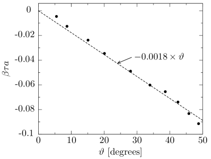
Figure 3: Dependence of the line tension $\tau$ on the contact angle for the same pure system as in Fig. 2. The numerical results for the line tension ($\bullet$) are consistent with the predictions of Ref. IndekeuLT1 for systems exhibiting second-order wetting transitions with short-ranged interactions, i.e., $\tau$ is negative and for $\vartheta\to 0$ it vanishes as $\tau\sim-\vartheta$. The uncertainty of the line tension values corresponds approximately to the size of the symbols. The dashed line is a fit. For details concerning the calculation of the line tension see Appendix A.

The line tension as a function of the contact angle $\vartheta$ is presented in Fig. 3. The contact angle has been changed by varying the temperature $T^{*}$. The results for the line tension are compatible with the prediction of the interface displacement model (IDM) IndekeuLT1 for a system with short-ranged interactions approaching a second-order wetting transition at two-phase coexistence. In this case, the line tension $\tau$ is negative and vanishes as $\tau\sim-\vartheta$. The order of magnitude of $\beta\tau a\approx 0.1$, which corresponds to $\tau\approx 1.4\times 10^{-12}$ N, is comparable also with values obtained from other theoretical approaches for one-component, charge-free fluids Getta1998 ; Qu ; Dobbs and from computer simulations Djikaev ; Schneemilch as well as with experimental results Dussaud ; Pompe ; Mugele2002 ; Takata .

III.2 Line tension of an electrolyte solution

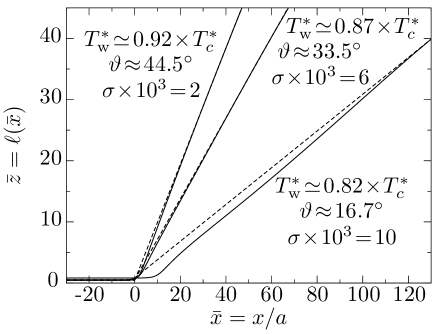
Figure 4: Shapes of liquid-gas interfaces for an electrolyte solution, which exhibits a first-order wetting transition, for various surface charge densities $\tilde{\sigma}=\sigma ea^{-2}$, fixed temperature $T^{*}=0.8\times T^{*}_{c}$, $u_{\text{w}}/u=0.69$, and fixed $I=3.9\times 10^{-5}$ ($\tilde{I}=1\,$mM). Note that for the electrolyte solution the wetting temperature $T_{\text{w}}$ depends on the surface charge density (see Fig. 5 in Ref. Ibagon ). The shapes $\ell(\bar{x})$ (full lines) have been obtained from the density profiles $\rho_{0}(\bar{x},\bar{z})$ using Eq. (16). For first-order wetting, the local interface position $\bar{z}=\ell(\bar{x})$ approach their asymptotes (dashed lines) from above for $\bar{x}\to-\infty$ and from below for $\bar{x}\to\infty$. The position $\bar{x}=0$ is defined as the point at which the pair of asymptotes intersect.

In this section we study the influence of the ionic strength $\tilde{I}=Ia^{-3}$ and of the surface charge density $\tilde{\sigma}=\sigma ea^{-2}$ on the TPCL and the line tension. As discussed in Refs. Ibagon ; Ibagon2 , within the chosen lattice model for an electrolyte solution, if $\sigma\neq 0$ and $I\neq 0$ the system undergoes a first-order wetting transition, irrespective of the order of the wetting transition of the pure solvent. In this case, the wetting transition temperature $T^{*}_{\text{w}}$ decreases with increasing surface charge density $\sigma$ of the substrate for fixed ionic strength $I$ or with decreasing ionic strength $I$ for fixed surface charge density $\sigma$. Therefore, there are three different routes to vary the contact angle: (i) changing the reduced temperature $T^{*}$ and keeping the surface charge density $\sigma$ and the ionic strength $I$ fixed; (ii) changing the surface charge density of the substrate $\sigma$ and keeping the temperature $T^{*}$ and the ionic strength $I$ fixed; and (iii) changing the ionic strength $I$ and keeping the temperature $T^{*}$ and the surface charge density $\sigma$ fixed. Here we consider the routes (i) and (ii) for two values of the ionic strength: $I=3.9\times 10^{-5}$ ($\tilde{I}=1$mM) and $I=3.9\times 10^{-4}$ ($\tilde{I}=10$mM) with $u_{\text{w}}/u=0.69$.

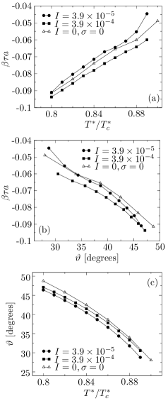
Figure 5: Line tension $\tau$ as a function of temperature $T^{*}$ (a) and of the contact angle $\vartheta$ (b) for $\sigma=1\times 10^{-3}$ and $u_{\text{w}}/u=0.69$. The two types of full symbols correspond to distinct values of the ionic strength $I=\tilde{I}a^{3}$ in the bulk liquid phase ($\bullet$ for $I=3.9\times 10^{-5}$ ($\tilde{I}=1$mM) and $\scriptstyle\blacksquare$ for $I=3.9\times 10^{-4}$ ($\tilde{I}=10$mM)); the uncertainty of the line tension values corresponds approximately to the size of the symbols. For constant $\sigma$ and $T^{*}$, the strength $|\tau|$ of the (negative) line tension $\tau$ increases upon increasing the ionic strength $I$ (see $\bullet$ and $\scriptstyle\blacksquare$ in panel (a)). The open triangles $\vartriangle$ correspond to the case $I=0$ and $\sigma=0$ (see Fig. 3), i.e., they differ from the filled symbols $\bullet$ and $\scriptstyle\blacksquare$ not only with respect to the ionic strength $I$ but also with respect to the surface charge density $\sigma$. See Appendix A for details concerning the calculation of the line tension. Panel (b) shows the general trend of an increasing strength of the line tension, upon increasing the contact angle $\vartheta$. Panel (c) displays the contact angle $\vartheta$ as function of $T^{*}$ with $I$ and $\sigma$ fixed (route (i)).

Figure 4 shows the shape of the liquid-gas interface as obtained from Eq. (16) for fixed temperature $T^{*}=0.8T^{*}_{c}$, fixed ionic strength $I=3.9\times 10^{-5}$ ($\tilde{I}=1$mM), and for three different values of the surface charge density $\sigma$ (route (ii)). If the wetting transition is first order, the local interface profile $\bar{z}=\ell(\bar{x})$ approaches its asymptote from below for $\bar{x}\to\infty$ and from above for $\bar{x}\to-\infty$. For large contact angles, i.e., for small values of $\sigma$ (which is in line with the corresponding statement at the beginning of the previous paragraph), in Fig. 4, $\bar{z}=\ell(\bar{x})$ follows its asymptotes closely. The deviation from the asymptotes increases for decreasing contact angles. The behavior of the shape of the liquid-gas interface is similar for the case in which the contact angle is changed using route (i). These results for the shape of the interface are in line with those of Refs. IndekeuLT1 ; Getta1998 ; Bauer ; Merath for first-order wetting in charge-free fluids.

Figure 5 shows the line tension for the case in which the contact angle is changed using route (i) for two distinct values of the ionic strength $I$ and for a constant surface charge density $\sigma=1\times 10^{-3}$ ($\tilde{\sigma}=0.1\mu$C/cm²). According to Fig. 5(a), below the wetting transition the line tension $\tau(T^{*},\sigma,I)<0$ is a monotonically increasing function of the temperature $T^{*}<T_{\text{w}}^{*}(\sigma,I)$. Consequently, since $T_{\text{w}}^{*}(\sigma,I)$, and thus the deviation $T_{\text{w}}^{*}(\sigma,I)-T^{*}$ from the wetting temperature, increases upon increasing $I$ for fixed $\sigma$ (see Fig. 5 in Ref. Ibagon ), the line tension $\tau(T^{*},\sigma,I)<0$ decreases upon increasing $I$ for fixed $T^{*}$ and $\sigma$. Moreover, as discussed in Fig. 6(a) below, the line tension $\tau(T^{*},\sigma,I)<0$ is a monotonically increasing function of the surface charge density $\sigma>0$ for fixed $T^{*}$ and $I$. Therefore, the line tension $\tau(T^{*},\sigma,I)$ of the pure, salt-free ($I=0$) solvent in contact with a neutral ($\sigma=0$) wall, which is also shown in Fig. 5, can be larger or smaller than the one for the cases $I>0,\sigma>0$.

The line tension is negative and its strength decreases upon decreasing the contact angle (see Fig. 5(b)), which is in line with the predictions of the IDM IndekeuLT1 for the case of first-order wetting transitions for charge-free fluids with short-ranged interactions. The absolute value of the line tension is larger for the higher ionic strength $I=3.9\times 10^{-4}$ ($\tilde{I}=10$mM) at fixed temperature. We have not considered smaller contact angles because they require larger system sizes and therefore generate substantially higher computational costs. According to Ref. IndekeuLT1 , the line tension in the case of first-order wetting transitions of fluids with short-ranged interactions are expected to change sign from negative to positive upon decreasing the contact angle $\vartheta$ and to be positive at the wetting transition temperature $T_{\text{w}}^{*}$, i.e., for $\vartheta=0$. This agrees also with the results reported in Refs. Getta1998 ; Bauer for long-ranged forces. Our data do not allow us to confirm this prediction, but one can infer from the available data that such a change in sign is rather plausible. In this case, the asymptotic behavior of $\tau$ for $\vartheta\to 0$ predicted in Ref. IndekeuLT1 is given by $\tau\sim\tau_{\text{w}}+c_{1}\vartheta\ln\vartheta+c_{2}\vartheta+\mathcal{O}(\vartheta^{2})$.

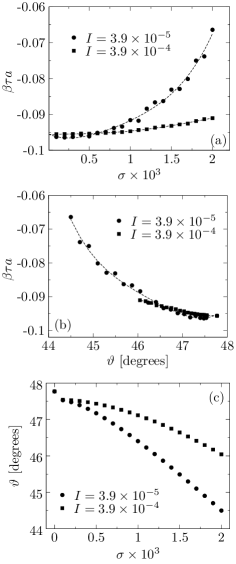
Figure 6: Line tension $\tau$ as a function of the surface charge density $\sigma=\tilde{\sigma}a^{2}/e$ (a) and of the contact angle $\vartheta$ (b) for $T^{*}=0.8T^{*}_{c}$ and $u_{\text{w}}/u=0.69$. The two types of symbols correspond to distinct values of the ionic strength $I=\tilde{I}a^{3}$ in the bulk liquid phase ($\bullet$ for $I=3.9\times 10^{-5}$ ($\tilde{I}=1$mM) and $\scriptstyle\blacksquare$ for $I=3.9\times 10^{-4}$ ($\tilde{I}=10$mM)); the uncertainty of the line tension values corresponds approximately to the size of the symbols. $T^{*}=0.8\times T^{*}_{c}$ is below the wetting transitions, i.e., $T^{*}<T_{w}^{*}(\sigma,I)$, for both ionic strengths $I$ and the whole range of surface charges $\sigma$ shown. The dashed lines are guides to the eye. The rightmost points in panel (a) correspond to the leftmost points in (b). See Appendix A for details concerning the calculation of the line tension. Panel (c) displays the contact angle $\vartheta$ as function of $\sigma$ with $I$ and $T^{*}$ fixed (route (ii)).

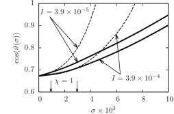
Figure 7: Comparison of $\cos(\vartheta(\sigma))$ for the systems discussed in Fig. 6 (solid lines) with the asymptotic expression given by Eq. (17) (dashed lines) derived in Refs. Kang2 ; Dorr2014 for temperature $T^{*}=0.8T_{c}^{*}$, surface charge density $0\leq\sigma\leq 0.01$ ($0\leq\tilde{\sigma}\leq 1\,\mu\text{C}/\text{cm}^{2}$), and ionic strength $I\in\{3.9\times 10^{-5},3.9\times 10^{-4}\}$ ($\tilde{I}\in\{1\,\text{mM},10\,\text{mM}\}$). The asymptotic expressions apply up to surface charges $\sigma$ for which the dimensionless parameter $\chi=|\sigma|\sqrt{2\pi l_{B}/(\epsilon I)}$ attains unity, which is marked by the vertical arrows.

Figure 6 shows the line tension for the case that the contact angle is varied by using route (ii) for two values of the ionic strength $I$ and for $T^{*}=0.8T^{*}_{c}$. The line tension $\tau(T^{*},\sigma,I)<0$ is a monotonically increasing function of the surface charge density $\sigma>0$, and, as already discussed above in connection with Fig. 5(a), it increases upon decreasing the ionic strength $I$. Here, only small surface charge values ($\sigma=1\times 10^{-4}-2\times 10^{-3}$) have been considered. Accordingly, small contact angles, which correspond to large surface charges, have not been studied. The technical reason for this is that in order to avoid contributions from the corners of the integration box, these corners should be located far away from all interfaces such that the density profiles near the corners attain their bulk values (see Appendix A and Sec. II.3). Achieving this for small contact angles is more difficult in the case of the electrolyte solution than for the pure solvent, mainly due to the density distributions of the ions. Figures 8 and 9 show density distributions of the solvent $\rho_{0}(\bar{x},\bar{z})$ and of the ions $\rho_{\pm}(\bar{x},\bar{z})$ for $\sigma=1\times 10^{-4}$ ($\tilde{\sigma}=0.01\mu$C/cm²) and $\sigma=8\times 10^{-3}$ ($\tilde{\sigma}=0.8\mu$C/cm²), respectively. Both for Fig. 8 and Fig. 9, the bulk densities of the ions are $\rho_{\pm}=I=3.9\times 10^{-5}$ ($\tilde{I}=1$mM). For $\sigma=1\times 10^{-4}$, in Fig. 8 one can see that for the positive ions in the liquid phase the density profile attains its bulk value only in a small portion of the calculation box, which makes it difficult to use the integration box shown in , c.f., Fig. 12 and to carry out the procedure described in Appendix A for the calculation of the line tension. Moreover one can see in, c.f., Fig. 13, which shows examples of the dependence of the estimator $\mathcal{T}(\mathcal{B}^{(1)},\mathcal{B}^{(2)})$ of the line tension (see Appendix A) on the box size for two different surface charge densities, that the amplitude of the variations of the value of $\mathcal{T}(\mathcal{B}^{(1)},\mathcal{B}^{(2)})$, i.e., the uncertainty of the value of the line tension, increases if the surface charge density $\sigma$ increases. Figure 6(a) shows that for small surface charge densities ($\sigma\lesssim 1\times 10^{-3}$) the value of the line tension, the uncertainty of which corresponds approximately to the size of the symbols, is, within the precision of the method described in Appendix A, independent of the ionic strength $I$. However, as the surface charge density increases, the absolute value of the line tension $\tau$ decreases stronger for $I=3.9\times 10^{-5}$ ($\tilde{I}=1$mM) than for $I=3.9\times 10^{-4}$ ($\tilde{I}=10$mM). This is related to the fact that due to screening for $I=3.9\times 10^{-4}$ ($\tilde{I}=10$mM) a larger surface charge is needed to produce the same contact angle as for $I=3.9\times 10^{-5}$ ($\tilde{I}=1$mM) (see Fig. 6(c)). Thus upon increasing $I$, according to route (iii), the contact angle $\vartheta$ increases and so does the strength of the line tension.

Within the approximation of a field-free gas phase the asymptotic behavior

$$\cos(\vartheta(\sigma))\simeq\cos(\vartheta(0))+\frac{\sigma^{2}}{\gamma_{l,g}}\sqrt{\frac{\pi l_{B}}{2\epsilon I}}\left(\frac{\pi}{\vartheta(\sigma)}-1\right)$$ (17)

has been derived in Refs. Kang2 ; Dorr2014 for the case of the dimensionless quantity $\displaystyle\chi:=|\sigma|\sqrt{\frac{2\pi l_{B}}{\epsilon I}}$ being small ($\chi\ll 1$). Figure 7 compares the curves $\cos(\vartheta(\sigma))$ for the systems discussed in Fig. 6 (solid lines) with the corresponding asymptotic form Eq. (17) (dashed lines). The asymptotic expressions are reliable up to surface charge densities $\sigma$ for which $\chi\approx 1$, marked by the vertical arrows in Fig. 7. Hence Eq. (17) applies to small surface charge densities not only in the case of the electric field being confined to a wedge-shaped liquid phase, as in Refs. Kang2 ; Dorr2014 , but also in the case of a non-vanishing electric field in the gas phase.

III.3 Density distributions close to the three-phase contact line

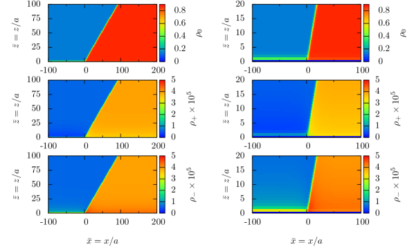
Figure 8: Density distributions of the solvent $\left[\rho_{0}(\bar{x},\bar{z})\right]$, the cations $\left[\rho_{+}(\bar{x},\bar{z})\right]$, and the anions $\left[\rho_{-}(\bar{x},\bar{z})\right]$ for $\sigma=1\times 10^{-4}$ ($\tilde{\sigma}=0.01\mu$C/cm²). The bulk values of the density distribution of the cations and the anions are $\rho_{\pm}=I=3.9\times 10^{-5}$ ($\tilde{I}=1$mM); $\rho_{g}=0.14$ and $\rho_{l}=0.86$ are the bulk values for the gas and the liquid, respectively. The contact angle is $\vartheta\approx 47.5^{\circ}$. The substrate is positively charged. Therefore there is a high (low) density of negative (positive) ions in its vicinity. The panels on the right show close-ups of the plots on the left in the vicinity of the TPCL.

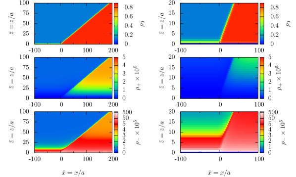
Figure 9: Same as Fig. 8 for $\sigma=8\times 10^{-3}$ ($\tilde{\sigma}=0.8\mu$C/cm²). The contact angle is $\vartheta\approx 28.3^{\circ}$. Note that in this case the density distribution $\rho_{+}$ of the cations in the liquid phase needs more space in order to attain its bulk value $I=3.9\times 10^{-5}$($\tilde{I}=1$mM) than for $\sigma=1\times 10^{-4}$ ($\tilde{\sigma}=0.01\mu$C/cm²) (see Fig. 8).

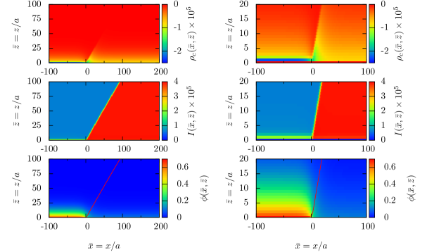
Figure 10: Charge density $\rho_{c}(\bar{x},\bar{z})=\rho_{+}(\bar{x},\bar{z})-\rho_{-}(\bar{x},\bar{z})$, local ionic strength $I(\bar{x},\bar{z})=\tfrac{1}{2}\left(\rho_{+}(\bar{x},\bar{z})+\rho_{-}(\bar{x},\bar{z})\right)$, and electrostatic potential $\phi(\bar{x},\bar{z})=\beta e\tilde{\phi}(\bar{x},\bar{z})$ for $\sigma=1\times 10^{-4}$ ($\tilde{\sigma}=0.01\mu$C/cm²). The contact angle is $\vartheta\approx 47.5^{\circ}$. The red line in the bottom panels for the electrostatic potential indicates the shape $\ell(\bar{x})$ of the liquid-gas interface obtained from Eq. (16). The panels on the right show close-ups of the plots on the left in the vicinity of the TPCL.

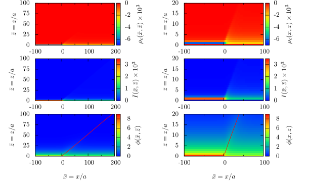
Figure 11: Same as Fig. 10 for $\sigma=8\times 10^{-3}$ ($\tilde{\sigma}=0.8\mu$C/cm²). The contact angle is $\vartheta\approx 28.3^{\circ}$.

The microscopic structure of the electrolyte solution close to the TPCL is illustrated via density maps in Figs. 8 and 9 for $I=3.9\times 10^{-5}$ ($\tilde{I}=1$mM), $T^{*}=0.8T^{*}_{c}$, and two values of the surface charge density: $\sigma=1\times 10^{-4}$($\tilde{\sigma}=0.01\mu$C/cm²) (see Fig. 8) and $\sigma=8\times 10^{-3}$ ($\tilde{\sigma}=0.8\mu$C/cm²) (see Fig. 9) . The contact angles are $\vartheta\approx 47.5^{\circ}$ for $\sigma=1\times 10^{-4}$ and $\vartheta\approx 28.3^{\circ}$ for $\sigma=8\times 10^{-3}$. Apart from the difference in contact angle and from the different densities of anions and cations in the vicinity of the wall due to the difference in surface charge density $\sigma$, one can infer that for larger values of the surface charge the density distributions of the ions differ significantly from their bulk values over larger distances from the substrate. The anion densities $\rho_{-}(z)$ close to the gas-wall interface in Fig. 9 are large because in the present study (see Sec. II.1) we assume a laterally uniform surface charge density, which is not modified by charge regulation. For setups with surface charge densities being determined by charge regulation, significantly smaller surface charge densities would occur and hence smaller ion densities $\rho_{\pm}(z)$ close to the gas-wall interface.

Figures 10 and 11 show the charge density $\rho_{c}(\bar{x},\bar{z})=\rho_{+}((\bar{x},\bar{z})-\rho_{-}(\bar{x},\bar{z})$, the local ionic strength $I(\bar{x},\bar{z})=\tfrac{1}{2}\left(\rho_{+}((\bar{x},\bar{z})+\rho_{-}((\bar{x},\bar{z}))\right)$, and the electrostatic potential $\phi(\bar{x},\bar{z})=\beta e\tilde{\phi}(\bar{x},\bar{z})$ for the same set of parameters as in Figs. 8 and 9, respectively. For a small surface charge density $\sigma$ (see Fig. 10) the charge density $\rho_{c}(\bar{x},\bar{z})$ has a region in the gas close to the liquid-gas interface where $\rho_{c}(\bar{x},\bar{z})$ is less negative than $\rho_{c}(-\infty,\bar{z})$. If one takes a path parallel to the surface at small $\bar{z}$ from the gas side, the charge density $\rho_{c}(\bar{x},\bar{z})$ is quasi constant in the gas phase far away from the liquid-gas interface, increases upon approaching the liquid-gas interface from the gas side, drops to a rather low value on the liquid side of the liquid-gas interface, and ultimately increases towards a constant value in the liquid phase. This charge separation in the vicinity of the liquid-gas interface and of the TPCL is caused by the variation of the local permittivity of the solvent $\varepsilon(\rho_{0}(\bar{x},\bar{z}))$ which is higher in the liquid phase (see Eq. 11). On the other hand, the structure of the local ionic strength distribution $I(\bar{x},\bar{z})$, which for constant $\bar{z}$ interpolates from the value in the gas phase to the value in the liquid phase, is almost independent of $\bar{z}$ within each phase. The electrostatic potential $\phi(\bar{x},\bar{z})$, which is related to the charge density through Poisson’s equation (Eq. (14)), does not follow the liquid-gas interface in that the equipotential lines bend away from it. Moreover, there is an electrostatic potential difference between the liquid and the gas phase in the vicinity of the TPCL. For a large surface charge density $\sigma$ (see Fig. 11), the high charge density $\rho_{c}$ in the vicinity of the substrate on the gas side screens the surface charge of the substrate within a few layers. This is in contrast to the case of small surface charge for which the charge density $\rho_{c}(\bar{x},\bar{z})$ approaches its vanishing bulk value more slowly (compare Fig. 10). This different behavior is due to the nonlinear character of Poisson’s equation (see Eq. (14)); for small values of the surface charge density $\sigma$ its solution is close to the solution of the linearized equation in which the number densities of the ions decay exponentially to their bulk values on the scale of the Debye length $\kappa$ of the bulk phase. In contrast, for large surface charge density $\sigma$ both the density distributions of the ions and the electrostatic potential $\phi$ deviate significantly from the linear solution in the vicinity of the substrate, and the exponential decay is only valid far away from it. For this large value of $\sigma$, the aforementioned nonmonotonic variation of $\rho_{c}(\bar{x},\bar{z})$ in the vicinity of the liquid-gas interface from the gas side is not observed. However, $\rho_{c}(\bar{x},\bar{z})$ becomes more negative in the vicinity of the liquid-gas interface from the liquid side. This qualitative difference as a function of $\sigma$ in the behavior of the charge density in the vicinity of the TPCL results in a different behavior of the electrostatic potential. For large $\sigma$ the difference of the values of the electrostatic potential in the liquid and in the gas phase is not as pronounced as for smaller surface charge densities (see Fig. 10). For all $\sigma$, far away from the substrate the charge density $\rho_{c}(\bar{x},\bar{z})$ and the electrostatic potential $\phi(\bar{x},\bar{z})$ vanish and the local ionic strength attains its bulk value, here $I=3.9\times 10^{-5}$.

IV Conclusions and summary

We have investigated the line tension and the structure of the three-phase contact line (Fig. 1) of an electrolyte solution in contact with a charged substrate by using density functional theory applied to a lattice model Ibagon . For the pure, i.e., salt-free solvent, the equilibrium shape of the liquid-gas interface approaches its asymptotes from above, as expected for systems exhibiting second-order wetting transitions (Fig. 2). Near the wetting transition the line tension vanishes proportional to the contact angle (Fig. 3) which itself goes to zero at the wetting transition temperature. For the electrolyte solution, the equilibrium shape of the liquid-gas interface approaches its asymptote from below as expected for systems exhibiting first-order wetting transitions (Fig. 4). If the contact angle is changed by varying the temperature while keeping the surface charge fixed, the line tension becomes less negative as the temperature is increased (Fig. 5(a)), i.e., as the contact angle is decreased. For fixed temperature, the line tension is more negative for the larger ionic strength (Fig. 5(a)). If the contact angle is changed by varying the surface charge density at fixed temperature, the line tension becomes less negative as the surface charge is increased (Fig. 6(a)). For small surface charges this decrease of the strength of the line tension depends only weakly on the ionic strength (Fig. 6(a)). However, for larger surface charges the decrease of the strength of the line tension is steeper for the smaller ionic strength (Fig. 6(a)). We have also calculated the intrinsic equilibrium structure of the three-phase contact line for various charge densities. For large surface charge densities, nonlinear effects of the Poisson-Boltzmann theory dominate. This results in distributions of the ions and of the electrostatic potential which differ from those for small surface charge densities (Figs. 8, 9, 10, and 11).

On the one hand, technically the lattice model facilitates the reliable determination of these structures and properties. On the other hand, using a lattice model causes a difficulty for calculating the line tension, because within this model the liquid-gas surface tension depends on the orientation of the interfacial plane relative to the underlying lattice. Accordingly, this aspect of our study should be regarded as a first step towards the microscopic calculation of line tensions in electrolyte solutions and should be compared with not yet available results from continuum models for electrolytes. Moreover, for technical reasons the asymptotic behavior of the line tension upon approaching the wetting transition and the influence of a large surface charge densities of the substrate on the line tension could not be addressed within the present approach; they deserve to be analyzed in the future within continuum models.

Appendix A Line tension calculation within the lattice model

For the line tension calculation, computational boxes $\mathcal{B}$ have been used which cut perpendicularly through all interfaces and which are bounded by the substrate-fluid interfaces being located at $z=0$ (Fig. 12(a)). As discussed in Ref. SND , this type of boxes ensures that, for sufficiently large $\mathcal{B}$ and within continuum models, no artificial contributions to the grand canonical free energy $\Omega(\mathcal{B})$ appear, which are due to the edges of $\mathcal{B}$ or due to inhomogeneities caused by the boundaries of $\mathcal{B}$. According to Eq. (15), the grand canonical free energy $\Omega(\mathcal{B})$ of $\mathcal{B}$ per length $L$ of the straight three-phase contact line $T$ (see Fig. 12) is given by

$$\frac{\Omega(\mathcal{B})}{L}=\ \Omega_{b}A(\mathcal{B})+\gamma_{l,g}(\mathcal{B})L_{l,g}(\mathcal{B})+\gamma_{s,l}L_{s,l}(\mathcal{B})$$

$$+\gamma_{s,g}L_{s,g}(\mathcal{B})+\tau,$$ (18)

where $\Omega_{b}=\Omega_{g}=\Omega_{l}=-p$ is the density of the bulk grand potential, i.e., the negative pressure, given by Eq. (3) evaluated at the equilibrium densities, $A(\mathcal{B})$ is the cross-sectional area of $\mathcal{B}$, such that $V(\mathcal{B})=A(\mathcal{B})L$ is the volume of the fluid inside $\mathcal{B}$, $L_{l,g}(\mathcal{B})=z_{P}(\mathcal{B})/\sin(\vartheta)$ is the length of the intersection of the liquid-gas interface inside $\mathcal{B}$ with the $x$-$z$-plane (see the thick magenta line $TP$ in Fig. 12), and $L_{s,l}(\mathcal{B})$ and $L_{s,g}(\mathcal{B})$ are the linear extensions of the substrate-liquid and the substrate-gas interface in the $x$-direction, respectively. The substrate-liquid surface tension $\gamma_{s,l}$ and the substrate-gas surface tension $\gamma_{s,g}$ in Eq. (18) do not depend on $\mathcal{B}$ and they can be inferred from the substrate being in contact with the bulk liquid and bulk gas, respectively. Note that the quantities $A(\mathcal{B})$, $\gamma_{s,l}$, $L_{s,l}(\mathcal{B})$, $\gamma_{s,g}$, and $L_{s,g}(\mathcal{B})$ depend on the choice of the convention for the substrate-fluid interface position (here $z=0$, see Fig. 12(a)), so that the line tension $\tau$ in Eq. (18) depends on this choice of the convention, too.

A difference between continuum and lattice models arises with respect to $\gamma_{l,g}(\mathcal{B})$ in Eq. (18): Within continuum models, $\gamma_{l,g}(\mathcal{B})=\gamma_{l,g}^{(0)}$ is independent of $\mathcal{B}$ and it coincides with the liquid-gas interfacial tension $\gamma_{l,g}^{(0)}$, whereas within lattice models $\gamma_{l,g}(\mathcal{B})$ varies with $\mathcal{B}$ since the tilted free liquid-gas free interface (see the thick magenta line $TP$ in Fig. 12), which is inclined by the contact angle $\vartheta$ with respect to the substrate, in general does not match the underlying lattice grid.

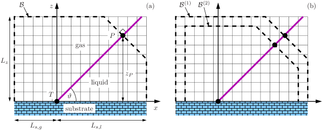
Figure 12: (a) Underlying geometry for calculations of the line tension. The Euler-Lagrange equations in Eq. (12) are solved via an iterative algorithm in a rectangular box which includes as a subset the computational box $\mathcal{B}$ (dashed lines) which is used to determine the line tension. $\mathcal{B}$ encloses the three-phase contact line $T$ and its boundaries cut perpendicularly through all interfaces. It is characterized by the lengths $L_{s,g}$ and $L_{s,l}$ of the substrate-gas and the substrate-liquid interface at the plane $z=0$, respectively, by the width $L_{z}$ in $z$-direction, and by the $z$-coordinate $z_{P}$ of the point $P$, where $\mathcal{B}$ intersects the liquid-gas interface (thick inclined magenta line, forming the contact angle $\vartheta$ with the substrate surface). The convention of the substrate-fluid interfaces being located at $z=0$ affects not only the geometrical quantities $L_{s,g}$, $L_{s,l}$, and $A(\mathcal{B})$, but also the definition of the substrate-gas and the substrate-liquid surface tensions $\gamma_{s,g}$ and $\gamma_{s,l}$, respectively. The system is translationally invariant in the $y$-direction. Note that the boundary cutting through the liquid-gas interface crosses some of the cells, leaving only a fraction of each of them inside $\mathcal{B}$; it is this fraction with which these cells contribute to the total grand canonical free energy. (b) The line tension is determined via the estimator $\overline{\mathcal{T}}(\mathcal{B}^{(1)},\mathcal{B}^{(2)})$ in Eq. (22), which takes two different calculational boxes $\mathcal{B}^{(1)}$ and $\mathcal{B}^{(2)}$ as its arguments (see also Fig. 13).

In order to estimate the line tension $\tau$ in Eq. (18), the contribution $\gamma_{l,g}(\mathcal{B})L_{l,g}(\mathcal{B})$ in Eq. (18) is written in the form

$$\gamma_{l,g}(\mathcal{B})L_{l,g}(\mathcal{B})=\frac{\gamma_{l,g}^{(0)}z_{P}(\mathcal{B})}{\sin(\vartheta)}+\delta_{l,g}(\mathcal{B})$$ (19)

with $\vartheta$ independent of $\mathcal{B}$. Being maximally ignorant of the relative position of the liquid-gas interface with respect to the lattice grid, the probabilities of finding positive or negative deviations $\delta_{l,g}(\mathcal{B})$ are equal such that the expectation value $\langle\delta_{l,g}(\mathcal{B})\rangle$ vanishes. Consequently, according to Eq. (18), the quantity

$$\mathcal{T}(\mathcal{B}):=\ \frac{\Omega(\mathcal{B})}{L}-\Omega_{b}A(\mathcal{B})-\frac{\gamma_{l,g}^{(0)}z_{P}(\mathcal{B})}{\sin(\vartheta)}$$

$$-\gamma_{s,l}L_{s,l}(\mathcal{B})-\gamma_{s,g}L_{s,g}(\mathcal{B})$$ (20)

is expected to vary, within the set of computational boxes $\mathcal{B}$ of the type specified above, as a function of $\mathcal{B}$ around the line tension $\tau$ according to

$$\mathcal{T}(\mathcal{B})=\tau+\delta_{l,g}(\mathcal{B}).$$ (21)

In principle, Eq. (21) facilitates to determine the line tension $\tau$ as the $\mathcal{B}$-independent “background” contribution to $\mathcal{T}(\mathcal{B})$. However, $\mathcal{T}(\mathcal{B})$ depends sensitively on the value $\vartheta$ of the contact angle, which turns out to be difficult to track with the necessary numerical precision. A possible approach to determine the line tension $\tau$ without precise knowledge of the contact angle $\vartheta$ consists of the following: Consider two computational boxes $\mathcal{B}^{(1)}$ and $\mathcal{B}^{(2)}$ with $z_{P}(\mathcal{B}^{(1)})=:z_{1}$ and $z_{P}(\mathcal{B}^{(2)})=:z_{2}$. The contributions $\sim 1/\sin(\vartheta)$ from Eq. (20) cancel in the combination $z_{1}\mathcal{T}(\mathcal{B}^{(2)})-z_{2}\mathcal{T}(\mathcal{B}^{(1)})$ so that instead of Eq. (21) one can use the expression

$$\overline{\mathcal{T}}(\mathcal{B}^{(1)},\mathcal{B}^{(2)}):= \ \frac{z_{1}\mathcal{T}(\mathcal{B}^{(2)})-z_{2}\mathcal{T}(\mathcal{B}^{(1)})}{z_{1}-z_{2}}$$

$$= \ \tau+\frac{z_{1}\delta_{l,g}(\mathcal{B}^{(2)})-z_{2}\delta_{l,g}(\mathcal{B}^{(1)})}{z_{1}-z_{2}}$$ (22)

in order to infer the line tension $\tau$ as that contribution to $\overline{\mathcal{T}}(\mathcal{B}^{(1)},\mathcal{B}^{(2)})$, which is independent of $\mathcal{B}^{(1)}$ and $\mathcal{B}^{(2)}$.

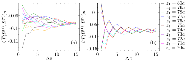
Figure 13: Data for $\overline{\mathcal{T}}(\mathcal{B}^{(1)},\mathcal{B}^{(2)})$ introduced in Eq. (22) for an electrolyte solution with $I=3.9\times 10^{-5}$ ($\tilde{I}=1mM$) at $T^{*}=0.8\times T^{*}_{c}$ for $\sigma=5\times 10^{-4}$ ($\tilde{\sigma}=0.05\mu$C/cm²) (a) and $\sigma=1.8\times 10^{-3}$ ($\tilde{\sigma}=0.18\mu$C/cm²) (b). The various colors correspond to different computational boxes $\mathcal{B}^{(1)}$ in Eq. (22), i.e., they correspond to different distances $z_{1}=z_{P}(\mathcal{B}^{(1)})$ of the point $P$, where the boundary of the box intersects the liquid-gas interface, from the substrate (see Fig. 12(a)). The expression $\overline{\mathcal{T}}(\mathcal{B}^{(1)},\mathcal{B}^{(2)})$ is shown as a function of $\Delta\bar{z}=\bar{z}_{1}-\bar{z}_{2}$ with $z_{2}=z_{P}(\mathcal{B}^{(2)})$ (see Fig. 12(b)). The line tension $\tau$ is inferred from these plots as that contribution to $\overline{\mathcal{T}}(\mathcal{B}^{(1)},\mathcal{B}^{(2)})$, which is constant, i.e., independent of $z_{1}$ and $\Delta z$ (see Eq. (22)).

We have calculated the expression $\overline{\mathcal{T}}(\mathcal{B}^{(1)},\mathcal{B}^{(2)})$ in Eq. (22) by fixing the intersection of box $\mathcal{B}^{(1)}$ with the liquid-gas interface at wall distances $z_{1}\in[30a,40a]$ for the pure solvent and at wall distances $z_{1}\in[70a,80a]$ for the electrolyte solution. The size of box $\mathcal{B}^{(2)}$ has been varied accordingly such that $\Delta z:=z_{1}-z_{2}\in\{a,2a,\cdots,15a\}$. This procedure has been repeated for all integers $z_{1}$ in the corresponding intervals for the pure solvent and for the electrolyte solution. The values of $L_{s,l}$ and $L_{s,g}$ (see Fig. 12) are determined via the position at which the asymptote of the gas-liquid interface intersects the plane $z=0$. The size of the rectangular box used to determine the equilibrium profiles depends on the contact angle $\vartheta$, i.e., for smaller contact angles a larger extension in the $x$-direction is needed. For the pure solvent, as the smaller size we have used $L_{x}\times L_{y}=300a\times 60a$, while as the bigger size $1500a\times 60a$ has been used. For the electrolyte solution a fixed box size of $400a\times 100a$ was used. Figure 13 shows the values of $\overline{\mathcal{T}}(\mathcal{B}^{(1)},\mathcal{B}^{(2)})$ calculated for an electrolyte solution with $I=3.9\times 10^{-5}$ ($\tilde{I}=1mM$), $T^{*}=0.8T^{*}_{c},u_{w}/u=0.69$, and for two values of the surface charge density: $\sigma=5\times 10^{-4}$ ($\tilde{\sigma}=0.05\mu$C/cm²) (Fig. 13(a)) and $\sigma=1.8\times 10^{-3}$ ($\tilde{\sigma}=0.18\mu$C/cm²) (Fig. 13(b)). The variation of $\overline{\mathcal{T}}(\mathcal{B}^{(1)},\mathcal{B}^{(2)})$ with the size of both integration boxes, $\mathcal{B}^{(1)}$ and $\mathcal{B}^{(2)}$, is clearly visible. Nonetheless $\overline{\mathcal{T}}(\mathcal{B}^{(1)},\mathcal{B}^{(2)})$ is distributed around a specific value $\tau$. In order to determine this value $\tau$, which here is called the line tension, that value of $\Delta z$ is chosen which renders the smallest variation in $\overline{\mathcal{T}}(\mathcal{B}^{(1)},\mathcal{B}^{(2)})$ for different $z_{1}$; $\tau$ is taken to be the mean value of the smallest and the largest values of $\overline{\mathcal{T}}(\mathcal{B}^{(1)},\mathcal{B}^{(2)})$ for that particular choice $\Delta z$. We note that the amplitude of the variations in $\overline{\mathcal{T}}(\mathcal{B}^{(1)},\mathcal{B}^{(2)})$ increase with increasing $\sigma$, i.e., with decreasing contact angle $\vartheta$. This can be inferred from the different scales on axes of ordinates in Figs. 13(a) and (b). The corresponding behavior is similar for the other values of the surface charge density considered here. If the surface charge density is fixed and the contact angle $\vartheta$ is varied by changing the temperature, the amplitudes of the variations in $\overline{\mathcal{T}}(\mathcal{B}^{(1)},\mathcal{B}^{(2)})$ increase upon increasing the temperature $T^{*}$, i.e., upon decreasing the contact angle $\vartheta$.

References

- (1) A. Dussaud and M. Vignes-Adler, Langmuir 13, 581 (1997).
- (2) T. Getta and S. Dietrich, Phys. Rev. E 57, 655 (1998).
- (3) W. Qu and D. Li, Colloids and Surfaces A 156, 123 (1999).
- (4) H. Dobbs, Langmuir 15, 2586 (1999).
- (5) T. Pompe and S. Herminghaus, Phys. Rev. Lett 85, 1930 (2000).
- (6) F. Mugele, T. Becker, R. Nikopoulos, M. Kohonen, and S. Herminghaus, J. Adhes. Sci. Technol. 16, 951 (2002).
- (7) Y. Takata, H. Matsubara, Y. Kikuchi, N. Ikeda, T. Matsuda, T. Takiue, and M. Aratono, Langmuir 21, 8594 (2005).
- (8) Y. Djikaev, J. Chem. Phys. 123, 184704 (2005).
- (9) M. Schneemilch and N. Quirke, J. Chem. Phys. 127, 114701 (2007).
- (10) P. G. de Gennes, Rev. Mod. Phys. 57, 827 (1985).
- (11) H. Fan, J. Phys.: Condens. Matter 18 4481 (2006).
- (12) V. Raspal, K. O. Awitor, C. Massard, E. Feschet-Chassot, R. S. P. Bokalawela, and M. B. Johnson, Langmuir 28, 11064 (2012).
- (13) R. Aveyard, J. H. Clint, and T. S. Horozova, Phys. Chem. Chem. Phys. 5, 2398 (2003).
- (14) J. H. Weijs, A. Marchand, B. Andreotti, D. Lohse, and J. H. Snoeijer, Phys. Fluids 23, 022001 (2011).
- (15) J. O. Indekeu, Physica A 183, 439 (1992).
- (16) J. O. Indekeu, Int. J. Mod. Phys. B 8, 309 (1994).
- (17) A. I. Rusanov, Surf. Sci. Rep. 58, 111 (2005).
- (18) L. Schimmele, M. Napiórkowski, and S. Dietrich, J. Chem. Phys. 127, 164715 (2007).
- (19) D. Platikanov, M. Nedyalkov, and A. Scheludko, J. Colloid Interface Sci. 75, 612 (1980).
- (20) J. F. Rodrigues, B. Saramago, M. A. Fortesa, J. Colloid Interface Sci. 239, 577 (2001).
- (21) A. Scheludko, B. V. Toshev, and D. T. Bojadiev, J. Chem. Soc. Faraday Trans. 1 72, 2815 (1976).
- (22) R. Aveyard and J. H. Clint, J. Chem. Soc. Faraday Trans. 91, 2681 (1995).
- (23) G. E. Yakubov, O. I. Vinogradova, and H. J. Butt, Colloid J. 63, 518 (2001).
- (24) R. Aveyard, J. H. Clint, D. Nees, and V. Paunov, Colloids Surf. A 146, 95 (1999).
- (25) J. S. Rowlinson and B. Widom, Molecular Theory of Capillarity (Clarendon, Oxford, 1982).
- (26) B. Widom, J. Phys. Chem. 99, 2803 (1995).
- (27) A. Marmur, J. Colloid Interface Sci. 186, 462 (1997).
- (28) P. Tarazona and G. Navascués, J. Chem. Phys. 75, 3114 (1981).
- (29) C. Bauer and S. Dietrich, Eur. Phys. J. B 10, 767 (1999).
- (30) J. H. Weijs, A. Marchand, B. Andreotti, D. Lohse, and J. H. Snoeijer, Phys. Fluids 23, 022001 (2011).
- (31) M. Zeng, J. Mi, and C. Zhong, Phys. Chem. Chem. Phys. 13, 3932 (2011).
- (32) F. Bresme and N. Quirke, Phys. Rev. Lett. 80, 3791 (1998).
- (33) F. Bresme and N. Quirke, Phys. Chem. Chem. Phys. 1, 2149 (1999).
- (34) T. Werder, J. H. Walther, R. L. Jaffe, T. Halicioglu, and P. Koumoutsakos, J. Phys. Chem. B 107, 1345 (2003).
- (35) J. T. Hirvi and T. A. Pakkanen, J. Chem. Phys. 125, 144712 (2006).
- (36) R. C. Dutta, S. Khan, and J. K. Singh, Fluid Phase Equil. 302, 310 (2011) [Corrigendum: Fluid Phase Equil. 334, 205 (2012)].
- (37) R. Ramírez, J. K. Singh, F. Müller-Plathe, and M. C. Böhm, J. Chem. Phys. 141, 204701 (2014).
- (38) M. Kulmala, H. Vehkamäki, A. Lauri, E. Zapadinsky, A. I. Hienola, in Nucleation and Atmospheric Aerosols, edited by C. D. O’Dowd and P. E. Wagner (Springer Netherlands, Dordrecht, 2007) p. 302.
- (39) B. J. Block, S. Kim, P. Virnau, and K. Binder, Phys. Rev. E 90, 062106 (2014).
- (40) M. Bier and L. Harnau, Z. Phys. Chem. 226, 807 (2012).
- (41) I. Ibagon, M. Bier, and S. Dietrich, J. Chem. Phys. 138, 214703 (2013).
- (42) I. Ibagon, M. Bier, and S. Dietrich, J. Chem. Phys. 140, 174713 (2014).
- (43) R. Digilov, Langmuir 16, 6719 (2000).
- (44) T. Chou, Phys. Rev. Lett. 87, 106101 (2001).
- (45) J. Buehrle, S. Herminghaus, and F. Mugele, Phys. Rev. Lett. 91, 086101 (2003).
- (46) K. H. Kang, I. S. Kang, and C. M. Lee, Langmuir 19, 6881 (2003).
- (47) K. H. Kang, I. S. Kang, and C. M. Lee, Langmuir 19, 9334 (2003).
- (48) A. Dörr and S. Hardt, Phys. Fluids 26, 082105 (2014).
- (49) C. Quilliet and B. Berge, Curr. Opin. Colloid Interface Sci. 6, 34 (2001).
- (50) A. Dörr and S. Hardt, Phys. Rev. E 86, 022601 (2012).
- (51) S. Das and S. K. Mitra, Phys. Rev. E 88, 033021 (2013).
- (52) B. Berge, C. R. Acad. Sci. II 317, 157 (1993).
- (53) F. Mugele and J.-C. Baret, J. Phys.: Condens. Matter 17, R705 (2005).
- (54) J. D. Jackson, Classical Electrodynamics, 3rd ed., (Wiley, New York, 1999).
- (55) D. J. Tobias, A. C. Stern, M. D. Baer, Y. Levin, and C. J. Mundy, Annu. Rev. Phys. Chem. 64, 339 (2013).
- (56) M. Born, Z. Phys. 1, 45 (1920).
- (57) R. Pandit, Phys. Rev. B 26, 5112 (1982).
- (58) R. Pandit and M. Wortis, Phys. Rev. B 25, 3226 (1982).
- (59) D. Bonn, J. Eggers, J. Indekeu, J. Meunier, and E. Rolley, Rev. Mod. Phys. 81, 739 (2009).
- (60) R.-J. Merath, Microscopic calculation of line tensions, doctoral thesis, Universität Stuttgart (2008).