11email: gonzalo@ifsc.usp.br
A complex network approach to cloud computing
Abstract
Cloud computing has become an important means to speed up computing. One problem influencing heavily the performance of such systems is the choice of nodes as servers responsible for executing the users’ tasks. In this article we report how complex networks can be used to model such a problem. More specifically, we investigate the performance of the processing respectively to cloud systems underlain by Erdős-Rényi and Barabási-Albert topology containing two servers. Cloud networks involving two communities not necessarily of the same size are also considered in our analysis. The performance of each configuration is quantified in terms of two indices: the cost of communication between the user and the nearest server, and the balance of the distribution of tasks between the two servers. Regarding the latter index, the ER topology provides better performance than the BA case for smaller average degrees and opposite behavior for larger average degrees. With respect to the cost, smaller values are found in the BA topology irrespective of the average degree. In addition, we also verified that it is easier to find good servers in the ER than in BA. Surprisingly, balance and cost are not too much affected by the presence of communities. However, for a well-defined community network, we found that it is important to assign each server to a different community so as to achieve better performance.
pacs:
89.75.FbStructures and organization in complex systems and 89.20.FfComputer science and technology and 89.20.HhWorld Wide Web, Internet1 Introduction
With the booming of the Internet, an impressive mass of computing resources, encompassing both machine and data, became broadly available. At the same time, the number of users grew largely, implying in a growing demand to Internet collaborative access in a number of machines and platforms. Cloud computing emerged as the natural integration of these two trends. The basic idea in this paradigm is to define integrated, distributed, servers capable of supplying services to users through Internet. In addition, since the data in the cloud system has to be widely accessible in many places and for many users, multiple servers are required. As a consequence of its reliance on the Internet, cloud systems tend to have complex topologies, which compounds the choice of where in the network the servers should be placed. In particular, the distribution of the servers should lead to small communication times between users and servers, without overloading any of the servers.
Complex networks have become an important subject in science and technology because of their ability to represent and model a large number of complex systems such as society, protein interaction, transportation, among many others Barabasi:2002:LIN:829575 ; Newman:2010:NI:1809753 ; costa2007characterization . In computer science, complex networks have been used, for instance, in the study of the topology of the Internet faloutsos99:_inter , the Web baldi03:_model_inter_web , email communications tyler03:_email , the complexity of software systems ma05 , and modeling grid computing˜da2005complex ; de2008effects ; travieso2011effective ; travieso2013predicting ; prieto-castillo14 . In the latter field, complex networks were used to represent task execution in grid computing environments, with the tasks being supplied by a master, on demand from worker processors, which were distributed along the network topology. Contrariwise, in cloud computing several users concur for access to a small number of servers.
In the present work we extend the use of complex networks to modeling and evaluating the performance of multiple-severs cloud computing environments. More specifically, we quantify the effect of different topologies —namely Erdos-Rényi˜Erdos-Renyi:1959 , Barabasi-Albert˜Barabasi97 and a modular model— with respect to the positioning of servers in the network topology. For simplicity’s sake, we consider only pairs of servers in the cloud environments.
The article starts by presenting the basic concepts and methods adopted, and follows by presenting how cloud environments can be represented in complex networks, and investigating the performance of such configurations for different placements of servers in the network topology. We have found that the distribution of servers in cloud computing environments is determinant for the performance, quantified in terms of communication cost and balance. In addition, the best configurations depend strongly on the network topology.
2 Methodology
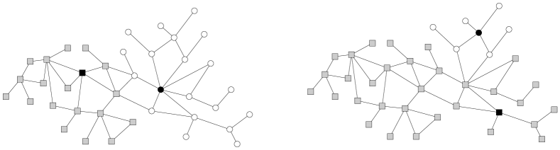
We consider here a network that provides a communication infrastructure for agents placed on its nodes. Some agents (called “servers”) will be chosen to provide services for the other agents (the “clients”). A request for a service is forwarded by a client to the closest server following a shortest path, and the response from the server follows the same path in the reverse order. Once the servers are placed in the network, each client is assigned to the closest server. Thus, for good efficiency on the delivery and execution of the services, the servers must be placed in the network such that they are relatively close to the their clients and each server is responsible for answering requests from about the same number of other clients. Figure 1 shows two contrasting situations regarding the placement of two servers in a same network. On the left part of the figure, a good balance is achieved because each server is associated to similar number of clients. Contrariwise, on the right, one of the servers resulted with only six clients, while a much larger number of clients is associated to the other server.
To quantitatively evaluate the aspects above, given a choice of servers we compute two measurement: the average cost and the balance, defined as follows.
Let be the server associated with client (i.e. the server that is closest to ). The average cost is defined as
| (1) |
where is the shortest path length from node to node in the network. The factor is include to account for the request and response communication costs. The sum runs over all clients .
The balance should quantify if all servers receive work from approximately the same number of clients. Let be the set of clients associated with server , and its cardinality. We define the balance as the ratio from the smaller to the larger of these sets:
| (2) |
where the and run over all servers .
We want to evaluate the effect of network topology on this dynamical process. For simplicity and computational efficiency, we consider the case of only two servers. Given a pair of servers, we choose to which server the clients are associated, using the distance matrix of the network and choosing the nearest server for each client. Afterward the values of average cost and balance are computed for this pair of servers using the expressions above. The process is repeated for all pairs of servers in the network. A good pair of servers should have simultaneously a large value of balance and a small value of average cost. We define the elite of server pairs as the intersection of the pairs within the 20% with best (smallest) values of average cost and the 20% with the best (largest) value of balance. For each evaluated network we compute: the smallest values of average cost and largest value of balance for all pairs, the threshold values of average cost and balance needed to include a pair in the elite, the average values of average cost and balance for all pairs, the average values of average cost and balance for the pairs in the elite, and the number of pairs in the elite.
We consider now the effect of community structure in the network over the balance and average cost. We want to quantify the effects of community separation and differences in community sizes. The network model used consists of nodes, each associated with a given community. We fix the number of communities in two, and associate nodes to the first community and nodes to the second, where and means rounding to the closest integer. Without losing generality, in the following we choose community 1 to be the smallest, and therefore . Each pair of nodes is connected according with the following:
- Inside community 1
-
If both nodes are from community 1, they are connected with probability
(3) where is the desired average degree and the parameter controls the community structure as will be discussed below.
- Inside community 2
-
When both nodes are from community 2, the connection probability is
(4) - Between communities
-
If the nodes are in different communities, the probability of connection is given by
(5)
Different values are chosen for the probability in the two communities to achieve the same average degrees for nodes in both communities. If the same value of probability is used for a small and a large community, each node in the smaller community have less other possible nodes inside the same community to connect, and therefore has a smaller expected degrees than the nodes in the larger community. For the values in Equations (3) to (5), the average degree of nodes in the first community is (for large values of ):
For the second community, the average degree is:
The value is a community strength parameter and quantifies how much of the existing connectivity in the first community is used for connections with the other community. Note that, if , then and there are no connections between the two communities. Therefore values of near zero result in a pronounced community structure. On the other hand, if , we have , and all links from community 1 are to community 2. In this last case, if the two communities are of the same size (), all links from nodes in community 2 go to nodes in community 1, and the network is bipartite. In the general case, links still exist among the nodes in the largest community. A value of corresponds to the case where half of the links in community 1 go to the same community, and half to the other community and is the largest value of interest to us here.
3 Results and discussion
3.1 ER and BA networks
Figure 2 shows the result of this evaluation for the Erdős-Rényi (ER) and Barabási-Albert (BA) network models with varying values of average degree. We used these models to evaluate the effect of degree heterogeneity. Each network has nodes and we generate networks for each model/parameter combination to compute average and standard deviation of each measurement.
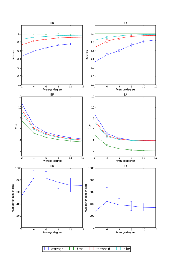
First we notice that the theoretical maximum value of balance is achieved for some node pair in most networks. Also, with the exception of small values of average degree, the balance achieved by pairs in the elite is close to the maximum in both models. It can be seen also that the values of balance (network and elite averages, as well as threshold) for ER networks are slightly better than for BA networks. This is possibly due to the excessive influence of the hubs in the BA topology, making it more sensitive to the choice of pairs.
The situation is different with regard to communication costs, where BA networks are better (with the exception of network with high average degree). It is interesting to note also that the difference in costs for the best and average pairs is much larger in BA networks. This is due to the fact that in these networks, the hubs are central (in the closeness centrality sense) and therefore have small average distances to the other network nodes. If two hubs are chosen in a pair, the communication costs for the pair will be small. But pairs with two hubs are a small minority of all the possible pairs, and therefore do not significantly affect the averages.
The networks have nodes, and therefore there are about distinct pair. For the elite, we choose the pairs that are in the 20% better in cost and in balance. If the two criteria were unrelated, the expected number of pairs in the elite would be . As can be seen in Figure 2, the number of pairs in the elite of ER networks is close to this expected value, with significant differences only for small average degrees. On the other hand, in BA networks the number of pairs in the elite is much lower, about half of the number in the ER networks. This suggests that in topologies with strong degree heterogeneity the efficiency is much more sensitive to the choice of the pair of servers.
3.2 Communities
Figure 3 shows the impact of changes in community sizes () in the balance and cost, for different values of . As expected, for there is no influence of the division of nodes in communities, as the communities are not well separated. For smaller values of we can see some influence of in the balance, but almost no influence in cost. Differences in the sizes of the communities decrease the values of balance, but affect mostly the average of all pairs, and not the average of the elite pairs.
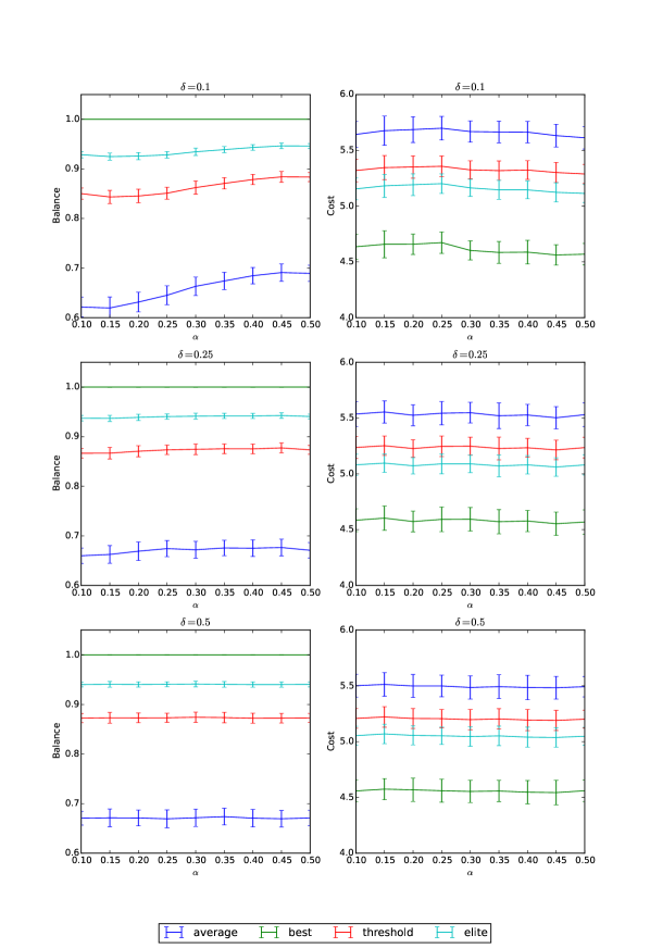
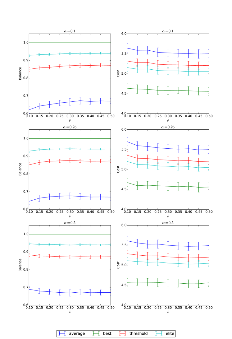
Figure 4 shows the effect of varying (for some values of ). For communities of the same size () there is almost no influence of , with a slightly better balance and worst average cost if is small. For smaller values of (i.e. if there is a larger difference in the sizes of the two communities) a clear trend is seen where smaller values of lead to worse values of balance and cost. This means that a network with communities of different sizes and strong community separation is not well suited for this kind of dynamics.
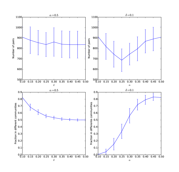
The previous results are complemented by the ones presented in figure 5, where we fix and change (left) or fix and change (right), and evaluate the number of pairs in the elite (top) and the fraction of these elite pairs where each element is in a different community (bottom). On the top left we see that, for communities of the same size, the number of pair in the elite is not affected by the strength of the separation of communities. The bottom left plot shows that for small values of almost all pairs in the elite have nodes in different communities. This means that, under strong community structure, a good efficiency can only be achieved by putting one server in each community. On the top right we see that in the case of a relatively strong community structure (), the number of pairs in the elite decreases as is decreased from to , but increases again afterward. As decreases, the communities are of different sizes, and it becomes more difficult to find pairs of nodes that at the same time are close to the client nodes and equally divide those clients between themselves. The increase below can be explained by looking at the bottom right plot, where we see that fraction of elite pairs with nodes in different communities sharply decreases as decreases. This means that, as one of the communities decreases in size, it becomes advantageous putting both server nodes in the largest community, as the increased cost for the small community is of little total influence.
4 Conclusion
This article has investigated the effect of distinct distribution of servers in cloud computing environments with respect to three network topology, namely ER, BA and modular. In order to better discuss and organize the investigation, we classified as elite the pairs of servers with top performance regarding both communication cost and balance.
Several results have been obtained. First, we have that ER generally provides better balance in detriment of communication cost, while BA provides complementary characteristics. In addition, the elite pairs of servers are more populous in the ER than in the BA networks, and the difference between the best and average pairs is larger in the latter. The investigation of the modular networks was performed while varying the number of nodes in each community and the strength of connection between them. Though the balance is affected by the relative size of the communities, little effect has been observed regarding communication cost. Also, for communities with similar size, the strength of interconnection between communities was not found to influence either communication cost or balance. However, if the communities have different sizes, less interconnection between them worsens both balance and cost. When the separation between the communities is pronounced, most of the elite pairs will have each of its server in different communities. All in all, we have confirmed that the distribution of servers in cloud computing environments can be critical for the performance in terms of communication cost and balance, with the best configurations depending heavily on the network topology.
Future works could address more than a pair of servers, other network topologies, and consider the effect of specific network features on the performance.
Acknowledgements.
OMB is grateful to CNPq (307797/2014-7 and 484312/2013-8). LdFC is grateful to FAPESP (2011/50761-2), CAPES, NAP-PRP-USP, and CNPq (307333/2013-2),References
- [1] A.-L. Barabási. Linked. Perseus Publishing, 1 edition, 2002.
- [2] M. Newman. Networks: An Introduction. Oxford University Press, Inc., New York, NY, USA, 2010.
- [3] L. da Fontoura Costa, F. A. Rodrigues, G. Travieso, and P. R. Villas Boas. Characterization of complex networks: A survey of measurements. Advances in Physics, 56(1):167–242, 2007.
- [4] M. Faloutsos, P. Faloutsos, and C. Faloutsos. On power-law relationships of the Internet topology. Comput. Commun. Rev., 29(4):251–262, 1999.
- [5] P. Baldi, P. Frasconi, and P. Smyth. Modeling the Internet and the Web: Probabilistic Methods and Algorithms. John Wiley & Sons, Chicester, 2003.
- [6] J.R. Tyler, D.M. Wilkinson, and B.A. Huberman. Email as spectroscopy: Automated discovery of community structure within organizations. In M. Huysman, E. Wenger, and V. Wulf, editors, Communities and Technologies, pages 81–96. Springer, New York, 2003.
- [7] Y. Ma, K. He, and D. Du. A qualitative method for measuring the structural complexity of software systems based on complex networks. In APSEC ’05, pages 257–263, 2005.
- [8] L. da Fontoura Costa, G. Travieso, and C. A. Ruggiero. Complex grid computing. The European Physical Journal B-Condensed Matter and Complex Systems, 44(1):119–128, 2005.
- [9] A. F. de Angelis, G. Travieso, C. A. Ruggiero, and L. da Fontoura Costa. On the effects of geographical constraints on task execution in complex networks. International Journal of Modern Physics C, 19(06):847–853, 2008.
- [10] G. Travieso and L. da Fontoura Costa. Effective networks for real-time distributed processing. Journal of Systems Science and Complexity, 24(1):39–50, 2011.
- [11] G. Travieso, C. A. Ruggiero, O. M. Bruno, and L. da Fontoura Costa. Predicting efficiency in master–slave grid computing systems. Journal of Complex Networks, 1(1):63–71, 2013.
- [12] F. Prieto-Castillo, A. Astillero, and M. Botón-Fernandéz. A stochastic process approach to model distributed computing on complex networks. Journal of Grid Computing, pages 1–18, 2014.
- [13] P. Erdős and A. Rényi. On random graphs. Publicationes Mathematicae, 6:290–297, 1959.
- [14] A.-L. Barabási and R. Albert. Emergence of scaling in random networks. Science, 286:509–512, 1997.